Graphical Modelling in Genetics
and Systems Biology

Graphical modelling in its modern form was pioneered by Lauritzen and Wermuth [43] and Pearl [55] in the $1980$s, and has since found applications in fields as diverse as bioinformatics [28], customer satisfaction surveys [37] and weather forecasts [1]. Genetics and systems biology are unique among these fields in the dimension of the data sets they study, which often contain several thousand variables and only a few tens or hundreds of observations. This raises problems in both computational complexity and the statistical significance of the resulting networks, collectively known as the “curse of dimensionality”. Furthermore, the data themselves are difficult to model correctly due to the limited understanding of the underlying phenomena. In the following, we will illustrate how such challenges affect practical graphical modelling and some possible solutions.

1 Background and Notation

Graphical models [39, 55] are a class of statistical models composed by a set $\mathbf{X}=\{X_{1},X_{2},\ldots,X_{p}\}$ of random variables describing the quantities of interest and a graph $\mathcal{G}=(\mathbf{V},E)$ in which each node or vertex $v\in\mathbf{V}$ is associated with one of the random variables in $\mathbf{X}$. The edges $e\in E$ are used to express direct dependence relationships among the variables in $\mathbf{X}$. The set of these relationships is often referred to as the dependence structure of the graph. Different classes of graphs express these relationships with different semantics, which have in common the principle that graphical separation of two vertices implies the conditional independence of the corresponding random variables [55]. Examples most commonly found in literature are Markov networks [72, 21], which use undirected graphs; chain graphs [17], which use partially directed graphs; and Bayesian networks [53, 41], which use directed acyclic graphs.

In principle, there are many possible choices for the joint distribution of $\mathbf{X}$, depending on the nature of the data and the aims of the analysis. However, literature has focused mostly on two cases: the discrete case [72, 33], in which both $\mathbf{X}$ and the $X_{i}$ are multinomial random variables, and the continuous case [72, 31], in which $\mathbf{X}$ is multivariate normal and the $X_{i}$ are univariate normal random variables. In the former, the parameters of interest are the conditional probabilities associated with each variable, usually represented as conditional probability tables; in the latter, the parameters of interest are the partial correlation coefficients between each variable and its neighbours in $\mathcal{G}$.

The estimation of the structure of $\mathcal{G}$ is called structure learning [39, 21], and consists in finding the graph that encodes the conditional independencies present in the data. Ideally it should coincide with the dependence structure of $\mathbf{X}$, or it should at least identify a distribution as close as possible to the correct one in the probability space. Several algorithms have been presented in literature for this problem. Despite differences in theoretical backgrounds and terminology, they can all be traced to three approaches: constraint-based (which are based on conditional independence tests), score-based (which are based on goodness-of-fit scores) and hybrid (which combine the previous two approaches). For some examples, see Castelo and Roverato [11], Friedman et al. [30], Larrañaga et al. [42] and Tsamardinos et al. [71]. All these structure learning algorithms operate under a set of common assumptions:

• there must be a one-to-one correspondence between the nodes in the graph and the random variables in $\mathbf{X}$; this means in particular that there must not be multiple nodes which are deterministic functions of a single variable;

• observations must be independent. If some form of temporal or spatial dependence is present, it must be specifically accounted for in the definition of the network, as in dynamic Bayesian networks [39];

• every combination of the possible values of the variables in $\mathbf{X}$ must represent a valid, observable (even if really unlikely) event.

On the other hand, the structure of the network can also be specified from prior knowledge of the phenomenon underlying the data; in this case the graphical model implements an expert system [16, 12]. This is rarely done in practice, especially in genetics and systems biology, because available information are typically scarce or unreliable. It is far more common to use such information to inform the choices made by a structure learning algorithm, thus making the best use of the data [51].

The structure of a graphical model has two important properties. The first is that it defines the decomposition the probability distribution of $\mathbf{X}$, called the global distribution, into a set of local distributions. For practical reasons, each local distribution should involve only a small number of variables when applying graphical modelling to high dimensional problems. For Bayesian networks it is related to the chain rule of probability [41]; it takes the form

$$\operatorname{P}(\mathbf{X})=\prod_{i=1}^{p}\operatorname{P}(X_{i}\mid\Pi_{X_{i}})$$ (1.1)

so that each local distribution is associated with a single node $X_{i}$ and depends only on the joint distribution of its parents $\Pi_{X_{i}}$. This decomposition holds for any Bayesian network, regardless of its graph structure. In Markov networks local distributions are associated with the cliques $\mathbf{C}_{1}$, $\mathbf{C}_{2}$, $\ldots$, $\mathbf{C}_{k}$, the maximal subsets of nodes in which each element is adjacent to all the others:

$$\operatorname{P}(\mathbf{X})=\prod_{i=1}^{k}\psi_{i}(\mathbf{C}_{i}).$$ (1.2)

The functions $\psi_{1},\psi_{2},\ldots,\psi_{k}$ are called Gibbs’ potentials [55], factor potentials [12] or simply potentials, and are non-negative functions representing the relative mass of probability of each clique. They are proper probability or density functions only when the graph is decomposable or triangulated, that is, when it contains no induced cycles other than triangles. In this case the global distribution factorises again according to the chain rule and can be written as

$$\operatorname{P}(\mathbf{X})=\frac{\prod_{i=1}^{k}\operatorname{P}(\mathbf{C}_{i})}{\prod_{i=1}^{k}\operatorname{P}(\mathbf{S}_{i})}$$ (1.3)

where $\mathbf{S}_{i}$ are the nodes of $\mathbf{C}_{i}$ which are also part of any other clique up to $\mathbf{C}_{i-1}$ [55].

The second important property is that the Markov blanket of each node can be easily identified from the structure of the graph. For instance, in Bayesian networks the Markov blanket of a node $X_{i}$ is the set consisting of the parents of $X_{i}$, the children of $X_{i}$ and all the other nodes sharing a child with $X_{i}$ [55]. Since the Markov blanket is defined as the set of nodes that makes the target node (i.e. $X_{i}$) independent from all the other nodes in $\mathbf{X}$, it provides a theoretically-sound solution to the feature selection problem [40].

2 Data and Models in Statistical Genetics and Systems Biology

In genetics and systems biology, graphical models are employed to describe and identify interdependencies among genes and gene products, with the eventual aim to better understand the molecular mechanisms linking them. Data made commonly available for this task by current technologies fall into three groups:

1. gene expression data [28, 65], which measure the intensity of the activity of a particular gene through the presence of messenger RNA (mRNA, for protein-coding genes) or other kinds of non-coding RNA (ncRNA, for non-coding genes);

2. protein signalling data [58], which measure the proteins produced as a result of each gene’s activity;

3. sequence data [50], which provide the nucleotide sequence of each gene. For both biological and computational reasons, such data contain mostly single-nucleotide polymorphisms (SNPs) – genes which vary in only one nucleotide between individuals – having only two possible alleles, called biallelic SNPs.

In the case of gene expression and protein signalling data (Sections 2.1 and 2.2), we are interested in grouping them into tempporal sequences determining some molecular process (the functional pathways). Bayesian networks are naturally suited to this task. If we assign each gene to one node in the network, edges represent the interplay between different genes. They can describe either direct interactions or indirect influences that are mediated by unobserved genes. This is a crucial property because it is impossible in practice to completely observe a complex molecular process: either we do not know all the genes involved or we may be unable to obtain reliable measurements of all their expression levels. Furthermore, under appropriate conditions [56, 39] edge directions may be indicative of the causal relationships in the underlying pathways. In that case, the Bayesian network reflects the ordering of connections between pathway components and the actual flow of the molecular process.

Similar considerations can be made when protein signalling data are used just to identify protein-protein interactions, limiting ourselves to the study of the cell’s physiology.

On the other hand, in sequence data analysis (Section 2.3) we are interested in modelling the behaviour of one or more phenotypic traits (e.g. the presence of a disease in humans, yield in plants, milk production in cows, etc.) by capturing direct and indirect causal genetic effects. Unless some prior knowledge on the genetic architecture of a trait is available, a large set of genes spread over the whole genome is required for such effects to be detectable. If the focus is on identifying the genes that are strongly associated with a trait, the analysis is called a genome-wide association study (GWAS).

Applications of Bayesian networks to sequence data are more problematic than in the previous cases; some care must be taken in their interpretation as causal models. Edges linking genes to a trait can be considered direct associations. As was the case for gene expression data, under appropriate conditions such associations may actually be indicative of real causal effects. On the other hand, edges linking genes to other genes arise from the genetic structure of the individuals in the sample. It is expected, for example, that genes that are located near each other on a chromosome are more likely to be inherited together during meiosis, and are therefore said to be genetically linked [22]. Furthermore, even genes that are far apart in the genome can be in linkage disequilibrium (LD) if some of their configurations occur more often or less often than it would be expected from their marginal frequencies. Both these phenomena induce associations between the genes, but not cause-effects relationships. From a strictly causal point of view, a chain graph in which genes are linked by undirected edges and the only directed edges are the ones incident on the traits provides a better visual representation of the network structure.

2.1 Gene Expression Data

Gene expression data are typically composed of a set of intensities measuring the abundance of several RNA patterns, each meant to probe a particular gene. These intensities are measured either radioactively or fluorescently, using labels that mark the desired RNA patterns [20, 46, 48].

The measured abundances present several limitations. First of all, microarrays measure abundances only in terms of relative probe intensities, not on an absolute scale. As a result, comparing different studies or including them in a meta-analysis is difficult in practice without the use of rank-based methods [8]. Furthermore, even within a single study abundance measurements are systematically biased by batch effects introduced by the instruments and the chemical reactions used in collecting the data [61].

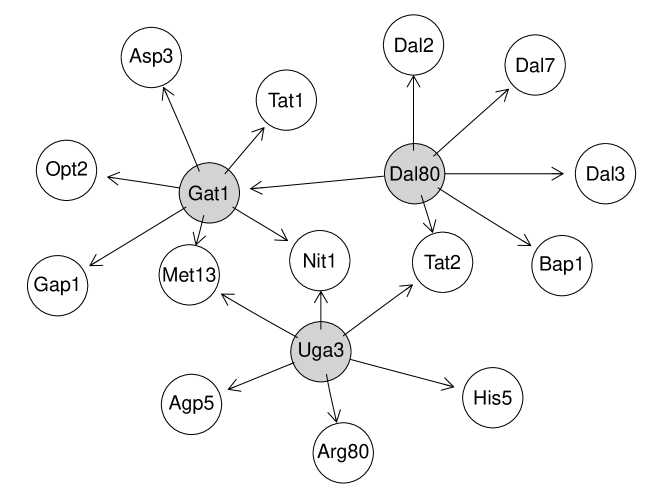
Figure 2.1: A Bayesian network learned from gene expression data and used as an example in Friedman [24]. Grey nodes correspond to the regulators of the network, the genes controlling the expression of the other (target) genes involved in a molecular process.

By their nature, gene expression data are modelled as continuous random variables and are investigated using Pearson’s correlation, either assuming a Gaussian distribution or applying results from robust statistics [34, 69]. The simplest graphical models used for gene expression data are relevance networks [9], also known in statistics as correlation graphs. Relevance networks are constructed by estimating the correlation matrix of the genes and thresholding its elements, so that weak correlations are set to zero. Finally, a graph is drawn in order to depict the remaining strong correlations.

Covariance selection models [19], also known as concentration graphs or graphical Gaussian models [72], consider conditional rather than marginal dependencies; the presence of an edge is determined by the value of the corresponding partial correlation. In the context of systems biology, the resulting graphs are often called gene association networks, and are not trivial to estimate from high-dimensional genomic data. Several solutions have been proposed in literature, based either on James-Stein regularisation [60, 59] or on different penalised maximum likelihood approaches [47, 5, 23].

Both gene relevance and gene association networks are undirected graphs. The application of Bayesian networks to learn large-scale directed graphs from microarray data was pioneered by Friedman et al. [29], and has also been reviewed more recently in Friedman [24] (see Figure 2.1). The high dimensionality of the model, combined with low sample sizes, means that inference procedures are usually unable to identify a single best Bayesian network, settling instead on a set of equally well behaved models. For this reason, it is important to incorporate prior biological knowledge into the network through the use of informative priors [51] and to produce confidence scores in its graphical features [35, 26].

2.2 Protein Signalling Data

Figure 2.2: The Bayesian network learned from the protein-signalling data in Sachs et al. [58] using model averaging and data from several experiments performed under different stimulatory and inhibitory cues.

Protein signalling data are similar to gene expression data in many respects, and in fact are often used to indirectly investigate the expression of a set of genes. In general, the relationships between proteins are indicative of their physical location within the cell and of the development over time of the molecular processes they are involved in.

From a modelling perspective, all the approaches covered in Section 2.1 can be applied to protein signalling data with little or no change. However, it is important to note that protein signalling data sometimes have sample sizes that are much larger than either gene expression or sequence data; an example is the study from Sachs et al. [58] on how to derive a causal Bayesian network from multi-parameter single-cell data (Figure 2.2).

2.3 Sequence Data

Sequence data are fundamentally different from both gene expression and protein signalling data, for several reasons. First, sequence data provide direct access to the genome’s information, without relying on indirect measurements. As a result, they provide a closer view of the genetic layout of an organism than other approaches. Second, sequence information is intrinsic to each individual, and does not vary over time; therefore, the inability of static Bayesian networks to model feedback loops is not a limitation in this case.

Furthermore, sequence data is naturally defined on a discrete rather than continuous domain. Each gene has a finite number of possible states, determined by the number of combinations of nucleotides differing between the individuals in the sample. In the case of biallelic SNPs, each SNP $X_{i}$ differs at a single base-pair location and has only three possible variants. They are determined by the (unordered) combinations of the two nucleotides observed at that location, called the alleles, and are often denoted as “AA”, “Aa”, “aa”. The “A” and “a” labels can be assigned to the nucleotides in several ways; for instance, “A” can be chosen as either the most common in the sample (which makes models easier to interpret) or by following the alphabetical order of the nucleotides (which makes the labelling independent from the sample). “AA” and “aa” individuals are said to be homozygotes, because both nucleotides in the pair have the same allele; “Aa” individuals are said to be heterozygotes.

From a graphical modelling perspective, modelling each SNP as a discrete variable is the most convenient option; multinomial models have received much more attention in literature than Gaussian or mixed ones. On the other hand, the standard approach in genetics is to recode the alleles as numeric variables, e.g.

$$X_{i}=\left\{\begin{aligned} 1&\text{ if the SNP is ``AA''}\\ 0&\text{ if the SNP is ``Aa''}\\ -1&\text{ if the SNP is ``aa''}\end{aligned}\right. X_{i}=\left\{\begin{aligned} 2&\text{ if the SNP is ``AA''}\\ 1&\text{ if the SNP is ``Aa''}\\ 0&\text{ if the SNP is ``aa''}\end{aligned}\right.\,.$$ or (2.1)

In both cases, the recoded variables are typically modelled using an additive Bayesian linear regression model of the form

$$\mathbf{y}=\mu+\sum_{i=1}^{n}X_{i}g_{i}+\boldsymbol{\varepsilon}, g_{i}\sim\pi_{g_{i}},\,\boldsymbol{\varepsilon}\sim N(\mathbf{0},\mathrm{\Sigma})$$ (2.2)

where $g_{i}$ denotes the effect of gene $X_{i}$, $\mathbf{y}$ is the trait under study and $\mu$ is the population mean. The matrix $\mathrm{\Sigma}$ models the relatedness of the subjects, which is called kinship in genetics, and populations structure [4]. In human genetics, it is often assumed to be the identity matrix, which implies the assumptions that individuals are unrelated. Several implementations of Equation 2.2 based on linear mixed models and penalised regressions have been proposed, mostly within the framework of Bayesian statistics. Some examples are the Genomic BLUP (GBLUP), BayesA and BayesB from Meuwissen et al. [49], the Bayesian LASSO from Park and Casella [54] and the BayesC$\pi$ from Habier et al. [18].

Figure 2.3: Different approaches to GWAS. On the top, classic additive Bayesian linear regression models with and without feature selection. On the bottom, more complex models based on Bayesian networks.

Graphical models, and Bayesian networks in particular, provide a systematic way to categorise and extend such models. Consider the four different models shown in Figure 2.3. The classic additive model from Equation 2.2 is shown in the top-left panel; SNPs are independent from each other and all contribute in explaining the behaviour of the phenotypic trait. This is the case for BayesA and GBLUP. In the top-right panel, some SNPs are identified as non-significant and excluded from the additive model. Models of this kind include BayesB, BayesC$\pi$ and the Bayesian LASSO, which perform feature selection in the context of model estimation.

A natural way to extend these models is to include interactions between the SNPs, as shown in the two bottom panels. A recent study by Morota et al. [50] has shown that assuming additive effects can only be justified on the grounds of computational efficiency, because interactions between the SNPs are so complex that even pairwise dependence measures are not able to capture them completely. On the other hand, Bayesian networks provide a more accurate picture of these dependencies and are more effective at capturing and displaying them. If the trait is discrete, Bayesian network classifiers [25] such as the Tree-Augmented Naïve Bayes (TAN) can also be used to implement GWAS models.

3 Challenges in Bayesian Network Modelling

Gene expression, protein signalling and sequence data are difficult to analyse in a rigorous and effective way regardless of the model used, as they present significant computational and statistical challenges. We review some of them in the following, concentrating on those that affect the earliest stages of model specification. Obviously, the quality of the models estimated from the data rests crucially on their structure and estimation; and the accuracy of subsequent inference may vary substantially depending on how model specification relates to the phenomena under investigation.

The combination of small sample sizes and large numbers of variables ($n\ll p$), often called the “curse of dimensionality”, is perhaps the most evident problem in model specification and algorithm implementation. This is especially true for Bayesian networks, because both learning and inference are NP-hard [14, 15]. This may rise some concerns about the amount of information present in the data and in the computational complexity of model estimation (Section 3.1). The former can be tackled by effective distributional assumptions (Section 3.2), and the latter by the use of feature selection to reduce the dimensionality of the problem (Section 3.3).

3.1 Limits of the “$n\ll p$” Data Sets

The disparity between the available sample sizes and the number of genes or proteins under investigation is probably the most important limiting factor in genetics and systems biology. In a few cases, the underlying phenomenon is known to the extent that only the relevant variables are included in the model (Sachs et al. [58] is one such study). However, in general molecular processes are so complex that statistical modelling is used more as a tool for exploratory analysis than to provide mechanistic explanations. In the former case, we have that $n\gg p$, and we can use results from large-sample theory [44] and computationally-intensive techniques [6, 10] in selecting and estimating our models. In the latter, the limits of the model depend heavily on what knowledge is available on the phenomenon and on our ability to incorporate it in the prior.

Consider, following Bayes’ theorem, the posterior distribution of the parameters in the model (say $\boldsymbol{\theta}$) given the data

$$p(\boldsymbol{\theta}\mid\mathbf{X})\propto p(\mathbf{X}\mid\boldsymbol{\theta})\cdot p(\boldsymbol{\theta})=L(\boldsymbol{\theta};\mathbf{X})\cdot p(\boldsymbol{\theta})$$ (3.1)

or, equivalently,

$$\log p(\boldsymbol{\theta}\mid\mathbf{X})=c+\log L(\boldsymbol{\theta};\mathbf{X})+\log p(\boldsymbol{\theta}).$$ (3.2)

The log-likelihood, $\log L(\boldsymbol{\theta};\mathbf{X})$, is a function of the data and therefore scales with the sample size, while the prior density does not. For small sample sizes, there may not be enough data available to disprove the assumptions encoded in the prior. As a result, conclusions arising from model estimation and inference reflect our beliefs on the phenomenon (as encoded in the prior) more than the reality of the observed molecular processes. In this context, even the use of non-informative priors may result in posteriors with undesirable properties [7].

In that regard, Bayesian networks present considerable advantages. First, they are very flexible in specifying variable selection rates and interactions. In other words, the prior makes fewer assumptions on the probabilistic structure of the data and is therefore less likely to completely dominate the likelihood. Second, the effects of the values assigned to the parameters of a non-informative prior are well understood for both small and large samples [66, 67], and corrected posterior density functions are available in closed form.

Another important consideration is the ease of estimating the model. Models used in genetics and systems biology often require expensive Markov Chain Monte Carlo simulations; two such examples are BayesA and BayesB. On the other hand, many closed form results are available for both discrete and Gaussian Bayesian networks. For networks up to $100$ variables, exact structure learning algorithms are available [38] and exact inference algorithms such as Variable Elimination and Clique Trees [39] are feasible to use. For larger networks, efficient structure learning heuristics such as the Semi-Interleaved Hiton-PC from Aliferis et al. [2, 3] and approximate inference algorithms such as the Adaptive Importance Sampling for Bayesian Networks (AIS-BN) from Cheng and Druzdel [13] are feasible up to several thousand variables.

3.2 Discrete or Continuous Variables?

All the data types covered in Section 2 are often modelled using Gaussian Bayesian networks, which represent the natural evolution of the linear regression models used in literature. In the case of gene expression and protein signalling data, sometimes [58, 32] the data are discretised into intervals and a discrete Bayesian network is used instead. As for gene expression data, both Gaussian and discrete Bayesian networks can be used depending on whether we use the numeric coding in Equation 2.1 or not.

Clearly, both distributional assumptions present important limitations. Gaussian Bayesian networks assume that the global distribution is multivariate normal. This is unreasonable in the case of sequence data, which can only assume a finite, discrete set of values. Gene expression and protein signalling data, while continuous, are in general significantly skewed unless preprocessed with a Box-Cox transformation [73]. Furthermore, Gaussian Bayesian networks are only able to capture linear dependencies, and have a low power in detecting non-linear ones. On the other hand, using discrete Bayesian networks and assuming a multinomial distribution disregards useful information present in the data and may result in models with a very large number of parameters. If the ordering of the intervals (in discretised gene expression and protein signalling data) or of the alleles (in sequence data) is ignored, both learning and subsequent inference are not aware that dependencies are likely to take the form of stochastic trends. This is true, in particular, for sequence data, as the effect of the heterozygous allele is necessarily comprised between the effect of the two heterozygous alleles.

An approach that has the potential to outperform both discrete and Gaussian assumptions has been recently proposed by Musella [52] with Bayesian networks learned from ordinal data. Structure learning is performed with a constraint-based approach (in particular, the PC algorithm from Sprites et al. [64]) using the Jonckheere-Terpstra test for trend among ordered alternatives [36, 68]. Consider a conditional independence test for $X_{1}\perp\perp X_{3}\mid X_{2}$, where $X_{1}$, $X_{2}$ and $X_{3}$ have $T$, $L$ and $C$ levels respectively. The test statistic is defined as

$$JT=\sum_{k=1}^{L}\sum_{i=2}^{T}\sum_{j=1}^{i-1}\left[\sum_{s=1}^{C}w_{ijsk}n_{isk}-\frac{n_{i+k}(n_{i+k}+1)}{2}\right]$$ (3.3)

where the $w_{ijsk}$ are Wilcoxon scores, defined as

$$w_{ijsk}=\sum_{t=1}^{s-1}\left[n_{itk}+n_{jtk}+\frac{n_{isk}+n_{jsk}+1}{2}\right],$$ (3.4)

and has an asymptotic normal distribution with mean and variance defined in Lehmann [45] and Pirie [57]. The null hypothesis is that of homogeneity; if we denote with $F_{i,k}(x_{3})$ the distribution function of $X_{3}\mid X_{1}=i,X_{2}=k$,

$$H_{0}:F_{1,k}(x_{3})=F_{2,k}(x_{3})=\ldots=F_{T,k}(x_{3}) \text{for $\forall x_{3}$ and $\forall k$}.$$

The alternative hypothesis $H_{1}=H_{1,1}\cup H_{1,2}$ is that of stochastic ordering, either increasing

$$H_{1,1}:F_{i,k}(x_{3})\geqslant F_{j,k}(x_{3}) i<j \forall x_{3} \forall k$$ with for and

or decreasing

$$H_{1,2}:F_{i,k}(x_{3})\leqslant F_{j,k}(x_{3}) \text{with $i<j$ for $\forall x_{3}$ and $\forall k$}.$$

Figure 3.1: Three patterns of SNP effects on a phenotypic trait: linear association (left), a dominant SNP (centre), a recessive SNP (right).

The advantages of the Jonckheere-Terpstra test compared to linear association can be illustrated, for example, by considering the different patterns of dominance of a single SNP shown in Figure 3.1. Due to the way SNPs are recoded as numeric variables, assuming that dependence relationships are linear (left panel) forces the effect of heterozygotes to be the mean of the effects of the the respective homozygotes. This is not always the case, as SNPs can be dominant (centre) or recessive (right) for a trait, either singly or in groups [22]. Tests for linear association have very low power against such nonlinear alternative hypotheses. On the other hand, the alternative hypothesis of the Jonckheere-Terpstra test characterises correctly both dominant and recessive SNPs. Furthermore, the Jonckheere-Terpstra test exhibits more power than the independence tests used in discrete Bayesian networks because of the more specific alternative hypothesis (e.g. stochastic ordering is just one particular case of stochastic dependence).

3.3 Feature Selection as a Data Pre-Processing Step

It is not possible, nor expected, for all genes in modern, genome-wide data sets to be relevant for the trait or the molecular process under study. In part, this is because of the curse of dimensionality, but it is also because different genes may provide essentially the same information due to linkage disequilibrium. Furthermore, the effects of some genes on a trait may be mediated by other genes, thus making them redundant. For this reason, in practice statistical models in systems biology and genetics require a feature selection to be performed, either during the learning process or as a separate data pre-processing step.

In the context of GWAS models, we aim to find the subset of genes $\mathbf{S}\subset\mathbf{X}$ such that

$$\operatorname{P}(\mathbf{y}\mid\mathbf{X})=\operatorname{P}(\mathbf{y}\mid\mathbf{S},\mathbf{X}\setminus\mathbf{S})\approx\operatorname{P}(\mathbf{y}\mid\mathbf{S}),$$ (3.5)

that is, the subset of genes ($\mathbf{S}$) that makes all other markers ($\mathbf{X}\setminus\mathbf{S}$) redundant as far as the trait $\mathbf{y}$ we are studying is concerned. Markov blankets identify such a subset in the framework of graphical models; several algorithms have been proposed in literature for their learning [70, 2]. After the set $\mathbf{S}$ has been identified, we can either fit one of the Bayesian linear regression models from Section 2.3 or learn a Bayesian network from $\mathbf{y}$ and $\mathbf{S}$. In both cases, the smaller number of variables included in the model reduces the effects of the curse of dimensionality [63]. On the other hand, the conditional independence tests used by Markov blanket learning algorithms do not take kinship into account. Therefore, interpreting edges from $\mathbf{S}$ to $\mathbf{y}$ as direct causal influences may lead to spurious results, even when the model shows good predictive power [2].

As far as gene expression and protein signalling data are concerned, the problem of feature selection is more complicated. In many cases, we are interested in a complex molecular process, as opposed to a single trait. If we don’t know a priori at least some of the genes involved in the molecular process, performing feature selection as a data pre-processing step is impossible; we have to identify the pathways we are interested in from the structure of the Bayesian network learned from $\mathbf{X}$. At most we can enforce sparsity in the network by using shrinkage tests [62] or non-uniform structural priors [27].

Even if we know which genes are involved, using Markov blankets for feature selection presents significant drawbacks. The Markov blanket of each gene must be learned separately because almost all algorithms in literature accept only one target node. If no information is shared between different runs of the learning algorithm, this task is embarrassingly parallel but still computationally intensive. If, on the other hand, we use backtracking and other optimisations to share information between different runs, significant speed-ups are possible at the cost of an increased error rate (i.e. false positives and false negatives among the nodes included in each Markov blanket). In both cases, merging the Markov blankets of each gene into a single set requires the use of symmetry corrections [71, 2] that violate the proofs of correctness of the learning algorithms.

4 Conclusions

Data sets in genetics and systems biology often contain several thousand variables and only a few tens or hundreds of observations. This raises problems in both computational complexity and the statistical significance of the resulting networks, which are collectively known as the “curse of dimensionality”. Furthermore, the data themselves are difficult to model correctly due to the limited understanding of the underlying molecular mechanisms. Bayesian networks provide a very flexible framework to model such data, extending, complementing or replacing classic models present in literature. Their flexibility in incorporating prior knowledge, different parametric assumptions and different dependence structures makes them a suitable choice for the analysis of gene expression, protein signalling and sequence data.

References

- [1] Abramson, B., Brown, J., Edwards, W., Murphy, A., Winkler, R.L.: Hailfinder: A Bayesian System for Forecasting Severe Weather. International Journal of Forecasting 12(1), 57–71 (1996)
- [2] Aliferis, C.F., Statnikov, A., Tsamardinos, I., Mani, S., Koutsoukos, X.D.: Local Causal and Markov Blanket Induction for Causal Discovery and Feature Selection for Classification Part I: Algorithms and Empirical Evaluation. Journal of Machine Learning Research 11, 171–234 (2010)
- [3] Aliferis, C.F., Statnikov, A., Tsamardinos, I., Mani, S., Koutsoukos, X.D.: Local Causal and Markov Blanket Induction for Causal Discovery and Feature Selection for Classification Part II: Analysis and Extensions. Journal of Machine Learning Research 11, 235–284 (2010)
- [4] Astle, W., Balding, D.J.: Population Structure and Cryptic Relatedness in Genetic Association Studies. Statistical Science 24(4), 451–471 (2009)
- [5] Banerjee, O., El Ghaoui, L., d’Aspremont, A.: Model Selection Through Sparse Maximum Likelihood Estimation for Multivariate Gaussian or Binary Data. Journal of Machine Learning Resesearch 9, 485–516 (2008)
- [6] Baragona, R., Battaglia, F., Poli, I.: Evolutionary Statistical Procedures: An Evolutionary Computation Approach to Statistical Procedures Designs and Applications. Springer (2011)
- [7] Bernardo, J.M., Smith, A.F.M.: Bayesian Theory. Wiley (2000)
- [8] Breitling, R., Armengaud, P., Amtmann, A., Herzy, P.: Rank Products: a Simple, Yet Powerful, New Method to Detect Differentially Regulated Genes in Replicated Microarray Experiments. FEBS Letters 573(1–3), 83–92 (2004)
- [9] Butte, A.J., Tamayo, P., Slonim, D., Golub, T.R., Kohane, I.S.: Discovering Functional Relationships Between RNA Expression and Chemotherapeutic Susceptibility Using Relevance Networks. PNAS 97, 12182–12186 (2000)
- [10] Cappé, O., Moulines, E., Rydén, T.: Inference in Hidden Markov Models. Springer (2005)
- [11] Castelo, R., Roverato, A.: A Robust Procedure For Gaussian Graphical Model Search From Microarray Data With Larger Than . Journal of Machine Learning Research 7, 2621–2650 (2006)
- [12] Castillo, E., Gutiérrez, J.M., Hadi, A.S.: Expert Systems and Probabilistic Network Models. Springer (1997)
- [13] Cheng, J., Druzdel, M.J.: AIS-BN: An Adaptive Importance Sampling Algorithm for Evidential Reasoning in Large Bayesian Networks. Journal of Artificial Intelligence Research 13, 155–188 (2000)
- [14] Chickering, D.M.: Learning Bayesian Networks is NP-Complete. In: Fisher, D., Lenz, H.J. (eds.) Learning from Data: Artificial Intelligence and Statistics V, pp. 121–130. Springer-Verlag (1996)
- [15] Cooper, G.F.: The Computational Complexity of Probabilistic Inference Using Bayesian Belief Networks. Artificial Intelligence 42(2–3), 393–405 (1990)
- [16] Cowell, R.G., Dawid, A.P., Lauritzen, S.L., Spiegelhalter, D.J.: Probabilistic Networks and Expert Systems. Springer (2007)
- [17] Cox, D.R., Wermuth, N.: Linear Dependencies Represented by Chain Graphs. Statistical Science 8(3), 204–218 (1993)
- [18] D. Habier, R.L.F., Kizilkaya, K., Garrick, D.J.: Extension of the Bayesian Alphabet for Genomic Selection. BMC Bioinformatics 12(186), 1–12 (2011)
- [19] Dempster, A.P.: Covariance Selection. Biometrics 28, 157–175 (1972)
- [20] Duggan, D.J., Bittner, M., Chen, Y., Meltzer, P., Trent, J.M.: Expression Profiling Using cDNA Microarrays. Nature Genetics 21(Suppl. 1), 10–14
- [21] Edwards, D.I.: Introduction to Graphical Modelling. Springer, 2nd edn. (2000)
- [22] Falconer, D.S., Mackay, T.F.C.: Introduction to Quantitative Genetics. 4th edn. (1996)
- [23] Friedman, J., Hastie, T., Tibshirani, R.: Sparse Inverse Covariance Estimation with the Graphical Lasso. Biostatistics 9, 432–441 (2008)
- [24] Friedman, N.: Inferring Cellular Networks Using Probabilistic Graphical Models. Science 303, 799–805 (2004)
- [25] Friedman, N., Geiger, D., Goldszmidt, M.: Bayesian Network Classifiers. Machine Learning 29(2–3), 131–163 (1997)
- [26] Friedman, N., Goldszmidt, M., Wyner, A.: Data Analysis with Bayesian Networks: A Bootstrap Approach. In: Laskey, K.B., Prade, H. (eds.) Proceedings of the 15th Annual Conference on Uncertainty in Artificial Intelligence (UAI). pp. 206–215. Morgan Kaufmann (1999)
- [27] Friedman, N., Koller, D.: Being Bayesian about Bayesian Network Structure: A Bayesian Approach to Structure Discovery in Bayesian Networks. Machine Learning 50(1–2), 95–126 (2003)
- [28] Friedman, N., Linial, M., Nachman, I.: Using Bayesian Networks to Analyze Expression Data. Journal of Computational Biology 7, 601–620 (2000)
- [29] Friedman, N., Linial, M., Nachman, I., Pe’er, D.: Using Bayesian Networks to Analyze Gene Expression Data. Journal of Computational Biology 7, 601–620 (2000)
- [30] Friedman, N., Pe’er, D., Nachman, I.: Learning Bayesian Network Structure from Massive Datasets: The “Sparse Candidate” Algorithm. In: Proceedings of 15th Conference on Uncertainty in Artificial Intelligence (UAI). pp. 206–221. Morgan Kaufmann (1999)
- [31] Geiger, D., Heckerman, D.: Learning Gaussian Networks. Tech. rep., Microsoft Research, Redmond, Washington (1994), Available as Technical Report MSR-TR-94-10
- [32] Hartemink, A.J.: Principled Computational Methods for the Validation and Discovery of Genetic Regulatory Networks. Ph.D. thesis, School of Electrical Engineering and Computer Science, Massachusetts Institute of Technology (2001)
- [33] Heckerman, D., Geiger, D., Chickering, D.M.: Learning Bayesian Networks: The Combination of Knowledge and Statistical Data. Machine Learning 20(3), 197–243 (September 1995), Available as Technical Report MSR-TR-94-09
- [34] Huber, W., von Heydebreck, A., Sültmann, H., Poustka, A., Vingron, M.: Variance Stabilization Applied to Microarray Data Calibration and to the Quantification of Differential Expression. Bioinformatics 18(Suppl. 1), S96–S104 (2002)
- [35] Imoto, S., Kim, S.Y., Shimodaira, H., Aburatani, S., Tashiro, K., S. Kuhara et al.: Bootstrap Analysis of Gene Networks Based on Bayesian Networks and Nonparametric Regression. Genome Inform. 13, 369–370 (2002)
- [36] Jonckheere, A.: A Distribution-Free k-Sample Test Against Ordered Alternatives. Biometrika 41, 133–145 (1954)
- [37] Kennet, R.S., Perruca, G., Salini, S.: Modern Analysis of Customer Surveys: with Applications Using R, chap. 11. Wiley (2012)
- [38] Koivisto, M., Sood, K.: Exact Bayesian Structure Discovery in Bayesian Networks. Journal of Machine Learning Research 5, 549–573 (2004)
- [39] Koller, D., Friedman, N.: Probabilistic Graphical Models: Principles and Techniques. MIT Press (2009)
- [40] Koller, D., Sahami, M.: Toward optimal feature selection. In: Proceedings of the 13th International Conference on Machine Learning (ICML). pp. 284–292 (1996)
- [41] Korb, K., Nicholson, A.: Bayesian Artificial Intelligence. Chapman and Hall, 2nd edn. (2010)
- [42] Larrañaga, P., Sierra, B., Gallego, M.J., Michelena, M.J., Picaza, J.M.: Learning Bayesian Networks by Genetic Algorithms: A Case Study in the Prediction of Survival in Malignant Skin Melanoma. In: Proceedings of the 6th Conference on Artificial Intelligence in Medicine in Europe (AIME ’97). pp. 261–272. Springer (1997)
- [43] Lauritzen, S.L., Wermuth, N.: Graphical Models for Associations between Variables, some of which are Qualitative and some Quantitative. Annals of Statistics 17(1), 31–57
- [44] Lehmann, E.L.: Elements of Large Sample Theory. Springer, 3rd edn. (2004)
- [45] Lehmann, E.L.: Nonparametrics: Statistical Methods Based on Ranks. Springer (2006)
- [46] Lennon, G.G., Lehrach, H.: Hybridization Analyses of Arrayed cDNA Libraries. Trends in Genetics (10), 314–317 (1991)
- [47] Li, H., Gui, J.: Gradient Directed Regularization for Sparse Gaussian Concentration Graphs, with Applications to Inference of Genetic Networks. Biostatistics 7, 302–317 (2006)
- [48] Lipshutz, R.J., Fodor, S.P.A., Gingeras, T.R., Lockhart, D.J.: High Density Synthetic Oligonucleotide Arrays. Nature Genetics 21(Suppl. 1), 20–24 (1999)
- [49] Meuwissen, T.H.E., Hayes, B.J., Goddard, M.E.: Prediction of Total Genetic Value Using Genome-Wide Dense Marker Maps. Genetics 157, 1819–1829 (2001)
- [50] Morota, G., Valente, B.D., Rosa, G.J.M., Weigel, K.A., Gianola, D.: An Assessment of Linkage Disequilibrium in Holstein Cattle Using a Bayesian Network. Journal of Animal Breeding and Genetics (2012), in print.
- [51] Mukherjee, S., Speed, T.P.: Network Inference using Informative Priors. PNAS 105, 14313–14318 (2008)
- [52] Musella, F.: Learning a Bayesian Network from Ordinal Data. Working Paper 139, Dipartimento di Economia, Università degli Studi “Roma Tre” (2011)
- [53] Neapolitan, R.E.: Learning Bayesian Networks. Prentice Hall (2003)
- [54] Park, T., Casella, G.: The Bayesian Lasso. Journal of the American Statistical Association 103(482) (2008)
- [55] Pearl, J.: Probabilistic Reasoning in Intelligent Systems: Networks of Plausible Inference. Morgan Kaufmann (1988)
- [56] Pearl, J.: Causality: Models, Reasoning and Inference. Cambridge University Press, 2nd edn. (2009)
- [57] Pirie, W.: Jonckheere Tests for Ordered Alternatives. In: Encyclopaedia of Statistical Sciences, pp. 315–318. Wiley (1983)
- [58] Sachs, K., Perez, O., Pe’er, D., Lauffenburger, D.A., Nolan, G.P.: Causal Protein-Signaling Networks Derived from Multiparameter Single-Cell Data. Science 308(5721), 523–529 (2005)
- [59] Schäfer, J., Strimmer, K.: A Shrinkage Approach to Large-Scale Covariance Matrix Estimation and Implications for Functional Genomics. Statistical Applications in Genetics and Molecular Biology 4, 32 (2005)
- [60] Schäfer, J., Strimmer, K.: An Empirical Bayes Approach to Inferring Large-Scale Gene Association Networks. Bioinformatics 21, 754–764 (2005)
- [61] Schuchhardt, J., Beule, D., Malik, A., Wolski, E., Eickhoff, H., Lehrach, H., Herzel, H.: Normalization strategies for cDNA microarrays. Nucleic Acids Research 28, e47 (2000)
- [62] Scutari, M., Brogini, A.: Bayesian Network Structure Learning with Permutation Tests. Communications in Statistics – Theory and Methods 41(16–17), 3233–3243 (2012)
- [63] Scutari, M., Mackay, I., Balding, D.J.: Improving the Efficiency of Genomic Selection. Statistical Applications in Genetics and Molecular Biology 12(4), 517–527 (2013)
- [64] Spirtes, P., Glymour, C., Scheines, R.: Causation, Prediction, and Search. MIT Press (2000)
- [65] Spirtes, P., Glymour, C., Scheines, R., Kauffman, S., Aimale, V., Wimberly, F.: Constructing Bayesian Network Models of Gene Expression Networks from Microarray Data. In: Proceedings of the Atlantic Symposium on Computational Biology, Genome Information Systems and Technology (2001)
- [66] Steck, H.: Learning the Bayesian Network Structure: Dirichlet Prior versus Data. In: Proceedings of the 24th Conference Annual Conference on Uncertainty in Artificial Intelligence (UAI-08). pp. 511–518 (2008)
- [67] Steck, H., Jaakkola, T.: On the Dirichlet Prior and Bayesian Regularization. In: Advances in Neural Information Processing Systems (NIPS). pp. 697–704 (2002)
- [68] Terpstra, T.J.: The Asymptotic Normality and Consistency of Kendall’s Test Against Trend When the Ties Are Present in One Ranking. Indagationes Mathematicae 14, 327–333 (1952)
- [69] Thomas, J.G., Olson, J.M., Tapscott, S.J., Zhao, L.P.: An Efficient and Robust Statistical Modeling Approach to Discover Differentially Expressed Genes Using Genomic Expression Profiles. Genome Research 11, 1227–1236 (2001)
- [70] Tsamardinos, I., Aliferis, C.F., Statnikov, A.: Algorithms for Large Scale Markov Blanket Discovery. In: Proceedings of the 16th International Florida Artificial Intelligence Research Society Conference. pp. 376–381 (2003)
- [71] Tsamardinos, I., Brown, L.E., Aliferis, C.F.: The Max-Min Hill-Climbing Bayesian Network Structure Learning Algorithm. Machine Learning 65(1), 31–78 (2006)
- [72] Whittaker, J.: Graphical Models in Applied Multivariate Statistics. Wiley (1990)
- [73] Yeung, K.Y., Fraley, C., Murua, A., Raftery, A.E., Ruzzo, W.L.: Model-based clustering and data transformations for gene expression data. Bioinformatics 17(10), 977–987 (2001)