Spatial preferential attachment networks:
Power laws and clustering coefficients

Abstract

We define a class of growing networks in which new nodes are given a spatial position and are connected to existing nodes with a probability mechanism favoring short distances and high degrees. The competition of preferential attachment and spatial clustering gives this model a range of interesting properties. Empirical degree distributions converge to a limit law, which can be a power law with any exponent $\tau>2$. The average clustering coefficient of the networks converges to a positive limit. Finally, a phase transition occurs in the global clustering coefficients and empirical distribution of edge lengths when the power-law exponent crosses the critical value $\tau=3$. Our main tool in the proof of these results is a general weak law of large numbers in the spirit of Penrose and Yukich.

and T1Supported by the European Science Foundation through the research network Random Geometry of Large Interacting Systems and Statistical Physics (RGLIS).

05C80, 60C05, 90B15, Scale-free network, Barabasi-Albert model, preferential attachment, dynamical random graph, geometric random graph, power law, degree distribution, edge length distribution, clustering coefficient

1 Introduction

Many of the phenomena in the complex world in which we live have a rough description as a large network of interacting components. It is therefore a fundamental problem to derive the global structure of such networks from basic local principles. A well-established principle is the preferential attachment paradigm which suggests that networks are built by adding nodes and links successively, in such a way that new nodes prefer to be connected to existing nodes if they have a high degree BarabasiAlbert . The preferential attachment paradigm offers, for example, a credible explanation of the observation that many real networks have degree distributions following a power law behavior. On the global scale preferential attachment networks are robust under random attack if the power law exponent is sufficiently small, and have logarithmic or doubly logarithmic diameters depending on the power law exponent. These features, together with a reasonable degree of mathematical tractability, have all contributed to the enormous popularity of these models.

Among the many criticisms directed at preferential attachment models is a significant deviation of their local structure from that observed in real networks. In preferential attachment models, the neighborhoods of typical nodes have a tree-like topology DMgiant , weak , which is a crucial feature for their global analysis, but is not in line with the behavior of many real world networks. The most popular quantities used to measure the local clustering of networks are the clustering coefficients, which are measured to be positive in most real networks, but which invariably vanish in preferential attachment models that do not incorporate further effects ABsurvey , BRsurvey . A possible reason for the clustering of real networks is the presence of a hidden variable assigned to the nodes, such that similarity of values is a further incentive to form links. Several authors have therefore proposed models combining preferential attachment with spatial features in order to address the weaknesses of pure preferential attachment. Among the mathematically sound attempts in this direction are the papers of Flaxman, Frieze and Vera Flaxman , Flaxman2 , Jordan Jordan , Jordan and Wade Jordan-Wade , Aiello et al. Aiello and Cooper, Frieze and Prałat Cooper . These papers show that combining preferential attachment and spatial dependence can retain the global power law behavior while changing the local topology of the network, for example, by showing that the resulting graphs have small separators Flaxman , Flaxman2 , but none of them discusses clustering systematically by analyzing the clustering coefficients.

In this paper we propose a natural model of a network in which the preferential attachment paradigm is modulated by spatial proximity. Our model is a generalization and variant of the one introduced in Aiello et al. Aiello . The model is best described as a growing network in continuous time. New nodes are born according to a Poisson process of rate one and placed uniformly on the one-dimensional torus of length one. A node born at time $t$ is connected by an ordered edge to each existing node independently with a probability $\varphi(t\rho/f(d))$ where $d$ is the indegree of the older node at time $t$, and $\rho$ is the distance of the nodes. The decreasing profile function $\varphi\dvtx[0,\infty)\to[0,1]$ and increasing attachment rule $f\dvtx\mathbb{N}\cup\{0\}\to(0,\infty)$ are the parameters of the model. Loosely speaking, the fact that the time $t$ and the spatial distance $\rho$ appear as a product in the connection probability ensures that the probability that new nodes connect to their spatially nearest neighbors, which typically are distance $1/t$ away and have bounded indegree, does not go to zero or one. This is necessary to balance the spatial and preferential attachment effects in our model. We show that this modification of the original idea of preferential attachment preserves the power law behavior of existing preferential attachment models while significantly changing the local topology leading to a positive average clustering coefficient. We also observe interesting phase transitions in the behavior of the global clustering coefficient and the empirical edge length distribution.

Our analysis of this model is using methods developed originally for the study of random geometric graphs; see Penrose and Yukich YukichPenrose for a seminal paper in this area and Penrose for an exhibition. This approach is new in the context of preferential attachment and quite different from the established route to study dynamical random graph models, which is based on the use of differential equations to study the evolution of expected quantities and concentration inequalities to relate them to the empirical quantities. By contrast, our analysis is based on a rescaling which transforms the growth in time into a growth in space. This transformation stabilizes the neighborhoods of a typical vertex and allows us to observe convergence of the local neighborhoods of typical vertices in the graph to an infinite graph. This infinite graph, which is not a tree, is locally finite and can be described by means of a Poisson point process. We establish a weak law of large numbers, similar to the one given in YukichPenrose , which allows us to deduce convergence results for a large class of functionals of the graph. Some further work is required to show that certain rare effects, like vertices having a very high degree or being linked to distant vertices, do not affect our functionals.

The paper is organized as follows. In Section 2 we present the model. The main results concerning the degree distribution, the clustering coefficients and the edge length distribution, are stated in Section 3. In Section 4 we describe the general method and main tools developed for the study of the network. Section 5 completes the proofs of our main results and, finally, Section 6 briefly discusses some variants and further developments.

2 The model

Write $\mathbb{T}_{1}$ for the one-dimensional torus of length 1 represented as $\mathbb{R}/\mathbb{Z}$ endowed with the usual distance. Let $\mathcal{X}$ denote a Poisson point process of unit intensity on $\mathbb{T}_{1}\times(0,\infty)$. A point $\mathbf{x}=(x,s)$ in $\mathcal{X}$ is a vertex $\mathbf{x}$, born at time $s$ and placed at position $x$. Observe that, almost surely, two points of $\mathcal{X}$ neither have the same birth time nor the same position. We say that $(x,s)$ is older than $(y,t)$ if $s<t$. An edge is always oriented from the younger to the older vertex. For $t>0$, write $\mathcal{X}_{t}$ for $\mathcal{X}\cap(\mathbb{T}_{1}\times[0,t])$, the set of vertices already born at time $t$. We construct a growing sequence of graphs $(G_{t})_{t>0}$, starting from the empty graph, and adding successively the vertices in $\mathcal{X}$ when they are born (so that the vertex set of $G_{t}$ is $\mathcal{X}_{t}$), and connecting them to some of the older vertices. The rule is as follows:

Construction rule

Given the graph $G_{t-}$ and $\mathbf{y}=(y,t)\in\mathcal{X}$, we add the vertex $\mathbf{y}$ and, independently for each vertex $\mathbf{x}$ in $G_{t-}$, we insert the edge $(\mathbf{y},\mathbf{x})$, independently of $\mathcal{X}$, with probability

$$\varphi\biggl{(}\frac{td(\mathbf{x},\mathbf{y})}{f(Z_{\mathbf{x}}(t-))}\biggr{)}.$$ (1)

The resulting graph is denoted by $G_{t}$.

Here the following definitions and conventions apply: [(3)]

$d(\mathbf{x},\mathbf{y})$ denotes the length of the edge $(\mathbf{y},\mathbf{x})$, which is the usual distance in $\mathbb{T}_{1}$ (for which, by a minor abuse of notation we also use the notation $d$) between the spatial positions of the vertices $\mathbf{x}$ and $\mathbf{y}$.

$\varphi\dvtx[0,\infty)\to[0,1]$ is the profile function. It is supposed to be nonincreasing and of total integral $1/2$. Informally, it describes the spatial dependence of the probability that the newborn vertex $\mathbf{y}$ is linked to the existing vertex $\mathbf{x}$.

$Z_{\mathbf{x}}(t-)$ [resp., $Z_{\mathbf{x}}(t)$] denotes the indegree of vertex $\mathbf{x}$ at time $t-$ (resp., $t$), that is, the total number of incoming edges for the vertex $\mathbf{x}$ in $G_{t-}$ (resp., $G_{t}$). Similarly, we denote by $Y_{\mathbf{y}}$ the outdegree of vertex $\mathbf{y}$, which remains the same at all times $u\geq t$.

$f\dvtx\mathbb{N}\cup\{0\}\to(0,\infty)$ is the attachment rule. It is supposed to be nondecreasing. Informally, $f(k)$ quantifies the preferential “strength” of a vertex of current indegree $k$, or likelihood of attracting new links. We assume that the attachment rule $f$ has an asymptotic slope

$$\gamma:=\lim_{k\to\infty}\frac{f(k)}{k}\in(0,1).$$

Note that, for any $r>0$, the profile function $\varphi$ and attachment rule $f$ together define the same model as the profile function $x\mapsto\varphi(rx)$ and the attachment rule $k\mapsto rf(k)$. The normalization convention $\int\varphi=\frac{1}{2}$, which will always be assumed for convenience, represents therefore no loss of generality.

Whereas in classical preferential attachment the linking probability itself is multiplied by the preferential attachment factor $f(Z_{\mathbf{x}}(t-))$, in our spatial setup this factor enters as the spatial expansion of the influence profile around the vertex $\mathbf{x}=(x,s)$ at time $t$, which is described by the function

$$y\mapsto x+\varphi\biggl{(}\frac{td(x,y)}{f(Z_{\mathbf{x}}(t-))}\biggr{)}.$$

The probability of connecting a new vertex $(y,t)$ to an old one is given by the value of the influence profile around the old vertex at the position $y$ of the new one. In the important special case of the profile function $\varphi(r)=\mathbh{1}{\{r<\frac{1}{2}\}}$, which only takes the values zero or one, this decision is not random. In this case a vertex $\mathbf{x}$ is linked to a new vertex born at time $t$ if and only if their positions are within distance ${f(Z_{\mathbf{x}}(t-))}/(2t)$. In other words, every vertex $\mathbf{x}$ is surrounded by an influence region, a ball of time-dependent radius ${f(Z_{\mathbf{x}}(t-))}/(2t)$, and a new vertex is linked to all older vertices in whose influence regions it falls at the time of its birth. This special case already reveals the complexity and interest of the model, and the reader is encouraged to first figure out its behavior.

The model introduced by Aiello et al. Aiello and further studied by Cooper, Frieze and Prałat Cooper and by Janssen, Prałat and Wilson JPW is essentially the same model for the special case that the attachment rule is of the form $f(k)=A_{1}k+A_{2}$ and the profile function is of the form $\varphi(x)=p\mathbh{1}{\{x<1/(2p)\}}$. Small differences are that they work in discrete rather than continuous time, and allow for spaces more general than $\mathbb{T}_{1}$, but these differences are inessential for the purposes of this paper; see also our comments in Section 6.

Recall the definition of the asymptotic slope $\gamma$ of the attachment function from (4). As $\gamma>0$ this means that $f$ is asymptotically linear, and this is known, in nonspatial preferential attachment models, to lead to scale-free networks with power law exponent $\tau=1+\frac{1}{\gamma}$.

We now illustrate the connection between nonspatial preferential and spatial attachment models. Suppose the graph $G_{t-}$ is given, and a vertex is born at time $t$, but we do not know its position, which is therefore uniform on $\mathbb{T}_{1}$. Then, for each vertex $\mathbf{x}=(x,s)\in G_{t-}$, the probability that it is linked to the newborn vertex is equal to

$$\int_{\mathbb{T}_{1}}\varphi\biggl{(}\frac{td(x,y)}{f(Z_{\mathbf{x}}(t-))}\biggr{)}\,\mathrm{d}y=\frac{f(Z_{\mathbf{x}}(t-))}{t}2\int_{0}^{{t}/({f(Z_{\mathbf{x}}(t-))})}\varphi(y)\,\mathrm{d}y.$$

As a consequence, the process $(Z_{\mathbf{x}}(t))_{t\geq s}$ is a time-inhomogeneous pure birth process, starting from 0 and jumping at time $t$ from state $k$ to state $k+1$ with intensity

$$\frac{f(k)}{t}2\int_{0}^{{t}/({f(k)})}\varphi(x)\,\mathrm{d}x.$$

This quantity is bounded by $f(k)/t$. As the pure birth process $(Z_{\mathbf{x}}(t))_{t\geq s}$ grows roughly like $t^{\gamma}$ (see Lemma 8 for a precise statement), the normalization of $\varphi$ makes this bound asymptotically sharp. Hence the jumping intensity of our process is the same as in the classical Barabási–Albert model of preferential attachment BarabasiAlbert , Toth , or its variant studied by Dereich and Mörters DMdegrees , DMconcave , DMgiant . Not surprisingly, our spatial model exhibits the same limiting indegree distribution.

However, as soon as one deepens the study of the graph further than the first moment calculations, the essential difference with the nonspatial models appears. The presence of edges is now strongly correlated through the spatial positions of the vertices. These strong correlations both make the model much harder to study and allow the network to enjoy interesting clustering properties. These are the main concerns of this paper and will be described in the next section. We will henceforth use the common notation $g=o(h)$ to indicate that $g/h$ converges to zero, $g\asymp h$ if $g/h$ is bounded from zero and infinity and $g\sim h$ to indicate that $g/h$ converges to one.

3 Main results

3.1 Indegree distribution

While the indegree of a given vertex grows indefinitely with the size of the network, the mean indegree in the graph $G_{t}$ converges to a limiting distribution with polynomial decay. More precisely, for $t>0$ such that $\mathcal{X}_{t}$ is nonempty, denote by $\mu_{t}$ the law of the indegree of a randomly (and uniformly) chosen vertex in the graph $G_{t}$, or empirical indegree distribution. More formally, the empirical indegree distribution is the random measure on $\mathbb{N}\cup\{0\}$, which gives to each $k\in\mathbb{N}\cup\{0\}$ the weight

$$\mu_{t}(k)=\frac{1}{|\mathcal{X}_{t}|}\sum_{\mathbf{x}\in\mathcal{X}_{t}}\mathbh{1}{\bigl{\{}Z_{\mathbf{x}}(t)=k\bigr{\}}},$$

if $\mathcal{X}_{t}\neq\varnothing$ and $\mu_{t}(k)=\mathbh{1}\{k=0\}$ otherwise. We introduce the probability measure $\mu$, determined by its weights

$$\mu(k)=\frac{1}{1+f(k)}\prod_{l=0}^{k-1}\frac{f(l)}{1+f(l)}.$$ (2)

For any measure $\lambda$ on $\mathbb{N}\cup\{0\}$ and any function $g\dvtx\mathbb{N}\cup\{0\}\to[0,\infty)$, we write $\langle\lambda,g\rangle$ for the expectation of $g$ under the law $\lambda$, or $\sum_{k\geq 0}\lambda(k)g(k)$. The following theorem states a convergence result for the empirical indegree distribution $\mu_{t}$ to the probability measure $\mu$, which we call limiting indegree distribution. This result implies, in particular, convergence in probability, in the total variation norm.

Theorem 1.

For any nondecreasing function $g\dvtx\mathbb{N}\cup\{0\}\to[0,\infty)$ satisfying $\langle\mu,g^{p}\rangle<\infty$ for some $p>1$, the following limit holds:

$$\langle\mu_{t},g\rangle\longrightarrow\langle\mu,g\rangle,$$

in probability, when $t\to\infty$.

Remark 1.

The convergence in the theorem still holds for any function $g$, not necessarily positive or monotonous, but with $g(k)=o(k^{\delta})$ for some $\delta<1/\gamma$.

It is easy to check that, the limiting distribution $\mu$ satisfies

$$\mu(k)=k^{-(1+(1/\gamma))+o(1)}\qquad\mbox{as }k\uparrow\infty,$$

which highlights the scale-free property of the network with exponent $\tau=1+1/\gamma$. In the particular case of a linear attachment rule $f(k)=\gamma k+\beta$, with $\gamma\in(0,1)$ and $\beta>0$, we have

$$\mu(k)=\frac{1}{\gamma}\frac{\Gamma(k+(\beta/\gamma))\Gamma((\beta+1)/\gamma)}{\Gamma(k+(({\beta+\gamma+1})/\gamma))\Gamma(\beta/\gamma)}\sim\frac{\Gamma(({\beta+1})/\gamma)}{\gamma\Gamma(\beta/\gamma)}k^{-\tau}\qquad\mbox{as }k\uparrow\infty,$$

a result that has already been obtained for their variant of the model in Theorem 1.1 of Aiello et al. Aiello by a completely different technique of proof.

Our result shows that under our normalization convention, the profile function has no influence on the degree distribution. Note, however, that in the presence of spatial dependence the normalization of the profile function typically enforces a significant change to the attachment rule. As an example, we look at the case when the vertex $\mathbf{y}$ born at time $t$ connects to vertex $\mathbf{x}$ with probability

$$\biggl{(}\frac{f(Z_{\mathbf{x}}(t-))}{t^{\alpha}d(\mathbf{x},\mathbf{y})^{\alpha}}\biggr{)}\wedge 1,$$

for $\alpha>1$, where $a\wedge b$ denotes the minimum of $a$ and $b$. In our setup, this must correspond to the normalized profile function $\varphi(r):=(\frac{2\alpha}{\alpha-1}r)^{-\alpha}\wedge 1$ and the attachment rule $f^{\prime}(k):=\frac{2\alpha}{\alpha-1}f^{1/\alpha}(k)$. Thus if $f^{1/\alpha}$ is approximately linear with slope $\gamma$, the resulting power law exponent is $\tau=1+\frac{\alpha-1}{2\gamma\alpha}$.

3.2 Outdegree distribution

In the original preferential attachment model of Barabási and Albert, the outdegree is constant. In the model variant of Dereich and Mörters, it is asymptotically Poisson, therefore it is light-tailed, which implies that it is not relevant in the study of the tail of the degree distribution. In our model, the limiting outdegree distribution is not Poisson, and we could not find a closed formula defining it. Still, we prove that it is light-tailed.

Denote by $\nu_{t}$ the empirical outdegree distribution in the graph $G_{t}$, defined by its weights

$$\nu_{t}(k)=\frac{1}{|\mathcal{X}_{t}|}\sum_{\mathbf{x}\in\mathcal{X}_{t}}\mathbh{1}{\{Y_{\mathbf{x}}=k\}},$$

if $\mathcal{X}_{t}\neq\varnothing$ and $\nu_{t}(k)=\mathbh{1}\{k=0\}$ otherwise. The following theorem holds:

Theorem 2.

There exists a probability measure $\nu$ on $\mathbb{N}\cup\{0\}$ such that:

[(2)]

For any function $g\dvtx\mathbb{N}\cup\{0\}\to\mathbb{R}$ satisfying $g(k)=o(e^{k^{\delta}})$ for some $0<\delta<1-\gamma$, we have

$$\langle\nu_{t},g\rangle\longrightarrow\langle\nu,g\rangle,$$

in probability, when $t\to\infty$.

The measure $\nu$ is light-tailed in the following sense: for any $0<\delta<1-\gamma$, we have

$$\nu\bigl{(}[k,+\infty)\bigr{)}=o\bigl{(}e^{-k^{\delta}}\bigr{)}.$$

The limiting outdegree distribution $\nu$ is implicitly defined [see formula (9) below], but it is not easy to compute explicitly. Moreover, it is not hard to see from our proofs that the indegree and the outdegree of a randomly chosen vertex are asymptotically independent and hence the limiting total degree distribution is the convolution $\mu\ast\nu$.

3.3 Clustering

We now define the clustering coefficients for a finite simple graph $G=(V,E)$ with unoriented edges, forgetting the orientation of edges in the case of an oriented graph. A subgraph of $G$ containing exactly three distinct vertices and the three edges linking them is called a triangle. A subgraph of the form $(\{\mathbf{x},\mathbf{y},\mathbf{z}\},\{\{\mathbf{x},\mathbf{y}\},\{\mathbf{x},\mathbf{z}\}\})$ is called an open triangle with tip $\mathbf{x}$. In other words, an open triangle with tip $\mathbf{x}$ consists of the vertex $\mathbf{x}$ and two of its neighbors $\mathbf{y}$ and $\mathbf{z}$, which themselves could either be connected and hence form a triangle in $G$, or not. Note that every triangle in $G$ contributes three open triangles.

The global clustering coefficient of $G$ is defined as

$$c^{\mathrm{glob}}(G):=3\frac{\mbox{Number of triangles included in }G}{\mbox{Number of open triangles included in }G},$$

if there is at least one open triangle in the graph, and $c^{\mathrm{glob}}(G)=0$ otherwise. Note that always $c^{\mathrm{glob}}(G)\in[0,1]$. The local clustering coefficient of $G$ at a vertex $\mathbf{x}$ with degree at least two is defined by

$$c_{\mathbf{x}}^{\mathrm{loc}}(G):=\frac{\mbox{Number of triangles included in $G$ containing vertex }\mathbf{x}}{\mbox{Number of open triangles with tip }\mathbf{x}\mbox{ included in }G},$$

which is also an element of $[0,1]$. Finally, the average clustering coefficient is defined as

$$c^{\mathrm{av}}(G):=\frac{1}{|V_{2}|}\sum_{\mathbf{x}\in V_{2}}c_{\mathbf{x}}^{\mathrm{loc}}(G),$$

if the set $V_{2}\subset V$ of vertices with degree at least two in $G$ is not empty, and as $c^{\mathrm{av}}(G):=0$ otherwise.

Theorem 3.

(1) Average clustering coefficient:
There exists a strictly positive number $c^{\mathrm{av}}_{\infty}$ such that

$$c^{\mathrm{av}}(G_{t})\longrightarrow c^{\mathrm{av}}_{\infty}$$

in probability, as $t\to\infty$.

(2) Global clustering coefficient:

1. [(a)]

2. There exists a nonnegative number $c^{\mathrm{glob}}_{\infty}$ such that

   $$c^{\mathrm{glob}}(G_{t})\longrightarrow c^{\mathrm{glob}}_{\infty}$$

   in probability, as $t\to\infty$.

3. The global clustering coefficient $c^{\mathrm{glob}}_{\infty}$ is positive if and only if $\sum k^{2}\mu(k)<\infty$.

Remark 2.

Our proofs allow us to write $c^{\mathrm{glob}}_{\infty}$ and $c^{\mathrm{av}}_{\infty}$ explicitly as multiple integrals over the network parameters.

Remark 3.

The precise criterion given in Theorem 3(2b) implies that $c^{\mathrm{glob}}_{\infty}>0$ if $\gamma<\frac{1}{2}$, and $c^{\mathrm{glob}}_{\infty}=0$ if $\gamma>\frac{1}{2}$. Hence the phase transition in the global clustering coefficient occurs when the power law exponent crosses the critical value $\tau=3$.

Remark 4.

The global and average clustering coefficients have the following probabilistic interpretation:

• Pick a vertex uniformly at random and condition on the event that this vertex has degree at least two. Pick two of its neighbors, uniformly at random. Then the probability that these two vertices are linked is equal to $c^{\mathrm{av}}(G)$.

• Pick two edges sharing a vertex, uniformly from all such pairs of edges in the graph. Then the probability that the two other vertices bounding the edges are connected is equal to $c^{\mathrm{glob}}(G)$.

Here is an informal discussion of the clustering phenomenon. For a randomly chosen vertex, both the number of open triangles with tip in that vertex as well as the number of triangles containing it converge to a finite random variable. The ratio of these variables determines the average clustering coefficient, which therefore is always positive. To understand the phase transition in the behavior of the global clustering coefficient, first note that, as the outdegree distribution is always light-tailed, new vertices typically generate a bounded number of triangles and hence the number of triangles in the network grows linearly in time. If $\sum k^{2}\mu(k)<\infty$ the average number of open triangles per vertex is finite, and so the number of open triangles also grows linearly in time, and the global clustering coefficient is positive. However, if this sum is infinite, the total number of open triangles has superlinear growth, which is enough to guarantee that the global clustering coefficient vanishes. In this case, the tip of a randomly chosen open triangle is typically a very old vertex with a high degree. This is best seen in the case $\gamma>\frac{1}{2}$, in which the degree of the first born vertex at time $t$ is of order $t^{\gamma}$, so that this vertex alone gives rise to a superlinear number $t^{2\gamma}$ of open triangles. Observe that these effects match the structure of real networks. For example, if you pick a webpage at random, and click on two hyperlinks, it is likely that the two pages you get have actually a direct hyperlink. Now, if you pick two webpages which both have a hyperlink to the Google homepage, it is not likely that these two pages have a direct link.

3.4 Edge length distribution

In the graph $G_{t}$, we could hope that a typical edge connects two vertices with birth times of order $t$ and degrees of order one. We would then expect from the construction rule (1) that its length is of order $1/t$. This description is actually always valid within our range of parameters (it would be false for $\gamma\geq 1$), and explains the rescaling below.

Write $E(G_{t})$ for the set of the edges of the graph $G_{t}$. Define $\lambda$, the (rescaled) empirical edge length distribution, by

$$\lambda_{t}=\frac{1}{|E(G_{t})|}\sum_{(\mathbf{x},\mathbf{y})\in E(G_{t})}\delta_{td(\mathbf{x},\mathbf{y})},$$

if $E(G_{t})\neq\varnothing$, and $\lambda_{t}=\delta_{0}$ otherwise, where $\delta_{u}$ is the Dirac measure giving mass one to $\{u\}$.

Theorem 4.

There exists a probability distribution $\lambda$ on the real line such that: [(2)]

For every continuous and bounded $g\dvtx[0,\infty)\to\mathbb{R}$ we have

$$\langle\lambda_{t},g\rangle\longrightarrow\langle\lambda,g\rangle,$$

in probability, when $t\to\infty$.

Suppose that there exists $\delta>1$ such that the profile function satisfies $\varphi(x)\asymp 1\wedge x^{-\delta}$. Then

$$\lambda\bigl{(}[K,+\infty)\bigr{)}\asymp 1\wedge K^{-\eta},$$

where $\eta\in(0,1]$ is the smallest of the three constants $1$, $\frac{1}{\gamma}-1$ and $\delta-1$.

The heavy tails of the empirical edge length distribution highlight the nature of our networks as small worlds. Observe that the distribution $\lambda$ never has a first moment, implying that the mean edge length is of larger order than $1/t$. As the profile function $\varphi$ is integrable, if it decays polynomially, it must be of order $x^{-\delta}$ for some $\delta>1$. If $\delta\geq 2$, then the profile function does not influence the decay rate of the tail of the limiting edge length distribution. This stays true if $\varphi$ is any function satisfying $\int v\varphi(v)\,\mathrm{d}v<\infty$. Conversely, a choice of $\varphi$ can lead to any exponent within $(0,1]$ if $\gamma\leq 1/2$, or within $(0,1/\gamma-1]$ if $\gamma>1/2$; see Figure 1.

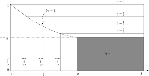
Figure 1: Level sets for the length exponent $\eta$ in the $(\delta,\gamma)$ plane consist of a rectangular block corresponding to the value $\eta=1$ and a family of lines starting vertically at the $\delta$-axis and turning horizontally upon hitting the graph given by $\delta\gamma=1$.

In Janssen, Prałat and Wilson JPW the empirical edge length distribution is studied for the model defined in Aiello . This is essentially the case of an affine function $f(k)=\gamma k+\beta$ and a profile function $\varphi(x)=p\mathbh{1}\{x<1/(2p)\}$, corresponding roughly to the case $\delta=\infty$. They show that if $\gamma>\frac{1}{2}$ and $\frac{3\gamma+2}{4\gamma+2}<\alpha<1$, then

$$\bigl{|}\bigl{\{}\mbox{edges of length longer than $t^{-\alpha}$}\bigr{\}}\bigr{|}\sim Ct^{(2-\alpha)+(({1}/\gamma)(\alpha-1))}$$

for an explicit constant $C>0$. Our result uses a different order of limits, but leads to the same order of growth for the comparable quantity $t\lambda[t^{1-\alpha},\infty)$. If $\gamma<\frac{1}{2}$ they show that the expected number of edges of length longer than $t^{-\alpha}$, for $0\leq\alpha<1$, grows of order $t^{\alpha}$, which is also of the same order as $t\lambda[t^{1-\alpha},\infty)$. Note that the general form of the profile functions allows for a genuinely richer phenomenology in our case.

4 Methods of proof

4.1 The rescaled picture

First, it is convenient to describe more explicitly the randomness involved in the “construction rule,” which determines the presence or absence of each edge in the network. To this end, denote by $\mathbb{T}_{1}\times(0,\infty)$ the set of potential vertices, and by

$$E\bigl{(}\mathbb{T}_{1}\times(0,\infty)\bigr{)}:=\bigl{\{}(\mathbf{y},\mathbf{x}),\mathbf{y},\mathbf{x}\in\mathbb{T}_{1}\times(0,\infty),\mathbf{y}\mbox{ younger than }\mathbf{x}\bigr{\}}$$

the set of potential edges. Introduce a family $\mathcal{V}$ of independent random variables, independent of $\mathcal{X}$, indexed by the set of potential edges and uniformly distributed on $[0,1]$. We will denote these variables by $\mathcal{V}_{\mathbf{x},\mathbf{y}}$ or $\mathcal{V}(\mathbf{x},\mathbf{y})$. A realization of $\mathcal{X}_{t}$ and $\mathcal{V}$ defines a network $G^{1}(\mathcal{X}_{t},\mathcal{V})$, with vertex set $\mathcal{X}_{t}$, obtained with the same construction as before, but with the construction rule replaced by the rule that you connect $\mathbf{x}$ to $\mathbf{y}$ if and only if

$$\mathcal{V}(\mathbf{x},\mathbf{y})\leq\varphi\biggl{(}\frac{sd(\mathbf{x},\mathbf{y})}{f(Z_{\mathbf{x}}(s-))}\biggr{)},$$ (3)

where $s$ is the birth time of the younger vertex $\mathbf{y}$. The growing networks $(G^{1}(\mathcal{X}_{t},\mathcal{V}))_{t>0}$ and $(G_{t})_{t>0}$ have the same law and will be identified. Moreover, the deterministic functional $G^{1}$ associates a graph structure to any set of points in $\mathbb{T}_{1}\times(0,\infty)$ and family of points in $[0,1]$ indexed by $E(\mathbb{T}_{1}\times(0,\infty))$.

Second, we want to generalize the construction, replacing $\mathbb{T}_{1}$ by $\mathbb{T}_{t}=\mathbb{R}/(t\mathbb{Z})$, the one-dimensional torus of length $t$. We permit the case $t=\infty$, with the convention $\mathbb{T}_{\infty}=\mathbb{R}$. The definition of the set of potential vertices $\mathbb{T}_{t}\times(0,\infty)$ and the set of potential edges $E(\mathbb{T}_{t}\times(0,\infty))$ is straightforward. We define the functional $G^{t}$, for $t\in(0,\infty]$, in analogy to the case $t=1$, by associating a graph structure to any set of points in $\mathbb{T}_{t}\times(0,\infty)$, and any family of values in $[0,1]$ indexed by $E(\mathbb{T}_{t}\times(0,\infty))$. In the construction, rule (3) is unchanged, but with the new understanding that the distances are now those in $\mathbb{T}_{t}$.

For finite $t$, we introduce the rescaling mapping

$$h_{t}\dvt\mathbb{T}_{1}\times(0,t] \to \mathbb{T}_{t}\times(0,1],$$

$$(x,s) \mapsto (tx,s/t)$$

which expands the space by a factor $t$, the time by a factor $1/t$. The mapping $h_{t}$ operates on the set $\mathcal{X}$, but also on $\mathcal{V}$, with

$$h_{t}(\mathcal{V})_{h_{t}(\mathbf{x}),h_{t}(\mathbf{y})}:=\mathcal{V}_{\mathbf{x},\mathbf{y}}.$$

The operation of $h_{t}$ preserves the rule (3), and it is therefore simple to verify that we have

$$G^{t}\bigl{(}h_{t}(\mathcal{X}_{t}),h_{t}(\mathcal{V})\bigr{)}=h_{t}\bigl{(}G^{1}(\mathcal{X}_{t},\mathcal{V})\bigr{)}=h_{t}(G_{t}),$$

that is, it is the same to construct the graph and then rescale the picture, or to first rescale the picture, then construct the graph on this rescaled picture. Observe also that $h_{t}(\mathcal{X}_{t})$ is a Poisson point process of intensity $1$ on $\mathbb{T}_{t}\times(0,1]$, while $h_{t}(\mathcal{V})$ is still an independent family of i.i.d. uniform random variables on $[0,1]$, indexed by $E(\mathbb{T}_{t}\times(0,1])$.

From now on, we denote by $\mathcal{X}$ a Poisson point process with intensity 1 on $\mathbb{R}\times(0,1]$, and $\mathcal{V}$ an independent family of i.i.d. uniform on $[0,1]$ random variables, indexed by $E(\mathbb{R}\times(0,1])$. For finite $t>0$, identify $(-t/2,t/2]$ and $\mathbb{T}_{t}$, and write $\mathcal{X}^{t}$ for the restriction of $\mathcal{X}$ to $\mathbb{T}_{t}\times(0,1]$, and $\mathcal{V}^{t}$ for the restriction of $\mathcal{V}$ to the indices in $E(\mathbb{T}_{t}\times(0,1])$. We write $G^{t}(\mathcal{X},\mathcal{V})$ for $G^{t}(\mathcal{X}^{t},\mathcal{V}^{t})$, and observe that this graph has the same law as $h_{t}(G_{t})$. However, the process $t\mapsto G^{t}(\mathcal{X},\mathcal{V})$ behaves very differently from the original process $t\mapsto G_{t}$. Indeed, in the original process, the degree of any fixed vertex grows like $t^{\gamma+o(1)}$ (see Lemma 8) and thus goes to $+\infty$. By contrast, for the graphs $G^{t}(\mathcal{X},\mathcal{V})$, the following result establishes convergence to the graph $G^{\infty}(\mathcal{X},\mathcal{V})$ as defined in the preceding paragraph.

Proposition 5.

(i) The graph $G^{\infty}(\mathcal{X},\mathcal{V})$ defined above is almost surely locally finite, in the sense that its vertices all have finite degrees.

(ii) The graph $G^{t}(\mathcal{X},\mathcal{V})$, almost surely, converges locally to $G^{\infty}(\mathcal{X},\mathcal{V})$, in the sense that for each $\mathbf{x}\in\mathcal{X}$, for large $t$, the neighbors of $\mathbf{x}$ in $G^{t}(\mathcal{X},\mathcal{V})$ and in $G^{\infty}(\mathcal{X},\mathcal{V})$ coincide.

As a direct consequence we obtain the following corollary.

Corollary 6.

Almost surely, for any $\mathbf{x}\in\mathcal{X}$ and each $n\geq 1$, the neighborhood of vertex $\mathbf{x}$ in the graphs $G^{t}(\mathcal{X},\mathcal{V})$ and $G^{\infty}(\mathcal{X},\mathcal{V})$ up to graph distance $n$ will coincide for large $t$.

The key to the understanding of the drastically different behavior of the graph-valued process $t\mapsto G^{t}(\mathcal{X},\mathcal{V})$ lies in the fact that a fixed vertex in this sequence of graphs has a birth time which is comparable to the age of the network. This age would be highly variable in time if mapped onto the original graph, but is kept constant in the process $t\mapsto G^{t}(\mathcal{X},\mathcal{V})$.

Regardless of the strength of Proposition 5, it only states a local convergence result and is therefore insufficient for our purpose. Global results require the introduction of a specific law of large numbers, which we state and prove now.

4.2 A general weak law of large numbers

For $x_{0}\in\mathbb{R}$, we introduce the translation

$$\theta_{x_{0}}\dvt\mathbb{R}\times(0,1] \to \mathbb{R}\times(0,1],$$

$$(x,s) \mapsto (x+x_{0},s).$$

The translation $\theta_{x_{0}}$ operates on $\mathbb{R}\times(0,1]$, and in a canonical manner also on the point sets in $\mathbb{R}\times(0,1]$, and on families indexed by $E(\mathbb{R}\times(0,1])$. Consider a functional $\xi_{\infty}$, which associates a nonnegative real number $\xi_{\infty}((x,s),\mathcal{Z},\mathcal{W})$ to a point set $\mathcal{Z}\subset\mathbb{R}\times(0,1]$ with a distinguished point $\mathbf{x}=(x,s)\in\mathcal{Z}$, and a family $\mathcal{W}$ of numbers in $[0,1]$ indexed by $E(\mathbb{R}\times(0,1])$. The functional is supposed to be translation invariant, in the sense that

$$\xi_{\infty}(\mathbf{x},\mathcal{Z},\mathcal{W})=\xi_{\infty}\bigl{(}\theta_{x_{0}}(\mathbf{x}),\theta_{x_{0}}(\mathcal{Z}),\theta_{x_{0}}(\mathcal{W})\bigr{)}.$$

Similarly, for each $t>0$, and $x_{0}\in\mathbb{T}_{t}$, we introduce the translation

$$\theta^{t}_{x_{0}}\dvt\mathbb{T}_{t}\times(0,1] \to \mathbb{T}_{t}\times(0,1],$$

$$(x,s) \mapsto (x+x_{0},s),$$

and we consider functionals $\xi_{t}$, which associate a nonnegative real number $\xi_{t}((x,s),\mathcal{Z},\mathcal{W})$ to a point set $\mathcal{Z}\subset\mathbb{T}_{t}\times(0,1]$ with a distinguished point $(x,s)\in\mathcal{Z}$ and a family $\mathcal{W}$ of numbers in $[0,1]$ indexed by $E(\mathbb{T}_{t}\times(0,1])$. The functionals $\xi_{t}$ are supposed to be invariant under the translations $\theta^{t}_{x_{0}}$.

Finally, for the sake of simplifying notation, we will also write $\xi_{\infty}(\mathbf{x},\mathcal{Z},\mathcal{W})$ for $\xi_{\infty}(\mathbf{x},\mathcal{Z}\cup\{\mathbf{x}\},\mathcal{W})$ when the set $\mathcal{Z}$ does not contain $\mathbf{x}$, and similarly $\xi_{t}(\mathbf{x},\mathcal{Z},\mathcal{W})$ for $\xi_{t}(\mathbf{x},\mathcal{Z}\cup\{\mathbf{x}\},\mathcal{W})$. We also write

$$\xi_{\infty}(\mathcal{Z},\mathcal{W}) := \int_{0}^{1}\xi_{\infty}\bigl{(}(0,s),\mathcal{Z},\mathcal{W}\bigr{)}\,\mathrm{d}s,$$

$$\xi_{t}(\mathcal{Z},\mathcal{W}) := \int_{0}^{1}\xi_{t}\bigl{(}(0,s),\mathcal{Z},\mathcal{W}\bigr{)}\,\mathrm{d}s.$$

Recall the notation of the Poisson point process $\mathcal{X}$ and of the family of random variables $\mathcal{V}$, as well as their restrictions $\mathcal{X}^{t}$ and $\mathcal{V}^{t}$. In the following theorem, $U$ denotes a random variable, uniform on $(0,1]$, and independent of the point process $\mathcal{X}$ and of $\mathcal{V}$.

Theorem 7 ((Weak law of large numbers)).

Suppose that the following two conditions hold: [(A)]

as $t\to\infty$, the random variable $\xi_{t}((0,U),\mathcal{X}^{t},\mathcal{V}^{t})$ converges in probability to the random variable $\xi_{\infty}((0,U),\mathcal{X},\mathcal{V})$;

for some $p>1$ we have the uniform moment condition

$$\sup_{t>0}\mathbb{E}\bigl{[}\xi_{t}\bigl{(}(0,U),\mathcal{X}^{t},\mathcal{V}^{t}\bigr{)}^{p}\bigr{]}<\infty.$$

Then, as $t\to\infty$, we have the following convergence in the $L^{1}$-sense:

$$\frac{1}{t}\sum_{\mathbf{x}\in\mathcal{X}^{t}}\xi_{t}\bigl{(}\mathbf{x},\mathcal{X}^{t},\mathcal{V}^{t}\bigr{)}\longrightarrow\mathbb{E}\bigl{[}\xi_{\infty}\bigl{(}(0,U),\mathcal{X},\mathcal{V}\bigr{)}\bigr{]}=\mathbb{E}\bigl{[}\xi_{\infty}(\mathcal{X},\mathcal{V})\bigr{]}.$$ (4)

Remark 5.

(i) Theorem 7 is an adaptation of Theorem 2.1 of Penrose and Yukich YukichPenrose to our purpose. Their result also includes a de-Poissonisation, but this is incompatible with our set-up because of the explicit time dependence of the attachment probabilities.

(ii) Suppose now that only condition (A) is satisfied. On the one hand, the proof still works if the family $(\xi_{t}((0,U),\mathcal{X}^{t},\mathcal{V}^{t}))_{t>0}$ is uniformly integrable. On the other hand, if $\mathbb{E}[\xi_{\infty}(\mathcal{X},\mathcal{V})]=\infty$, then, by applying the theorem to the bounded functional $\xi^{k}_{t}(\mathbf{x},\mathcal{Z},\mathcal{W}):=\xi_{t}(\mathbf{x},\mathcal{Z},\mathcal{W})\wedge k$ and letting $k$ go to $\infty$, we get the convergence in probability of

$$\frac{1}{t}\sum_{\mathbf{x}\in\mathcal{X}^{t}}\xi_{t}\bigl{(}\mathbf{x},\mathcal{X}^{t},\mathcal{V}^{t}\bigr{)}$$

to $+\infty$. The only case when the theorem does not yield any convergence result is when $\mathbb{E}[\xi_{\infty}(\mathcal{X},\mathcal{V})]$ is finite, but the family $(\xi_{t}((0,U),\mathcal{X}^{t},\mathcal{V}^{t}))_{t>0}$ fails to be uniformly integrable.

As in Theorem 2.1 in YukichPenrose the proof relies on a first moment calculation, and then a second moment calculation which is performed under a stronger uniform moment condition, and finally a step to allow the removal of this extra condition.

First moment: We compute, by Campbell’s formula,

$$\mathbb{E}\biggl{[}\frac{1}{t}\sum_{\mathbf{x}\in\mathcal{X}^{t}}\xi_{t}\bigl{(}\mathbf{x},\mathcal{X}^{t},\mathcal{V}^{t}\bigr{)}\biggr{]} = \int_{\mathbb{T}_{t}\times(0,1]}\frac{\mathrm{d}x\,\mathrm{d}s}{t}\mathbb{E}\bigl{[}\xi_{t}\bigl{(}(x,s),\mathcal{X}^{t},\mathcal{V}^{t}\bigr{)}\bigr{]}$$

$$= \int_{0}^{1}\mathrm{d}s\,\mathbb{E}\bigl{[}\xi_{t}\bigl{(}(0,s),\mathcal{X}^{t},\mathcal{V}^{t}\bigr{)}\bigr{]}$$

$$= \mathbb{E}\bigl{[}\xi_{t}\bigl{(}(0,U),\mathcal{X}^{t},\mathcal{V}^{t}\bigr{)}\bigr{]}.$$

Note that in all these expressions but the first one, a point is added to $\mathcal{X}^{t}$. The second equality follows from the spatial invariance by the translation $\theta_{-x}^{t}$, both of the functional $\xi_{t}$ and of the law of $(\mathcal{X}^{t},\mathcal{V}^{t})$. Now condition (A) states that the variables $\xi_{t}((0,U),\mathcal{X}^{t},\mathcal{V}^{t})$ converge in probability to $\xi_{\infty}((0,U),\mathcal{X},\mathcal{V})$. Condition (B) ensures that they are uniformly integrable. Therefore we have convergence of the expectations $\mathbb{E}[\xi_{t}((0,U),\mathcal{X}^{t},\mathcal{V}^{t})]$ to $\mathbb{E}[\xi_{\infty}((0,U),\mathcal{X},\mathcal{V})]$, and this expectation is finite.

Second moment: We work here under the stronger assumption that the uniform moment condition holds for some $p>2$. Similarly as in the case of the first moment, we get

$$\mathbb{E}\biggl{[}\biggl{(}\frac{1}{t}\sum_{\mathbf{x}\in\mathcal{X}^{t}}\xi_{t}\bigl{(}\mathbf{x},\mathcal{X}^{t},\mathcal{V}^{t}\bigr{)}\biggr{)}^{2}\biggr{]}$$

$$\qquad=\mathbb{E}\biggl{[}\frac{1}{t^{2}}\sum_{\mathbf{x}\in\mathcal{X}^{t}}\xi_{t}\bigl{(}\mathbf{x},\mathcal{X}^{t},\mathcal{V}^{t}\bigr{)}^{2}\biggr{]}+\mathbb{E}\biggl{[}\frac{1}{t^{2}}\mathop{\sum_{\mathbf{x},\mathbf{x}^{\prime}\in\mathcal{X}^{t}}}_{\mathbf{x}\neq\mathbf{x}^{\prime}}\xi_{t}\bigl{(}\mathbf{x},\mathcal{X}^{t},\mathcal{V}^{t}\bigr{)}\xi_{t}\bigl{(}\mathbf{x}^{\prime},\mathcal{X}^{t},\mathcal{V}^{t}\bigr{)}\biggr{]}$$

$$\qquad=\frac{1}{t}\mathbb{E}\bigl{[}\xi_{t}\bigl{(}(X_{1},U_{1}),\mathcal{X}^{t},\mathcal{V}^{t}\bigr{)}^{2}\bigr{]}$$

$$\quad\qquad{}+\mathbb{E}\bigl{[}\xi_{t}\bigl{(}(tX_{1},U_{1}),\mathcal{X}^{t}\cup\bigl{\{}(tX_{2},U_{2})\bigr{\}},\mathcal{V}^{t}\bigr{)}$$

$$\hskip 54.0pt{}\times\xi_{t}\bigl{(}(tX_{2},U_{2}),\mathcal{X}^{t}\cup\bigl{\{}(tX_{1},U_{1})\bigr{\}},\mathcal{V}^{t}\bigr{)}\bigr{]},$$

with $X_{1}$ and $X_{2}$ uniform in $\mathbb{T}_{1}$, $U_{1}$ and $U_{2}$ uniform in $(0,1)$, and $\mathcal{X}$, $X_{1}$, $U_{1}$, $X_{2}$, $U_{2}$ independent. The first term goes to zero, thanks to the uniform moment condition with $p>2$ ($p=2$ would be enough).

Now, the second term is the expectation of the following product of random variables:

$$\xi_{t}\bigl{(}(0,U_{1}),\theta^{t}_{-tX_{1}}\bigl{(}\mathcal{X}^{t}\bigr{)}\cup\bigl{\{}\bigl{(}t(X_{2}-X_{1}),U_{2}\bigr{)}\bigr{\}},\theta^{t}_{-tX_{1}}\bigl{(}\mathcal{V}^{t}\bigr{)}\bigr{)}$$

(5)

$$\quad{}\times\xi_{t}\bigl{(}(0,U_{2}),\theta^{t}_{-tX_{2}}\bigl{(}\mathcal{X}^{t}\bigr{)}\cup\bigl{\{}\bigl{(}t(X_{1}-X_{2}),U_{1}\bigr{)}\bigr{\}},\theta^{t}_{-tX_{2}}\bigl{(}\mathcal{V}^{t}\bigr{)}\bigr{)},$$

whose behavior we have to understand. We first concentrate on the first term. Write

$$\widetilde{\mathcal{X}}^{t}:=\theta^{t}_{-tX_{1}}\bigl{(}\mathcal{X}^{t}\bigr{)}\cup\bigl{\{}\bigl{(}t(X_{2}-X_{1}),U_{2}\bigr{)}\bigr{\}},\qquad\widetilde{\mathcal{V}}^{t}:=\theta^{t}_{-tX_{1}}\bigl{(}\mathcal{V}^{t}\bigr{)}.$$

We introduce three events, $E_{t}:=\{td(X_{1},X_{2})>\sqrt{t}\}$, $F_{t}:=\{td(X_{1},1/2)>\sqrt{t}/2\}$ and $G_{t}$ the event that the Poisson point process $\mathcal{X}^{t}$ has at least one point in $\{(x,s)\dvtx d(x,0)>\sqrt{t}\}$. These are all asymptotically almost sure (a.a.s.), in the sense that their probability goes to one when $t\to\infty$. We make two important observations:

• On the event $E_{t}\cap F_{t}$, the restrictions to $\mathbb{T}_{\sqrt{t}}\times(0,1]$ of the sets $\widetilde{\mathcal{X}}^{t}$ and $\theta_{-tX_{1}}(\mathcal{X})$ coincide. Similarly, the restrictions to $\mathbb{T}_{\sqrt{t}}\times(0,1]$ of the families $\widetilde{\mathcal{V}}^{t}$ and $\theta_{-tX_{1}}(\mathcal{V})$ also coincide.

• The law of $(\widetilde{\mathcal{X}}^{t},\widetilde{\mathcal{V}}^{t})$ knowing $E_{t}$ equals the law of $(\mathcal{X}^{t},\mathcal{V}^{t})$ knowing $G_{t}$.

These observations allow the following calculation, with $\eta$ some positive real number. Note that we will apply now (and until the end of this proof) the functional $\xi_{\sqrt{t}}$ to point sets on $\mathbb{R}\times(0,1]$ or $\mathbb{T}_{t}\times(0,1]$ (and families indexed by $E(\mathbb{R}\times(0,1])$ or $E(\mathbb{T}_{t}\times(0,1])$). This is only to lighten the notation a bit. It should always be understood that the functional is applied to the restrictions on $\mathbb{T}_{\sqrt{t}}\times(0,1]$.

$$\limsup_{t\to\infty}\mathbb{P}\bigl{\{}\bigl{|}\xi_{t}\bigl{(}(0,U_{1}),\widetilde{\mathcal{X}}^{t},\widetilde{\mathcal{V}}^{t}\bigr{)}-\xi_{\sqrt{t}}\bigl{(}(0,U_{1}),\theta_{-tX_{1}}(\mathcal{X}),\theta_{-tX_{1}}(\mathcal{V})\bigr{)}\bigr{|}>\eta\bigr{\}}$$

$$\qquad=\limsup_{t\to\infty}\mathbb{E}\bigl{[}\mathbh{1}\bigl{\{}\bigl{|}\xi_{t}\bigl{(}(0,U_{1}),\widetilde{\mathcal{X}}^{t},\widetilde{\mathcal{V}}^{t}\bigr{)}$$

$$\hskip 88.0pt{}-\xi_{\sqrt{t}}\bigl{(}(0,U_{1}),\theta_{-tX_{1}}(\mathcal{X}),\theta_{-tX_{1}}(\mathcal{V})\bigr{)}\bigr{|}>\eta\bigr{\}}\mathbh{1}_{F_{t}}|E_{t}\bigr{]}$$

$$\qquad=\limsup_{t\to\infty}\mathbb{E}\bigl{[}\mathbh{1}\bigl{\{}\bigl{|}\xi_{t}\bigl{(}(0,U_{1}),\widetilde{\mathcal{X}}^{t},\widetilde{\mathcal{V}}^{t}\bigr{)}-\xi_{\sqrt{t}}\bigl{(}(0,U_{1}),\widetilde{\mathcal{X}}^{t},\widetilde{\mathcal{V}}^{t}\bigr{)}\bigr{|}>\eta\bigr{\}}\mathbh{1}_{F_{t}}|E_{t}\bigr{]}$$

$$\qquad=\limsup_{t\to\infty}\mathbb{E}\bigl{[}\mathbh{1}\bigl{\{}\bigl{|}\xi_{t}\bigl{(}(0,U_{1}),\mathcal{X}^{t},\mathcal{V}^{t}\bigr{)}-\xi_{\sqrt{t}}\bigl{(}(0,U_{1}),\mathcal{X}^{t},\mathcal{V}^{t}\bigr{)}\bigr{|}>\eta\bigr{\}}\mathbh{1}_{F_{t}}|G_{t}\bigr{]}$$

$$\qquad=\limsup_{t\to\infty}\mathbb{P}\bigl{\{}\bigl{|}\xi_{t}\bigl{(}(0,U_{1}),\mathcal{X}^{t},\mathcal{V}^{t}\bigr{)}-\xi_{\sqrt{t}}\bigl{(}(0,U_{1}),\mathcal{X}^{t},\mathcal{V}^{t}\bigr{)}\bigr{|}>\eta\bigr{\}}=0.$$

The last equality uses condition (A). Hence, the variable

$$\xi_{t}\bigl{(}(0,U_{1}),\widetilde{\mathcal{X}}^{t},\widetilde{\mathcal{V}}^{t}\bigr{)}-\xi_{\sqrt{t}}\bigl{(}(0,U_{1}),\theta_{-tX_{1}}(\mathcal{X}),\theta_{-tX_{1}}(\mathcal{V})\bigr{)}$$

converges in probability to zero. Similarly, one can see that the variable

$$\xi_{t}\bigl{(}(0,U_{2}),\theta^{t}_{-tX_{2}}\bigl{(}\mathcal{X}^{t}\bigr{)}\cup\bigl{\{}\bigl{(}t(X_{1}-X_{2}),U_{1}\bigr{)}\bigr{\}},\theta^{t}_{-tX_{2}}\bigl{(}\mathcal{V}^{t}\bigr{)}\bigr{)}$$

$$\quad{}-\xi_{\sqrt{t}}\bigl{(}(0,U_{2}),\theta_{-tX_{2}}(\mathcal{X}),\theta^{t}_{-tX_{2}}(\mathcal{V})\bigr{)}$$

converges in probability to zero. Next, observe that the two variables

$$\xi_{\sqrt{t}}\bigl{(}(0,U_{1}),\theta_{-tX_{1}}(\mathcal{X}),\theta_{-tX_{1}}(\mathcal{V})\bigr{)}$$

and

$$\xi_{\sqrt{t}}\bigl{(}(0,U_{2}),\theta_{-tX_{2}}(\mathcal{X}),\theta_{-tX_{2}}(\mathcal{V})\bigr{)}$$

are independent conditionally on the event $E_{t}$. Moreover, observe that the law of each one converges to that of $\xi_{\infty}((0,U_{1}),\mathcal{X},\mathcal{V})$, thanks to condition (A) again. Gathering the results, we get that the product in (4.2) converges in law to the product of two independent copies of $\xi_{\infty}((0,U_{1}),\mathcal{X},\mathcal{V})$.

Finally, use Cauchy–Schwarz to get a uniform moment condition for this product for $\frac{p}{2}>1$. Hence the expectation of the product goes to $\mathbb{E}[\xi_{\infty}((0,U_{1}),\break\mathcal{X},\mathcal{V})]^{2}$. Therefore we get (4), with convergence even in $L^{2}$.

Relaxing the moment condition: We finally work under the assumptions of the theorem, that is, the uniform moment condition is satisfied only for some $p>1$. Introduce the bounded functional

$$\xi^{k}_{t}(\mathbf{x},\mathcal{Z},\mathcal{W}):=\xi_{t}(\mathbf{x},\mathcal{Z},\mathcal{W})\wedge k.$$

This functional clearly satisfies condition (A) and the uniform moment condition for any $p$, in particular for some $p>2$. Therefore, we get the convergence of

$$\frac{1}{t}\sum_{\mathbf{x}\in\mathcal{X}^{t}}\xi_{t}^{k}\bigl{(}\mathbf{x},\mathcal{X}^{t},\mathcal{V}^{t}\bigr{)}$$

to $\mathbb{E}[\xi_{\infty}((0,U_{1}),\mathcal{X},\mathcal{V})\wedge k]$, in $L^{2}$, and thus in $L^{1}$. Now note that

$$\mathbb{E}\biggl{[}\frac{1}{t}\sum_{(x,s)\in\mathcal{X}^{t}}\bigl{(}\xi_{t}\bigl{(}(x,s),\mathcal{X}^{t},\mathcal{V}^{t}\bigr{)}-\xi_{t}^{k}\bigl{(}(x,s),\mathcal{X}^{t},\mathcal{V}^{t}\bigr{)}\bigr{)}\biggr{]}$$

$$\qquad=\mathbb{E}\bigl{[}\xi_{t}\bigl{(}(0,U),\mathcal{X}^{t},\mathcal{V}^{t}\bigr{)}-\xi_{t}^{k}\bigl{(}(0,U),\mathcal{X}^{t},\mathcal{V}^{t}\bigr{)}\bigr{]},$$

which is nonnegative and goes uniformly to zero for $k\to\infty$, as the variables $\xi_{t}((0,U),\mathcal{X}^{t},\mathcal{V}^{t})$ are uniformly integrable, by the uniform moment condition. It follows that

$$\frac{1}{t}\sum_{\mathbf{x}\in\mathcal{X}^{t}}\xi_{t}\bigl{(}\mathbf{x},\mathcal{X}^{t},\mathcal{V}^{t}\bigr{)}$$

converges in $L^{1}$ to the limit of $\mathbb{E}[\xi_{\infty}((0,U),\mathcal{X},\mathcal{V})\wedge k]$, that is $\mathbb{E}[\xi_{\infty}((0,U),\break\mathcal{X},\mathcal{V})]$.

4.3 A bound on the indegree and on the linking probability

As we consider various graphs on various spaces, we need to introduce more flexible notation for the degrees. If $G$ is a graph with vertices in $\mathbb{T}_{t}\times(0,\infty)$ we write $\mathbf{x}\leftrightarrow\mathbf{y}$ to indicate that there is an edge between the vertices $\mathbf{x}$ and $\mathbf{y}$. If $\mathbf{x}_{0}=(x_{0},s_{0})$ is in $G$, then, for any $s\geq s_{0}$, we define

$$Z_{\mathbf{x}_{0}}(s,G)=\bigl{|}\bigl{\{}(x,r)\in G\dvtx(x,r)\leftrightarrow(x_{0},s_{0}),s_{0}<r\leq s\bigr{\}}\bigr{|},$$

the indegree of $\mathbf{x}_{0}$ in $G$ “at time $s$” and

$$Y_{\mathbf{x}_{0}}(G)=\bigl{|}\bigl{\{}(x,r)\in G\dvtx(x,r)\leftrightarrow(x_{0},s_{0}),r<s_{0}\bigr{\}}\bigr{|},$$

its outdegree. For $t\in(0,\infty]$ and for $0<s_{0}\leq s\leq 1$, we write

$$Z^{t}_{\mathbf{x}_{0}}(s)=Z_{\mathbf{x}_{0}}\bigl{(}s,G^{t}\bigl{(}\mathcal{X}\cup\{\mathbf{x}_{0}\},\mathcal{V}\bigr{)}\bigr{)}\quad\mbox{and}\quad Y^{t}_{\mathbf{x}_{0}}=Y_{\mathbf{x}_{0}}\bigl{(}G^{t}\bigl{(}\mathcal{X}\cup\{\mathbf{x}_{0}\},\mathcal{V}\bigr{)}\bigr{)}.$$

For fixed $t$ and $\mathbf{x}_{0}$, call $(Z^{t}_{\mathbf{x}_{0}}(s))_{s_{0}\leq s\leq 1}$ the indegree process. In this part only, we extend the Poisson point process $\mathcal{X}$ on the whole $\mathbb{R}\times(0,\infty)$, and allow any $0<s_{0}\leq s$ in the definition of $Z^{t}_{\mathbf{x}_{0}}(s)$. For $\mathbf{x}_{0}\in\mathbb{T}_{1}\times(0,\infty)$, the process $(Z^{1}_{\mathbf{x}_{0}}(s))_{s\geq s_{0}}$ has the same law as the process $(Z_{\mathbf{x}_{0}}(s))_{s\geq s_{0}}$ introduced earlier in Section 2, so that the results of this part apply simultaneously for the rescaled graphs and for the unrescaled ones. Now, observe that the law of the indegree process does not depend on the spatial position $x_{0}\in\mathbb{T}_{t}$. Therefore, we simply write $Z^{t}_{s_{0}}(s)$ for $Z^{t}_{(0,s_{0})}(s)$ and $Y^{t}_{s_{0}}$ for $Y^{t}_{(0,s_{0})}$. If $\mathbf{x}$ and $\mathbf{y}$ are two vertices in $\mathcal{X}$, we write $\mathbf{x}\mathop{\leftrightarrow}\limits_{t}\mathbf{y}$ for the event that $\mathbf{x}$ and $\mathbf{y}$ are linked in $G^{t}(\mathcal{X},\mathcal{V})$.

Lemma 8.

For all $t>0$ and $\mathbf{x}_{0}\in\mathbb{T}_{t}$, we have almost surely

$$\ln Z^{t}_{\mathbf{x}_{0}}(s)\sim\gamma\ln s\qquad\mbox{as }s\to\infty.$$

This lemma confirms that the degree of a fixed vertex in the unrescaled graphs grows polynomially of order $\gamma>0$, and in particular that it explodes. Before proving it we give a bound on the probability that a vertex reaches an exceptionally high degree, allowing it to be connected to an exceptionally distant vertex. Exponential bounds, uniform in $t$, are provided in the following lemma and its corollary. For the sake of simplicity, they are only stated in the case of a linear function $f$. We refer to Remark 6 for the general case.

Lemma 9.

Suppose $f(k)=\gamma k+\beta$, with $\gamma\in(0,1)$ and $\beta>0$. Let $p=\lceil\frac{\beta}{\gamma}-1\rceil$, so that $f(k)\leq\gamma(k+p+1)$. For any $t\in(0,\infty]$, any $s_{0}<s\leq 1$ and any $k\geq 0$, the following inequality holds:

$$\mathbb{P}\bigl{\{}Z^{t}_{s_{0}}(s)\geq k\bigr{\}}\leq e^{{p}/4}\exp\biggl{(}-\frac{k}{8}\biggl{(}\frac{s_{0}}{s}\biggr{)}^{\gamma}\biggr{)}.$$ (6)

Corollary 10.

Under the assumptions of Lemma 9, define the inverse of the profile function $\varphi$ by

$$\varphi^{-1}(u):=\inf\bigl{\{}x>0\dvtx\varphi(x)<u\bigr{\}}.$$

Then there is a constant $c$ depending only on $f$, such that for any $t\in(0,\infty]$ and any $(x,s)\in\mathbb{R}\times(0,1]$, we have

$$\mathbb{P}\bigl{\{}(0,1)\mathop{\leftrightarrow}\limits_{t}(x,s)|(0,1)\in\mathcal{X},(x,s)\in\mathcal{X},\mathcal{V}_{(0,1),(x,s)}=u\bigr{\}}$$

(7)

$$\qquad\leq c\exp\biggl{(}-\frac{|x|s^{\gamma}}{8\gamma\varphi^{-1}(u)}\biggr{)}.$$

Remark 6.

In the nonlinear case, we can first bound $f$ from above by a linear function, then, by an easy stochastic domination argument, get the inequalities of the lemma and its corollary with the linear bound instead of $f$. We get almost equally good bounds. More precisely, for any $\gamma^{\prime}>\gamma$, we can find $\beta^{\prime}>0$ such that $f(k)\leq\gamma^{\prime}k+\beta^{\prime}$ for any natural number $k$, and we thus get bounds for any exponent $\gamma^{\prime}>\gamma$.

A first corollary of Lemma 9 is that the indegree $Z^{t}_{\mathbf{x}_{0}}(s)$ is always almost surely finite, even when $t=\infty$. The same holds for the outdegree; see Proposition 13 below.

At this stage, let us discuss the important monotonicity property. If we fix $s_{0}$ and $s$ and let $t$ grow to $+\infty$, then $Z^{t}_{s_{0}}(s)$ will grow and converge to $Z^{\infty}_{s_{0}}(s)$. Moreover, if we change the position of the vertex to be nonzero, we do not change the law of its indegree and therefore its indegree will still be stochastically increasing in $t$ and stochastically dominated by $Z^{\infty}_{s_{0}}(s)$. By contrast, no such property holds for the outdegree. Indeed, increasing $t$ may increase the distance of two vertices near opposite ends of the boundary of $[-\frac{t}{2},\frac{t}{2}]$, thus decreasing the indegree of the younger vertex which, in turn, might destroy further links, eventually reducing the outdegree of the vertex at the origin.

Proof of Lemma 8 We fix $s_{0}>0$ and start with the case $t=\infty$. The indegree process $(Z^{\infty}_{s_{0}}(s))_{s>s_{0}}$ is an time-inhomogeneous pure birth process, starting from $Z^{\infty}_{s_{0}}(s_{0})=0$, and for which, at time $s$, the transition density from state $k$ to state $k+1$ is $f(k)/s$. Indeed, given $Z_{s_{0}}(s)=k$, we have $Z^{\infty}_{s_{0}}(s+\mathrm{d}s)\geq k+1$ if and only if the set

$$\biggl{\{}(y,u)\in\mathcal{X}\dvtx u\in(s,s+\mathrm{d}s],\mathcal{V}\bigl{(}(0,1),(y,u)\bigr{)}\leq\varphi\biggl{(}\frac{ud(y,0)}{f(k)}\biggr{)}\biggr{\}}$$

is nonempty, which due to the normalization of $\varphi$ happens with probability $\frac{f(k)}{s}\,\mathrm{d}s+o(\mathrm{d}s)$. We introduce a logarithmic change of time and write

$$\widetilde{Z}(u):=Z^{\infty}_{s_{0}}\bigl{(}s_{0}e^{u}\bigr{)}.$$

Then the process $\widetilde{Z}$ is a time-homogeneous pure birth process, with jumping intensity from state $k$ to state $k+1$ equal to $f(k)$. Write $T_{k}:=\inf\{u\dvtx\widetilde{Z}(u)\geq k\}$ for the first time when this process hits state $k$, which is finite as $f$ is nondecreasing. Then $(T_{i+1}-T_{i})_{i\geq 0}$ are independent, and $T_{i+1}-T_{i}$ is exponential with parameter $f(i)$. The process

$$M_{k}:=T_{k}-\sum_{i=0}^{k-1}\frac{1}{f(i)}$$

is a martingale, which is bounded in $L^{2}$ and thus convergent. Hence, we have $T_{k}\sim\frac{1}{\gamma}\ln k$, and further

$$\ln\widetilde{Z}(u)\sim\gamma u\quad\mbox{and}\quad\ln Z^{\infty}_{s_{0}}(s)\sim\gamma\ln s.$$

For the case of a finite $t$, we first get, from the monotonicity property, the upper bound

$$\limsup_{s\to\infty}\frac{\ln Z^{t}_{s_{0}}(s)}{\ln s}\leq\gamma.$$

In particular, a.s., we have $Z^{t}_{s_{0}}(s)\leq s^{(1+\gamma)/2}$ for $s$ large enough. But the process $(Z^{t}_{s_{0}}(s))_{s>s_{0}}$ is a time-inhomogeneous pure birth process with transition density from state $k$ to state $k+1$

$$2f(k)\int_{0}^{({st})/({f(k)})}\varphi(y)\,\mathrm{d}y,$$

which is equivalent to $f(k)$ when $t\uparrow\infty$, uniformly for all $s$ and $k\leq s^{(1+\gamma)/2}$. The same arguments as in the case $t=\infty$ then yield the lower bound, showing that we still have $\ln Z^{t}_{s_{0}}(s)\sim\gamma\ln s$.

Proof of Lemma 9 By the monotonicity argument we can suppose $t=\infty$ and, as before, we study the chain $\widetilde{Z}$ and its hitting times $T_{k}$. The parameter of the exponential variable $T_{i+1}-T_{i}$ is $f(i)$, which is less than or equal to $(p+i+1)\gamma$. It follows that $T_{k}$ (!!CHANGE!!) dominates stochastically a sum of independent exponential random variables with parameters $(p+1)\gamma$, $(p+2)\gamma,\ldots,(p+k)\gamma$, respectively.

Let $(\tilde{\tau}_{i})_{1\leq i\leq k+p}$ be a family of i.i.d. random variables, each following an exponential law with the same parameter $\gamma$. Let $(\tilde{\tau}_{i_{1}},\tilde{\tau}_{i_{2}},\ldots,\tilde{\tau}_{i_{k+p}})$ denote their decreasing rearrangement, and $\tilde{\tau}_{i_{k+p+1}}=0$. For $1\leq j\leq k+p$, let $\tau_{j}=\tilde{\tau}_{i_{j}}-\tilde{\tau}_{i_{j+1}}$. Then the family $(\tau_{j})_{1\leq j\leq k+p}$ is independent, and $\tau_{j}$ is an exponential variable with parameter $j\gamma$. Observe also that

$$\tau_{p+1}+\cdots+\tau_{p+k}=\tilde{\tau}_{i_{p+1}}.$$

Hence,

$$\mathbb{P}\bigl{\{}Z^{\infty}_{s_{0}}\bigl{(}s_{0}e^{u}\bigr{)}\geq k\bigr{\}}\leq\mathbb{P}\{\tilde{\tau}_{i_{p+1}}\leq u\}.$$

Now write

$$\{\tilde{\tau}_{i_{p+1}}\leq u\}=\Biggl{\{}\sum_{j=1}^{k+p}\mathbh{1}\{\tilde{\tau}_{j}>u\}\leq p\Biggr{\}}.$$

The sum of indicators follows a binomial law of parameters $k+p$ and $\exp(-\gamma u)$. Recall the concentration inequality for binomial random variables $X$,

$$\mathbb{P}\bigl{\{}X\leq\mathbb{E}[X]-\lambda\bigr{\}}\leq\exp\biggl{(}-\frac{\lambda^{2}}{2\mathbb{E}[X]}\biggr{)}.$$

We apply this with $\lambda=\frac{1}{2}(k+p)\exp(-\gamma u)$ and get

$$\mathbb{P}\Biggl{\{}\sum_{j=1}^{k+p}\mathbh{1}\{\tilde{\tau}_{j}>u\}\leq p\Biggr{\}} \leq \exp\biggl{(}-\frac{k}{8}e^{-\gamma u}\biggr{)}\mathbh{1}\bigl{\{}2p\leq ke^{-\gamma u}\bigr{\}}+\mathbh{1}\bigl{\{}2p>ke^{-\gamma u}\bigr{\}}$$

$$\leq \exp(p/4)\exp\biggl{(}-\frac{k}{8}e^{-\gamma u}\biggr{)}.$$

Finally, gathering the results, and taking $u=\ln s-\ln s_{0}$ gives, for any $k\geq 0$,

$$\mathbb{P}\bigl{\{}Z^{\infty}_{s_{0}}(s)\geq k\bigr{\}}\leq\exp(p/4)\exp\biggl{(}-\frac{k}{8}\biggl{(}\frac{s_{0}}{s}\biggr{)}^{\gamma}\biggr{)},$$

as required.

Proof of Corollary 10 The event $(0,1)\mathop{\leftrightarrow}\limits_{t}\mathbf{x}$ coincides with the event that the indegree of vertex $\mathbf{x}$ at time one is large enough to ensure that the linking condition is satisfied. This indegree has the same law as $Z^{t}_{s}(1)$ and is independent of $\mathcal{V}((0,1),\mathbf{x})$. We thus get

$$\mathbb{P}\bigl{\{}(0,1)\mathop{\leftrightarrow}\limits_{t}\mathbf{x}|(0,1)\in\mathcal{X},\mathbf{x}\in\mathcal{X},\mathcal{V}\bigl{(}(0,1),\mathbf{x}\bigr{)}=u\bigr{\}}$$

$$\qquad\leq\mathbb{P}\biggl{\{}\varphi\biggl{(}\frac{|x|}{f(Z^{t}_{s}(1))}\biggr{)}\geq u\biggr{\}}$$

$$\qquad\leq\mathbb{P}\biggl{\{}Z^{t}_{s}(1)\geq f^{-1}\biggl{(}\frac{|x|}{\varphi^{-1}(u)}\biggr{)}\biggr{\}}$$

$$\qquad\leq e^{p/4}\exp\biggl{(}-\frac{s^{\gamma}}{8}\biggl{(}\frac{|x|}{\gamma\varphi^{-1}(u)}-\frac{\beta}{\gamma}\biggr{)}\biggr{)}$$

$$\qquad\leq e^{(p/4)+(\beta/(8\gamma))}\exp\biggl{(}-\frac{|x|s^{\gamma}}{8\gamma\varphi^{-1}(u)}\biggr{)},$$

yielding (10) with the explicit constant $c=e^{(p/4)+(\beta/(8\gamma))}$.

5 Specific proofs of the main results

All the proofs of this section rely on the application of Theorem 7 to appropriate functionals. The functionals we use are only defined and used within each subsection. That is, the same notation in different subsections indicates different functionals.

5.1 Empirical indegree distribution

The following lemma provides the expected indegree of a vertex in the infinite graph with age uniform on $(0,1]$.

Lemma 11.

Let $U$ be uniformly distributed in $(0,1]$ and independent of the point process $\mathcal{X}$. Then, for any $k\geq 0$, we have

$$\mathbb{P}\bigl{\{}Z^{\infty}_{U}(1)=k\bigr{\}}=\mu(k),$$

where $\mu$ is the probability measure defined by

$$\mu(k)=\frac{1}{1+f(k)}\prod_{l=0}^{k-1}\frac{f(l)}{1+f(l)}.$$ (8)

Recall that the process $(Z^{\infty}_{s_{0}}(s_{0}e^{u}))_{0\leq u\leq\ln(1/s_{0})}$ is a time-homogeneous pure birth process with transition intensity from state $k$ to state $k+1$ equal to $f(k)$. Consider also the Markov chain $(\widehat{Z}_{u})_{0\leq u\leq\ln(1/s_{0})}$ with values in $[s_{0},1]\times\mathbb{N}\cup\{0\}$ started in $\widehat{Z}_{0}=(s_{0},0)$, such that at time $u$ the jumping intensity from state $(s,k)$ to state $(s,k+1)$ equals $f(k)$, and from state $(s,k)$ to state $(s_{0}e^{u},0)$ equals one.

The following facts are easy to check: [(3)]

The first coordinate $\widehat{Z}_{\ln(1/s_{0})}^{1}$ of the chain $(\widehat{Z}_{u})_{0\leq u\leq\ln(1/s_{0})}$ at time $\ln(1/s_{0})$ is equal to $s_{0}$ with probability $s_{0}$ and otherwise uniformly distributed on the interval $[s_{0},1]$.

Conditionally on $\widehat{Z}_{\ln(1/s_{0})}^{1}=s_{1}$, the second coordinate $\widehat{Z}_{\ln(1/s_{0})}^{2}$ has the same law as the random variable $Z^{\infty}_{s_{1}}(1)$.

The second coordinate $(\widehat{Z}^{2}_{u})_{0\leq u\leq\ln(1/s_{0})}$ is a time-homogeneous Markov chain, jumping from $k$ to $k+1$ with intensity $f(k)$, and from $k$ to zero with intensity one. The Markov chain stated in the third point was already encountered in DMdegrees . It is recurrent and its law converges to its invariant measure, which is precisely $\mu$. From the first two points, we deduce that the law of $\widehat{Z}_{\ln 1/s_{0}}^{2}$ conditional on $\widehat{Z}_{\ln 1/s_{0}}^{1}\neq s_{0}$ is the same as the law of $Z^{\infty}_{U}(t)$, where $U$ is uniform on $[s_{0},1]$. Now, letting $s_{0}$ go to zero gives the result.

Proof of Theorem 1 Let $g$ be a nondecreasing functional satisfying $\langle\mu,g^{p}\rangle<\infty$ for some $p>1$. We will apply Theorem 7 with the functionals $\xi_{t}(\mathbf{x},\mathcal{Z},\mathcal{W}):=g(Z_{\mathbf{x}}(1,G^{t}(\mathcal{Z}\cup\{\mathbf{x}\},\mathcal{W})))$, $t\in(0,\infty]$, so that for $\mathbf{x}\in\mathcal{X}^{t}$, we have $\xi_{t}(\mathbf{x},\mathcal{X},\mathcal{V})=g(Z^{t}_{\mathbf{x}}(1))$.

First, observe that the expectation of $\xi_{\infty}(\mathcal{X},\mathcal{V})$ is $\langle\mu,g\rangle$. Second, observe the following two simple consequences of the monotonicity property. The process $(Z^{t}_{U}(1))_{t>0}$ is nondecreasing and converges almost surely to $Z^{\infty}_{U}(1)$, which is finite almost surely. Moreover, the following uniform moment condition is satisfied:

$$\sup_{t>0}\mathbb{E}\bigl{[}\xi_{t}\bigl{(}(0,U),\mathcal{X},\mathcal{V}\bigr{)}^{p}\bigr{]}\leq\mathbb{E}\bigl{[}\xi_{\infty}\bigl{(}(0,U),\mathcal{X},\mathcal{V}\bigr{)}^{p}\bigr{]}=\bigl{\langle}\mu,g^{p}\bigr{\rangle}<\infty.$$

Hence, Theorem 7 ensures the convergence

$$\frac{1}{t}\sum_{\mathbf{x}\in\mathcal{X}^{t}}g\bigl{(}Z_{\mathbf{x}}^{t}(1)\bigr{)}\longrightarrow\langle\mu,g\rangle,$$

in $L^{1}$ and thus in probability. Combining this with the well-known convergence ${|\mathcal{X}^{t}|}/t\to 1$ gives the convergence in probability

$$\frac{1}{|\mathcal{X}^{t}|}\sum_{\mathbf{x}\in\mathcal{X}^{t}}g\bigl{(}Z_{\mathbf{x}}^{t}(1)\bigr{)}\longrightarrow\langle\mu,g\rangle,$$

and thus proves Theorem 1.

We close this subsection with a lemma which implies Proposition 5(i).

Lemma 12.

Almost surely, for any $\mathbf{x}=(x,s)\in\mathcal{X}$, the incoming edges of $\mathbf{x}$ in $G^{t}(\mathcal{X},\mathcal{V})$ and in $G^{\infty}(\mathcal{X},\mathcal{V})$ are finite in number and coincide for large $t$.

Remark 7.

The monotonicity property implies that the indegree of a vertex $\mathbf{x}$ in $G^{t}(\mathcal{X},\mathcal{V})$ converges almost surely to that in $G^{\infty}(\mathcal{X},\mathcal{V})$ if the position of the vertex is zero, or in probability if its position is nonzero. The lemma guarantees that there is actually always almost sure convergence.

We work conditionally on $\mathbf{x}=(x,s)\in\mathcal{X}$, and start by showing that there exists an almost surely finite random variable $M$ such that, for all $t\in(0,\infty]$ and $\mathbf{y}\in\mathcal{X}$ younger than $\mathbf{x}$ and at distance at least $M$ of $\mathbf{x}$, the vertices $\mathbf{x}$ and $\mathbf{y}$ are not linked in $G^{t}(\mathcal{X},\mathcal{V})$.

The strategy is to find a coupling with a model independent of $t$, based on the observation that the distance between $\mathbf{x}$ and $\mathbf{y}$ in $\mathbb{T}_{t}$ can be shortened by at most $2|x|$ compared to that in $\mathbb{R}$. Let $K$ be the number of vertices in $\mathcal{X}$ located at distance at most $2|x|$ of $\mathbf{x}$, which is an almost surely finite random variable. Consider the model where:

• the vertices within distance $2|x|$ of $\mathbf{x}$ are deleted;

• the other vertices all come closer to $\mathbf{x}$ by distance $2|x|$;

• the attachment rule $f$ is replaced by the rule $f_{K}\dvtx i\mapsto f(i+K)$.

It should be clear that the vertices $\mathbf{y}\in\mathcal{X}$ younger than $\mathbf{x}$, at distance at least $2|x|$ of $\mathbf{x}$, which are linked to $\mathbf{x}$ in some finite graph $G^{t}(\mathcal{X},\mathcal{V})$, are also linked to $\mathbf{x}$ in this model. Furthermore, the indegree of $\mathbf{x}$ is still finite almost surely. Hence it suffices to choose $M$ as the distance of $\mathbf{x}$ to the furthest younger vertex it is linked to in this model, plus $2|x|$.

Finally, all that is left to show is that the incoming edges of $\mathbf{x}$ linking it to a younger vertex $\mathbf{y}$ within distance $M$ coincide in $G^{t}(\mathcal{X},\mathcal{V})$ and in $G^{\infty}(\mathcal{X},\mathcal{V})$, for large $t$. This follows from the following two simple observations. First, the vertex $\mathbf{x}$ is linked to no other younger vertex beyond distance $M$—in $G^{\infty}(\mathcal{X},\mathcal{V})$ or in any $G^{t}(\mathcal{X},\mathcal{V})$—which could influence its indegree. Second, for $t\geq|x|+M$, the vertices in $\mathcal{X}$ and in $\mathcal{X}^{t}$ within distance $M$ of $\mathbf{x}$ coincide. Hence, for $t\geq|x|+M$, the vertex $\mathbf{x}$ has the same incoming edges in $G^{t}(\mathcal{X},\mathcal{V})$ and in $G^{\infty}(\mathcal{X},\mathcal{V})$.

5.2 Empirical outdegree distribution

The following proposition describes what we know about the expected outdegree distribution in the infinite picture.

Proposition 13.

For any $u\in(0,1]$, the expected outdegree distribution, defined by the weights

$$\nu(k):=\mathbb{P}\bigl{\{}Y^{\infty}_{u}=k\bigr{\}},\qquad k\in\mathbb{N}\cup\{0,\infty\},$$ (9)

is independent of $u$. Moreover, the measure $\nu$ is a probability measure on $\mathbb{N}\cup\{0\}$ [i.e., $\nu(\infty)=0$] and it is light tailed in the sense that for any $\delta\in(0,1-\gamma)$, we have

$$\nu\bigl{(}[k,\infty)\bigr{)}=o\bigl{(}e^{-k^{\delta}}\bigr{)}.$$

The fact that $\nu(k)$ does not depend on $u$ is a simple consequence of the rescaling invariance property. Therefore we only consider $u=1$, and we watch for the law of $Y_{1}^{\infty}$, the outdegree of the point $(0,1)$ in the infinite picture.

Attach to each vertex $\mathbf{x}\in\mathcal{X}$ the value $\mathcal{V}_{\mathbf{x}}:=\mathcal{V}((0,1),\mathbf{x})$. Then each vertex can be identified with a point of $\mathbb{R}\times(0,1]\times(0,1)$, and the set of vertices becomes a Poisson point process of intensity one on $\mathbb{R}\times(0,1]\times(0,1)$. The idea is to define a domain $E_{k}$ such that the probability that there is any vertex in $E_{k}$ linked to $(0,1)$ is $O(e^{-k^{\delta}})$, and the probability that there are in total at least $k$ vertices in the complement of $E_{k}$ (not necessarily linked to 0) is also $O(e^{-k^{\delta}})$. This goes as follows:

• Fix $\delta\in(0,1-\gamma)$. Choose first $\gamma^{\prime}\in[\gamma,1-\delta)$ such that inequality (10) is satisfied for some constant $c\in(0,\infty)$ (this is always possible, in the linear case even with $\gamma^{\prime}=\gamma$, see Corollary 10 and Remark 6). Then, choose $\delta_{1}$, $\delta_{2}$ such that $\delta<\delta_{2}<\delta_{1}<1-\gamma^{\prime}$.

• Introduce

  $$E_{k}=\biggl{\{}(x,s,u)\in\mathbb{R}\times(0,1]\times(0,1)\dvtx\frac{x}{\varphi^{-1}(u)}\geq k^{{\delta}/{\delta_{2}}},s\geq\biggl{(}\frac{x}{\varphi^{-1}(u)}\biggr{)}^{-({1-\delta_{1}})/{\gamma^{\prime}}}\biggr{\}}.$$

Then, from Corollary 10, for any $\mathbf{x}=(x,s)$ and $u$ such that $(x,s,u)\in E_{k}$, we have

$$\mathbb{P}\bigl{\{}(0,1)\mathop{\leftrightarrow}\limits_{t}\mathbf{x}|\mathbf{x}\in\mathcal{X},\mathcal{V}_{\mathbf{x}}=u\bigr{\}}$$

$$\qquad\leq c\exp\biggl{(}-\frac{|x|s^{\gamma^{\prime}}}{8\gamma^{\prime}\varphi^{-1}(u)}\biggr{)}\leq c\exp\biggl{(}-\frac{1}{8\gamma^{\prime}}\biggl{(}\frac{|x|}{\varphi^{-1}(u)}\biggr{)}^{\delta_{1}}\biggr{)}.$$

Therefore, we get

$$\mathbb{E}\bigl{[}\bigl{|}\bigl{\{}(x,s,u)\in E_{k}\dvtx(x,s)\in\mathcal{X},\mathcal{V}_{\mathbf{x}}=u,(0,1)\mathop{\leftrightarrow}\limits_{\infty}(x,s)\bigr{\}}\bigr{|}\bigr{]}$$

$$\qquad\leq\int\!\!\!\int\!\!\!\int_{E_{k}}\mathrm{d}x\,\mathrm{d}s\,\mathrm{d}u\,c\exp\biggl{(}-\frac{1}{8\gamma^{\prime}}\biggl{(}\frac{|x|}{\varphi^{-1}(u)}\biggr{)}^{\delta_{1}}\biggr{)}$$

$$\qquad\leq\int\!\!\!\int_{\{{|x|}/{(\varphi^{-1}(u))}\geq k^{\delta/{\delta_{2}}}\}}\mathrm{d}x\,\mathrm{d}u\,c\exp\biggl{(}-\frac{1}{8\gamma^{\prime}}\biggl{(}\frac{|x|}{\varphi^{-1}(u)}\biggr{)}^{\delta_{1}}\biggr{)}$$

$$\qquad\leq 2\int_{0}^{1}\varphi^{-1}(u)\,\mathrm{d}u\int_{[k^{\delta/{\delta_{2}}},\infty)}c\exp\biggl{(}-\frac{1}{8\gamma^{\prime}}y^{\delta_{1}}\biggr{)}\,\mathrm{d}y,$$

with the change of variable $y=|x|/\varphi^{-1}(u)$. The first integral is equal to the integral of $\varphi$ on $[0,\infty)$, that is, $1/2$. For the second integral, introduce an appropriate constant $C_{1}$ and get

$$\int_{[k^{\delta/{\delta_{2}}},\infty)}c\exp\biggl{(}-\frac{1}{8\gamma^{\prime}}y^{\delta_{1}}\biggr{)}\,\mathrm{d}y$$

$$\qquad\leq\int_{[k^{\delta/{\delta_{2}}},\infty)}C_{1}\frac{\delta_{2}}{8\gamma^{\prime}}y^{\delta_{2}-1}\exp\biggl{(}-\frac{1}{8\gamma^{\prime}}y^{\delta_{2}}\biggr{)}\,\mathrm{d}y\leq C_{1}\exp\bigl{(}-k^{\delta}\bigr{)}.$$

The right-hand side is a bound to the expected number of vertices in $E_{k}$ linked to $(0,1)$, and thus it is also a bound to the probability that there is any vertex in $E_{k}$ linked to $(0,1)$.

Now, with an easier calculation we get that the total Lebesgue measure of the complement of $E_{k}$ is bounded by

$$\int\!\!\!\int\!\!\!\int_{\mathbb{R}\times(0,1]\times(0,1)}\mathrm{d}x\,\mathrm{d}u\,\mathrm{d}s\bigl{(}\mathbh{1}\bigl{\{}y\leq k^{\delta/{\delta_{2}}}\bigr{\}}+\mathbh{1}\bigl{\{}s\leq y^{-({1-\delta_{1}})/{\gamma^{\prime}}}\bigr{\}}\bigr{)}$$

$$\qquad\leq 2\int_{0}^{1}\varphi^{-1}(u)\,\mathrm{d}u\int_{(0,\infty)}\bigl{(}\mathbh{1}\bigl{\{}y\leq k^{\delta/{\delta_{2}}}\bigr{\}}+(1\wedge y)^{-(1-\delta_{1})/{\gamma^{\prime}}}\bigr{)}\,\mathrm{d}y$$

and is therefore less than $k^{{\delta}/{\delta_{2}}}$ plus a constant $C_{2}$. As the total number of points of $\mathcal{X}$ in this domain is a Poisson variable of parameter less than $k^{{\delta}/{\delta_{2}}}+C_{2}$, we have

$$\mathbb{P}\bigl{\{}\bigl{|}\bigl{\{}(x,s,u)\notin E_{k}\dvtx(x,s)\in\mathcal{X},\mathcal{V}_{\mathbf{x}}=u,(0,1)\mathop{\leftrightarrow}\limits_{\infty}(x,s)\bigr{\}}\bigr{|}\geq k\bigr{\}}$$

$$\qquad\leq\frac{(k^{{\delta}/{\delta_{2}}}+C_{2})^{k}}{k!}\leq\frac{1}{\sqrt{2\pi k}}\biggl{(}\frac{e}{k}\bigl{(}k^{{\delta}/{\delta_{2}}}+C_{2}\bigr{)}\biggr{)}^{k},$$

by Stirling’s formula. As $\delta<\delta_{2}$ the right-hand side is decaying superexponentially fast and therefore, summing up the estimates, the overall probability that the outdegree of $(0,1)$ is greater than or equal to $k$ is bounded by a constant multiple of $\exp(-k^{\delta})$. Hence $\nu([k,\infty))=O(\exp(-k^{\delta}))$, as claimed.

The same proof, with the sets $E_{k}$ and their complements replaced by their restrictions to $x\in(-t/2,t/2]$ also yields

$$\mathbb{P}\bigl{\{}Y^{t}_{u}\geq k\bigr{\}}\leq(C_{1}+C_{3})\exp\bigl{(}-k^{\delta}\bigr{)}$$ (10)

with the same constants $C_{1}$ and $C_{3}$ for any $u$ and $t$. Hence, the variables $Y^{t}_{u}$ are stochastically dominated by a light-tailed random variable (this variable may not be $Y^{\infty}_{1}$, recall that $Y^{t}_{u}$ is not monotone in $t$).

Take $g$ a function satisfying $g(k)=O(\exp(k^{\delta}))$ for some $\delta<1-\gamma$, and define

$$\xi_{t}(\mathbf{x},\mathcal{Z},\mathcal{W}):=g\bigl{(}Y_{\mathbf{x}}\bigl{(}G^{t}\bigl{(}\mathcal{Z}\cup\{\mathbf{x}\},\mathcal{W}\bigr{)}\bigr{)}\bigr{)},$$

for $t\in(0,\infty]$, so that $\xi_{t}(\mathbf{x},\mathcal{X},\mathcal{V})=g(Y^{t}_{\mathbf{x}})$. Domination (10) provides the uniform moment condition (for any given $p>1$). Theorem 2 follows, provided we prove the convergence in probability of $\xi_{t}((0,u),\mathcal{X},\mathcal{V})$ to $\xi_{\infty}((0,u),\mathcal{X},\mathcal{V})$, for any $u\in(0,1]$. The following lemma proves more, and also completes the proof of Proposition 5.

Lemma 14.

Almost surely, for any $\mathbf{x}=(x,s)\in\mathcal{X}$, the outgoing edges of $\mathbf{x}$ in $G^{t}(\mathcal{X},\mathcal{V})$ and in $G^{\infty}(\mathcal{X},\mathcal{V})$ are finite in number and coincide for large $t$.

Again, we suppose without loss of generality $s=1$ and work conditionally on $\mathbf{x}=(x,1)\in\mathcal{X}$. Observe that if $M$ is any finite number then, almost surely, all the indegrees of vertices in the graph $G^{t}(\mathcal{X},\mathcal{V})$ with spatial position in $[x-M,x+M]$ go to the corresponding indegrees in $G^{\infty}(\mathcal{X},\mathcal{V})$. Therefore, almost surely, the outgoing edges linking $\mathbf{x}$ to a vertex within distance $M$ of $\mathbf{x}$ coincide in $G^{t}(\mathcal{X},\mathcal{V})$ and in $G^{\infty}(\mathcal{X},\mathcal{V})$, for large $t$. The latter remains true if $M$ is random, but finite almost surely. The lemma then follows if we show that there exists an almost surely finite random variable $M$ such that for all $t\in(0,\infty]$, for each $\mathbf{x}^{\prime}\in\mathcal{X}$ at distance at least $M$ of $\mathbf{x}$, the vertices $\mathbf{x}$ and $\mathbf{x}^{\prime}$ are not linked in $G^{t}(\mathcal{X},\mathcal{V})$.

To prove this, we use again the coupled model introduced in the proof of Lemma 12. Again, the vertices linked to $\mathbf{x}$ in some finite graph $G^{t}(\mathcal{X},\mathcal{V})$ are also linked to $\mathbf{x}$ in the coupled model. Furthermore, in the coupled model, it is clear that the outdegree of $\mathbf{x}$ is still finite almost surely, and we can simply choose $M$ to be the distance of $\mathbf{x}$ to the furthest vertex it is linked to in this model, plus $2|x|$.

5.3 Clustering

5.3.1 Average clustering coefficient

In this part, consider, for $t\in(0,\infty]$, the functionals $\xi_{t}$ and $\xi_{t}^{\prime}$ defined by

$$\xi_{t}(\mathbf{x},\mathcal{Z},\mathcal{W}) = c^{\mathrm{loc}}_{\mathbf{x}}\bigl{(}G^{t}\bigl{(}\mathcal{Z}\cup\{\mathbf{x}\},\mathcal{W}\bigr{)}\bigr{)},$$

$$\xi_{t}^{\prime}(\mathbf{x},\mathcal{Z},\mathcal{W}) = \mathbh{1}{\bigl{\{}\mathbf{x}\in V_{2}\bigl{(}G^{t}\bigl{(}\mathcal{Z}\cup\{\mathbf{x}\},\mathcal{W}\bigr{)}\bigr{)}\bigr{\}}},$$

with the convention $\xi_{t}(\mathbf{x},\mathcal{Z},\mathcal{W})=0$ if $\mathbf{x}\notin V_{2}(G^{t}(\mathcal{Z}\cup\{\mathbf{x}\},\mathcal{W}))$, that is, if $\mathbf{x}$ has degree less than two. Thanks to Proposition 5 and its corollary, we know that for any $\mathbf{x}$, there is almost sure convergence of $\xi_{t}(\mathbf{x},\mathcal{X},\mathcal{V})$ to $\xi_{\infty}(\mathbf{x},\mathcal{X},\mathcal{V})$, and of $\xi_{t}^{\prime}(\mathbf{x},\mathcal{X},\mathcal{V})$ to $\xi_{\infty}^{\prime}(\mathbf{x},\mathcal{X},\mathcal{V})$. In particular, condition (A) of Theorem 7 is satisfied for both functionals. Moreover, as they take values in $[0,1]$, the uniform moment condition (B) is also satisfied. We immediately deduce the convergence in $L^{1}$ and in probability of

$$\frac{1}{t}\sum_{\mathbf{x}\in\mathcal{X}^{t}}c^{{\mathrm{loc}}}_{\mathbf{x}}\bigl{(}G^{t}(\mathcal{X},\mathcal{V})\bigr{)}\quad\mbox{and}\quad\frac{|V_{2}|}{t}$$

to the constants $\mathbb{E}[\xi_{\infty}((0,U),\mathcal{X},\mathcal{V})]$ and $\mathbb{P}\{(0,U)\in V_{2}(G^{t}(\mathcal{X}\cup\{(0,U)\},\mathcal{V}))\}$, respectively. Hence the average clustering coefficient converges in probability to

$$c^{\mathrm{av}}_{\infty}:=\mathbb{E}\bigl{[}\xi_{\infty}\bigl{(}(0,U),\mathcal{X},\mathcal{V}\bigr{)}|(0,U)\in V_{2}\bigl{(}G^{t}\bigl{(}\mathcal{X}\cup\bigl{\{}(0,U)\bigr{\}},\mathcal{V}\bigr{)}\bigr{)}\bigr{]}.$$

This constant is the expected local clustering coefficient of the infinite graph at vertex $(0,U)$, conditionally on the event that its degree is at least two. It is hard to compute analytically, but it clearly belongs to $(0,1)$. The first part of Theorem 3 is proved.

5.3.2 Global clustering coefficient

The estimation of the global clustering coefficient relies on separate estimations of the number of triangles and of the number of open triangles in the network. We choose to count the triangles from their youngest vertex, and define the functional $\xi_{t}(\mathbf{x},\mathcal{Z},\mathcal{W})$ to be the number of triangles in $G^{t}(\mathcal{Z}\cup\{\mathbf{x}\},\mathcal{W})$ having $\mathbf{x}$ as youngest vertex. Again, Proposition 5 ensures that condition (A) is satisfied. The simple observation that $\xi_{t}(\mathbf{x},\mathcal{X},\mathcal{V})$ is bounded from above by $Y^{t}_{\mathbf{x}}(Y^{t}_{\mathbf{x}}-1)/2$, together with inequality (10), ensures that the uniform moment condition (B) is satisfied for any $p>1$, and we can apply Theorem 7. The number of triangles in the network $G^{t}(\mathcal{X},\mathcal{V})$, divided by $t$, converges to a positive and finite constant. In other words, the number of triangles is asymptotically proportional to the number of vertices.

Similarly, we introduce the functionals

$$\xi_{t}^{\prime}(\mathbf{x},\mathcal{X},\mathcal{V})=\frac{Z^{t}_{\mathbf{x}}(1)(Z^{t}_{\mathbf{x}}(1)-1)}{2}$$

and

$$\xi_{t}^{\prime\prime}(\mathbf{x},\mathcal{X},\mathcal{V})=Y^{t}_{\mathbf{x}}Z^{t}_{\mathbf{x}}(1)+\frac{Y^{t}_{\mathbf{x}}(Y^{t}_{\mathbf{x}}-1)}{2},$$

where $\xi_{t}^{\prime}$ corresponds to the open triangles whose tip $\mathbf{x}$ is the oldest vertex, and $\xi_{t}^{\prime\prime}$ are the remaining open triangles with tip in $\mathbf{x}$. For both functionals, condition (A) follows again from Proposition 5. Condition (B) for functional $\xi_{t}^{\prime\prime}$ is also automatically satisfied, for any $1<p<\frac{1}{\gamma}$. More precisely, to bound the expectation of the product $(Y^{t}_{U}Z^{t}_{U}(1))^{p}$, first use their independence conditionally on $U=u$, then use the domination (10) to bound uniformly $\mathbb{E}[(Y_{u}^{t})^{p}]$, before integrating with respect to $u$. Therefore the number of open triangles whose tip is not the oldest vertex, divided by $t$, converges in probability to a positive and finite constant.

It is only for the functional $\xi^{\prime}_{t}$ that we must discuss different cases. Suppose first $\sum k^{2}\mu(k)=\infty$, which implies $\mathbb{E}[\xi^{\prime}_{\infty}(\mathcal{X},\mathcal{V})]=\infty$. In that case, Theorem 7 and Remark 5 imply that the number of open triangles with tip the oldest vertex, divided by $t$, goes to $+\infty$ in probability. Hence, the global clustering coefficient converges in probability to zero. Finally, suppose $\sum k^{2}\mu(k)<\infty$ and hence $\mathbb{E}[\xi^{\prime}_{\infty}(\mathcal{X},\mathcal{V})]<\infty$. The monotonicity property implies that the variables $\xi^{\prime}_{t}((0,U),\mathcal{X}^{t},\mathcal{V}^{t})$ are always uniformly integrable, even when condition (B) is not satisfied, and allows to conclude that the global clustering coefficient converges in probability to a positive constant.

5.4 Empirical edge length distribution

The law of the distribution $\lambda_{t}$, the rescaled empirical edge length distribution in the original graph $G_{t}$, is the same as the law of the unrescaled empirical edge length distribution in the graph $G^{t}(\mathcal{X},\mathcal{V})$, which we will denote by $\tilde{\lambda}_{t}$. We have, abbreviating $E^{t}:=E(G^{t}(\mathcal{X}^{t},\mathcal{V}^{t}))$ and assuming it is not empty,

$$\tilde{\lambda}_{t}=\frac{1}{|E^{t}|}\sum_{(\mathbf{x}^{\prime},\mathbf{x})\in E^{t}}\delta_{d(\mathbf{x}^{\prime},\mathbf{x})}=\biggl{(}\sum_{\mathbf{x}\in\mathcal{X}^{t}}Y^{t}_{\mathbf{x}}\biggr{)}^{-1}\sum_{\mathbf{x}\in\mathcal{X}^{t}}\mathop{\sum_{\mathbf{x}^{\prime}\in\mathcal{X}^{t},\mathbf{x}^{\prime}\mathop{\leftrightarrow}\limits_{t}\mathbf{x}}}_{\mathbf{x}^{\prime}\ \mathrm{older\ than}\ \mathbf{x}}\delta_{d(\mathbf{x}^{\prime},\mathbf{x})},$$

where we have chosen to count each edge from its younger vertex. Define the probability measure $\lambda$ on $[0,+\infty)$ by

$$\lambda(A)=\frac{1}{\mathbb{E}[Y^{\infty}_{(0,U)}]}\mathbb{E}\bigl{[}\bigl{|}\bigl{\{}(x,s)\in\mathcal{X}\dvtx(x,s)\mathop{\leftrightarrow}\limits_{\infty}(0,U),s<U,|x|\in A\bigr{\}}\bigr{|}\bigr{]},$$

for any Borel set $A\subset[0,\infty)$, where $U$ denotes a random variable uniformly distributed on $(0,1)$ and independent of $\mathcal{X}$ and $\mathcal{V}$. By application of Theorem 7 we get, for any $x\in[0,\infty)$,

$$\tilde{\lambda}_{t}\bigl{(}[x,\infty)\bigr{)}\longrightarrow\lambda\bigl{(}[x,\infty)\bigr{)},$$

in probability. A technical but simple argument shows convergence in probability of $\tilde{\lambda}_{t}$ to $\lambda$ in the space of probability measures on $[0,+\infty)$, equipped with the Lévy–Prokhorov metric, which defines narrow convergence. This proves the first part of Theorem 4.

Next we estimate the order of $\lambda([K,\infty))$ when $K$ is large. Fix $K>0$. We have

$$\lambda\bigl{(}[K,\infty)\bigr{)}=2\int_{\Omega}\,\mathrm{d}x\otimes\mathrm{d}t\otimes\mathrm{d}u\otimes\mathrm{d}s\,\mathbb{P}\bigl{\{}(x,s)\mathop{\leftrightarrow}\limits_{\infty}(0,t)|\mathcal{V}\bigl{(}(x,s),(0,t)\bigr{)}=u\bigr{\}},$$

where $\Omega$ is the domain $\{(x,t,u,s)\in[K,\infty)\times(0,1)^{3}\dvtx s<t\}$. The factor two comes from the fact that we have chosen $x>0$. The linking probability contains an implicit conditioning on the event that $(x,s)$ and $(0,t)$ are in $\mathcal{X}$. As in the proof of Corollary 10 we can rewrite

$$\mathbb{P}\bigl{\{}(x,s)\mathop{\leftrightarrow}\limits_{\infty}(0,t)|\mathcal{V}\bigl{(}(x,s),(0,t)\bigr{)}=u\bigr{\}} = \mathbb{P}\bigl{\{}Z_{s}^{\infty}(t)\geq f^{-1}\bigl{(}tx/\varphi^{-1}(u)\bigr{)}\bigr{\}}$$

$$= \mathbb{P}\bigl{\{}Z_{s/t}^{\infty}(1)\geq f^{-1}\bigl{(}tx/\varphi^{-1}(u)\bigr{)}\bigr{\}},$$

where $f^{-1}$ is the right-continuous inverse of $f$. Changing the variable

$$(x,t,u,s)\mapsto(y,z,u,r)\qquad\mbox{with }y=\frac{tx}{\varphi^{-1}(u)},z=\frac{K\varphi^{-1}(u)}{x},r=\frac{s}{t},$$

sending $\Omega$ to $\Omega^{\prime}=\{(y,z,u,r)\in(0,\infty)^{3}\times(0,1),z\leq\frac{K}{y},u\leq\varphi(z)\}$ we get

$$\lambda\bigl{(}[K,\infty)\bigr{)} = 2K^{-1}\int_{(0,\infty)}\mathrm{d}y\,y\biggl{(}\int_{(0,{K}/y)}\mathrm{d}z\int_{(0,\varphi(z))}\mathrm{d}u\,\varphi^{-1}(u)\biggr{)}$$

$${}\times\biggl{(}\int_{(0,1)}\mathrm{d}r\,\mathbb{P}\bigl{\{}Z_{r}^{\infty}(1)\geq f^{-1}(y)\bigr{\}}\biggr{)}$$

$$= 2K^{-1}\int_{0}^{\infty}\mathrm{d}y\,yI\biggl{(}\frac{K}{y}\biggr{)}J(y),$$

with $I$ and $J$ defined to be the two integrals in brackets in the first line. For an estimate of $J$, we simply note that $J(y)=\mu(\lceil f^{-1}(y)\rceil,\infty)\asymp 1\wedge y^{-1/\gamma}$. For an estimate of $I$ we start with the equality

$$\int_{(0,\varphi(z))}\mathrm{d}u\,\varphi^{-1}(u)=\int_{(0,\infty)}\varphi(z\vee v)\,\mathrm{d}v,$$

based on the observation that they both represent the area of

$$\bigl{\{}(u,v)\in(0,\infty)^{2}\dvtx u\leq\varphi(z),v\leq\varphi(z)\bigr{\}},$$

to get

$$I(a) = \int_{(0,a)\times(0,\infty)}\mathrm{d}z\otimes\mathrm{d}v\,\varphi(z\vee v)=2\int_{(0,a)}v\varphi(v)\,\mathrm{d}v+a\int_{(a,\infty)}\varphi(v)\,\mathrm{d}v.$$

Now, elementary calculations yield

$$I(a)\asymp\cases{a\wedge 1,&\quad if $\displaystyle\int_{0}^{\infty}v\varphi(v)\,\mathrm{d}v<\infty$,\cr a\wedge a^{2-\delta},&\quad if $\displaystyle\varphi(v)\asymp 1\wedge v^{-\delta}$ for $\delta\in(1,2]$.}$$

Finally, another elementary calculation shows that we have

$$\lambda\bigl{(}[K,\infty)\bigr{)}\asymp 1\wedge\bigl{(}K^{-1}+K^{1-({1}/\gamma)}+K^{1-\delta}\bigr{)},$$

and Theorem 4 follows.

6 Variants of the model

6.1 Discrete versus continuous time

We have decided to define our model in continuous time, as this is naturally aligned with our techniques of proof. We expect that all our results hold without change for the analogous discrete model, but we have not attempted to derive this from our results as we do not expect to get interesting insights from this. We point out that the weak law of large numbers in YukichPenrose includes a de-Poissonisation, but this cannot be applied directly in our case as it does not deal with the explicit time dependence of the attachment probabilities.

6.2 The case $\gamma\geq 1$

This assumption leads to a very different behavior, which we briefly discuss. Lemma 8 does not hold anymore. Instead, the indegree of a fixed vertex (the oldest one, e.g.), grows roughly linearly, and it will be eventually connected to a positive proportion of the younger vertices. The length of its incoming edges is thus of order one. The law of large numbers, Theorem 7, holds unchanged, as well as Theorem 1. That said, we have $\sum k\mu(k)=\infty$, which implies that the total number of edges is superlinear. The empirical outdegree distribution converges vaguely to the null distribution, as all the mass escapes to infinity. In the infinite picture, the outdegree of each vertex is almost surely infinite. Finally, the same phenomenon happens to the empirical edge length distribution, if we still rescale it by the same factor of $t$. Note that Aiello also contains results for the case $\gamma=1$, corresponding to $pA_{1}=1$ in their notation, which are consistent with our observations.

6.3 Higher-dimensional space

We have chosen to present our results for spatial distributions given as uniform distributions on the one-dimensional torus to keep technicalities to a minimum. Nothing would change if we replace the torus by the unit interval, as boundary effects will be negligible. There is also no problem generalizing results to higher-dimensional tori $\mathbb{T}^{d}$, or unit cubes. In fact, if we connect the vertex $\mathbf{y}=(y,t)$ to an older vertex $\mathbf{x}$ with probability

$$\varphi\biggl{(}\frac{t^{1/d}d(\mathbf{x},\mathbf{y})}{f(Z_{\mathbf{x}}(t-))^{1/d}}\biggr{)},$$

and normalize the profile function so that

$$\int_{\mathbb{R}^{d}}\varphi\bigl{(}d(0,y)\bigr{)}\,\mathrm{d}y=1,$$

we can recover Theorems 1, 2 and 3 verbatim by the same arguments. In the empirical edge length distribution we need to rescale by a factor of $t^{{1}/d}$ instead of $t$, and we obtain a limiting edge length distribution $\lambda$, which depends on the dimension. If the profile function scales like $\varphi(x)\asymp 1\wedge x^{-\delta}$ we need to have $\delta>d$ to meet the integrability condition. Then we recover Theorem 4 with $\eta\in(0,d]$ the smallest of the three constants $d$, $\delta-d$ and $d(\frac{1}{\gamma}-1)$. If $\eta>1$, then $\lambda$ has a first moment, and the mean edge length is of order $t^{-{1}/d}$.

6.4 More general underlying spaces

It is no problem to define our model in a general metric space. However this can lead to a significant change in the behavior, as inhomogeneities in the underlying space introduce an element of fitness of individual vertices. In a similar spirit one can change the spatial distribution of incoming vertices. Again one would expect that small changes do not change the qualitative behavior, whereas highly fluctuating densities can have a major effect. These problems have recently been discussed by Jordan Jordan-new for a closely related model.

6.5 Further remarks and problems

Our technique allows the analysis of a wide range of functionals of spatial preferential attachment networks, and we have only picked those that appeared most interesting to us at this point. Other network “metrics” that could be studied are the total edge length, the number of occurrences of a particular finite subgraph (or motif), or the number of (suitably defined) high density spots.

More generally, the local limit results established here offer a handle to the study of global connectivity problems, for example, the existence and diameter of a giant component. This would be of particular interest as nontrivial rigorous results on the existence of the giant component have never been established for dynamic network models that are not locally tree-like. Existence of a giant component for an interesting static example, which is not locally tree-like, is studied in Bollobas . A first discussion including a simulation-based conjecture for the location of a phase transition related to the existence of a giant component in the model of Aiello can be found in Cooper .

References

- (1) {barticle}[auto] \bauthor\bsnmAiello, \bfnmW.\binitsW., \bauthor\bsnmBonato, \bfnmA.\binitsA., \bauthor\bsnmCooper, \bfnmC.\binitsC., \bauthor\bsnmJanssen, \bfnmJ.\binitsJ. and \bauthor\bsnmPrałat, \bfnmP.\binitsP. (\byear2009). \btitleA spatial web graph model with local influence regions. \bjournalInternet Math. \bvolume5 \bpages175–196. \bptokimsref\endbibitem
- (2) {barticle}[mr] \bauthor\bsnmAlbert, \bfnmRéka\binitsR. and \bauthor\bsnmBarabási, \bfnmAlbert-László\binitsA.-L. (\byear2002). \btitleStatistical mechanics of complex networks. \bjournalRev. Modern Phys. \bvolume74 \bpages47–97. \biddoi=10.1103/RevModPhys.74.47, issn=0034-6861, mr=1895096 \bptokimsref\endbibitem
- (3) {barticle}[mr] \bauthor\bsnmBarabási, \bfnmAlbert-László\binitsA.-L. and \bauthor\bsnmAlbert, \bfnmRéka\binitsR. (\byear1999). \btitleEmergence of scaling in random networks. \bjournalScience \bvolume286 \bpages509–512. \biddoi=10.1126/science.286.5439.509, issn=0036-8075, mr=2091634 \bptokimsref\endbibitem
- (4) {barticle}[mr] \bauthor\bsnmBerger, \bfnmNoam\binitsN., \bauthor\bsnmBorgs, \bfnmChristian\binitsC., \bauthor\bsnmChayes, \bfnmJennifer T.\binitsJ. T. and \bauthor\bsnmSaberi, \bfnmAmin\binitsA. (\byear2014). \btitleAsymptotic behavior and distributional limits of preferential attachment graphs. \bjournalAnn. Probab. \bvolume42 \bpages1–40. \biddoi=10.1214/12-AOP755, issn=0091-1798, mr=3161480 \bptokimsref\endbibitem
- (5) {barticle}[mr] \bauthor\bsnmBollobás, \bfnmBéla\binitsB., \bauthor\bsnmJanson, \bfnmSvante\binitsS. and \bauthor\bsnmRiordan, \bfnmOliver\binitsO. (\byear2011). \btitleSparse random graphs with clustering. \bjournalRandom Structures Algorithms \bvolume38 \bpages269–323. \biddoi=10.1002/rsa.20322, issn=1042-9832, mr=2663731 \bptokimsref\endbibitem
- (6) {bincollection}[mr] \bauthor\bsnmBollobás, \bfnmBéla\binitsB. and \bauthor\bsnmRiordan, \bfnmOliver M.\binitsO. M. (\byear2003). \btitleMathematical results on scale-free random graphs. In \bbooktitleHandbook of Graphs and Networks \bpages1–34. \bpublisherWiley-VCH, \blocationWeinheim. \bidmr=2016117 \bptokimsref\endbibitem
- (7) {bmisc}[author] \bauthor\bsnmCooper, \bfnmC.\binitsC., \bauthor\bsnmFrieze, \bfnmA.\binitsA. and \bauthor\bsnmPrałat, \bfnmP.\binitsP. (\byear2014). \bhowpublishedSome typical properties of the spatial preferred attachment model. Internet Math. 10 116–136. \bidmr=3274542 \bptokimsref\endbibitem
- (8) {barticle}[mr] \bauthor\bsnmDereich, \bfnmSteffen\binitsS. and \bauthor\bsnmMörters, \bfnmPeter\binitsP. (\byear2009). \btitleRandom networks with sublinear preferential attachment: Degree evolutions. \bjournalElectron. J. Probab. \bvolume14 \bpages1222–1267. \biddoi=10.1214/EJP.v14-647, issn=1083-6489, mr=2511283 \bptokimsref\endbibitem
- (9) {barticle}[mr] \bauthor\bsnmDereich, \bfnmSteffen\binitsS. and \bauthor\bsnmMörters, \bfnmPeter\binitsP. (\byear2011). \btitleRandom networks with concave preferential attachment rule. \bjournalJahresber. Dtsch. Math.-Ver. \bvolume113 \bpages21–40. \biddoi=10.1365/s13291-010-0011-6, issn=0012-0456, mr=2760002 \bptokimsref\endbibitem
- (10) {barticle}[mr] \bauthor\bsnmDereich, \bfnmSteffen\binitsS. and \bauthor\bsnmMörters, \bfnmPeter\binitsP. (\byear2013). \btitleRandom networks with sublinear preferential attachment: The giant component. \bjournalAnn. Probab. \bvolume41 \bpages329–384. \biddoi=10.1214/11-AOP697, issn=0091-1798, mr=3059201 \bptokimsref\endbibitem
- (11) {barticle}[mr] \bauthor\bsnmFlaxman, \bfnmAbraham D.\binitsA. D., \bauthor\bsnmFrieze, \bfnmAlan M.\binitsA. M. and \bauthor\bsnmVera, \bfnmJuan\binitsJ. (\byear2006). \btitleA geometric preferential attachment model of networks. \bjournalInternet Math. \bvolume3 \bpages187–205. \bidissn=1542-7951, mr=2321829 \bptokimsref\endbibitem
- (12) {bincollection}[mr] \bauthor\bsnmFlaxman, \bfnmAbraham D.\binitsA. D., \bauthor\bsnmFrieze, \bfnmAlan M.\binitsA. M. and \bauthor\bsnmVera, \bfnmJuan\binitsJ. (\byear2007). \btitleA geometric preferential attachment model of networks. II. In \bbooktitleAlgorithms and Models for the Web-graph. \bseriesLecture Notes in Computer Science \bvolume4863 \bpages41–55. \bpublisherSpringer, \blocationBerlin. \biddoi=10.1007/978-3-540-77004-6_4, mr=2504906 \bptokimsref\endbibitem
- (13) {barticle}[mr] \bauthor\bsnmJanssen, \bfnmJeannette\binitsJ., \bauthor\bsnmPrałat, \bfnmPaweł\binitsP. and \bauthor\bsnmWilson, \bfnmRory\binitsR. (\byear2013). \btitleGeometric graph properties of the spatial preferred attachment model. \bjournalAdv. in Appl. Math. \bvolume50 \bpages243–267. \biddoi=10.1016/j.aam.2012.09.001, issn=0196-8858, mr=3003346 \bptokimsref\endbibitem
- (14) {barticle}[mr] \bauthor\bsnmJordan, \bfnmJonathan\binitsJ. (\byear2010). \btitleDegree sequences of geometric preferential attachment graphs. \bjournalAdv. in Appl. Probab. \bvolume42 \bpages319–330. \biddoi=10.1239/aap/1275055230, issn=0001-8678, mr=2675104 \bptokimsref\endbibitem
- (15) {barticle}[mr] \bauthor\bsnmJordan, \bfnmJonathan\binitsJ. (\byear2013). \btitleGeometric preferential attachment in nonuniform metric spaces. \bjournalElectron. J. Probab. \bvolume18 \bpages1–15. \biddoi=10.1214/EJP.v18-2271, issn=1083-6489, mr=3024102 \bptokimsref\endbibitem
- (16) {bmisc}[author] \bauthor\bsnmJordan, \bfnmJ.\binitsJ. and \bauthor\bsnmWade, \bfnmA.\binitsA. (\byear2013). \bhowpublishedPhase transitions for random geometric preferential attachment graphs. Preprint. Available at \arxivurlarXiv:1311.3776. \bptokimsref\endbibitem
- (17) {bbook}[mr] \bauthor\bsnmPenrose, \bfnmMathew\binitsM. (\byear2003). \btitleRandom Geometric Graphs. \bseriesOxford Studies in Probability \bvolume5. \bpublisherOxford Univ. Press, \blocationOxford. \biddoi=10.1093/acprof:oso/9780198506263.001.0001, mr=1986198 \bptokimsref\endbibitem
- (18) {barticle}[mr] \bauthor\bsnmPenrose, \bfnmMathew D.\binitsM. D. and \bauthor\bsnmYukich, \bfnmJ. E.\binitsJ. E. (\byear2003). \btitleWeak laws of large numbers in geometric probability. \bjournalAnn. Appl. Probab. \bvolume13 \bpages277–303. \biddoi=10.1214/aoap/1042765669, issn=1050-5164, mr=1952000 \bptokimsref\endbibitem
- (19) {barticle}[mr] \bauthor\bsnmRudas, \bfnmAnna\binitsA., \bauthor\bsnmTóth, \bfnmBálint\binitsB. and \bauthor\bsnmValkó, \bfnmBenedek\binitsB. (\byear2007). \btitleRandom trees and general branching processes. \bjournalRandom Structures Algorithms \bvolume31 \bpages186–202. \biddoi=10.1002/rsa.20137, issn=1042-9832, mr=2343718 \bptokimsref\endbibitem