Counter-rotation in magneto-centrifugally driven jets and other winds

Abstract

Rotation measurements in jets from T Tauri stars is a rather difficult task. Some jets seem to be rotating in a direction opposite to that of the underlying disk, although it is not yet clear if this affects the totality or part of the outflows. On the other hand, Ulysses data also suggest that the solar wind may rotate in two opposite ways between the northern and southern hemispheres. We show that this result is not surprising as it may seem and that it emerges naturally from the ideal MHD equations. Specifically, counter rotating jets do not contradict the magneto-centrifugal driving of the flow nor prevent extraction of angular momentum from the disk. The demonstration of this result is shown by combining the ideal MHD equations for steady axisymmetric flows. Provided that the jet is decelerated below some given threshold beyond the Alfvén surface, the flow will change its direction of rotation locally or globally. Counter-rotation is also possible for only some layers of the outflow at specific altitudes along the jet axis. We conclude that the counter rotation of winds or jets with respect to the source, star or disk, is not in contradiction with the magneto-centrifugal driving paradigm. This phenomenon may affect part of the outflow, either in one hemisphere, or only in some of the outflow layers. From a time dependent simulation, we illustrate this effect and show that it may not be permanent.

1 Introduction

Many attemps have been made to measure jet rotation in various wavelengths (e.g. Coffey et al., 2004), which is a rather delicate and difficult task. The RW Aur jet, among others, has been the most extensively studied such case. Cabrit et al. (2006) and Coffey et al. (2004) conclude that the rotation of the receding optical jet is opposite to that of the underlying disk. However, observations in the near UV do not confirm this result for the approaching jet (Coffey et al., 2012). This clearly shows the difficulties of rotation measurements which require a very precise experimental procedure.

Even though the RW Aur jet is not a convincing case, counter rotation has been observed in several other jets. For instance, there is at least one knot (SK1) in HH212 that seems to counter rotate as explained in Coffey et al. (2011), with new evidence coming from Fe and HII lines. This is also the case for HH111 whose observations indicate a counter rotating knot too.

Moreover, observations of the solar wind by Ulysses also show that in situ rotation measurements are delicate. Sauty et al. (2005) have plotted in Fig. 1 of their paper, the latitudinal variation of the rotation velocity of the flow, the absolute value of which is very small. Although the conclusion is not definitive and could be due to some experimental uncertainties, the plot may also indicate that the solar wind in the northern hemisphere rotates in an opposite direction as compared to the wind in the southern hemisphere. Namely, the southern outflow may well be counter rotating with respect to the Sun.

Despite the fact that rotation measurements in jets is a difficult task, counter rotation remains still an important open issue. First of all because according to the common view this may contradict the classical magneto-centrifugal outflow driving proposed in Blandford & Payne (1982) for jet launching from a Keplerian disk. The present letter aims at showing that this is not the case. Counter rotation is a direct consequence of the velocity variation along the flow as well as of the flux tube geometry. It is shown that the conservation laws are satisfied and specifically that angular momentum flux is constant along the flow. This theoretical result is illustrated by a simulation which shows that non steady effects can also cause counter rotation.

2 Governing equations for ideal steady axisymmetric MHD outflows

2.1 Summary of the basic assumptions

The basic equations governing ideal MHD outflows are the momentum, mass and magnetic flux conservation, the frozen-in law for infinite conductivity and the first law of thermodynamics. In steady and axisymmetric conditions (Tsinganos, 1982; Heyvaerts & Norman, 1989) there are five integrals, quantities that are conserved along a given (poloidal) stream/field line. These are the magnetic flux $A$, the mass to magnetic flux ratio, the energy flux $E(A)$, the angular momentum flux $L(A)$ and the angular frequency or co-rotation frequency $\Omega(A)$. In the following, we denote cylindrical coordinates with ($z,\varpi,\varphi$) and spherical coordinates with ($r,\theta,\varphi$).

The total angular momentum flux and the co-rotation frequency can be expressed in terms of the azimuthal and poloidal components of the magnetic and velocity fields. The toroidal component of the induction equation combined with the frozen flux condition gives the co-rotation frequency $\Omega$,

$$\Omega(A)=\frac{1}{\varpi}\left(V_{\varphi}-\frac{V_{\rm p}}{B_{\rm p}}B_{\varphi}\right)\,.$$ (1)

The angular momentum flux is obtained by integrating the momentum equation in the azimuthal direction,

$$L(A)=\varpi\left(V_{\varphi}-\frac{B_{\rm p}}{4\pi\rho V_{\rm p}}B_{\varphi}\right)\,.$$ (2)

The poloidal Alfvén speed and the cylindrical Alfvén radius are defined as,

$$V_{\rm A}^{2}=\frac{B^{2}_{\rm p}}{4\pi\rho}\,,\varpi_{*}^{2}=\frac{L}{\Omega}\,.$$ (3)

For a smooth crossing of the Alfvén surface, where $V_{\rm p}=V_{\rm A}$, the cylindrical radius along a given fieldline must adjust to this value, $\varpi=\varpi_{*}$.

From Eqs. (1)-(3) we derive the azimuthal components as functions of the free integrals and the poloidal components of the fields, using the Alfvén speed and radius:

$$V_{\varphi}=\frac{L}{\varpi}\frac{\frac{\displaystyle V_{\rm p}^{2}}{\displaystyle V_{\rm A}^{2}}-\frac{\displaystyle\varpi^{2}}{\displaystyle\varpi_{*}^{2}}}{\frac{\displaystyle V_{\rm p}^{2}}{\displaystyle V_{\rm A}^{2}}-1}\,,\qquad\frac{B_{\varphi}}{\sqrt{4\pi\rho}}=-\frac{L}{\varpi}\frac{V_{\rm p}}{V_{\rm A}}\frac{\frac{\displaystyle\varpi^{2}}{\displaystyle\varpi_{*}^{2}}-1}{\frac{\displaystyle V_{\rm p}^{2}}{\displaystyle V_{\rm A}^{2}}-1}\,.$$ (4)

With these expressions we show that a reversal of the rotation velocity is possible. Note that the toroidal components depend only on the poloidal ones and the free MHD integrals, being independent of the thermodynamics of the flow.

2.2 Reversal of the toroidal velocity

Figure 1: 3D view of a flux tube along the flow, where the cylindrical radius is shown at the Alfvén transition and another point downstream. On the right part of the figure, a zoom of the poloidal plane shows the definition of $V_{\rm p}$, $\delta S$, $V_{z}$ and $\delta S_{z}$.

Consider the flow along a given stream/field-line as seen in Fig. 1. Assuming that the flow remains everywhere super-Alfvénic after crossing the corresponding critical surface, the denominator of Eq. (4) is always positive, ${\frac{\displaystyle V_{\rm p}^{2}}{\displaystyle V_{\rm A}^{2}}-1}>0$. The sign of the toroidal velocity is then given by the numerator,

$${\rm sgn}(V_{\varphi})={\rm sgn}\left({\frac{\displaystyle V_{\rm p}^{2}}{\displaystyle V_{\rm A}^{2}}-\frac{\displaystyle\varpi^{2}}{\displaystyle\varpi_{*}^{2}}}\right)\,.$$ (5)

The initially positive rotation velocity will change sign if the velocity of the flow along the flux tube is less than the threshold value,

$$V_{\rm p}<V_{\rm A}\frac{\displaystyle\varpi}{\displaystyle\varpi_{\star}}=V_{\rm threshold}\,.$$ (6)

Note that this value is always above the local Alfvén speed because we expect $\varpi>\varpi_{\star}$.

Along a given flux tube, we can write the magnetic and mass flux conservation as

$$B_{\rm p}\delta S=B_{\star}\delta S_{\star}={\rm constant}$$ (7)

and

$$\rho V_{\rm p}\delta S=\rho_{\star}V_{\star}\delta S_{\star}={\rm constant}\,.$$ (8)

Note that $\delta S$ is the surface element perpendicular to the poloidal velocity (see Fig. 1), such that one can always replace $\vec{V}_{\rm p}$ by any of its components using the following equation,

$$\vec{V}_{\rm p}\cdot\delta\vec{S}=V_{\rm p}\delta S=V_{z}\delta S_{z}=V_{r}\delta S_{r}=V_{i}\delta S_{i}\,,$$ (9)

where $V_{i}$ is the $i$-th component of the velocity and $\delta S_{i}$ is the cross section perpendicular to the $i$-th direction. The calculation is simpler if one works with the poloidal velocity. Nevertheless, it is more straightforward to compare the $z$ component of the velocity and the cross section $\delta S_{z}$, which is in the $\varpi$ direction, since these are the observed quantities.

Using these two equalities in the numerator of the azimuthal velocity we successively get:

$$\frac{\displaystyle V_{\rm p}^{2}}{\displaystyle V_{\rm A}^{2}}-\frac{\displaystyle\varpi^{2}}{\displaystyle\varpi_{\star}^{2}}=\frac{\displaystyle 4\pi\rho V_{\rm p}V_{\rm p}}{\displaystyle B_{\rm p}^{2}}-\frac{\displaystyle\varpi^{2}}{\displaystyle\varpi_{\star}^{2}}=\frac{\displaystyle 4\pi\rho_{\star}V_{\star}\frac{\displaystyle\delta S_{\star}}{\displaystyle\delta S}V_{\rm p}}{\displaystyle B_{\star}^{2}\frac{\displaystyle\delta S_{\star}^{2}}{\displaystyle\delta S^{2}}}-\frac{\displaystyle\varpi^{2}}{\displaystyle\varpi_{\star}^{2}}\,.$$ (10)

Since at the Alfvén surface we have $4\pi\rho_{\star}V_{\star}^{2}=B_{\star}^{2}$, the above expression simplifies further,

$$\frac{\displaystyle V_{\rm p}^{2}}{\displaystyle V_{\rm A}^{2}}-\frac{\displaystyle\varpi^{2}}{\displaystyle\varpi_{\star}^{2}}=\frac{\frac{\displaystyle\delta S_{\star}}{\displaystyle\delta S}V_{\rm p}}{\frac{\displaystyle\delta S_{\star}^{2}}{\displaystyle\delta S^{2}}V_{\star}}-\frac{\displaystyle\varpi^{2}}{\displaystyle\varpi_{\star}^{2}}=\frac{\displaystyle\delta S}{\displaystyle\delta S_{\star}}\frac{\displaystyle V_{\rm p}}{\displaystyle V_{\star}}-\frac{\displaystyle\varpi^{2}}{\displaystyle\varpi_{\star}^{2}}\,.$$ (11)

Thus, the sign of this last expression determines the sign of the azimuthal velocity in the super Alfvénic region:

$${\rm sgn}(V_{\varphi})={\rm sgn}\left(\frac{\displaystyle V_{\rm p}}{\displaystyle V_{\star}}-\frac{\displaystyle\varpi^{2}}{\displaystyle\varpi_{\star}^{2}}\frac{\displaystyle\delta S_{\star}}{\displaystyle\delta S}\right)\,.$$ (12)

This gives a new expression for the threshold value defined in Eq. (6),

$$V_{\rm threshold}=V_{\star}\frac{\displaystyle\varpi^{2}}{\displaystyle\varpi_{\star}^{2}}\frac{\displaystyle\delta S_{\star}}{\displaystyle\delta S}\,.$$ (13)

If the flow remains super Alfvénic, reversal of the rotation takes place when the velocity drops below some threshold value. The flow can decelerate either because it expands and this provokes adiabatic cooling, or because its kinetic energy drops due to some other mechanism such as radiative losses. The reversal might also occur if the threshold value increases. This may be the case when the cross section of the tube decreases significantly while the flux tube itself widens. This is illustrated in Fig. 2, namely, the toroidal velocity becomes negative at the location where the poloidal speed curve crosses the line of the threshold velocity.

Figure 2: Sketch along a given streamline showing the evolution of various velocities: the poloidal component $V_{\rm p}$, the threshold value $V_{\rm threshold}$, the poloidal Alfvén speed $V_{\rm A}$ and the rotation speed $V_{\varphi}$. The threshold value varies due to geometrical effects but remains close to $V_{\star}$ (dotted line), which is the value of the poloidal speed at the Aflvén point. The rotation changes direction at the location where the poloidal velocity far from the launching region becomes lower than the threshold value. Note that the flow remains super-Alfvénic after the Alfvén point.

Counter rotation is also obviously obtained if the flow becomes sub-Alfvénic. In this case, the denominator of Eq. (4) becomes negative and the reversal of the toroidal velocity is accompanied by a reversal of the toroidal magnetic field too. This may happen after a shock, which is probably similar to the suggestion of Fendt (2011), that the reversal of the toroidal field is due to the presence of shocks.

Last, we also note that in the sub-Alfvénic part of the flow close to the source, rotation may also change sign if there is a strong local acceleration and if the velocity increases above the threshold value (instead of below in the super-Alfvénic part).

Another way of exploring the counter rotation possibilities is to express the numerator of the rotation speed from Eq. (4) using the density ratio,

$$\frac{\displaystyle V_{\rm p}^{2}}{\displaystyle V_{\rm A}^{2}}-\frac{\displaystyle\varpi^{2}}{\displaystyle\varpi_{\star}^{2}}=\frac{\displaystyle\rho_{\star}}{\displaystyle\rho}-\frac{\displaystyle\varpi^{2}}{\displaystyle\varpi_{\star}^{2}}\,.$$ (14)

The sign of this quantity determines the sign of $V_{\varphi}$, i.e. reversal will occur if $\rho>\rho_{\star}\frac{\varpi^{2}_{\star}}{\varpi^{2}}$.

2.3 Discussion on the threshold value

For meridionally self-similar models, it is more convenient to use the radial component of the velocity, i.e. Eq. (9). The criterion for a change of sign in the flow rotational velocity is now given by,

$$V_{r}<V_{r,\star}\frac{\cos\theta}{\cos\theta_{\star}}\,.$$ (15)

This is particularly interesting for analytical stellar jet or wind models.

Similarly for radially self-similar models, reversal of the rotation occurs where,

$$|V_{\theta}|<|V_{\theta,\star}|\frac{\sin\theta}{\sin\theta_{\star}}\,.$$ (16)

This formula applies instead on analytical disk wind models.

If the physical quantities are uniform across the jet then $\delta S$ is proportional to $\varpi^{2}$. The condition then reduces to the much simpler expression, $V<V_{\star}$. The threshold value is exactly the Alfvén speed at the Alfvén surface.

To compare this criterion with observations and numerical simulations it is useful to work with the vertical component of the velocity using Eq. (9) because this is the jet velocity component measured. The surface element is then replaced by its projection along $z$, $\delta S_{z}$, which is the cross section of the flux tube in the horizontal $\varpi$ direction that corresponds to the jet radius as it is measured,

$$V_{z}<V_{\star}\frac{\displaystyle\varpi^{2}}{\displaystyle\varpi_{\star}^{2}}\frac{\displaystyle\delta S_{z,\star}}{\displaystyle\delta S_{z}}\,.$$ (17)

If we average the quantities at a given altitude $z$, we may have a criterion for the averaged velocity using the previous equation, namely,

$${\bar{V}_{z}}=\frac{\displaystyle\int{V_{z}\delta S_{z}}}{\displaystyle\varpi^{2}}<\frac{\displaystyle\int{V_{\star}\delta S_{\star}}}{\displaystyle\varpi_{\star}^{2}}={\bar{V}_{\star}}\,.$$ (18)

The criterion (i.e. $\bar{V}<\bar{V}_{\star}$) is equivalent to the criterion for transversaly uniform flow.

This may be more adequate to analyse observational data and jet models such as the one proposed by Lovelace, Berk, & Contopoulos (1991). In fact, Eq. (16) of Lovelace, Berk, & Contopoulos (1991) shows that an increase of the average jet velocity induces a decrease of the rotational one, which could become negative.

2.4 Counter rotation in simulations

We have performed a numerical simulation in which several reversals of the toroidal velocity are observed. We have adopted the initial conditions of Matsakos et al. (2012), model NIPH, in which two analytical solutions for the stellar and disk wind components are combined and a constant external pressure is applied beyond a specific radius. We have carried out the temporal integration of the MHD equations using PLUTO (Mignone et al., 2007), in a resolution of $512\times 2048$ up to a final time that corresponds to $\sim$$100$ crossing times of the simulation box.

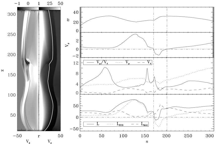
Figure 3: Snapshot of a two component jet simulation surrounded by an external medium of constant pressure. On the left panel, the toroidal velocity (left) and the corresponding poloidal velocity (right) are displayed. It also gives the cylindrical radius $\varpi(z)$ as a function of $z$. The reversal of the rotation corresponds to the darkest zone of the $V_{\varphi}$ contours. A specific streamline has been selected (solid line) along which the quantities shown on the right panel are plotted. From top to bottom: the cylindrical radius $\varpi(s)$ the angular momentum flux, the toroidal speed, the poloidal and Alfvén speeds, and the poloidal Alfvénic Mach number as functions of the curvilinear abscissa, $s$. The angular momentum flux (solid line) has two components, the hydrodynamical one ($L_{\rm HYDRO}$, dotted line) and the magnetic one ($L_{\rm MAG}$, dashed line).

During the initial transient phase, a strong shock propagates upwards due to the fact that the initial state is not in equilibrium. Together with the shock, a significant reversal of the toroidal velocity is also observed, although this phenomenon is not directly related with the above analysis. Once the system reaches a quasi-steady state, several layers demonstrate an opposite $V_{\varphi}$. These counter rotating regions remain roughly at the same location for large time intervals, before they vanish and reappear. They obviously remain transient phenomena.

The left panel of Fig. 3 displays contours of the toroidal velocity on the left and the poloidal component on the right. We have selected a streamline ($\varpi(z)$, grey and white solid lines of left panel) that crosses the region where the rotation reverses, along which the cylindrical radius, the angular momentum fluxes, the toroidal, poloidal and poloidal Alfvén speeds as well as the poloidal Alfvénic Mach number are shown on the right panel of Fig. 3.

The plots suggest that the $V_{\varphi}$ component becomes negative at the location where the poloidal velocity decreases approaching the Alfvén speed. Note that the flow remains always super-Alfvénic. The dotted dashed vertical lines indicate the change of sign of the rotation. In this region, the poloidal velocity reaches the local threshold value which varies along the flow. Although the jet is not an exact steady flow, the simulation results can be explained based on the analysis that describes the super Alfvénic regime.

On Fig. 3 we plot the total angular momentum flux $L$ and its two components (see Eq. 2), namely th hydrodynamical part $L_{\rm HYDRO}=\varpi V_{\varphi}$ and the magnetic one $L_{\rm MAG}=-\varpi\frac{B_{\rm p}}{4\pi\rho V_{\rm p}}B_{\varphi}$. The total angular momentum flux is clearly not conserved because the configuration is not in an exact steady state. However the reversal of the toroidal velocity corresponds to an exchange between the two components where the magnetic part becomes dominant. $L$ drops rapidly up to $s=190$. In this first part the reversal of the velocity is strongly time dependent and related to the shock as suggested by Fendt (2011). Above $s=190$, $L$ is almost constant and in this region our steady state criterion for the reversal is valid. It is a nice illustration of the above theory.

3 Conclusions

We have presented a simple study showing that counter rotation may occur in any jet or wind independently of the launching mechanism. Counter rotation may be observed in the outer layers of a disk wind, as shown in our numerical simulation and is observed in some protostellar jets. It may also occur in a stellar wind, as suggested from the data of the solar wind. This effect does not contradict the disk launching mechanism, nor the conservation of the angular momentum along the poloidal field lines. The criterion that marks the reversal of $V_{\varphi}$ is determined by either a deceleration of the flow or a specific geometrical configuration.

For the Sun, the toroidal velocity of the solar wind is very small or negative because there is almost no acceleration after the Alfvén point. In outflows associated with YSOs we expect that there may be reversals of the rotation in some of the layers of the flow but not necessarily across or along the whole jet. There is no evidence that this phenomenon should be permanent even if it is not a transient modification of the flow dynamics. In all cases, the total angular momentum is conserved, Eq. (2), although the kinetic and magnetic terms constituting $L(A)$ are expected to exchange the amount they store. The situation is similar to the transfer of energy from the enthalpy to the kinetic term in the Bernoulli integral in the thermally driven Parker wind, or, to the transfer of energy from the Poynting energy term at the base to the kinetic energy term at large distances in the generalized Bernoulli integral in magneto-centrifugal winds.

References

- Blandford & Payne (1982) Blandford, R. D., & Payne, D. G. 1982, MNRAS, 199, 883
- Cabrit et al. (2006) Cabrit S., Pety J., Pesenti N., Dougados C., 2006, A&A, 452, 897
- Coffey et al. (2004) Coffey D., Bacciotti F., Woitas J., Ray T. P., Eislöffel J., 2004, ApJ, 604, 758
- Coffey et al. (2011) Coffey D., Bacciotti F., Chrysostomou A., Nisini B., Davis C., 2011, A&A, 526, A40
- Coffey et al. (2012) Coffey D., Rigliaco E., Bacciotti F., Ray T. P., Eislöffel J., 2012, ApJ, 749, 139
- Fendt (2011) Fendt C., 2011, ApJ, 737, 43
- Heyvaerts & Norman (1989) Heyvaerts J., Norman C.A., 1989, ApJ, 347, 1055
- Lovelace, Berk, & Contopoulos (1991) Lovelace R. V. E., Berk H. L., Contopoulos J., 1991, ApJ, 379, 696
- Matsakos et al. (2012) Matsakos T., Vlahakis N., Tsinganos K. et al., 2012, A&A, in press
- Melnikov et al. (2009) Melnikov S. Y., Eislöffel J., Bacciotti F., Woitas J., Ray T. P., 2009, A&A, 506, 763
- Mignone et al. (2007) Mignone A., Bodo G., Massaglia S., Matsakos T., Tesileanu O., Zanni C., Ferrari A., 2007, ApJS, 170, 228
- Sauty et al. (2005) Sauty C., Lima J. J. G., Iro N., Tsinganos K., 2005, A&A, 432, 687
- Sauty et al. (2011) Sauty C., Meliani Z., Lima J. J. G., Tsinganos K., Cayatte V., Globus N., 2011, A&A, 533, A46
- Tsinganos (1982) Tsinganos K.C., 1982, ApJ, 252, 775
- Woitas et al. (2005) Woitas J., Bacciotti F., Ray T. P., Marconi A., Coffey D., Eislöffel J., 2005, A&A, 432, 149