Fractal dynamics in chaotic quantum transport

Abstract

Despite several experiments on chaotic quantum transport in two-dimensional systems such as semiconductor quantum dots, corresponding quantum simulations within a real-space model have been out of reach so far. Here we carry out quantum transport calculations in real space and real time for a two-dimensional stadium cavity that shows chaotic dynamics. By applying a large set of magnetic fields we obtain a complete picture of magnetoconductance that indicates fractal scaling. In the calculations of the fractality we use detrended fluctuation analysis – a widely used method in time series analysis – and show its usefulness in the interpretation of the conductance curves. Comparison with a standard method to extract the fractal dimension leads to consistent results that, in turn, qualitatively agree with the previous experimental data.

I Introduction

Since the pioneering works of Mandelbrot Mandelbrot (1983), fractal patterns have been found in a variety of objects in nature including, e.g., snowflakes, fern leaves, coastlines Mandelbrot (1967); Meakin (1998), and even music Voss:1975wm ; Hsu:1990wv ; Hennig:2011hq ; Hennig:2012vl . These self-similar (or self-affine) structures were also found in many branches of chemistry and physics; prominent examples are crystal growth and fractal surfaces, and transport in gold nanowires and electron “billiards” Meakin (1998); Michely and Krug (2004); Barnsley and Mathematics (2012); Sachrajda:1998wz ; adam98 ; Hegger et al. (1996); adam04 ; marlow ; adam12 . In contrast with idealized mathematical fractals continuing to infinitely small scales, fractal scaling in nature has a lower and an upper limit.

While fractals found in nature are often well described by classical theories Mandelbrot (1983); Meakin (1998); Michely and Krug (2004); Barnsley and Mathematics (2012), fractals have also been suggested to manifest in different quantum systems Berry (1996); Wójcik et al. (2000); Hufnagel et al. (2001); Benenti et al. (2001); Guarneri and Terraneo (2001); Louis:2000wg , where a fundamental lower cutoff for fractal scaling is given by the Heisenberg uncertainty principle. In the case of transport through chaotic systems, such as chaotic electron billiards, both semiclassical Ketzmerick (1996) (involving quantum interference) and classical mechanisms Hennig et al. (2007) for the emergence of fractal scaling have been proposed.

For quantum systems with an underlying classically mixed phase space with both regular and chaotic regions, a quantum graph model suggests a splitting of the chaotic regime into two parts Hufnagel et al. (2001): one part yields fractal conductance fluctuations while the other one leads to isolated resonances on small scales. These isolated resonances were later shown to be associated with the eigenstates of a closed system Bäcker et al. (2002).

A stadium quantum billiard of charged particles is a generic chaotic system, whose underlying classical phase space is chaotic. The phase space becomes mixed in presence of a (perpendicular) magnetic field. In the past two decades the system has been subject to several experiments Marcus:1992ug ; Micolich:2001vh ; Takagaki:2000ud ; Kuhl et al. (2005); Sachrajda:1998wz . A typical setup consists of the two-dimensional (2D) electron gas (2DEG) in a semiconductor heterostructure, where metallic gates are used to form the geometrical shape of the “billiards” – here called a quantum dot. Alternatively, stadium billiards (and other chaotic systems) can be realized experimentally with microwave cavities Kuhl et al. (2005).

Dynamics in chaotic cavities has been extensively studied with various theoretical methods including, e.g., random matrix theory  Baranger:1994 , trajectory-based semiclassical theory  Heusler:2006 , quantum mechanical kicked-rotor models Casati:2000 , and tight-binding calculations Louis:2000wg . Semiclassical and random matrix theory have been used to investigate weak localization and Ehrenfest time effects Jacquod:2006 ; Brouwer:2006 , while the kicked-rotor model and tight-binding studies have focused on the fractal structure of the quantum survival probability in chaotic cavities and the effect of changing the width of the output leads Louis:2000wg , respectively. Benenti et al. provide evidence for fractal fluctuations of the quantum survival probability in nonclassical situation of strong localization Benenti et al. (2001). However, to the best of our knowledge, none of the previous dynamical approaches have focused on conductance calculations in 2D chaotic cavities described by real-space grids in space and time.

It is worthwhile to notice that, in principle, the conductance problem of a chatic cavity can be treated within the conventional transport formalism, where the equilibrium current is obtained time-independently transport . In this approach, the coupling matrix of the cavity eigenstates and the lead states need to be evaluated. The most tedious part is an accurate and efficient treatment of the 2D eigenvalue problem for the chaotic cavity in real space and in the presence of the magnetic field. Recent progress has been made in this direction perttu , and such a conventional transport scheme is subject of future work. Nevertheless, as shown below, the present dynamical approach provides an efficient way to assess the conductivity and gives also additional information on time-dependent effects in the system.

In this work we calculate the fractal scaling of conductance fluctuations in an open quantum stadium billiard in a full 2D model in real space and real time. Our explicit solution of the time-dependent Schrödinger equation for chaotic transport goes beyond both the semiclassical treatment Ketzmerick (1996) and the above mentioned quantum graph model Hufnagel et al. (2001). We analyze the fractal scaling using two methods that originate from different fields of physics: the variation method Meakin (1998); Dubuc:1989vq ; Sachrajda:1998wz and detrended fluctuation analysis Peng et al. (1995); Kantelhardt:2001uk ; PengDNA (DFA). The variation method was used by Sachrajda et al. Sachrajda:1998wz for the analysis of experimental magnetoconductance curves. We are able to find a good agreement between theory and experiment, both yielding a fractal dimension $D\sim 1.3$.

II Model and the computational scheme

We consider a model for semiconductor stadium device fabricated in the 2DEG of a AlGaAs/GaAs heterostructure similar to Ref. Sachrajda:1998wz . The Hamiltonian describing our 2D system reads (in atomic units)

$$\hat{H}=\frac{1}{2}\left[-i\nabla+\mathbf{A}(\mathbf{r})\right]^{2}+V_{\rm ext}(\mathbf{r},t),$$ (1)

where the vector potential is given in the linear gauge, $\mathbf{A}(\mathbf{r})=(-By,0,0)$, to describe a static and uniform magnetic field perpendicular to the plane. During the time-propagation at $t>0$, the potential $V_{\rm ext}(\mathbf{r},t)$ consists of three parts: (i) a stadium with radius $r=1$ and width $d=0.7$, (ii) input and output leads of width $w=0.56$, and (iii) a linear potential along the propagation direction in the first two thirds of the input lead describing a source-drain voltage. The potential has hard boundaries with a depth $V_{0}=10000$ and the slope of the accelerating linear potential is $-100$. The central part of the external potential is shown in Fig. 1. The input and output lead extend further to the left and right.

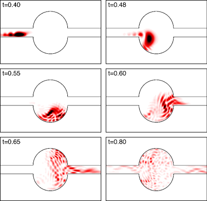
Figure 1: Snapshots of the electron density in the model stadium system (see text) during a transport simulation with the magnetic flux $\Phi/\Phi_{0}=20$. The input and output leads extend further to the left and right.

The initial state at $t=0$ is calculated by taking a small part of the input lead as a potential well. The resulting ground state of a single electron in the well is then used as an initial state for the time propagation. At $t>0$ the above described linear potential accelerates the wave packet across the system. For the time propagation we use a fourth-order Taylor expansion of the time-evolution operator. The octopus code package Octopus is used in all the calculations.

We assess the conductance by calculating the integrated probability density in the output lead from

$$T(\Phi,t)=\int_{\rm output}\mathrm{d}\mathbf{r}|\psi(\Phi,\mathbf{r},t)|^{2},$$ (2)

where $\Phi$ is the fixed magnetic flux, given above in units of the magnetic flux quantum $\Phi_{0}=h/e$. We call $T$ as a transmission factor assumed to be proportional to the transmission coefficient available in conventional transport theory. The validity of the transmission factor in estimating the relative conductivity as a function of an external parameter – here the magnetic flux – has been justified in Ref. rings . Thus, we repeat the time-propagation for different values of $\Phi$ to obtain the magnetoconductance that can be compared with the experiments in Ref. Sachrajda:1998wz .

It is important to note that our calculations allow energy dispersion for the wave functions in the cavity, i.e., we describe nonstationary states. In this respect, our results are not directly comparable to those of Ref. Ketzmerick (1996). However, our transport approach qualitatively describes an experimental situation to the extent that each value for the magnetic field is treated equally, so that we can compare the relative conductance as a function of $B$. Previously, a similar approach has been used to assess quantum conductance in quantum rings rings and Aharonov-Bohm interferometers ab1 .

III Transport simulations

In Fig. 1 we show snapshots of the electron density at different times at $\Phi=20\Phi_{0}$ through the stadium. Approximately one half of the density is transferred through and other half is either reflected back to the input lead or confined in the stadium. As expected, the density is scattered in the stadium in a chaotic fashion. The size of the wiggles during the scattering depends on the momentum – the higher the momentum the higher eigenstates are probed. We point out that the modes are not set prior to the calculation, but the wave packet is freely scattered and dispersed in the cavity. Here, we have chosen the initial momentum of the wave packet such that considerable overlap is found with $\sim 50\ldots 100$ eigenstates of the stadium during the transport. This corresponds to considerable qualitative complexity in the propagated density, which, as shown below, leads to a complex behavior of $T$. On the other hand, the momentum is limited by the grid spacing of the simulation box – all the nodes in the scattered wave packet should be accurately described.

A complete presentation of our transport results is given in Fig. 2, where the transmission factor $T$ is plotted as a function of both time and the magnetic flux. The figure consists of 401 respective time-propagations, each with a fixed number of flux quanta $\Phi/\Phi_{0}$ ranging from zero to 40 in steps of 0.1. The flux range is qualitatively similar to the experiment in Ref. Sachrajda:1998wz . A complex magnetoconductance is formed if the propagation time is larger than $\sim 1$. A cross section of the conductance at $t=1.4$ is shown in Fig. 3. We point out that due to the finite system size we are not able to reach the equilibrium current and thus find the absolute conductance. In practice, we stop the time-propagation immediately when the backscattering from the walls of the calculation box becomes visible. Therefore, we consider fixed propagation times through the parameter range of $\Phi/\Phi_{0}$. In other words, a fixed propagation time is expected to treat all the values of $\Phi/\Phi_{0}$ equally in order to obtain the relative conductance $T$.

We first briefly consider the general trends in $T$ in Fig. 3. As the flux is increased from zero the conductance decreases mainly due to the vanishment of trajectories directly coupling the left and the right lead. After reaching the minimum the conductance generally becomes larger, which is due to the increase of skipping orbits along the boundaries of the system. At large fields, interference effects play an important role vanhouten . We point out, however, that the dynamics is largely chaotic through the whole range of fluxes considered here – possibly only apart from the zero-flux limit.

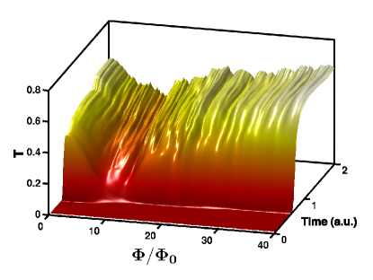
Figure 2: Transmission factor as a function of time and magnetic flux through the stadium.

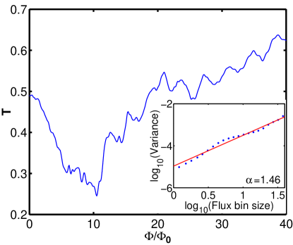
Figure 3: Transmission factor as a function of the magnetic flux at $t=1.4$. The inset shows the scaling exponent $\alpha=1.46$ obtained from the DFA analysis.

Now, the essential question is whether the conductance as a function of the magnetic flux shows fractal characteristics. Moreover, it is interesting to consider how large propagation times are required to find fractals. This is analyzed in the following with two techniques: the variation method Meakin (1998); Dubuc:1989vq ; Sachrajda:1998wz , and DFA Peng et al. (1995); Kantelhardt:2001uk ; PengDNA .

IV Methods for fractal analysis

IV.1 Variation method

To extract the fractal dimension $D$ for a mapping $f:\mathbb{R}\to\mathbb{R}$, the domain of the given function is first divided into length intervals $\Delta x$. The difference between the minimum and maximum of the function is calculated within every interval and added up. Note that the intervals are shifted window-wise accross the x-axis (not point-wise). In case of fractal scaling, the resulting sum is a power-law function of the interval length Meakin (1998); Dubuc:1989vq ; Sachrajda:1998wz :

$$\sum_{i}[\max f(x)-\min f(x)]_{|x-x_{i}|<\Delta x/2}\propto (\Delta x)^{-D+1}.$$ (3)

IV.2 Detrended fluctuation analysis

DFA is a standard method that was developed in the context of time-series analysis to study $1/f$ noise and long-range correlations Peng et al. (1995) and has proven to be very reliable particularly in dealing with non-stationary time-series and trends in the data Peng et al. (1995); Kantelhardt:2001uk ; Jennings:2004il ; Ivanov:2009ei ; Hennig:2011hq . It has also been used outside the time domain, e.g., to study the organization of DNA nucleotides PengDNA . However, to our knowledge, DFA has not been applied to fractal conductance curves before, and the application of DFA to reproducible fractals is typically not straightforward.

The standard procedure of DFA consists of the following four steps Peng et al. (1995); Kantelhardt:2001uk : (1) integrating the time series, (2) dividing the series into windows of size $s$, (3) fitting with a polynomial $f_{s}(i)$ of degree $m=2\ldots 4$ that represents the trend in the window, and (4) calculating the variance with respect to the local trend $f_{s}(i)$ from

$$F(s) = \left<(f(i)-f_{s}(i))^{2}\right>$$ (4)

$$= \frac{1}{N-1}\sum_{i=1}^{N}\left(f(i)-f_{s}(i)\right)^{2}\propto s^{\alpha}.$$

The key point in applying DFA to study conductance fluctuations is to relate the exponent $\alpha$ to the quantity of interest (here: the fractal dimension $D$). It is known that $D=2-\gamma/2$ with $\left<(\Delta G)^{2}\right>\propto(\Delta B)^{\gamma}$ Sachrajda:1998wz ; Ketzmerick (1996). The latter is exactly step (4) of the DFA analysis above. We therefore omit step (1) and identify $\alpha=\gamma$, hence the fractal dimension reads $D=2-\alpha/2$.

V Results on the fractality

In DFA, we apply quadratic detrending ($m=2$) to our data in Fig. 3. The inset shows the fitting of the data (solid line) at $t=1.4$ that yields $\alpha=1.46$. This qualitatively agrees well with the experimental result $\gamma=\alpha=1.38$ of Sachrajda et al. Sachrajda:1998wz . The corresponding fractal dimension extracted from DFA is $D=1.27$. In comparison, the variation method yields $D=1.32$ for our data, whereas the corresponding experimental result – obtained with the same method – is $D=1.25$ Sachrajda:1998wz . The expected error bars for our results are discussed below. Nevertheless, we find an excellent qualitative agreement of the results both regarding the different methods and comparison with the experimental data. We point out that our stadium model is similar to the experiment and the channel dimensions are also comparable. According to our calculations, increasing the channel width from $0.56$ to $0.7$ leads to the same $D$ obtained in the variation method, whereas DFA yields a slightly smaller $D$.

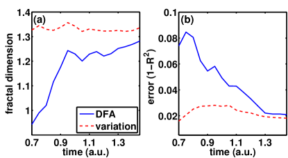
Figure 4: (a) Fractal dimension $D$ calculated from DFA with the relation $D=2-\alpha/2$ and from the variation method, respectively, during the time-propagation. Note that the fractal structure is developed only at $t\gtrsim 1$. (b) Time-development of the error in the fitting procedure at $t=0.7\ldots 1.4$ (see text).

In Fig. 4(a) we show the time-development of the fractal dimension obtained from DFA and the variation method, respectively. We point out that clear signatures of a fractal structure are developed only at $t\gtrsim 1$. Nevertheless, $D$ converges during the time-propagation towards the values given above, and the quality of the fitting in both methods improves as well. Figure 4(b) shows the error in the fitting, ${\rm ERR}=1-R^{2}$, for times $t=0.7\ldots 1.4$. Here $R$ is the Pearson product-moment correlation coefficient of the log-log data. Thus, ERR measures the linear fit quality such that ${\rm ERR}=0$ corresponds to exact linear behavior. The minimum of the error is obtained at $t\approx 1.4$, which is the optimal time used above to determine $\alpha$ and $D$. At larger times with $t\gtrsim 1.4$ the error increases due to back-scattering effects resulting from the finite simulation box (see above). In this way we are able to determine the range of validity in our scheme to calculate the fractal dimension.

It is important to note that in addition to the numerical error of the fitting procedure (see above), the algorithms for fractal analysis have internal error bars analyzed in detail by Pilgram and Kaplan Pilgram . For example, DFA results for the fractal scaling are expected to have a standard deviation of $\sim 15\%$ for data sets that are the of same size with ours. The results from the variational analysis are expected to contain similar deviations.

Finally we point out that qualitatively similar fractal dimensions have been obtained in various experiments on billiard systems of different shapes adam98 ; adam04 ; marlow . The dependence of $D$ on energy-level resolution determined by experimental conditions has been discussed in several works adamreview . Moreover, the considerable role of disorder in the modulation-doped 2DEG was recently demonstrated adam12 . However, in the same work it was shown that electrostatic doping leads to reproducible properties in thermal cycling. In view of these recent advances it can be expected that ballistic transport properties of 2DEG billiard systems will be determined in forthcoming experiments with a high precision. In turn, this motivates us to extend the applications of the present method to various geometries.

VI Summary

In summary, we have calculated the time-evolution of a single-electron wave packet through a two-dimensional stadium-shaped cavity by solving the Schrödinger equation in real time and real space. The relative conductance has been calculated for a large set of magnetic fluxes in order to analyze the fractal nature of the magnetoconductance. We have found that the conductance shows clear indications for fractal scaling. The fractal dimensions extracted from two respective methods are consistent with each other. Moreover, we have found an excellent qualitative agreement with previous experimental results. Our findings indicate that DFA suits well for the analysis of fractal scaling in chaotic quantum transport. Hence, we suggest to extend the use of the concept of data detrending (and hence DFA) to study fractal scaling of transport and other characteristics in chaotic (quantum) systems.

- (1)
- Mandelbrot (1983) B. B. Mandelbrot, The Fractal Geometry of Nature - Benoit B. Mandelbrot - Google Books (1983).
- Mandelbrot (1967) B. Mandelbrot, Science 156, 636 (1967).
- Meakin (1998) P. Meakin, Cambridge University Press (1998).
- (5) R. Voss and J. Clarke, Nature 258, 317 (1975).
- (6) K. J. Hsu and A. J. Hsu, Proc. Nat. Acad. Sci. 87, 938 (1990).
- (7) H. Hennig, R. Fleischmann, A. Fradebohm, Y. Hagmayer, J. Nagler, A. Witt, F. J. Theis, and T. Geisel, PLoS ONE 6, e26457 (2011).
- (8) H. Hennig, R. Fleischmann, and T. Geisel, Physics Today 65, 64 (2012).
- Michely and Krug (2004) T. Michely and J. Krug, Islands, Mounds, and Atoms, Patterns and Processes in Crystal Growth Far from Equilibrium (Springer Verlag, 2004).
- Barnsley and Mathematics (2012) M. F. Barnsley and Mathematics, Fractals Everywhere (2012).
- (11) A. S. Sachrajda, R. Ketzmerick, C. Gould, Y. Feng, P. J. Kelly, A. Delage, and Z. Wasilewski, Phys. Rev. Lett. 80, 1948 (1998).
- (12) A. P. Micolich, R. P. Taylor, R. Newbury, J. P. Bird, R. Wirtz, C. P. Dettmann, Y. Aoyagi, and T. Sugano, J. Phys.: Condens. Matter 10, 1339 (1998).
- Hegger et al. (1996) H. Hegger, B. Huckestein, K. Hecker, M. Janssen, A. Freimuth, G. Reckziegel, and R. Tuzinski, Phys. Rev. Lett. 77, 3885 (1996).
- (14) A. P. Micolich, R. P. Taylor, T. P. Martin, R. Newbury, T. M. Fromhold, A. G. Davies, H. Linke, W. R. Tribe, L. D. Macks, C. G. Smith, E. H. Linfield and D. A. Ritchie, Phys. Rev. B 70, 085302 (2004).
- (15) C. A. Marlow, R. P. Taylor, T. P. Martin, B. C. Scannell, H. Linke, M. S. Fairbanks, G. D. R. Hall, I. Shorubalko, L. Samuelson, T. M. Fromhold, C. V. Brown, B. Hackens, S. Faniel, C. Gustin, V. Bayot, X. Wallart, S. Bollaert, and A. Cappy, Phys. Rev. B 73, 195318 (2006).
- (16) A. M. See, I. Pilgrim, B. C. Scannell, R. D. Montgomery, O. Klochan, A. M. Burke, M. Aagesen, P. E. Lindelof, I. Farrer, D. A. Ritchie, R. P. Taylor, A. R. Hamilton, and A. P. Micolich, Phys. Rev. Lett. 108, 196807 (2012).
- Berry (1996) M. V. Berry, J. Phys. A 29, 6617 (1996).
- Wójcik et al. (2000) D. Wójcik, I. Białynicki-Birula, and K. Życzkowski, Phys. Rev. Lett. 85, 5022 (2000).
- Hufnagel et al. (2001) L. Hufnagel, R. Ketzmerick, and M. Weiss, Europhysics Letters 54, 703 (2001).
- Benenti et al. (2001) G. Benenti, G. Casati, I. Guarneri, and M. Terraneo, Phys. Rev. Lett. 87, 014101 (2001).
- Guarneri and Terraneo (2001) I. Guarneri and M. Terraneo, Phys. Rev. E 65, 015203 (2001).
- (22) E. Louis and J. A. Vergés, Phys. Rev. B 61, 13014 (2000)
- Ketzmerick (1996) R. Ketzmerick, Phys. Rev. B 54, 10841 (1996).
- Hennig et al. (2007) H. Hennig, R. Fleischmann, L. Hufnagel, and T. Geisel, Phys. Rev. E 76, 015202(R) (2007).
- Bäcker et al. (2002) A. Bäcker, A. Manze, B. Huckestein, and R. Ketzmerick, Phys. Rev. E 66, 016211 (2002).
- (26) C. M. Marcus, A. J. Rimberg, R. M. Westervelt, P. F. Hopkins, and A. C. Gossard, Phys. Rev. Lett. 69, 506 (1992).
- (27) A. P. Micolich, R. P. Taylor, A. G. Davies, J. P. Bird, R. Newbury, T. M. Fromhold, A. Ehlert, H. Linke, L. D. Macks, W. R. Tribe, E. H. Linfield, D. A. Ritchie, J. Cooper, Y. Aoyagi, and P. B. Wilkinson Phys. Rev. Lett. 87, 036802 (2001).
- (28) Y. Takagaki, M. ElHassan, A. Shailos, C. Prasad, J. P. Bird, D. K. Ferry, K. H. Ploog, L.-H. Lin, N. Aoki, and Y. Ochiai, Phys. Rev. B 62, 10255 (2000).
- Kuhl et al. (2005) U. Kuhl, H.-J. Stöckmann, and R. Weaver, J. Phys. A 38, 10433 (2005).
- (30) H. U. Baranger and P. A. Mello, Phys. Rev. Lett. 73, 142 (1994).
- (31) S. Heusler, S. Müller, P. Braun, and F. Haake, Phys. Rev. Lett. 96, 066804 (2006).
- (32) G. Casati, I. Guarneri, and G. Maspero, Phys. Rev. Lett. 84, 63 (2000).
- (33) Ph. Jacquod and R. S. Whitney, Phys. Rev. B 73, 195115 (2006).
- (34) P. W. Brouwer and S. Rahav, Phys. Rev. B 74, 075322 (2006).
- (35) For recent reviews on quantum transport, see, e.g., M. Di Ventra, Electrical Transport in Nanoscale Systems (Cambridge University Press, 2008); G. Stefanucci and R. van Leeuwen, Nonequilibrium Many-Body Theory of Quantum Systems: A Modern Introduction (Cambridge University Press, 2013).
- (36) P. J. J. Luukko and E. Räsänen, Comp. Phys. Comm. 184, 769 (2013).
- (37) B. Dubuc, J. F. Quiniou, C. Roques-Carmes, C. Tricot, and S. W. Zucker, Phys. Rev. A 39, 1500 (1989).
- Peng et al. (1995) C. K. Peng, S. Havlin, H. E. Stanley, and A. L. Goldberger, Chaos 5, 82 (1995).
- (39) J. W. Kantelhardt, E. Koscielny-Bunde, H. H. A. Rego, S. Havlin, and A. Bunde, Physica A 295, 441 (2001).
- (40) C.-K. Peng, S. V. Buldyrev, S. Havlin, M. Simons, H. E. Stanley, and A. L. Goldberger, Phys. Rev. E 49, 1685 (1994).
- (41) M. A. L. Marques, A. Castro, G. F. Bertsch, A. Rubio, Comput. Phys. Commun. 151, 60 (2003); A. Castro, H. Appel, M. Oliveira, C. A. Rozzi, X. Andrade, F. Lorenzen, M. A. L. Marques, E. K. U. Gross, and A. Rubio, Phys. Stat. Sol. (b) 243, 2465 (2006).
- (42) V. Kotimäki and E. Räsänen, Phys. Rev. B 81, 245316 (2010).
- (43) V. Kotimäki, E. Cicek, A. Siddiki, and E. Räsänen, New J. Phys. 14, 053024 (2012).
- (44) H. van Houten, C. W. J. Beenakker, J. G. Williamson, M. E. I. Broekaart, and P. H. M. van Loosdrecht, B. J. van Wees, J. E. Mooij, C. T. Foxon, and J. J. Harris, Phys. Rev. B 39, 8556 (1989).
- (45) H. D. Jennings, P. C. Ivanov, A. M. Martins, P. C. Silva, and G. M. Viswanathan, Physica A 336, 585 (2004).
- (46) Plamen Ch. Ivanov, Qianli D. Y. Ma, Ronny P. Bartsch, Jeffrey M. Hausdorff, Luís A. Nunes Amaral, Verena Schulte-Frohlinde, H. E. Stanley, and Mitsuru Yoneyama, Phys. Rev. E 79, 041920 (2009).
- (47) B. Pilgram and D. T. Kaplan, Physica D 114, 108 (1997).
- (48) For a review, see A. P. Micolich, A. M. See, B. C. Scannell, C. A. Marlow, T. P. Martin, I. Pilgrim, A. R. Hamilton, H. Linke, and R. P. Taylor, Fortschr. Phys. 60, 1 (2012).