Why does the Jeans Swindle work?

Abstract

When measuring the mass profile of any given cosmological structure through internal kinematics, the distant background density is always ignored. This trick is often refereed to as the “Jeans Swindle”. Without this trick a divergent term from the background density renders the mass profile undefined, however, this trick has no formal justification. We show that when one includes the expansion of the Universe in the Jeans equation, a term appears which exactly cancels the divergent term from the background. We thereby establish a formal justification for using the Jeans Swindle.

1 Introduction

A small overdensity in an otherwise infinite homogeneous gravitating system (like any cosmological structure in the Universe) is affected by a basic inconsistency, namely that such a system cannot be in equilibrium, and at the same time obey the Poisson’s equation which relates the gravitational potential to the density distribution. A constant gravitational potential leads, via Poisson’s equation, to a zero density (Jeans, 1929; Zeldovich & Novikov, 1971). The usual way to overcome this inconsistency is to assume that the infinite homogeneous system does not contribute to the gravitational potential, meaning that the gravitational potential is sourced only by fluctuations to this uniform background density. This assumption is called Jeans Swindle (Binney & Tremaine, 1987, 2008; Kiessling, 2003; Joyce, 2008; Ershkovich, 2011). Following Binney & Tremaine (1987) “it is a swindle because in general there is no formal justification for discarding the unperturbed gravitational field”. It is vindicated by the right results it provides, but it is generally considered a limitation to the formalism.

The Jeans Swindle has several applications. Here we focus on the Jeans Swindle in the context of the Jeans analysis of internal kinematics, which for instance is relevant for stellar motions in dwarf galaxies and galaxy motions in galaxy clusters. The aim of this work is to explain the “swindle” through a clean derivation of the Jeans equation, including the crucial expansion of the Universe.

The Jeans equation describes systems in equilibrium, and it is therefore used to model for example dark matter halos inside the virial region, where they can be treated as equilibrated systems. Dark matter (DM) halos can be seen as a matter excesses over the mean matter density of the Universe. This constant background density is the main contribution to the density distribution at large distances from the halo center (Tavio et al., 2008). We show that the contributions from the background density, the cosmological constant and the Hubble expansion, cancel each other. When omitting the constant background density (the normal “swindle”) one is actually excluding it together with the contribution from the expansion of the Universe. Thus, once we take into account the expansion of the Universe and the presence of the cosmological constant, we no longer need to invoke the Jeans Swindle.

2 Jeans Swindle in the Jeans equation

The dynamics of DM halos, modelled as spherical and stationary systems of collisionless particles in equilibrium, is controlled by the spherical non-streaming Jeans equation (Binney, 1980)

$$-\rho(r)\frac{\rm d\Phi}{\rm dr}=\frac{\rm d(\rho\sigma_{\rm r}^{2})}{\rm d\,r}+2\,\frac{\beta}{r}\rho\sigma_{\rm r}^{2}\,,$$ (1)

where $\sigma_{\rm r}$ is the radial velocity dispersion, $\beta=1-\sigma_{\theta}^{2}/\sigma_{\rm r}^{2}$ the velocity anisotropy, $\rho$ the density distribution of particles and $\Phi$ the total gravitational potential.

The potential gradient is given by Poisson’s equation

$$\frac{\rm d\Phi}{\rm dr}=\frac{GM(r)}{r^{2}}\,.$$ (2)

In the simple case of an isotropic velocity distribution ($\beta=0$), the solution to the standard Jeans equation (1) for the radial velocity dispersion is (from Binney, 1980)

$$\sigma_{\rm r}^{2}(r)=\frac{1}{\rho(r)}\int_{r}^{\infty}\rho(s)\,\left[\frac{GM(s)}{s^{2}}\right]\rm ds\,.$$ (3)

Thus, the only quantity required for the calculation of the radial dispersion is the density distribution of the halo. DM-only cosmological N-body simulations indicate that a double slope profile provides a reasonable fit to the density profiles of halos within the virial radius (Navarro et al., 1996; Kravtsov et al., 1998). Since the integration in equation (3) extends all the way to infinity, we need a correct description of the DM distribution beyond the virial radius. The correct asymptotic value should be the mean matter density of the Universe $\rho_{\rm bg}$, given by

$$\rho_{\rm bg}=\Omega_{M}\rho_{c}=\frac{3\,\Omega_{M}\,H^{2}}{8\pi\,G},$$ (4)

where $\Omega_{M}$ the matter density parameter, $\rho_{c}$ is the critical density of the Universe and $H=\dot{a}/a$ is the Hubble constant ($a$ being the scale factor of the Universe).

Therefore, the double slope profile, reaching zero density at large distances from the cluster center, does not reproduce the right density profile in the external region (Tavio et al., 2008). As a first approximation, we can write the density as given by the sum of a term $\rho_{\rm h}$ that reproduces the inner part of the halo distribution and the constant background density that affects the profile only at large radii

$$\rho(r)=\rho_{\rm h}(r)+\rho_{\rm bg}\,.$$ (5)

As an example, we consider a finite mass density profile for a cluster-size halo, the Hernquist (1990) profile 

$$\rho_{\rm h}(r)=\frac{\rho_{0}}{r/r_{\rm v}\,(1+r/r_{\rm v})^{3}}\,,$$ (6)

where $r_{\rm v}$ is the virial radius and $\rho_{0}$ is the characteristic density, that can be written in terms of the virial overdensity $\Delta$ as

$$\rho_{0}=\alpha\,\Delta\rho_{c}\,.$$ (7)

In Figure 1, we show the profile given by eq. (6) (black solid line) and the sum $\rho_{\rm h}(r)+\rho_{\rm bg}$ (green dash-dot line), where the asymptotic value is $\rho_{\rm bg}$ (red dashed line). In the calculation, we set $\Omega_{M}=0.24$, $\Delta=100$, $H=73\,\rm km\,s^{-1}\,Mpc^{-1}$ and we fix $\alpha$ by imposing that the mass given by the density in eq. (6) within the sphere of radius $r_{\rm v}$ corresponds to the virial mass

$$M_{\rm v}=\frac{4\pi}{3}r_{\rm v}^{3}\Delta\rho_{c}\,.$$ (8)

In Figure 1, the density is in units of $\Delta\rho_{c}$ and the radius is in units of the virial radius.

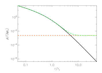
Figure 1: Black solid line: Hernquist profile given by equation (6). Red dashed line: background density given by equation (4). Green dash-dot line: the sum of the Hernquist profile and the constant background density.

Once we insert the expression (5) in the integral (3) we get

$$\sigma_{\rm r}^{2}(r) \!\!=\!\! \frac{1}{\rho_{\rm h}(r)\!+\!\rho_{\rm bg}}$$ (9)

$$\times\,\int_{r}^{\infty}\!\!G\,\left[\rho_{\rm h}(s)\!+\!\rho_{\rm bg}\right]\left[M_{\rm h}(s)\!+\!M_{\rm bg}(s)\right]\frac{\rm ds}{s^{2}}\,,$$

which diverges, since the background mass diverges at large radii. In Fig. 2 we plot the solution (9) for different upper limits $r_{\rm max}$ in the integral: $r_{\rm max}=200\,r_{\rm v}$ (blue short-dashed line), $r_{\rm max}=500\,r_{\rm v}$ (green dash-dot line), $r_{\rm max}=1000\,r_{\rm v}$ (magenta dash-dot-dot line).

This clearly indicates that when integrating to infinity, the integral will diverge.

The usual trick to avoid the divergence is to omit the contribution of the background density to the potential gradient (2), i.e. to set $\nabla\Phi_{\rm bg}=0$ (Binney & Tremaine, 1987, 2008; Ershkovich, 2011). Physically, this amounts to assume that the gravitational potential is sourced only by fluctuations to the uniform background density. For this requirement to be consistent with the Poisson’s equation (2), the constant $\rho_{\rm bg}$ in equation (5) has to vanish. This assumption is called the Jeans Swindle. It has no justification other than to overcome a mathematical difficulty.

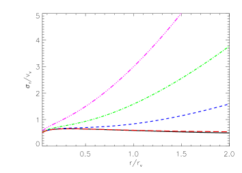
Figure 2: Radial velocity dispersion profiles. The black solid line corresponds to the standard Jeans solution (10). Solutions of equation (9) corresponding to different upper limits $r_{\rm max}$ in the integral are shown: $r_{\rm max}=200\,r_{v}$ (blue short-dashed line), $r_{\rm max}=500\,r_{v}$ (green dash-dot line), $r_{\rm max}=1000\,r_{v}$ (magenta dash-dot-dot line). The red long-dashed line is the solution when including cosmological expansion and background density (eq. [20]). The radial velocity dispersion is in units of the virial velocity and the radius is in units of the virial radius.

The Jeans analysis has always been performed by discarding the unperturbed density, so that equation (3) is just

$$\sigma_{\rm r}^{2}(r)=\frac{1}{\rho_{\rm h}(r)}\int_{r}^{\infty}\rho_{\rm h}(s)\left[\frac{G\,M_{\rm h}(s)}{s^{2}}\right]\rm ds\,.$$ (10)

The black solid line in fig. 2 corresponds to the computation of equation (10), which is not divergent.

With this approach, the Jeans equation reproduces the radial dispersion of DM halos from cosmological simulations in the region of equilibrium (Sanchis et al., 2004; Wojtak et al., 2005; Cuesta et al., 2008), and gives finite masses for dwarf galaxies (Strigari et al., 2010; Salucci et al., 2012).

3 Why the Jeans Swindle works

We wish to replace the Jeans Swindle by a formally correct analysis. Thus, we keep the background density $\rho_{\rm bg}$ and its contribution in the gravitational potential. The gradient of the potential due to $\rho_{\rm bg}$ can be put in the following form:

$$\frac{\rm d\Phi_{\rm bg}}{\rm dr}=\frac{4}{3}\pi\,G\rho_{\rm bg}\,r={\Omega_{\rm m}\over 2}\,H^{2}r\,,$$ (11)

where we have used equation (4). However, in order to be consistent, we need to take into account all effects due to the underlying cosmology. For the case of a single halo embedded in a homogeneous Universe with a non-zero cosmological constant $\Lambda$, particles also feel a repulsive potential of the form (e.g. Peirani & de Freitas Pacheco, 2006; Nandra et al., 2012)

$$\frac{\rm d\Phi_{\rm\Lambda}}{\rm dr}=-\frac{1}{3}\Lambda\,r=-\Omega_{\Lambda}\,H^{2}\,r\,,$$ (12)

where we have used the relation

$$\Omega_{\Lambda}=\frac{\Lambda}{3\,H^{2}}\,.$$ (13)

Introducing the deceleration parameter

$$q=-{\ddot{a}a\over\dot{a}^{2}}={\Omega_{\rm m}\over 2}-\Omega_{\Lambda},$$ (14)

we can rewrite the total contribution of the cosmology to the gravitational potential gradient as

$$\frac{\rm d\Phi_{\rm bg}}{\rm dr}+\frac{\rm d\Phi_{\Lambda}}{\rm dr}=q\,H^{2}\,r.$$ (15)

Moreover, the Universe is not static, but it is subject to the Hubble expansion. Equation (1) holds for structures that have achieved dynamical equilibrium. This means that the radial, longitudinal and azimuthal bulk motions are not taken into account in its derivation. When excluding all these bulk velocity terms, the Hubble flow, which DM particles are subject to, is also discarded. The Hubble velocity, $v_{H}=H\,r$, might be neglected in the very inner region, but for large radii, it becomes important. Since the integration in equation (3) extends to infinity, the inclusion of $v_{H}$ will affect the result.

When we include the terms involving the mean radial velocity, the Jeans equation becomes the more general formula (Falco et al., 2013)

$$-\rho\frac{\rm d\Phi}{\rm dr}=\frac{\rm d(\rho\sigma_{\rm r}^{2})}{\rm dr}+2\,\frac{\beta}{r}\rho\sigma_{\rm r}^{2}+\rho\left[\overline{v}_{\rm r}\frac{\partial\overline{v}_{\rm r}}{\partial r}+\frac{\partial\overline{v}_{\rm r}}{\partial t}\right]\,.$$ (16)

In the most general case, $v_{\rm r}$ is the sum of the Hubble velocity and a peculiar infall velocity. The infall velocity occurs around cluster-sized haloes ($M_{\rm vir}\approx\,10^{13-14}M_{\odot}$), and is totally negligible around galactic haloes ($M_{\rm vir}\approx\,10^{12}M_{\odot}$) (Prada et al., 2006; Cuesta et al., 2008). Streaming motions around clusters are dominated by the infall velocity at radii between the virial radius and the turn-around radius, which is approximately equal to $3.6$ virial radii (Cupani et al., 2008). At larger distances, it approaches the Hubble flow. Therefore, far outside the equilibrated cluster, we can neglect the mean radial peculiar motion of particles, so that the radial velocity corresponds to $v_{H}$ only

$$\overline{v}_{\rm r}(r,t)=H(t)\,r\,.$$ (17)

It is straightforward to calculate the additional term in square brackets in eq. (16)

$$\overline{v}_{\rm r}\frac{\partial\overline{v}_{\rm r}}{\partial r}+\frac{\partial\overline{v}_{\rm r}}{\partial t}=H^{2}\,r+\dot{H}\,r=-q\,H^{2}r\,,$$ (18)

where we used

$$\dot{H}=-(q+1)\,H^{2}\,.$$ (19)

We can now write equation (3) for large radii, including all these cosmological terms

$$\sigma_{\rm r}^{2}(r)\!\!\! \!\!\!=\!\!\! \!\!\!\frac{1}{\rho_{\rm h}(r)\!+\!\rho_{\rm bg}}\int_{r}^{\infty}\left[\rho_{\rm h}(s)\!+\!\rho_{\rm bg}\right]$$ (20)

$$\times\,\left[\frac{\rm d\Phi_{\rm h}}{\rm ds}\!+\!\frac{\rm d\Phi_{\rm bg}}{\rm ds}\!+\!\frac{\rm d\Phi_{\Lambda}}{\rm ds}\!+\!\overline{v}_{r}\frac{\partial\overline{v}_{r}}{\partial s}\!+\!\frac{\partial\overline{v}_{r}}{\partial t}\right]\rm ds$$

$$\!\!\!=\!\!\! \!\!\!\frac{1}{\rho_{\rm h}(r)\!+\!\rho_{\rm bg}}\int_{r}^{\infty}\left[\rho_{\rm h}(s)\!+\!\rho_{\rm bg}\right]$$

$$\times\,\left[\frac{GM_{\rm h}(s)}{s^{2}}\!+\!q\,H^{2}\,s|_{\rm bg,\Lambda}-q\,H^{2}\,s|_{H}\right]\rm ds$$

$$\!\!\!=\!\!\! \!\!\!\frac{1}{\rho_{\rm h}(r)\!+\!\rho_{\rm bg}}\int_{r}^{\infty}(\rho_{\rm h}(s)\!+\!\rho_{\rm bg})\,\left[\frac{GM_{\rm h}(s)}{s^{2}}\right]\rm ds\,.$$

We thus see that the term $-q\,H^{2}\,s|_{H}$ given by the Hubble velocity (18) cancels exactly the term $q\,H^{2}\,s|_{{\rm bg},\Lambda}$ given by the potentials of the background density and the cosmological constant. In this way, we recover the same result as applying the Jeans Swindle, and in the Jeans solution the total mass is again $M(s)=M_{\rm h}(s)$.

Formally, there is still a minor difference between the two approaches: the density involved in eq. (20) is still given by $\rho_{\rm h}(s)+\rho_{\rm bg}$, where $\rho_{\rm bg}$ is not zero but instead given by eq. (4). However, this time it does not lead to any divergence, because $M_{\rm h}(s)/s^{2}$ falls rapidly to zero at large distances. This can be seen in Figure 2, where the solution of eq. (20) is the red long-dashed line and it matches the result we obtain from equation (10)(black solid line). For larger radii, the addition of the background density in the density profile can affect the result slightly. However, in the outer regions, where the halos are no longer equilibrated, the standard Jeans equation is anyway not used to reproduce the radial velocity dispersion. Instead, the generalized Jeans equation in eq. (16) must be used, including the infall motion of galaxies. The addition of the peculiar velocity changes the shape of the velocity dispersion in the infall region (Falco et al., 2013), but it does not affect the conclusion of this work. One could also improve on this minor difference, by not including $\rho_{\rm bg}$ at all radii, but instead a different form which takes into account that the immediate environment of haloes may not be the cosmological value yet. A more accurate density profile would include a term to describe the local region around clusters, before the cosmological background is reached. For example, Cooray & Sheth (2002) give a detailed description of the halo model, where the background contribution to the total density is given by a more complicated function than the constant value $\rho_{\rm bg}$ only. This is equivalent to define $\rho_{\rm h}$ as

$$\rho_{\rm h}=\rho_{\rm tot}-\rho_{\rm bg}\,,$$ (21)

i.e. including in $\rho_{\rm h}$ the details of the background density being different from $\rho_{\rm bg}$. The equation (20) is formally not affected by this modification.

4 Comoving coordinates

The equations describing the particle distribution and motion can be written in comoving coordinates (Peebles, 1980). The physical coordinates $r$ and comoving coordinates $x$ are related by the universal time-dependent expansion parameter $a(t)$

$$r=a(t)\,x\,.$$ (22)

When changing variables from the physical space to the comoving one, the Poisson’s equation becomes (Peebles, 1980)

$$\nabla^{2}\phi=4\pi\,G\,a^{2}[\rho(x)-\rho_{\rm bg}]\,,$$ (23)

where the gradient is with respect to $x$, and $\rho_{\rm bg}$ is the mean mass density and $\phi(x)$ is the potential contributed by the overdensity $\rho-\rho_{\rm bg}$. Therefore, in this coordinate system, the particle motion is already described in terms of the departure from the constant background, and the swindle is not required. As we expect, taking into account the cosmological expansion in the physical space leads to the same result as moving to the expanding space. Equation (1) would be correct if we replaced $r$ with $x$ and $\Phi$ with $\phi$, and using $\rho$ given by (5), namely it is the correct Jeans equation in comoving coordinates.

Joyce & Sylos Labini (2012) have also shown that a cosmological N-body simulation of an isolated overdensity should reproduce, in physical coordinates, the same result as a simulation obtained for the structure in open boundary condition without expansion.

We conclude that our work is consistent with the comoving frame analysis by Peebles (1980) and with the conclusions of Joyce & Sylos Labini (2012) . This confirms that the Jeans Swindle corresponds to accounting for the expansion of the Universe.

5 Conclusions

We have demonstrated that the Jeans Swindle is not an ad hoc trick, but it is the result of correctly combining the mean matter density and the expansion of the Universe. The divergent term from the background density, which in a static universe would lead to a divergent dispersion profile, is exactly cancelled by a term from the expanding universe. We have shown that the dispersion profile measured when assuming no background and a static universe, is the same as the dispersion profile when including both the background density and the expansion. This means that we have establish a formal justification for using the Jeans Swindle. This result holds for radii smaller than roughly the virial radius. For larger radii one has to include the effect of infalling matter, which is done through a generalized Jeans equation, as will be presented in a forthcoming article (Falco et al., 2013).

References

- Binney (1980) Binney J., 1980, MNRAS, 190, 873
- Binney & Tremaine (1987) Binney J., Tremaine S., 1987, Galactic dynamics. Princeton University Press, pp. 287–296,681–686
- Binney & Tremaine (2008) Binney J., Tremaine S., 2008, Galactic Dynamics. Princeton University Press, pp. 401–403
- Cooray & Sheth (2002) Cooray A., Sheth R., 2002, Physics Reports, 372, 1
- Cuesta et al. (2008) Cuesta A. J., Prada F., Klypin A., Moles M., 2008, MNRAS, 389, 385
- Cupani et al. (2008) Cupani G., Mezzetti M., Mardirossian F., 2008, MNRAS, 390, 645
- Ershkovich (2011) Ershkovich A. I., 2011, ArXiv e-prints, arXiv:astro-ph/1108.5519
- Falco et al. (2013) Falco M., Mamon G. A., Wojtak R., Hansen S. H., Gottlöber S., 2013, to be submitted
- Hernquist (1990) Hernquist L., 1990, ApJ, 356
- Jeans (1929) Jeans J. H., 1929, The Universe Around Us. Cambridge, University Press
- Joyce (2008) Joyce M., 2008, American Institute of Physics Conference Series, 970, 237