Global Properties of M31’s Stellar Halo from the SPLASH Survey. I. Surface Brightness Profile

Abstract

We present the surface brightness profile of M31’s stellar halo out to a projected radius of 175 kpc. The surface brightness estimates are based on confirmed samples of M31 red giant branch stars derived from Keck/DEIMOS spectroscopic observations. A set of empirical spectroscopic and photometric M31 membership diagnostics is used to identify and reject foreground and background contaminants. This enables us to trace the stellar halo of M31 to larger projected distances and fainter surface brightnesses than previous photometric studies. The surface brightness profile of M31’s halo follows a power-law with index $-2.2\pm 0.2$ and extends to a projected distance of at least $\sim 175$ kpc ($\sim 2/3$ of M31’s virial radius), with no evidence of a downward break at large radii. The best-fit elliptical isophotes have $b/a=0.94$ with the major axis of the halo aligned along the minor axis of M31’s disk, consistent with a prolate halo, although the data are also consistent with M31’s halo having spherical symmetry. The fact that tidal debris features are kinematically cold is used to identify substructure in the spectroscopic fields out to projected radii of 90 kpc, and investigate the effect of this substructure on the surface brightness profile. The scatter in the surface brightness profile is reduced when kinematically identified tidal debris features in M31 are statistically subtracted; the remaining profile indicates that a comparatively diffuse stellar component to M31’s stellar halo exists to large distances. Beyond 90 kpc, kinematically cold tidal debris features can not be identified due to small number statistics; nevertheless, the significant field-to-field variation in surface brightness beyond 90 kpc suggests that the outermost region of M31’s halo is also comprised to a significant degree of stars stripped from accreted objects.

1. Introduction

Stellar halos of galaxies are low density environments in which the detritus of hierarchical structure formation can remain visible for Gigayears in the form of tidal debris structures. Detailed simulations of stellar halo formation in a cosmological context (Bullock et al., 2001; Bullock & Johnston, 2005; Font et al., 2006, 2008; Johnston et al., 2008; Zolotov et al., 2009, 2010; Cooper et al., 2010; Font et al., 2011) are providing a growing framework for interpreting observations of tidal debris in stellar halos. Current simulations suggest that galaxy mergers play a primary role in the formation of stellar halos: the outer regions of stellar halos are built via the accretion of smaller galaxies and tidal stripping of their stars, while the inner regions may be built through a combination of merging events and in situ star formation (Zolotov et al., 2010; Font et al., 2011; McCarthy et al., 2012). Thus, the global properties of stellar halos are a product of the merging history of the host galaxy.

Recent observational campaigns have extended studies of stellar halos beyond the Local Group (Tanaka et al., 2011; Martínez-Delgado et al., 2010; Radburn-Smith et al., 2011). However, M31 remains one of the best laboratories for studying stellar halos. M31’s proximity enables us to study its resolved stellar population not just with photometry, but also through spectroscopy of individual stars.

Early work on the integrated light of M31 (de Vaucouleurs, 1958; Walterbos & Kennicutt, 1987) was followed by resolved stellar population studies over the last several decades (e.g., Mould & Kristian, 1986; Ferguson et al., 2002). These studies found that within $R\sim 30$ kpc, the M31 stellar halo appeared to be a continuation of M31’s inner bulge, and was characterized by the following properties: a de Vaucouleurs $r^{1/4}$ law radial surface brightness profile (Pritchet & van den Bergh, 1994), a high stellar density (Reitzel et al., 1998), and a high mean metallicity ($\rm{[Fe/H]}\sim-0.5$ Mould & Kristian, 1986; Rich et al., 1996; Durrell et al., 2001; Reitzel & Guhathakurta, 2002; Bellazzini et al., 2003; Durrell et al., 2004). Furthermore, deep imaging (obtained with the Advanced Camera for Surveys on the Hubble Space Telescope) along M31’s minor axis at radii of 10 – 35 kpc (well beyond the extent of M31’s disk) revealed a significant population of $\sim 6$ – 8 Gyr stars (Brown et al., 2003, 2006, 2007, 2008). The properties of the inner regions of M31’s spheroid stand in stark contrast to the properties of the Milky Way’s (MW) stellar halo, which consists almost entirely of old, metal-poor stars and appears to follow a power-law density profile ($\rho(r)\propto r^{\gamma}$) . Studies of the MW’s halo have typically measured $\gamma\sim-2.7$ to $-3.5$ (e.g., Morrison et al., 2000; Yanny et al., 2000; Siegel et al., 2002; Jurić et al., 2008; Sesar et al., 2011), equivalent to a surface density distribution with a slope of -1.7 to -2.5.

In the past five years, large photometric and spectroscopic surveys have discovered and begun to characterize M31’s outer stellar halo, which has a power-law surface brightness profile, low stellar density, and metal-poor stars. Using the spectroscopic data set of Gilbert et al. (2006), Guhathakurta et al. (2005) showed that beyond projected radial distances of $R_{\rm proj}$ $\sim 20$ – 30 kpc, the surface brightness profile of M31’s stellar halo is consistent with a power-law of index $-2.3$ out to the limits of the surveyed region, $R_{\rm proj}$ $\sim 165$ kpc. A concurrent photometric study based on data from the Isaac Newton Telescope Wide-Field Camera (Irwin et al., 2005) also found evidence for a break in the radial surface brightness profile of M31 at $R_{\rm proj}$ $\sim 20$ kpc, and determined that beyond this radius the profile flattens and is consistent with a power-law index of $-2.3$; their study reached to a projected radial distance of 55 kpc from the center of M31. Ibata et al. (2007) presented a large photometric survey of M31’s southern quadrant undertaken with the Canada–France–Hawaii Telescope/MegaCam and found that the radial surface brightness profile of M31 out to $R_{\rm proj}$ $\sim 130$ kpc is consistent with a power-law of index $-1.9$.

M31’s outer stellar halo consists of stars that are on average more metal-poor than the stars that comprise the inner, bulge-like spheroid. Kalirai et al. (2006a) used the data set from Gilbert et al. (2006) to analyze the metallicity of red giant branch (RGB) stars from $R_{\rm proj}$ $\sim 11$ to 165 kpc in M31’s southern quadrant. They found that while the inner regions of M31’s spheroid are relatively metal-rich, the stellar population becomes increasingly metal-poor beyond $R_{\rm proj}$ $\sim 30$ kpc (see also Koch et al., 2008; Tanaka et al., 2010). A contemporaneous study found evidence of metal-poor M31 RGB stars from $R_{\rm proj}$ $\sim 10$ to 70 kpc in fields located near M31’s major axis (Chapman et al., 2006).

Most previous studies of M31’s stellar halo consisted primarily of fields in the southern quadrant of M31 or along M31’s southern minor axis. Two recent photometric surveys have extended observations of M31’s stellar halo into the other three quadrants, providing a more global view of the halo. The Pan-Andromeda Archaeological Survey (PAndAS; McConnachie et al., 2009) used the Canada–France–Hawaii Telescope (CFHT) and the MegaCam instrument to survey the eastern, northern, and western quadrants of M31’s halo out to a maximum projected radial distance of $\sim 150$ kpc. PAndAs found stellar sources consistent in color and apparent magnitude with RGB stars at the distance of M31 throughout the survey volume (McConnachie et al., 2009). Tanaka et al. (2010) surveyed along M31’s minor axis with the Suprime-Cam instrument on the Subaru Telescope, achieving a deeper photometric limit than PAndAS, although over a much more limited area. They observed strips of contiguous fields on the southeast and northwest minor axis out to projected distances of $R_{\rm proj}$ $\sim 60$ and $\sim 100$ kpc, respectively, and found the radial surface brightness profile along M31’s northwest minor axis is described by a power-law with an index of $-2.2$, consistent with results from the southeast minor axis.

Interpretation of the global properties of M31’s stellar halo is complicated by the presence of large, extended, and numerous tidal debris features (e.g., Ibata et al., 2001; Ferguson et al., 2002; Kalirai et al., 2006b; Ibata et al., 2007; Gilbert et al., 2007, 2009; McConnachie et al., 2009; Tanaka et al., 2010). It is difficult to assess the effect of substructure on measured values (mean metallicity, surface brightness profile) with purely photometric studies. The surface brightness profile of the smooth underlying stellar population must be determined by removing entire areas with photometrically identified substructure. In much of M31’s stellar halo, this requires removing a significant fraction of the available spatial area from the analysis (e.g., Ibata et al., 2007; Tanaka et al., 2010). Spectroscopy of the stellar population yields the kinematical information needed to separate intact, dynamically cold tidal debris features (typically with $\sigma_{v}\lesssim 30$  km s^-1) from an underlying spatially diffuse, dynamically hot population ($\sigma_{v}\gtrsim 100$  km s^-1).

This paper is the first in a series that describes the global properties of M31’s stellar halo using spectroscopic observations of member RGB stars in all quadrants of M31’s stellar halo. In this contribution, we measure the surface brightness profile of M31’s stellar halo using counts of spectroscopically confirmed M31 RGB stars and quantify the effect of substructure on the surface brightness profile. The profile presented here encompasses data from more than 100 spectroscopic 4′$\times$16′ slit masks in 38 fields; 27 fields are being presented for the first time. The fields cover a range of position angles and projected distances from M31, and were all obtained with the DEIMOS spectrograph on the Keck telescope. The data included in our analysis are discussed in Section 2. The method used to convert counts of spectroscopically identified M31 RGB stars to a surface brightness estimate is described in Section 3. The global surface brightness profile of M31’s stellar halo is presented and analyzed in Section 4. The results are discussed within the broader context of hierarchical stellar halo formation in Section 5. Finally, we summarize our conclusions in Section 6. A distance modulus of 24.47 is assumed for all conversions of angular to physical units (corresponding to a distance to M31 of 783 kpc; Stanek & Garnavich, 1998).

2. Data

We present data in 38 fields spanning a large range in position angle and projected distance from the center of M31 (Figure 1 and Table 1). Thirteen fields lie outside the southern quadrant (the most heavily observed quadrant of M31’s halo), and 10 fields lie at projected distances of 100 kpc or more from M31’s center. The data were obtained as part of the SPLASH (Spectroscopic and Photometric Landscape of Andromeda’s Stellar Halo) survey of M31’s stellar halo. In this section, we summarize the photometric and spectroscopic observations and data reduction (Section 2.1) and the identification of the M31 RGB star sample (Sections 2.2 and 2.3). Further details of the observations and reduction techniques used in the SPLASH survey can be found in the listed references.

2.1. Photometric and Spectroscopic Observations

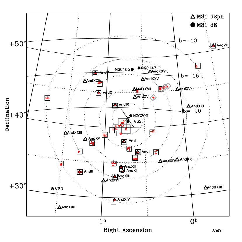
Figure 1.— Locations and orientations of the spectroscopic masks (red rectangles) included in the analysis (Section 2). The footprints of the KPNO/Mosaic (black), CFHT/MegaCam (dark gray), and Subaru/Suprime-Cam (light gray) images used to design the spectroscopic slit masks are also shown. The center of M31 is marked with an open circle, and the orientations of the major and minor axes of M31’s disk are denoted respectively by the long and short solid lines. The dwarf elliptical satellites of M31 are denoted by circles, and the dwarf spheroidal (dSph) satellites of M31 are denoted by triangles. The dotted circles denote radii of 2, 4, 6, 8, and 11 deg from M31’s center.

The photometric data are primarily from imaging observations obtained with the Mosaic Camera on the Kitt Peak National Observatory (KPNO) 4-m Mayall telescope. Photometric catalogs were derived from observations in the Washington system $M$ and $T_{2}$ filters and the intermediate-width DDO51 filter (Ostheimer, 2003). The observed magnitudes were transformed to $V$ and $I$ using the equations of Majewski et al. (2000).

Additional photometric data in the outer ($R_{\rm proj}$ $>30$ kpc) fields came from two sources. The photometry in field ‘d10’ was derived from $V$ and $I$ images obtained with the William Herschel Telescope (Zucker et al., 2007). Photometry for fields ‘streamE’ and ‘streamF’ was derived from $V$ and $I$ images obtained with the Suprime-Cam instrument on the Subaru Telescope (Tanaka et al., 2010).

Photometric catalogs for the innermost fields ($R_{\rm proj}$ $<30$ kpc) were derived from observations obtained with the MegaCam instrument on the 3.6-m CFHT. Images were obtained with the $g^{\prime}$ and $i^{\prime}$ filters. The observed stellar magnitudes were transformed to Johnson-Cousins $V$ and $I$ magnitudes using observations of Landolt photometric standard stars as described in Kalirai et al. (2006a).

The above photometric catalogs were used to design spectroscopic slit masks for use in the DEIMOS spectrograph on the Keck II telescope. Table 1 lists the filters used for each of the spectroscopic fields. Objects were assigned a priority for inclusion on the slit mask based on image morphology, their $I_{0}$ magnitude, and (when available) the probability of their being RGB stars at the distance of M31 based on their position in an ($M-T_{2}$, $M-$DDO51) color–color diagram (Palma et al., 2003; Majewski et al., 2005). The mask design process is described in detail by Guhathakurta et al. (2006). In the high-density inner regions of M31’s spheroid not all high priority M31 RGB candidates within the DEIMOS mask area can be included due to slit conflicts. In contrast, the low density outer fields contain a high fraction of low priority filler targets due to the paucity of M31 RGB candidates. The effect of this radial dependence of slit mask targets on the surface brightness estimates is discussed in Section 3.2.2.

Spectra were obtained over nine observing seasons (Fall 2002 – 2010) with the DEIMOS spectrograph on the Keck II 10-m telescope. The 1200 line mm^-1 grating, which has a dispersion of $\rm 0.33~{}\AA$ pixel^-1, was used for all observations. The slit width of 1″ yields a resolution of 1.6 Å FWHM. The typical wavelength range of the spectral observations is 6450 – 9150Å. This wavelength range includes the Ca ii triplet absorption feature at $\sim 8500$Å and the Na i absorption feature at 8190Å. Masks were observed for approximately 1 hr each, with modifications made for particularly good or bad observing conditions.

The spectra were reduced using modified versions of the spec2d and spec1d software developed at the University of California, Berkeley (Newman et al., 2012; Cooper et al., 2012). The spec2d routine is used to perform the flat-fielding, night-sky emission line removal and extraction of one-dimensional spectra from the two-dimensional spectral data. The spec1d routine cross-correlates the resulting one-dimensional spectra with template spectra to determine the redshift of the objects; the template library includes stellar spectra obtained with DEIMOS and galaxy spectra from the Sloan Digital Sky Survey (see Simon & Geha, 2007, for details). Each spectrum was visually inspected, and only stellar spectra with secure velocity measurements were included in the analyzed data set (Gilbert et al., 2006). Two corrections were applied to the observed velocities: (1) a heliocentric correction, and (2) a correction for imperfect centering of the star within the slit. The latter correction was calculated by measuring the observed position of the atmospheric $A$-band absorption feature relative to night sky emission lines (Simon & Geha, 2007; Sohn et al., 2007).

We are presenting data from 108 spectroscopic masks. These masks tareted $\sim 11000$ objects, and yielded successful velocity measurements from over 5800 stellar spectra (52.2%). The remainder of the targets were galaxy spectra (20.2%), spectra for which a velocity measurement was not possible due to insufficient signal-to-noise ratio (S/N) or a lack of strong spectral lines (24.2%), and a small fraction of catastrophic failures (3.4%).

2.2. Classification of M31 RGB Stars and Foreground MW Stars

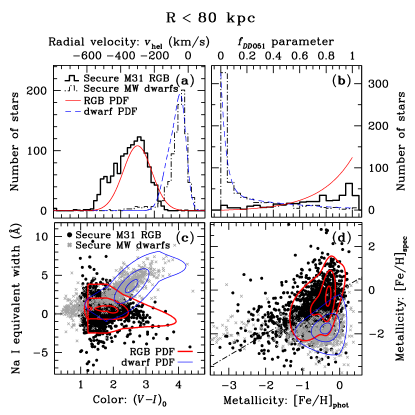
Figure 2.— Locations of stars in four of the five empirical diagnostics (Section 2.2; Gilbert et al., 2006): (a) line-of-sight velocity, (b) DDO51 parameter (Section 2.1), (c) Na i EW, and (d) spectroscopic versus photometric [Fe/H] estimates. Left 4 panels: stars identified as secure M31 red giants (classes +2 and +3) and MW dwarfs (classes $-2$ and $-3$) in fields from $R_{\rm proj}$ $\sim 8$ to 80 kpc. The majority of the stars come from the interior fields ($R_{\rm proj}$ $<30$ kpc). Right 4 panels: stars identified as secure M31 red giants and MW dwarfs in the outer fields ($R_{\rm proj}$ $\gtrsim 80$ kpc). The RGB and dwarf probability distribution functions shown in panels (a) and (b) are normalized to equal area. The PDF contours in panels (c) and (d) show the 90%, 50%, and 10% contours. Although significantly fewer in number and primarily metal-poor (as can be seen by comparing panel (d) in the left and right figures), stars identified as M31 RGB stars in the outer fields are consistent with the distribution of M31 RGB stars in the inner fields.

MW dwarf stars along the line of sight constitute a significant fraction of the observed stellar spectra even though the sample of spectroscopic targets consists primarily of objects that have been photometrically preselected to be M31 RGB candidates. Moreover, the line-of-sight velocity distributions of M31 halo RGB and MW dwarf stars overlap, and the velocity distribution of foreground MW stars has a tail that extends well into the velocity range typical of M31 halo stars. To estimate the surface brightness of a given M31 field, the relative fractions of stars in each of the two populations must be securely measured.

Individual stars are identified as M31 red giants or MW dwarfs using the method developed by Gilbert et al. (2006), to which readers are referred for full details of the technique. A combination of photometric and spectroscopic diagnostics are used to determine the probability an individual star is an M31 red giant or MW dwarf: (1) line-of-sight velocity ($v_{\rm los}$), (2) photometric probability of being a red giant based on location in the ($M-T_{2}$, $M-$DDO51) color-color diagram (when available; Table 1), (3) the equivalent width of the Na i absorption line (surface-gravity and temperature sensitive) versus $(V-I)_{0}$ color, (4) position in the ($I,\,V-I$) CMD and (5) spectroscopic (based on the EW of the Ca ii triplet) versus photometric (comparison to theoretical RGB isochrones) $\rm[Fe/H]$ estimates. Each diagnostic provides separation between M31 RGB stars and MW dwarf stars based on different physical parameters. A star’s location in each diagnostic is compared to empirical probability distribution functions (PDFs) to determine the likelihood ($L_{i}={\rm log}_{10}(P_{\rm RGB}/P_{\rm dwarf}$)) the star is an M31 red giant or MW dwarf (Figure 2); each PDF was determined using training sets of M31 red giant and MW dwarf stars (Gilbert et al., 2006). The likelihoods for each diagnostic are combined to give the overall likelihood, $\langle L_{i}\rangle$, the star is an M31 red giant or MW dwarf. Stars that are $\geq 3$ times more probable to be an M31 red giant than MW dwarf star ($\langle L_{i}\rangle$ $\geq 0.5$) are designated as secure M31 red giants (and vice versa for secure MW dwarf stars: $\langle L_{i}\rangle$ $\leq-0.5$); stars below this probability ratio threshold are designated as marginal M31 red giants ($0<$$\langle L_{i}\rangle$ $<0.5$) or MW dwarfs ($-0.5<$$\langle L_{i}\rangle$ $\leq 0$). The analysis is restricted to stars designated as secure M31 red giants or MW dwarfs because the secure categories suffer from the least contamination (Gilbert et al., 2007).

Figure 2 presents the position in the four most powerful diagnostics of secure M31 RGB and MW dwarf stars in fields interior (left panels) and exterior (right panels) to $R_{\rm proj}$ $\sim 80$ kpc. Very few stars are identified as secure M31 RGB stars in the outermost fields, however Figure 2 shows that those that are identified as M31 red giants are more consistent with the M31 RGB, rather than the MW dwarf, PDFs. The RGB stars in the outer fields ($R_{\rm proj}$ $\gtrsim 80$ kpc) are bluer (more metal-poor) than the average RGB star in the inner fields, as expected based on the observed metallicity gradient of M31’s stellar halo (Kalirai et al., 2006a; Chapman et al., 2006; Koch et al., 2008). However, their locations in the four diagnostics are consistent with the distribution of M31 RGB stars in the inner fields.

The noticeable asymmetry in the velocity distribution of M31 RGB stars within 80 kpc (Figure 2(a), left panel) is due to two effects. The first is the presence of stars associated with the giant southern stream in many of the south quadrant M31 halo fields. The velocity of the giant southern stream varies with $R_{\rm proj}$, but remains more negative than M31’s systemic velocity, $v_{\rm sys}^{\rm M31}=-300$  km s^-1 (Ibata et al., 2005; Guhathakurta et al., 2006; Kalirai et al., 2006b; Gilbert et al., 2009). The second effect is incompleteness in the secure sample of M31 RGB stars at the positive end of the M31 velocity distribution. The velocity diagnostic typically provides greater separation of the populations, and thus has intrinsically higher weight, than the other diagnostics. Thus the velocity region where the M31 and MW velocity distributions overlap tends to have a higher percentage of stars identified as marginal M31 RGB stars (for a full discussion, see the appendix of Gilbert et al., 2007).

2.2.1 Comparison of M31 RGB and MW Dwarf Star Samples

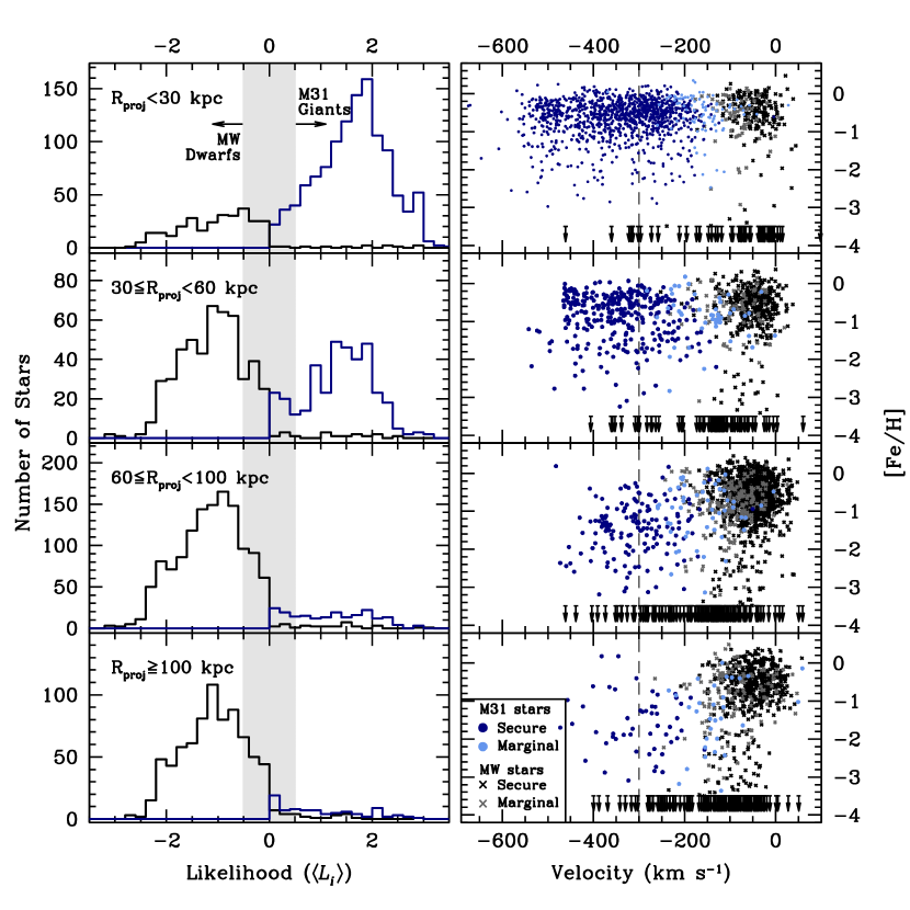
Figure 3.— Left: likelihood distribution (Section 2.2) of all observed stars as a function of projected distance from M31’s center. Blue histograms show the distribution of stars classified as M31 RGB stars, while black histograms denote foreground MW dwarf stars. The shaded area shows the region of likelihood space excluded from the analysis: stars that have likelihood values in this range are considered marginal identifications. Some stars are classified as MW dwarf stars even though $\langle L_{i}\rangle$ $\geq 0$. These are stars whose $V_{0},I_{0}$ magnitudes place them bluer than the most metal-poor isochrone by an amount greater than the photometric error (leading to an extrapolated $\rm[Fe/H]_{phot}$$\lesssim-3.5$, see right panels). Right: distribution of stars in the $\rm[Fe/H]_{phot}$–$v_{\rm los}$ plane. Marginal stars are those with $-0.5\leq$$\langle L_{i}\rangle$ $\leq 0.5$. Although the relative fraction of M31 RGB stars and MW dwarf stars changes with radius, the locus of M31 RGB stars in the $\rm[Fe/H]_{phot}$–$v_{\rm los}$ plane remains populated even at large projected distances ($R_{\rm proj}$ $\geq 100$ kpc) from M31’s center. M31’s systemic velocity is $v_{\rm los}=-300$  km s^-1.

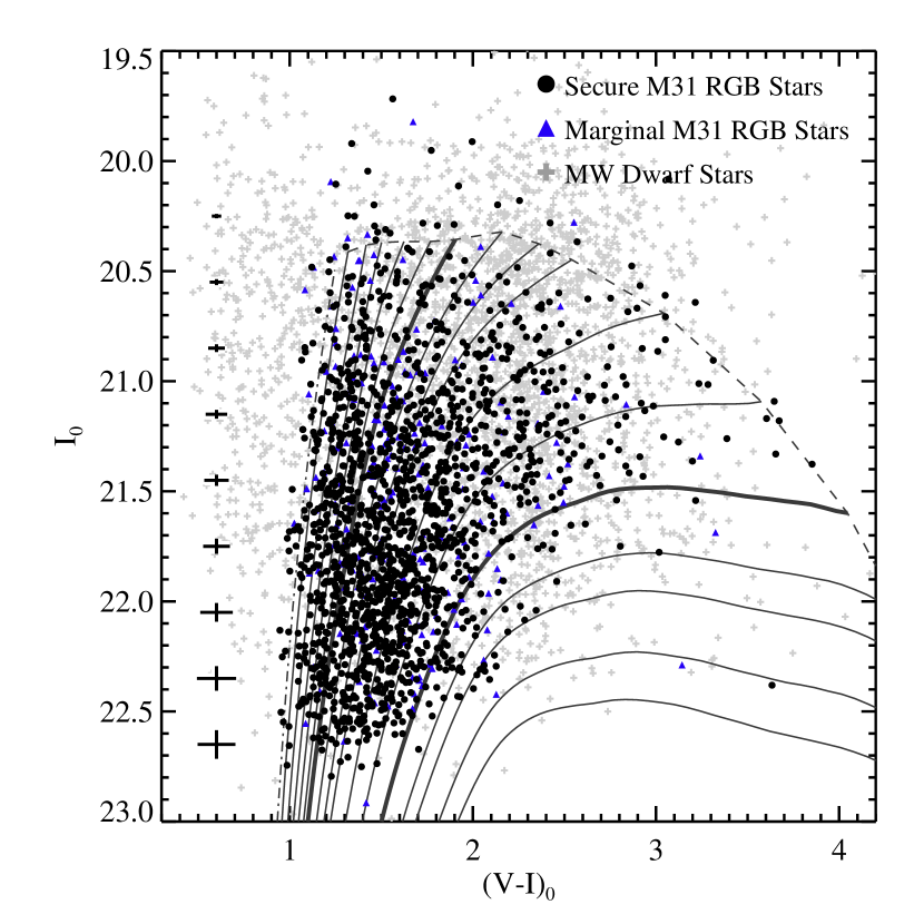
Figure 4.— $I_{0},(V-I)_{0}$ color–magnitude diagram for the spectroscopic sample, with theoretical isochrones of VandenBerg et al. (2006) ranging from [Fe/H]=$-2.3$ (left most) to $0.49$ (right most) overlaid (assuming an age of 10 Gyr and [$\alpha$/Fe]=0.0). The thick isochrones denote metallicities of [Fe/H]=$-1.0$ and $0.0$, while the dashed isochrone is for an age of 5 Gyr and [Fe/H]=$-2.3$. Stars classified as red giants at the distance of M31 trace the RGB isochrones, while stars classified as MW dwarf stars along the line of sight have a broader color distribution. Typical photometric errors as a function of $I$ magnitude are shown on the left: stars that are bluer than the most metal-poor isochrone by more than the typical photometric error are classified as MW dwarf stars (Section 2.2.1).

The left panels of Figure 3 show the distribution of stars in likelihood space. As discussed above, stars with marginal M31/MW classification (shaded region of left panels) tend to lie in the region of velocity space where the RGB and MW dwarf star PDFs overlap. Although the sample is divided into M31 and MW stars at $\langle L_{i}\rangle$=0, the true likelihood distributions of M31 ($\langle L_{i}\rangle$$>0$) and MW stars ($\langle L_{i}\rangle$$<0$) are expected to have tails that extend into negative and positive likelihood values, respectively. Restricting the sample to secure M31 ($\langle L_{i}\rangle$$\geq 0.5$) and secure MW ($\langle L_{i}\rangle$$\leq-0.5$) stars minimizes the contamination in the M31 and MW samples.

The right panels of Figure 3 display the location of stars in the plane defined by heliocentric line-of-sight velocity and photometric metallicity ($\rm[Fe/H]$). $\rm[Fe/H]$ values are determined by comparison of each star’s $I_{0}$ magnitude and $(V-I)_{0}$ color with a grid of theoretical RGB isochrones at the distance of M31 (Figure 4). For stars that are either slightly bluer than the bluest isochrone, or slightly above the TRGB, the metallicities are measured by extrapolating the grid, enabling a continuous mapping of the color-magnitude distribution of stars to $\rm[Fe/H]_{phot}$ space. Clearly, these isochrone based $\rm[Fe/H]_{phot}$ estimates are only physically meaningful for the bona fide M31 RGB stars. Regardless, in the $\rm[Fe/H]$–$v_{\rm los}$ plane, three distinct groups of stars are apparent in the sample. As discussed below, these groups represent RGB stars in the halo of M31, dwarf stars in the MW disk, and main-sequence turn off stars in the MW halo.

The M31 RGB star locus is centered at $v_{\rm los}=-300$  km s^-1 (the systemic velocity of M31) and spans a reasonable range of $\rm[Fe/H]_{phot}$ for RGB stars. Even in the most distant fields ($R_{\rm proj}$ $\geq 100$ kpc), the sample includes stars that are clearly located in the M31 locus.

The two MW dwarf star loci denote the two primary populations of MW contaminants expected in the survey. The MW dwarf locus at velocities $-150\lesssim v_{\rm los}\lesssim 50$  km s^-1 and relatively red colors (which translate into high $\rm[Fe/H]_{phot}$ estimates) is consistent with the properties expected for stars belonging to the disk of the MW.

The second MW dwarf locus has a wide spread in velocities ($-400\lesssim v_{\rm los}\lesssim 0$) and significantly bluer colors than either the M31 RGB stars or MW disk stars; indeed, the $(V-I)_{0}$ colors of these stars place them well to the blue of the RGB fiducials, and thus these stars are depicted with upper limits. This locus is consistent with the properties expected for main sequence turn-off stars at varying line-of-sight distances in the Galactic halo. The stars with $\langle L_{i}\rangle$$>0$ in Figure 3 that are classified as MW stars are part of this population. These stars’ velocities ($v_{\rm los}\lesssim-200$  km s^-1), combined with their blue colors [$(V-I)_{0}$$\lesssim 1$], typically lead to high ($\langle L_{i}\rangle$$>0$) likelihood values because the CMD, Na i EW, and [Fe/H] diagnostics have no discriminating power at these colors (Figure 2). Therefore, any star that is blue-ward of the most metal-poor isochrone by more than the typical photometric error is classified as an MW dwarf star (Figure 4; see Section 4.1.2 of Gilbert et al., 2006, for a more detailed discussion). It is possible that a small fraction of these could be M31 stars. Individual stars might have spurious photometric measurements, or they could be asymptotic giant branch stars or very metal-poor M31 halo red giants. However, the vast majority of these stars do appear to lie well-removed from the locus of M31 stars and to be part of a separate population of stars, with properties consistent with main sequence turn-off stars in the Galactic halo (Figure 3).

2.3. Identification of M31 Field Stars in Masks Targeting dSph Galaxies

The SPLASH survey includes an effort to measure the kinematical and chemical properties of M31’s dwarf satellite galaxies using spectroscopy of member stars (Kalirai et al., 2009, 2010; Tollerud et al., 2012). Thus, a number of the M31 spectroscopic fields presented here were designed to target dSphs in the halo of M31 (Table 1). The number of field stars belonging to M31’s stellar halo in the dSph masks is estimated following the technique used by Gilbert et al. (2009) (their Section 2.5.1, Figures 3 and 4). The distribution of stellar objects in velocity, metallicity, and sky position is used to isolate RGB stars that are likely part of M31’s stellar halo rather than members of the dwarf satellite. To classify the stars, we leverage the following three properties of the dSph galaxies: (1) they are generally compact enough to cover only a portion of the spectroscopic slit mask, (2) they have small velocity dispersions ($<10$  km s^-1), and (3) their member stars generally span a limited range of [Fe/H]. All RGB stars beyond the estimated King limiting radius of the dSph (McConnachie & Irwin, 2006; Martin et al., 2006; Majewski et al., 2007; Zucker et al., 2007; Collins et al., 2010) are designated as M31 field stars. RGB stars that are inside the limiting radius of the dSph but well removed from the tight locus in $v_{\rm los}$ – [Fe/H] space occupied by the dSph members are also designated as M31 field stars. Table 1 lists literature references for each dSph, where the distribution of stars and their membership is discussed in detail.

Although this procedure will miss M31 field stars that happen to fall both within the limiting radius of the dSph galaxy and in the region of $v_{\rm los}$ – [Fe/H] space occupied by the dSph members, the number of such M31 field stars is expected to be small. This is due in part to the fact that in each field, the dSph members span a very narrow range in velocity space compared to M31 halo stars. It is also due to the fact that the surface brightness of each dSph becomes increasingly dominant over the surface brightness of M31’s spheroid toward the center of the dSph, resulting in an increased likelihood that spectroscopic slits will be placed on a dSph member rather than an M31 field star.

3. Surface Brightness Estimates from M31 RGB Star Counts

The surface brightness of M31’s stellar halo is estimated from counts of spectroscopically confirmed M31 RGB stars (Section 2.2). The ratio of securely identified RGB stars ($N_{\rm M31}$) to securely identified MW dwarf stars ($N_{\rm MW}$) in a field is used to estimate M31’s stellar surface density. However, the density of foreground MW dwarf stars is not constant over the widely spaced spectroscopic fields. To account for this, the ratio of observed M31 RGB and MW dwarf stars is multiplied by the total expected surface density of MW stars in each field based on the Besançon Galactic population model ($N_{\rm BGM}$; Robin et al., 2003). The Besançon model counts are computed for the same magnitude and color range as the spectroscopic targets, and standard model parameters were used (models were drawn from a 1 deg² line-of-sight centered on each mask, including all ages and spectral types).

The scaled RGB counts are also corrected for two observational sources of bias: pre-selection of likely M31 RGB candidates using $M$, $T_{2}$, and DDO51 photometry ($c_{\rm DDO}$; Equation (3), Section 3.2.1), and unequal sampling of the RGB luminosity function ($c_{\rm LF}$; Equation (5), Section 3.2.2). Finally, the scaled and corrected RGB counts are converted to an $I$-band surface brightness. The normalization is determined by fitting for an overall normalization factor, $I_{\rm norm}$, that best matches our surface brightness estimates to the minor axis $I$-band surface brightness profile published by Courteau et al. (2011) (discussed further in Section 4.1). The normalization of the Courteau et al. profile is based on an $I$-band M31 image obtained by Choi et al. (2002). The surface brightness estimates are thus calculated as

$$\Sigma_{\rm I}=\Sigma_{\rm norm}-2.5\,{\rm log}_{10}\,\left[\frac{N_{\rm BGM}}{c_{\rm LF}\,c_{\rm DDO}}\,\frac{N_{\rm M31}}{N_{\rm MW}}\right].$$ (1)

Our method of estimating the surface brightness in each field is based on counting the relative numbers of M31 RGB and MW dwarf stars. Selecting only securely identified M31 RGB and MW dwarf stars (Section 2.2) is one way of doing this counting. We have also tested including the marginal M31 RGB and MW dwarf candidates, and have investigated fitting the M31 RGB and MW dwarf star likelihood distributions (Figure 3) to find the fraction of stars in each population. These alternate counting methods produce similar results. In the end however, our choice was influenced by the fact that restricting the sample to stars securely identified as belonging to one population or the other provides a clean sample from which to fit for kinematically cold components in each field.

3.1. Multiple Stellar Populations

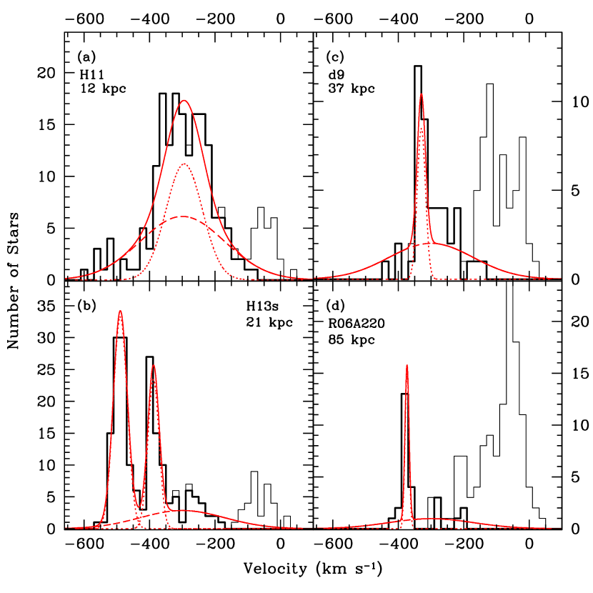
Figure 5.— Examples of multi-Gaussian fits (solid curves) to the velocity distribution of M31 stars (bold histogram) in fields with kinematically cold tidal debris. These fits are used to determine the fraction of stars belonging to M31’s kinematically hot spheroid (Section 3.1). Thin histograms denote the velocity distribution of all stars with recovered velocities. The fields shown span a range of projected distances from M31’s center and demonstrate the range of velocity dispersions measured for the kinematically cold components detected in individual fields (dotted curves), from $\sim 5$  km s^-1 (e.g., panel (d)) to $\sim 50$  km s^-1 (panel (a)). In some fields, more than one kinematically cold component is identified (panel (c)). In all fits, the mean velocity and dispersion of the Gaussian representing M31’s kinematically hot spheroid (dashed curves) is held fixed with parameters $\langle v\rangle^{\rm sph}$$=-300$  km s^-1 and $\sigma^{\rm sph}_{v}$$=129$  km s^-1 (Gilbert et al., 2007).

Many of the M31 halo fields targeted during the course of our Keck/DEIMOS survey show evidence of multiple kinematical components within the M31 halo population: i.e., one or more distinct, kinematically cold components associated with tidal debris in addition to M31’s kinematically broad spheroid (Guhathakurta et al., 2006; Kalirai et al., 2006b; Gilbert et al., 2007, 2009). The effect of these fields on the surface brightness profile of M31’s stellar halo will be discussed in detail below.

In fields with kinematically cold components (Table 1), the number of M31 stars in the dynamically hot component is calculated by multiplying the total number of M31 RGB stars in each field by the fraction of stars estimated to belong to the kinematically hot component. This fraction is determined by calculating maximum-likelihood multi-Gaussian fits to the stellar velocity distribution. The velocity distributions and associated maximum-likelihood fits of previously published fields with substructure are described in detail in the literature (Table 1).

Figure 5 shows examples of maximum-likelihood Gaussian fits in fields spanning a range of projected distances from M31’s center. The analysis implicitly assumes the presence of a dynamically hot component. In all fields with identified kinematical substructure, an underlying distribution of stars with a wide range of velocities is observed. However, this does not preclude the possibility that the broad distribution of stars (particularly in fields at larger radii) is a superposition of fainter, indistinct tidal debris features, rather than a dynamically well-mixed population of stars.

Only two of the new M31 halo fields have kinematical evidence of tidal debris. The velocity distribution of stars in these fields is presented in Figures 5(c) and (d). The substructure in field d9 is at $\langle v\rangle^{\rm sub}$$=-329.7^{+10.3}_{-6.6}$  km s^-1, with $\sigma^{\rm sub}_{v}$=$12.6^{11.0}_{-4.8}$  km s^-1; $29.1^{+14.0}_{-12.6}$% of stars in this field are estimated to belong to the kinematically cold component. This field is located at 37 kpc near M31’s major axis. The expected disk velocity at this location is $\sim-100$  km s^-1 (Ibata et al., 2005), making it unlikely that this feature is related to M31’s disk. The peak of MW stars with $v\sim-130$  km s^-1 may be related to the TriAnd overdensity in the MW halo; this feature is discussed further in Tollerud et al. (2012). The substructure in field R06A220 is at $\langle v\rangle^{\rm sub}$$=-373.5\pm 3.0$  km s^-1, with $\sigma^{\rm sub}_{v}$=$6.1^{+2.7}_{-1.7}$  km s^-1; $42$%$\pm 15$% of stars in this field are estimated to belong to the kinematically cold component.

Finally, we note that of the 39 fields presented here, only 4 specifically targeted tidal debris features: f207 and H13s targeted the giant southern stream, while the streamE and streamF fields were chosen to target photometric overdensities noted in Tanaka et al. (2010). The spectroscopic data show clear kinematical substructure in f207 and H13s, but there is no detectable kinematical substructure in the streamE or streamF fields. The remaining 35 fields were observed without prior knowledge of the presence of substructure in these fields, and thus represent a random sampling of the properties of M31’s stellar halo.

3.2. Primary Sources of Bias and Systematic Error

Since the surface brightness estimates are based on counts of spectroscopically confirmed samples of M31 RGB and MW dwarf stars, nonuniform spectroscopic target selection and variable observing conditions can significantly bias our measurements. Radially dependent systematic errors that affect the slope of the measured surface brightness profile are the most important to consider, since a purely empirical normalization is used to convert counts of confirmed M31 RGB stars and MW dwarf stars to surface brightness estimates. The surface brightness estimates are corrected for two sources of bias: selection of likely M31 RGB stars for spectroscopy based on Washington $M$, $T_{2}$, and DDO51 photometry, and the luminosity function (LF) of spectroscopic targets with successful velocity measurements. We describe each of these in detail below (Section 3.2.1 and sec:lumfun). Other sources of error that are not accounted for are discussed in Section 3.3.

3.2.1 DDO51 Selection Efficiency

Selection of likely M31 RGB stars using photometry in the Washington $M$ and $T_{2}$ filters and the DDO51 filter (Section 2.1) boosts the measured RGB/dwarf star ratios relative to fields without DDO51 photometry, and results in an offset in the surface brightness between fields with and without DDO51 photometry (Guhathakurta et al., 2005). Among the masks that benefit from DDO51-based target selection, masks at large $R_{\rm proj}$ contain a higher fraction of “filler” targets (that fail the DDO51 criterion for RGB stars) than masks at small $R_{\rm proj}$. Since many of these filler targets are MW dwarfs, this effect reduces the measured M31 RGB/MW dwarf ratio. Uncorrected, this would cause the derived radial surface brightness profile to be steeper (a more negative power-law index) than the true profile because a larger fraction of slits will target likely M31 RGB stars in DDO51-based masks at small $R_{\rm proj}$.

To correct for this effect, we estimate the factor by which the measured RGB/dwarf star ratios are increased by DDO51-based target selection. For each field a DDO51 selection function (DSF) is computed, defined as the ratio of the number of stars selected for inclusion on a spectroscopic mask ($N_{\rm target}$) to the number of stars available ($N_{\rm total}$), as a function of the DDO51 parameter ($f_{\rm DDO51}$; Figure 2(b)). The $f_{\rm DDO51}$ value measures the probability a star is an M31 red giant based on the Washington $M$, $T_{2}$, and DDO51 photometry (Palma et al., 2003; Majewski et al., 2005). The DDO51 correction factor ($c_{\rm DDO}$) is then defined as the ratio of two integrals: (1) the M31 RGB DDO51 probability distribution function (${\rm PDF_{RGB}}$, Section 2.2), convolved with the DDO51 selection function, and (2) the MW dwarf star DDO51 PDF (${\rm PDF_{dwarf}}$) convolved with the DDO51 selection function. The DDO51 PDFs for M31 and MW stars are shown in Figure 2(b).

$${\rm DSF}(f_{\rm DDO51})=\frac{N_{\rm target}(f_{\rm DDO51})}{N_{\rm total}(f_{\rm DDO51})}$$ (2)

$$c_{\rm DDO}=\frac{\int{\rm PDF_{RGB}}\,{\rm DSF}\,df_{\rm DDO51}}{\int{\rm PDF_{dwarf}}\,{\rm DSF}\,df_{\rm DDO51}}$$ (3)

The scaled M31 RGB counts in each field are divided by the DDO51 correction factor to account for differences in the DDO51 selection function between fields (Equation 1). For fields in which DDO51 photometry was not used for designing the masks, $c_{\rm DDO}$ is set to unity.

In field a0 ($R_{\rm proj}$ $\sim 30$ kpc), an inner field with many high priority targets, the DDO51-based selection of spectroscopic targets increased the measured RGB/dwarf ratio by a factor of 3.4. In the outermost fields where there are only a few bright stars ($I_{0}<23.0$) with high DDO51 parameters per mask, the DDO51-based selection increased the measured RGB/dwarf star ratio by a factor of 1.4.

The application of the DDO51 correction factor to the M31 RGB/MW dwarf ratio results in excellent agreement between the surface brightness estimates of fields with and without DDO51-based target selection at $R_{\rm proj}$ $\sim 30$ kpc (e.g., ‘mask4’ (no DDO51) and ‘a0’ and ‘a3’ (DDO51)). Interior to this radius fields did not have DDO51 photometry, while exterior to this radius the majority of the fields do have DDO51 photometry. The DDO51 correction factor removes the need to empirically adjust the normalizations of the surface brightness estimates for fields with and without DDO51 photometry.

3.2.2 Sampling of the Stellar Luminosity Function

In designing the spectroscopic masks, higher priority is given to brighter targets because recovering a velocity for these objects is more likely. However, a mask at large $R_{\rm proj}$ typically contains a higher fraction of faint targets than a mask at small $R_{\rm proj}$ due to the sparseness of stars in M31’s outer halo. For example, the number of $20.5<I_{0}<22$ targets is about twice that of $22<I_{0}<22.5$ targets in the $R_{\rm proj}$ $=30$ and 60 kpc fields a0 and a13, while these two magnitude ranges contain comparable numbers of targets in the outer fields m8 and m11 (at 120 and 165 kpc).

The M31 RGB $I$-band LF rises more steeply toward faint magnitudes than the MW dwarf $I$-band LF. Therefore the measured RGB/dwarf star ratio is expected to be higher in fields with a larger number of faint targets. If uncorrected, the larger number of faint targets in the outermost fields would bias the measured surface brightness profile to be flatter than the true profile. The amount of bias is limited because the spectroscopic targets span a relatively small apparent magnitude range and the radial velocity measurement fails for many stars with $I_{0}>22$, due to low S/N in the continuum.

In addition, variations in observing conditions (e.g., seeing and transparency) from one mask to another can lead to variations in the completeness function of radial velocity measurements. We attempted to minimize this effect by increasing the total exposure time for masks observed under sub-optimal conditions. Nevertheless there are field-to-field variations in the faint-end limiting magnitude of the spectra, which in turn leads to slight variations in the fraction of the LF that is included in our statistics.

To account for the above effects, we estimate the factor by which the measured M31 RGB/MW dwarf star ratio is increased in each field due to (1) a larger fraction of faint targets and/or (2) a fainter limiting magnitude for recovery of radial velocities from the spectra. The $I$ magnitude recovery function (IRF) is defined as the ratio of the number of stars with successful radial velocity measurements ($N_{\rm vel}$) to the total number of available targets in the photometric catalog ($N_{\rm total}$), as a function of $I$ magnitude. The correction factor ($c_{\rm LF}$) for each field is defined as the ratio of two integrals: (1) the M31 RGB LF convolved with the $I$ magnitude recovery function, and (2) the MW dwarf star LF convolved with the $I$ magnitude recovery function.

$${\rm IRF}(I)=\frac{N_{\rm vel}(I)}{N_{\rm total}(I)}$$ (4)

$$c_{\rm LF}=\frac{\int{\rm LF_{M31}}\,{\rm IRF}\,dI}{\int{\rm LF_{MW}}\,{\rm IRF}\,dI}$$ (5)

This is analogous to the procedure used for calculating the DDO51 selection efficiency factor (Section 3.2.1). The LF of M31 RGB stars is assumed to be $dN/dI=10^{0.3I_{0}}$, with a cutoff at $I_{0}=20.5$ corresponding to the tip of the RGB. The MW dwarf star LF is assumed to be a constantly rising function over the magnitude range of the spectroscopic survey; the slope is based on the Besançon Galactic population model (Robin et al., 2003).

The scaled M31 RGB counts in each field are divided by the correction factor $c_{\rm LF}$ to account for differences in the target selection and limiting magnitude of the spectroscopic observations in each field. The correction for sampling of the LF is a smaller correction than the correction for DDO51 selection: while the maximum variation in the DDO51 correction is a factor of $\sim 4$, the maximum variation in the LF correction is a factor of $\sim 2$.

3.3. Other Sources of Error

There are additional potential sources of error in the surface brightness estimates. We briefly discuss these and their possible impacts on the results below. In general, their effect on the measured surface brightness profile will be to add an extra source of noise in the measurements.

3.3.1 Masks Targeting dSphs

Some of the M31 fields target dSph galaxies in M31’s halo (Section 2.3). In the dSph masks, the precision with which the number of field stars in M31’s halo can be estimated depends on both the spatial extent of the dSph and the tightness of the locus of dSph member stars in the $v_{\rm los}$ – [Fe/H] plane. The amount of parameter space occupied by dSph members limits the parameter space where M31 field stars can be securely identified. In most cases, the parameter space spanned by the dSph is small compared to the parameter space spanned by M31 halo stars. The magnitude of the error in M31 RGB star counts thus introduced can be estimated by counting the number of M31 stars in the range of [Fe/H] values and width in velocity occupied by dSph members, but on the opposite side of M31’s Gaussian velocity distribution (i.e., if the dSph has a mean velocity of $-450$  km s^-1, one can count the number of M31 stars at $-150$  km s^-1 that would have been within the area of the $v_{\rm los}$ – [Fe/H] locus used to identify dSph stars). This additional source of error is generally found to be significantly smaller than the Poisson error; at the most, it is comparable in fields with very few M31 RGB stars.

3.3.2 Population Gradients

The PDFs used to identify M31 RGB stars were defined using a training set that was primarily drawn from fields in the inner, metal-rich regions of M31’s stellar halo. If the RGB classification method is significantly biased against selecting metal-poor stars, it is possible that large scale radial gradients in the metallicity of the halo population might bias the profile measurement. M31’s stellar halo does grow increasingly metal-poor with increasing radius (Kalirai et al., 2006a; Koch et al., 2008; Tanaka et al., 2010). A gradient in the age of the stellar population would also produce a bias, as changes in age produce similar color offsets as changes in metallicity for stars on the RGB.

However, there does not appear to be a significant bias against identifying metal-poor RGB stars as M31 stars in the sample. If the color-based and metallicity-based diagnostics biased the selection against blue, metal-poor stars, it would be most apparent in the velocity range $-200$ to $-150$  km s^-1. This is where the PDFs of the M31 RGB and MW dwarf velocity diagnostics overlap (Figure 2) and the effect of the velocity diagnostic on the overall likelihood is minimized. Figure 3 shows that the range of velocities spanned by stars classified as secure M31 red giants is similar whether the stars have $\rm[Fe/H]$$>-1$ or $\rm[Fe/H]$$<-1$.

3.3.3 Photometric Data Quality

Field-to-field variations in photometric accuracy and image quality lead to slight variations in the selection efficiency of M31 RGB spectroscopic candidates and the fraction of contaminating foreground MW dwarf stars and compact background galaxies observed on the spectroscopic masks. In general, the limiting magnitude of the photometric data is significantly fainter than that of the spectroscopic data, thus the error introduced by this effect is expected to be small compared to the Poisson errors.

3.3.4 Galactic Star-count Model

The surface density of MW dwarf stars predicted by the Besançon Galactic population model (Robin et al., 2003) only enters the final surface brightness estimates in a relative sense. It is used solely as a normalization factor ($N_{\rm BGM}$) to account for the changing density of MW dwarf stars across the survey, and a separate normalization factor is used to convert the surface densities to surface brightnesses (Section 4). Therefore, an absolute error in the total number of stars predicted by the Besançon model would not affect the resulting surface brightness estimates.

However, the Besançon model provides only a first order approximation for the true changes in MW stellar density across the footprint of the survey. A field-dependent error in the predicted projected density of MW dwarf stars could affect the resulting surface brightness profile.

If the Galactic latitude dependence of the number counts in the model is incorrect, this would result in a systematic error in the surface brightness estimates with a magnitude that varies as a function of the Galactic latitude of the field. A factor of two systematic error in the Besançon model between the highest and lowest Galactic latitude fields would result in a maximum systematic error of 0.75 mag; a factor of 1.5 error in the model counts would result in a maximum systematic error of 0.4 mag, which is comparable to the Poisson uncertainties for many of the fields.

However, there is not a direct correspondence between the projected distance of the fields from M31’s center and their Galactic latitude. Thus, the primary effect of a systematic error in the Galactic latitude dependence of the Besançon model number counts will be increased scatter in the surface brightness profile rather than a bias in the slope of the profile fit.

The Besançon model accounts only for the smooth components of the MW. However, the MW’s halo is known to have abundant substructure, and there is one known substructure, the Triangulum-Andromeda feature (Rocha-Pinto et al., 2004), which is in the direction of M31 and may affect some of the fields. Since the increased MW stellar density due to substructure is not accounted for by $N_{\rm BGM}$, the subsequent increase in observed MW star counts would result in a fainter M31 halo surface brightness estimate for a line of sight that passes through MW substructure. Therefore, the net effect of significant MW halo substructure will be increased scatter in the observed M31 halo surface brightness profile.

4. Surface Brightness Profile of M31’s Stellar Halo

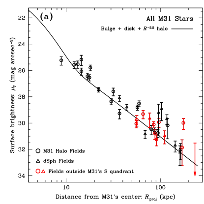
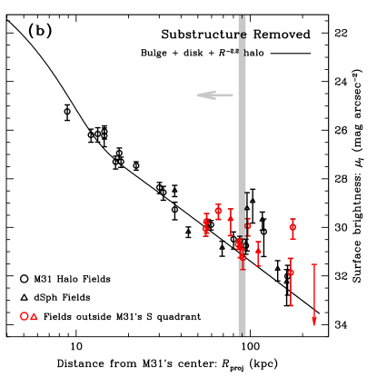
Figure 6.— Surface brightness profile of M31’s halo (Section 4), based on counts of spectroscopically confirmed RGB stars (Section 3). (a) Surface brightness estimates based on all M31 RGB stars in a given field. (b) Surface brightness estimates of the kinematically hot population of M31 RGB stars in each field (Section 3.1); due to the sparse nature of the outermost regions, tidal debris can only be identified in fields within $R_{\rm proj}$ $\lesssim 90$ kpc. The statistical subtraction of identified tidal debris features results in a smoother surface brightness profile for M31’s stellar halo. Error bars are the combined Poisson errors of the M31 RGB and MW dwarf star counts. For fields with substructure statistically removed, the error in the M31 RGB counts includes the uncertainty in the fraction of the population belonging to the kinematically hot component. The solid curve shows the maximum-likelihood minor axis surface brightness profile fit to the data and includes a Sérsic bulge, exponential disk, and power-law halo. The bulge and disk component parameters are set to those found to best fit a compilation of observations of M31’s light distribution by Courteau et al. (2011) (Section 4.1). Red points denote measurements from fields outside the southern quadrant of M31’s halo, confirming that M31’s stellar halo extends to large projected distances ($R_{\rm proj}$ $>150$ kpc) and follows the same power-law decline in surface brightness in all directions (Section 4.2.2).

Figure 6 displays the surface brightness estimates (Table 2) as a function of projected distance from M31’s center for each of the M31 fields shown in Figure 1. The surface brightness profile of M31’s stellar halo clearly extends to large projected distances ($R_{\rm proj}$ $\gtrsim 175$ kpc), with no evidence of a downward break in the profile (i.e., a transition to a steeper profile) at large radii.

To take into account the flattened profile of M31’s inner regions, the $R_{\rm proj}$ values of a small subset of the fields were converted to an effective radial distance along M31’s minor axis. This effective $R_{\rm proj}$ was calculated adopting a flattening of $b/a=0.6$ for $R_{\rm proj}$ $<30$ kpc, as measured for M31’s inner spheroid (Walterbos & Kennicutt, 1988; Pritchet & van den Bergh, 1994). No correction was necessary for the majority of the innermost fields ($R_{\rm proj}$ $\lesssim 30$ kpc), since most lie along M31’s minor axis. There are no strong observational constraints on the ellipticity of M31’s spheroid at large distances, therefore the spheroid of M31 is assumed to be spherical ($b/a=1$) beyond $R_{\rm proj}$ $=30$ kpc. This assumption is tested in Section 4.4.

Approximately a third of the fields targeted during the course of the SPLASH Keck/DEIMOS survey have conclusive kinematical evidence of tidal debris (Table 1; Guhathakurta et al., 2006; Kalirai et al., 2006b; Gilbert et al., 2007, 2009). In many cases, these kinematically cold components can be associated with known tidal debris features identified as photometric overdensities in star count maps. The left panel of Figure 6 shows the surface brightness estimates including all M31 halo stars, while the right panel shows the surface brightness estimates with the kinematically cold tidal debris features statistically subtracted (Section 3.1). In fields with kinematically cold tidal debris features, the error bars shown in Figure 6(b) include the uncertainty in the number of RGB stars belonging to the kinematically hot component, estimated from the maximum-likelihood fits to the field’s stellar velocity distribution (Section 3).

Statistical subtraction of tidal debris features reduces the scatter about the best-fit profile for the inner and medial fields; this effect is quantified below (Section 4.1). Significant scatter in the surface brightness estimates is noticeable at $R_{\rm proj}$ $\sim 90$ kpc (Figure 6), particularly in the right panel where tidal debris features have been statistically subtracted from the M31 RGB counts. The most distant field in which kinematically cold components can be identified in the spectroscopic data is at $R_{\rm proj}$ $=85$ kpc (Table 1). In fields at these large projected distances, there are typically $\lesssim 10$ secure M31 RGB stars per field. This makes discovering a tidal debris feature in the spectroscopic data prohibitively difficult unless it happens to dominate the line of sight. It is likely that there is substructure in some of these outer fields that cannot be identified as such due to the limited number of M31 stars. For example, fields ‘streamE’ and ‘streamF’ were placed on photometric overdensities identified as tidal debris features by Tanaka et al. (2010). However there is no definitive evidence of kinematically cold components in the spectroscopic data.

In the following subsections, we will discuss fits to the surface brightness profile of M31 with and without the inclusion of kinematically-identified tidal debris (Section 4.1) and explore the extent of M31’s stellar halo (Section 4.2) including an examination of the M31 RGB sample for signs of MW dwarf star contamination (Section 4.2.1). We also discuss the scatter of the data about the profile fit (Section 4.3), measure the ellipticity of M31’s stellar halo (Section 4.4), and compare our surface brightness estimates with M31 halo profile fits from the literature (Section 4.5).

4.1. Fits to Profiles With and Without Tidal Debris Features

The innermost data points ($R_{\rm proj}$$\lesssim 20$ kpc) are well within the region of M31’s halo where previous studies have found the profile to be consistent with an extension of M31’s bulge (Section 1). Therefore, we do not assume that contributions to the surface brightness from M31’s bulge and disk are non-negligible in these fields. A combined bulge, disk and power-law halo profile is fit to the M31 surface brightness estimates (Section 3) using a maximum-likelihood analysis. The intensity at a given radius is given by the functional form

$$I=I_{\rm b}(R_{\rm proj})+I_{\rm d}(R_{\rm proj})+I_{0}\left(\frac{1+(R_{*}/a_{h})^{2}}{1+(R_{\rm proj}/a_{h})^{2}}\right)^{\alpha}$$ (6)

where $I_{b}$ and $I_{d}$ represent the profile of M31’s bulge and disk along the minor axis, $-2\alpha$ is the halo’s two-dimensional power-law index, $a_{h}$ is a core radius inside of which the halo profile flattens, and $I_{0}$ and $R_{*}$ are normalization constants.

The recently published M31 surface brightness profile by Courteau et al. (2011) is used to fix the profiles of M31’s bulge ($I_{\rm b}$) and disk ($I_{\rm d}$). Courteau et al. analyzed photometric observations of M31’s inner regions, and compiled them with previously published surface brightness estimates to measure M31’s surface brightness profile along the major and minor axes. Here, we use their preferred minor-axis fit “U,” which included a Sérsic bulge ($n=1.9$, $R_{e}=0.73$ kpc), exponential disk (with scale length $R_{\rm d}=5.0$ kpc), and power-law halo. While this particular bulge/disk decomposition reproduces the observed surface brightness profile along the minor axis, the kinematical data in the innermost fields do not support the presence of such a prominent disk component (Gilbert et al., 2007); an attempt to include the kinematical data as a constraint on the inner minor-axis profile will be the subject of a future paper (Dorman et al., in preparation).

Although this work has significantly more data at large radii than Courteau et al., their minor axis profile has a much higher density of points out to 30 kpc. Their profile thus provides significantly more leverage for fitting the transition from M31’s inner regions (bulge and disk) to M31’s halo than the data presented here. Therefore, we adopt the core radius of $a_{h}=5.2$ kpc found for the Courteau et al. ‘U’ fit. This parameter sets the amplitude of the halo at small radii, and affects the radius at which the halo profile turns over. We adopt $R_{*}=30$ kpc, which is safely in the regime where the halo dominates the surface brightness profile; this choice is arbitrary and only affects the value of $I_{0}$ ($I_{h}(R_{*})=I_{0}$).

The total model intensity is compared to the surface brightness estimates to determine the power-law parameters (normalization, $I_{0}$, and power-law index, $-2\alpha$) that provide the maximum-likelihood fit to the data. The errors in the surface brightness estimates are used as weights when performing the maximum-likelihood analysis. When calculating the fit to the data set with kinematically identified tidal debris statistically removed (Figure 6(b)), the fit was restricted to the radial region over which each field has sufficient numbers of M31 stars to identify kinematical substructure ($R_{\rm proj}$ $<90$ kpc).

Given the significant scatter in the data, especially at large radius, we explore the effect of individual surface brightness estimates and their errors on the best-fit power-law index using Monte Carlo tests. Each trial was randomly drawn from the observed sample, allowing redrawing of individual data points. For each data point drawn, the number of M31 RGB and MW dwarf stars used to determine the surface brightness estimate are adjusted to a random deviate drawn from a Poisson distribution. The surface brightness estimates are then recalculated, and the maximum-likelihood power-law profile determined; 1000 trials were performed.

The data are best fit by a power-law profile with index $-2.2\pm 0.2$ and normalization $\mu_{0}=-2.5\,{\rm log}\,I_{0}=28.15\pm 0.15$ mag arcsec^-2. The quoted error estimate is the weighted standard deviation of the distribution of best-fit power-law indices from the Monte Carlo tests. This is formally consistent with the best-fit power-law found by Courteau et al. (index $-2.5\pm 0.2$ and $\mu_{0}=28.07\pm 0.05$ mag arcsec^-2). The best fit power-law profile index for the sample with kinematically cold tidal debris features removed is also $-2.2\pm 0.3$, fully consistent with the index found using all stars, but with a fainter halo normalization: $\mu_{0}=28.58\pm 0.14$ mag arcsec^-2.

The measured halo profiles are not very sensitive to the adopted bulge and disk profiles. Even if the surface brightness is assumed to be dominated by the halo for the full range of the data, and only a power-law component is fit, the best-fit index is $-2.4\pm 0.2$, consistent with the power-law fit including disk and bulge components. The power-law index is also fairly insensitive to the adopted core radius. If a smaller core radius, $a_{h}=2.7$ kpc, is adopted, consistent with an M31 halo measurement based on blue horizontal branch stars as tracers of the halo (Williams et al., 2012), the best-fit index is $-2.3\pm 0.2$.

The best-fit index is also not strongly dependent on the radial range used for fitting the data. If the radial range is restricted to $R_{\rm proj}$ $>20$ kpc, the best-fit power-law index is $-2.1\pm 0.3$ for the sample including all M31 stars; the best-fit power-law index is $-1.9\pm 0.4$ for $R_{\rm proj}$ $>35$ kpc. Although these best-fit values are shallower than the best-fit profile to all data points, the power-law indices are all consistent within the errors. The best-fit index for the sample with kinematical substructure statistically removed in the radial range $20<$ $R_{\rm proj}$ $<90$ kpc is also consistent: $-2.0\pm 0.5$.

4.2. Extent of M31’s Halo

4.2.1 Constraints on Contamination from MW Dwarf Stars

Figure 7.— Surface brightness of the M31 spectroscopic fields as a function of Galactic latitude. The left panel (a) shows measured surface brightness estimates, while the right panel (b) shows the scatter of the surface brightness estimates about the profile fit. The symbols used vary according to the radial distance of the field from M31’s center. The dotted line denotes the Galactic Latitude of M31’s center. If contamination from foreground MW disk stars was a significant factor in the M31 RGB surface brightness measurements, fields at lower absolute galactic latitude (closer to the disk of the MW) would be expected to have systematically higher surface brightness estimates than fields at comparable radii but higher absolute galactic latitude. Significant contamination would be most noticeable in the fields at large projected distances in M31’s halo, where the number of detected M31 RGB stars is small. No trend is seen in the data, indicating that foreground MW disk stars are not a significant source of contamination in the surface brightness estimates of the outer halo fields (Section 4.2.1).

M31 RGB stars are detected as far as $175$ kpc from the center of M31. The most distant field included in this paper, d7 ($R_{\rm proj}$$=230$ kpc), has objects identified as marginal M31 stars, but no secure M31 RGB star detections (Section 2.2). Given the large projected radial distances of the outermost fields, it is prudent to explore the effects that significant MW dwarf star contamination would have on the surface brightness estimates. Foreground MW dwarf star contamination consists of two physical groups of stars: those belonging to the MW’s disk and halo.

Dwarf stars in the disk of the MW have heliocentric line-of-sight velocities near $\sim 0$  km s^-1 (Figure 3). The surface density of MW disk stars increases as the galactic latitude of the field approaches 0^∘; this effect is significant over the area spanned by our spectroscopic survey (Figure 1). If MW disk stars are a significant source of contamination in the M31 RGB sample, fields closer to the MW disk (at lower absolute galactic latitude) should have systematically higher surface brightness estimates than fields farther removed from the MW disk. No clear trend is seen in the data (Figure 7, left panel), although each radial bin encompasses a rather large range of radii and hence intrinsic surface brightnesses.

The effect of the variation of surface brightness as a function of radius can be accounted for by subtracting the measured $\mu_{I}$ from the best fit profile (Figure 7, right panel). Intrinsic scatter of the M31 halo’s surface brightness about the profile fit will be independent of galactic latitude, producing a pure scatter plot. If significant contamination from MW disk stars was present in the sample, there would be a clear trend in $\mu_{\rm fit}-\mu_{\rm obs}$ as a function of Galactic latitude, with preferentially larger values at lower absolute Galactic latitudes. Based on the Besançon Galactic model (Robin et al., 2003), the density of MW stars along the line of sight is expected to increase by a factor of $\sim 8$ between the lowest and highest galactic latitude fields. If an approximately constant fraction of the MW disk stars present in each field creeps into the M31 RGB sample, the expected difference in surface brightness would be 2.2 magnitudes. Restricting the range of galactic latitudes to where the majority of the data lie ($-30<b<-15$) leads to an expected difference of 1.3 magnitudes. There is no apparent trend in the data even in the two outermost radial bins, let alone a trend this large. Therefore, we conclude that MW disk star contamination is not significantly affecting the M31 RGB surface brightness estimates. This also further demonstrates that the method of separating M31 RGB and MW dwarf stars (Section 2.2) is highly effective.

Bright, distant main sequence turn-off stars in the MW’s halo have a large range of velocities, and they can have very negative (M31-like) line-of-sight velocities (Figure 3). Their relatively blue colors make them particularly difficult to distinguish from M31 RGB stars, since the diagnostics described in Section 2.2 have less power at bluer colors (Figure 2). Foreground MW halo stars are expected to have approximately constant surface density across the area spanned by our M31 spectroscopic survey. Significant contamination from foreground MW halo stars in the M31 RGB halo sample would therefore manifest itself as a relatively constant (additive) surface brightness term, irrespective of radius. Naively, a constant term would simply be adjusted for in the empirical normalization of the data. However, given the spectroscopic selection function, we observe more MW halo stars on masks at large radii (because more filler targets are placed on the masks), and contamination is therefore expected to be larger in the outermost regions. If the term were large, it would therefore decrease the slope of the observed surface brightness profile.

At some large radius, this term would become larger than the signal of actual M31 RGB stars, and the measurements would become foreground-limited, which would manifest as a constant observed surface brightness with increasing radius. However, the surface brightness estimates continue to decrease with radius, consistent with the power-law profile (although with increasing scatter), out to the largest radii probed in our survey (Figure 6). Furthermore, the M31 halo sample and the likely MW halo stars (stars significantly bluer than the most metal-poor RGB isochrone, Figure 3) occupy distinct regions of the $\rm[Fe/H]$ – $v_{\rm los}$ plane.

Finally, a comparison of the kinematics of the M31 halo sample and the likely MW halo stars shows that the two have very different distributions at all radii: the M31 halo sample remains centered at the systemic velocity of M31, $v_{\rm los}=-300$  km s^-1, while the blue MW stars display a broad range of velocities approximately centered at the local standard of rest, $v_{\rm lsr}=-175$  km s^-1. This is shown quantitatively in Figure 8, which displays the surface brightness estimates of a subset of the M31 spectroscopic fields, calculated after splitting the M31 RGB sample at the systemic velocity of M31 ($-300$  km s^-1). Incompleteness in the sample, which is expected to occur at velocities overlapping the MW star velocity distribution (Figure 2, Gilbert et al., 2007) will cause points to fall above the one-to-one line, as surface brightness estimates calculated using the number of stars with $v>v_{\rm M31}$ will be fainter than estimates calculated using the number of stars with $v\leq v_{\rm M31}$. Conversely, contamination from MW halo stars will cause the points to fall below the one-to-one line. Since the same velocity PDFs are applied regardless of radius, incompleteness is expected to be roughly uniform, and is implicitly accounted for in the empirical normalization. Contamination from MW halo stars, however, is likely to be larger at faint surface brightnesses, where the ratio of M31 RGB stars to MW stars is low and the M31 RGB stars have relatively blue colors (Table 1, Figures 2 and 3). Reassuringly, the data points in Figure 8 are consistent with the one-to-one line even at faint surface brightnesses.

Figure 8.— Surface brightness estimates of a subset of the M31 spectroscopic fields, calculated after splitting the M31 RGB sample at the systemic velocity of M31 ($v_{\rm M31}=-300$  km s^-1). Only fields with a reasonable expectation of symmetry in the M31 velocity distribution are shown here; this excludes fields with kinematically identified tidal debris features and containing dwarf spheroidal galaxies (Table 1). The dotted line denotes the one-to-one line. MW halo stars have a broad range of velocities centered at $v\sim-175$  km s^-1. Thus, significant contamination from MW halo stars would result in surface brightness estimates calculated using the number of stars with $v>v_{\rm M31}$ to be brighter than estimates calculated using the number of stars with $v\leq v_{\rm M31}$, and the points would fall below the one-to-one line. However, the points are consistent with the one-to-one line, indicating that the sample is not significantly contaminated by MW halo stars at faint surface brightnesses (Section 4.2.1).

Combined, these tests indicate that the M31 RGB counts are not significantly contaminated by misidentified MW stars, and that we have not yet reached the radius at which the surface brightness estimates become foreground-limited.

4.2.2 Beyond the Southern Quadrant

Most previous studies of the surface-brightness profile of the outermost regions of M31’s stellar halo have been confined to the southern quadrant or M31’s southeast minor axis (Guhathakurta et al., 2005; Irwin et al., 2005; Ibata et al., 2007). Guhathakurta et al. (2005) presented a surface brightness profile extending out to $R_{\rm proj}$ $\sim 165$ kpc, generated from observations in fields in M31’s southern quadrant, primarily along M31’s SE minor axis. Irwin et al. (2005) likewise presented data along M31’s SE minor axis to projected distances of $R_{\rm proj}$ $=55$ kpc. Ibata et al. (2007) presented a photometric survey of M31’s entire southern quadrant out to $R_{\rm proj}$ $\sim 150$ kpc and detected substructure throughout a large portion of this region, much of it related to M31’s giant southern stream. These surface brightness profiles were all consistent with an $r^{-2}$ power-law stellar halo.

The stars in field m11, located on M31’s SE minor axis at a projected radial distance of $\sim 165$ kpc from M31’s center, are at a projected radial distance of $\sim 50$ kpc from the center of M33. Although it is more plausible that the stars in field m11 gravitationally belong to M31 given the relative sizes of the two galaxies, their velocity distribution does not rule out the possibility that they belong to M33 (Guhathakurta et al., 2005). In addition, a large H I bridge between M31 and M33 has been observed roughly along M31’s minor axis (Braun & Thilker, 2004), and a possible interaction between M31 and M33 has been posited based on relatively high star count densities observed extending from M33 in the direction of M31 (McConnachie et al., 2009).

It could therefore be argued that some or all of the outermost halo M31 RGB stars ($R_{\rm proj}$ $\gtrsim 100$ kpc) in fields in the southern quadrant may be part of large extended substructures connected either with the M31/M33 H I bridge or the giant southern stream, and not part of a global M31 halo extending to at least $170$ kpc. If this were the case, significant enhancements would be expected in the surface brightnesses of fields on the SE minor axis and in the S quadrant compared to fields in one of the other quadrants of M31’s stellar halo. The data do not show any evidence of such an overdensity (Figure 6).

PAndAS (McConnachie et al., 2009) has used the CFHT and the MegaCam instrument to survey the eastern, northern, and western quadrants of M31’s halo out to a maximum distance of $\sim 150$ kpc. McConnachie et al. (2009) presented the first evidence that the southern quadrant of M31’s stellar halo, although containing large amounts of substructure, still typified the extent and global structure of the full halo. Although they did not measure a surface brightness profile, they presented a stellar density map showing stars consistent with being M31 RGB stars from the SE minor axis counter-clockwise to the NW minor axis. They also found significant photometric substructure over the full survey area. Tanaka et al. (2010) presented the first surface brightness profile composed of stars beyond the southern quadrant, using Subaru/Suprime-Cam photometry of contiguous fields along the NW and SE minor axes out to $R_{\rm proj}$ $\sim 100$ kpc, and found reasonable consistency between the two profiles (Table 3).

The profile presented in Figure 6 confirms that M31’s stellar halo follows a consistent power-law profile regardless of position angle. Eleven of the M31 halo fields are on the northern side of the galaxy, spanning a large range of position angle and distance from M31’s center (Figure 1). The surface brightness estimates from these fields are shown in red in Figure 6 and are fully consistent with estimates from fields along the SE minor axis and in the southern quadrant. Furthermore, secure M31 RGB stars are found in both northern $R_{\rm proj}$ $\sim 170$ kpc fields. This supports the interpretation that the dynamically hot component in the southern quadrant fields are part of a global halo population that extends to at least 170 kpc from M31’s center.

4.3. Scatter of the Data about the Profile Fit: Effect of Substructure

Although the best-fit power-law indices are consistent for both surface-brightness profiles shown in Figure 6, the surface brightness estimates including all M31 halo stars show slightly more scatter at any given radius ($R_{\rm proj}$$\lesssim 90$ kpc) than the estimates that include only the fraction of stars belonging to the dynamically hot component of M31’s stellar halo. This is quantified in Figures 9(a) and (b). Statistical removal of stars associated with kinematically cold tidal debris features results in a decrease of a factor of 1.3 in the root-mean-square deviation of the data points about the best-fit profile. The rms value is computed using only data at $R_{\rm proj}$ $<90$ kpc since that is the radial limit at which kinematical substructure can be detected in the current data set.

The mean enhancement of the surface brightness in a field due to kinematically identified substructure is 1 mag; the root-mean-square deviation of the surface brightness enhancement in fields with kinematically identified substructure is 0.5 magnitudes. Figure 9(c) shows the aggregate effect of the inclusion of tidal debris features on the profile; it compares the surface brightness estimates including all stars with the best-fit profile to the surface brightness estimates with tidal debris statistically subtracted.

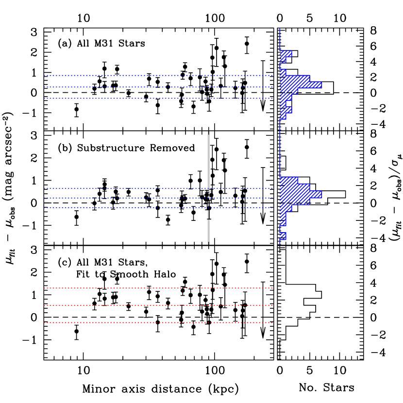
Figure 9.— Comparison of the scatter of the surface brightness estimates about the profiles shown in Figure 6, as a function of distance from the center of M31 (left panels) and in histogram form (right panels). (a) Values of $\Delta\mu$ (defined as $\mu_{\rm fit}-\mu_{\rm obs}$) for M31’s surface brightness profile including all M31 RGB stars (Figure 6(a)). The histograms show the scatter about the best-fit after controlling for the observational errors ($\Delta\mu$/$\sigma_{\mu}$). (b) Values of $\Delta\mu$ for the dynamically hot M31 RGB component and associated profile fit (Figure 6(b)); dynamically cold tidal debris features have been statistically removed. (c) The aggregate effect of substructure on the profile: values of $\Delta\mu$ calculated with the surface brightness estimates including all M31 RGB stars (Figure 6(a)) and the profile fit to the dynamically hot M31 RGB population (Figure 6(b)). Shaded histograms are for fields within $R_{\rm proj}$ $<90$ kpc, the outer limit at which we are able to identify substructure. In the left panels, the dotted lines show the mean and root-mean-square deviation from the mean of the $\Delta\mu$ values (blue: calculated for $R_{\rm proj}$ $<90$ kpc, red: calculated using all surface brightness estimates). Statistical removal of stars associated with dynamically cold tidal debris features in M31’s stellar halo results in a factor of 1.3 decrease in the rms deviation of the data from the best-fit profile (panels a and b, Section 4.3).

Next, we investigate whether the scatter of the surface brightness of individual sight lines in M31’s stellar halo increases with distance from M31. Physically, an increase in scatter with increasing $R_{\rm proj}$  could be caused by an increasing fraction of stars in the outer halo belonging to substructure. Observationally, an increase in scatter with $R_{\rm proj}$ could be due to the smaller number of stars observed in the outer fields: this simultaneously increases the error in the surface brightness measurements and reduces our ability to identify and remove substructure.

We can control for increasing error in the surface brightness estimates with increasing $R_{\rm proj}$ by analyzing the distribution of $\Delta\mu$/$\sigma_{\mu}$ values. If the scatter about the best fit profile is due solely to the observational errors, this distribution should have a standard deviation of order unity. The standard deviation is computed in three large radial bins: $R_{\rm proj}$ $\leq 30$ kpc, $30<$ $R_{\rm proj}$ $\leq 90$ kpc, and $R_{\rm proj}$ $>90$ kpc. The standard deviation is $\sim 2$ for the fit to fields including substructure, regardless of radius. For the surface brightness estimates with tidal debris features removed, the standard deviation is $1.5$ in both the $R_{\rm proj}$ $\leq 30$ kpc and $30<$ $R_{\rm proj}$ $\leq 90$ kpc bins, and $1.7$ for fields at $R_{\rm proj}$ $>90$ kpc, where the number of stars per field is insufficient to identify kinematically cold components.

There are several sources of observational error not captured in the formal error estimates that could increase the scatter in the surface brightness estimates. The fraction of stars in tidal debris features is determined by fitting multiple Gaussian components to a field’s velocity distributions (Section 3.1). However, Gaussians are likely an imperfect approximation of the true velocity distribution of the tidal debris: if there are more stars in the tails of the velocity distribution of tidal debris features than in the modeled Gaussians, this could lead to residual scatter about the profile. In addition, substructure in the MW’s halo or a large scale error in the accuracy of the Besançon model, which is used as a normalization factor, could also increase the scatter in the surface brightness estimates (Section 3.3).

4.4. Shape of M31’s Halo

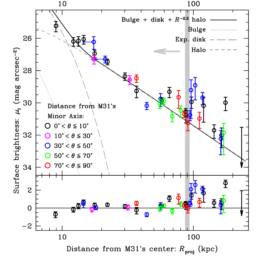
Figure 10.— Surface brightness profile of M31’s stellar halo; data points are color-coded by the field’s position angle from M31’s minor axis. Kinematically identified tidal debris features have been statistically subtracted from the surface brightness estimates in fields at $R_{\rm proj}$$<90$ kpc. Open points use $R_{\rm proj}$ for the abscissa, while the abscissa value of the smaller filled points (connected by arrows) is their projection onto the minor axis assuming a flattening of $b/a=0.6$ in M31’s inner spheroid ($R_{\rm proj}$ $<30$ kpc; Section 4; Walterbos & Kennicutt, 1988; Pritchet & van den Bergh, 1994). There is no apparent systematic offset of the surface brightness estimates as a function of angular position, indicating that the data are consistent with circular isophotes for M31’s outer stellar halo (Section 4.4).

The surface brightness estimates cover a large range of projected distances and position angles in M31’s stellar halo. If M31’s stellar halo has flattened isophotes with the same orientation as M31’s disk, data points at increasing position angles from the minor axis would have systematically higher surface brightness estimates than points at similar radii but near M31’s minor axis. If M31 had flattened isophotes with an orientation perpendicular to that of M31’s disk, the data would show systematic offsets in the opposite sense: data points with large position angles from the disk minor axis would have systematically fainter surface brightness estimates than data points at similar radii and near M31’s minor axis.

We investigate the data for evidence of such an effect in Figure 10. The surface brightness estimates and best-fit profile are for the sample with tidal debris features statistically removed to prevent bias of the measurement by strong, large-scale substructure (such as the giant southern stream). The surface brightness estimates are color-coded by their position angle from the minor axis (defined such that $\theta\leq 90$^∘). There is no significant, systematic offset of any subset of the data points from the profile fit, nor does there appear to be an increasing systematic offset with increasing position angle from the minor axis. The data appear to be consistent with a spherical halo in M31.

We quantify the degree of ellipticity of M31’s stellar halo via a maximum-likelihood analysis, under the constraints that the shape of the halo is assumed to be constant with radius and that the major axis of M31’s halo is aligned with either the major or the minor axis of M31’s disk. Each data point was projected along M31’s (disk) minor axis, assuming an axis ratio for the halo isophotes. The halo axis ratio is defined with respect to the M31 disk’s minor and major axes: a halo axis ratio smaller than one indicates the halo’s major axis is aligned with the disk major axis, while a halo axis ratio greater than one indicates the halo’s major axis is aligned with the disk minor axis. The best-fit profile was calculated as described in Section 4.1. The maximum-likelihood halo axis ratio was determined by comparing the $\chi^{2}$ values of each fit. Since the analysis is performed on the sample with kinematically identified substructure statistically removed, only fields with initial values of $R_{\rm proj}$$<90$ kpc are included in the profile fits and $\chi^{2}$ measurement; beyond this radius individual fields have too few stars to identify kinematical substructure.

The maximum-likelihood axis ratio for M31’s halo is $1.06^{+0.11}_{-0.9}$. This corresponds to elliptical isophotes with $b/a=0.94$, with the major axis of the halo aligned along the minor axis of M31’s disk, consistent with a prolate halo. Circular isophotes (consistent with a spherical halo) are within the 90% confidence limits, which encompass axis ratios of 0.96 to 1.17. The 99% confidence limits span a range of halo axis ratios of 0.92 and 1.25. The best-fit power-law index for a halo axis ratio of 1.06 is $-2.2$, the same as the power-law index of the nominal fit (Figure 6, Section 4.1).

Finally, based on previous work (Walterbos & Kennicutt, 1988; Pritchet & van den Bergh, 1994), we assumed an ellipticity in the surface brightness isophotes for fields with $R_{\rm proj}$$<30$ kpc for the nominal fits (Section 4). In practice, this significantly affected only two of the data points. The reader can see the effect of this assumption in Figure 10: the open points show the surface brightness estimates using the field’s $R_{\rm proj}$, while the smaller filled points (connected with arrows to the $R_{\rm proj}$ points) show the same surface brightness estimates, but using the effective radius along the minor axis assuming an isophotal flattening of $b/a=0.6$ (with the major axis aligned with the major axis of M31’s disk). Based on the results of the above analysis, we also tested the profile fits using $R_{\rm proj}$ for all data points, rather than assuming flattened isophotes in the inner regions, and found fully consistent fits with those quoted in Section 4.1. It is possible that the inner regions of M31’s stellar halo have a different ellipticity than the outer regions; however, given the limited number of data points at small radii, most of which are near the minor axis, we are unable to constrain the shape of M31’s inner halo separately from the shape of the outer halo.

4.5. Comparison with Previously Published Profiles

In the last several years multiple measurements of the surface brightness profile of M31’s outer halo have been made, primarily utilizing photometric observations along the southeast minor axis. These are summarized in Table 3. Although these studies largely use independent data sets and analysis, there is partial overlap in the footprints of several of the surveys; for example, seven of the 39 spectroscopic fields presented here overlap with the Tanaka et al. (2010) footprint. The Courteau et al. (2011) analysis makes use of the Irwin et al. (2005) data set and an updated Guhathakurta et al. (2005) data set.

Figure 11 shows the surface brightness estimates in log-linear form along with a range of literature fits to observations of M31’s outer halo ($R_{\rm proj}$ $\gtrsim 30$ kpc) surface brightness profile, including power-law profiles, Hernquist models (left panel), and exponential profiles (right panel). The Hernquist models provide reasonable fits to our data set; the smallest Hernquist model scale radius from the literature ($R_{s}=17.1$ kpc, Tanaka et al., 2010) is the most consistent with our data set over its full radial range. The data are consistent with the exponential fits only within relatively small radial ranges. A power-law profile or Hernquist model clearly provides a better fit than an exponential profile over the full radial range of the data.

The surface brightness estimates presented here extend to larger projected distances and cover a larger azimuthal range in M31’s stellar halo than any of the previously published profiles. Our technique of using counts of spectroscopically confirmed stars to estimate a surface brightness has an advantage at large projected distances over estimates based on photometric observations. In the sparsest outer regions of M31’s stellar halo, contaminants from the foreground (MW dwarf stars) and the background (distant unresolved galaxies) greatly outnumber the target M31 halo population. Given the large area of sky covered by M31’s stellar halo (over 20^∘ in diameter), and the strongly varying MW stellar density over this region of sky, the standard technique of identifying a comparison field and statistically subtracting it from the science image to remove contamination does not work. Spectroscopic observations identify individual objects as foreground MW stars, background galaxies, or M31 stars, enabling us to probe M31’s halo to large projected distances.

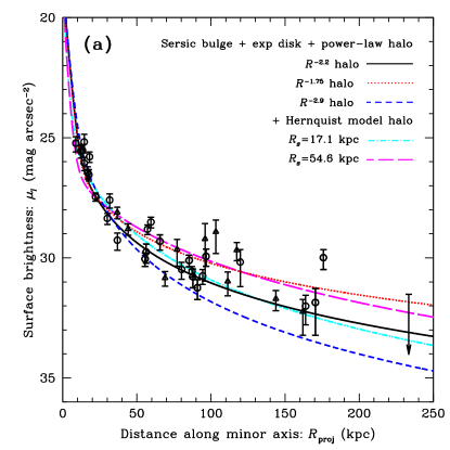
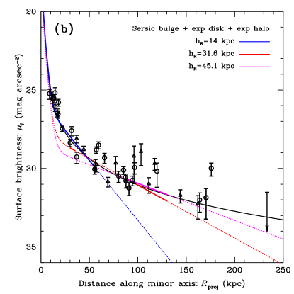
Figure 11.— Comparison of the surface brightness estimates of M31’s stellar halo (as in Figure 6(a)) with a range of profile fits from the literature, in log-linear form. In addition to the best-fit power-law profile to the data (black solid curve; same as in Figure 6(a)), alternative power-law indices and Hernquist models (left) and exponential fits (right) have been overlaid (Table 3, Section 4.5). (a) Alternative power-law indices for the outer halo component are overlaid on the data: $-2.9$ (red dotted curve) and $-1.75$ (blue dashed curve). Also shown are two Hernquist model fits from the literature. (b) Exponential fits with scale lengths of 14 kpc (blue curve; Irwin et al., 2005), 31.6 kpc (red curve; Ibata et al., 2007), and 45.1 kpc (magenta curve; Ibata et al., 2007). The exponential fits are shown as solid lines over the radial range in which they were measured, and as dotted lines outside this radial range. Hernquist models are consistent with the full range of the data, while exponential profiles are only consistent with the data in limited radial ranges.

5. Discussion

The density profiles found in simulations of stellar halo formation via accretion (e.g., Bullock & Johnston, 2005; Cooper et al., 2010; Font et al., 2011) are in good agreement with the measured surface brightness profile of M31’s stellar halo. Font et al. (2011) presented a study of $\approx 400$ stellar halos, simulated using a cosmological smoothed particle hydrodynamics code. Since stellar halo formation is a somewhat stochastic process, the exact properties of individual halos do differ. However, the median spherically averaged density profiles at large radii in the Font et al. (2011) simulations follow a power-law profile with $\rho(r)\propto r^{-3.5}$ (leading to a surface density distribution of $\Sigma(r)\propto r^{-2.5}$), in good agreement with that measured for the M31 halo surface brightness profile. The Bullock & Johnston (2005) simulations predicted stellar density profiles that closely followed Hernquist models with scale radii in the range $\sim 10-20$ kpc, also in good agreement with the observed surface brightness profile of M31 (Figure 11(a)). The published profiles typically show the aggregate density of the full stellar populations of the simulated stellar halos, including tidal streams, and are thus most comparable to the observed profile including all M31 stars.

The data show no evidence for a downward break in the surface brightness profile at large radii. Most $\Lambda$CDM-based predictions for stellar halo profiles (Bullock et al., 2001; Bullock & Johnston, 2005; Cooper et al., 2010) suggest that radially-averaged profiles of accreted stellar halos around M31-size galaxies should start to break rapidly around $r\sim 100$ kpc, taking on a steeper profile than that interior to $r\sim 100$ kpc. Of the 11 simulated stellar halos in Bullock & Johnston (2005), only one, halo 9, did not break to a steeper density profile at large radius; it followed a Hernquist profile with scale radius of 18 kpc, which is similar to the Hernquist scale radius for M31 measured by Tanaka et al. (2010) and shown to be consistent with the data in Figure 11. This simulated halo had an unusually large fraction of recent low-mass accretion/disruption events. The large spread in surface brightness in the fields at large radii may indicate that M31 has undergone a similar recent accretion history.

Simulations of stellar halo formation via accretion in a cosmological context also show that present-day stellar halos should contain many photometrically identifiable tidal streams (e.g., Bullock & Johnston, 2005; Johnston et al., 2008; Cooper et al., 2010). Thus, a study utilizing data from isolated sight lines through a stellar halo, like this one, should see significant scatter in the surface brightness profile due to the presence or absence of tidal streams along each line-of-sight. Furthermore, the simulations find that the contrast of stars in coherent tidal debris streams to stars in the diffuse stellar halo should become greater at large radii, as these streams are typically due to more recent accretion events. The inner regions of the simulated stellar halos tend to be built from early, relatively major mergers, and are more likely to have undergone significant phase-mixing resulting in a smoother stellar distribution.

The observations presented here provide one of the first direct observational tests of this aspect of the simulations. The surface brightness estimates show significant field-to-field variation in the stellar content of M31’s halo at all radii, beyond that expected based on the estimated observational errors. Tidal debris features are identified via stellar kinematics in $\sim 1/2$ of the fields within $R_{\rm proj}$ $\lesssim 90$ kpc. The tidal debris features generally comprise over half of the population in a given field, with the full range of measured substructure fractions extending from 29% in field d9 to 75% in field H13s. Bullock et al. (2001) estimated the expected field-to-field variation in star counts in stellar halos built via the accretion of satellites to be a factor of $\sim 2$ to 3 at large radii, in rough agreement with the observed field-to-field variation in our data set.

While removing kinematically identified substructure reduces the root-mean-square deviation of the data points about the profile fit, the amount of scatter in the data about the profile fit remains greater than that expected from the estimated observational errors, suggesting that the outer halo is composed of many small accreted objects that are unresolved into kinematically cold clumps or photometrically distinct streams at the limit of the currently available data. Interestingly, the data do not show evidence of an increasing fraction of coherent tidal streams with radius, as expected from simulations and discussed above. It is worth noting, however, that the inner regions of M31’s halo contain a high degree of substructure from the recent, relatively massive accretion event which formed the giant southern stream; in this sense, M31 may not be typical.

A detailed comparison of the fraction of substructure with radius, its effect on the observed surface brightness profile, and an analysis of the field-to-field variation with that predicted in simulations should yield interesting constraints on the merger history of M31 and the properties of its former satellite populations (e.g., the LF), and may help to provide constraints on the assumptions for satellite properties used in simulations. This kind of detailed comparison is currently only possible in M31. M31’s proximity allows us to obtain detailed observations of the entire stellar halo, including the crucial kinematical data that allows us to separate tidal debris features from the smoother underlying stellar halo in individual lines-of-sight.

Interestingly, recent simulations employing smoothed particle hydrodynamics (and thus explicitly simulating the evolution of the baryons, including star formation) imply that a significant fraction of the stellar population in the inner regions of stellar halos may be formed in the host galaxy potential (Zolotov et al., 2009; Font et al., 2011; McCarthy et al., 2012). This could have several effects on the observed stellar distribution, including naturally providing an inner spheroid ($R_{\rm proj}$ $\lesssim 10$ – 30 kpc) with different structural and chemical properties than the outer spheroid, as has been observed in M31. Indeed, McCarthy et al. (2012) showed that in their simulations, the in situ stellar component results in a significantly flattened, oblate stellar density distribution in the inner regions (semi-minor to semi-major axis ratio of $b/a\sim 0.3$) that slowly becomes more spherical with increasing radius, reaching $b/a\sim 1$ at radii of $\sim 100$ kpc. The inner regions ($R_{\rm proj}$ $\lesssim 30$ kpc) of M31’s spheroid have been shown to have flattened surface brightness contours ($b/a\sim 0.6$; Walterbos & Kennicutt, 1988; Pritchet & van den Bergh, 1994), while the outer regions appear consistent with circular surface brightness contours ($b/a\sim 1.0$; this work). In contrast, the $N$-body plus semi-analytic models, in which star particles are ‘painted’ onto the dark matter distribution, tend to find a prolate density distribution for the inner stellar halo (Cooper et al., 2010).

Detailed comparisons of the observed distribution of stars in M31’s stellar halo with simulations of halo formation will be crucial for constraining the fraction of stars in stellar halos formed in situ. Spectroscopic studies such as this one will have a natural advantage for such comparisons because the spatially diffuse, kinematically hot component can be separated from and compared to the tidal debris in every field.

6. Conclusions

We have analyzed data in 38 lines of sight in M31’s stellar halo, including all quadrants and ranging from 9 to 230 kpc in projected distance from M31’s center. Spectroscopic observations of stars were obtained in a total of 108 multi-object slit masks. The stellar spectra were used to identify samples of M31 RGB stars and MW dwarf star contaminants, and to identify M31 stars belonging to tidal debris features. Counts of M31 RGB stars and MW dwarf stars were used to determine the surface brightness in each line-of-sight, yielding a surface brightness profile of M31’s stellar halo.

We expand upon our main conclusions below. In brief, our conclusions are as follows.

• We present a clear detection of M31’s stellar halo to projected distances of 175 kpc from M31’s center.

• Multiple tests indicate there is minimal contamination from misclassified foreground MW stars in the sample of M31 RGB stars.

• The surface brightness profile follows a power-law with an index of $-2.2$.

• The statistical subtraction of tidal debris allows us to investigate its effect on the measured surface brightness profile.

We present a clear detection of M31’s stellar halo to projected distances of 175 kpc from M31’s center (Figure 6). Our data set includes lines-of-sight spread throughout all quadrants of M31’s stellar halo, covering a range of radii. The data show that M31’s stellar halo extends to at least $\sim 2/3$ of M31’s estimated virial radius ($\sim 260$ kpc; Seigar et al., 2008). In aggregate, a large spread in the velocities of M31 halo stars is observed even in fields at large projected distances from M31’s center ($R_{\rm proj}$$>100$ kpc, Figure 3).

Multiple diagnostic tests indicate there is minimal contamination from misclassified foreground MW stars in the sample of M31 RGB stars. The spectroscopic data enable us to remove foreground and background contaminants, allowing us to trace M31’s stellar halo to fainter surface brightnesses, and larger radii, than studies based on photometry alone. Tests show that using the Gilbert et al. (2006) likelihood method to identify M31 RGB and MW dwarf stars does an excellent job of cleanly separating the two populations (Section 4.2.1, Figures 7 and 8). If the M31 RGB sample was significantly contaminated by MW disk stars, there would be a strong dependence on the surface brightness of fields as a function of Galactic latitude. No such dependence is seen in the data. The density of MW halo stars is expected to be relatively uniform across the face of M31, so significant contamination would lead to a constant surface brightness measurement. Our sample instead displays a systematic fall off with projected distance from M31’s center. Furthermore, surface brightness estimates in individual fields calculated by splitting the M31 sample at the systemic velocity of M31 are consistent even at faint surface brightnesses, indicating that contamination from MW halo stars is not significant. Even at large radii ($R_{\rm proj}$$>100$ kpc) there are stars with properties consistent with M31 RGB stars rather than MW halo or disk stars (Figures 2 and 3).

The surface brightness profile follows a power law with an index of $-2.2$. This is consistent with what previous studies that have mainly targeted the southern quadrant of M31 have found. This work establishes that an $\sim r^{-2}$ power-law profile is a good description of M31’s outer halo ($R_{\rm proj}$ $\gtrsim$ 20 – 30 kpc) regardless of quadrant or radius. The data show no evidence of a downward break in the profile at large radii ($R_{\rm proj}$ $\gtrsim 100$ kpc). Since the fields cover a large range in both radii and position angle around M31, they provide leverage on the shape of M31’s halo. The best-fit elliptical isophotes have $b/a=0.94$, with the major axis of the halo aligned along the minor axis of M31’s disk, consistent with a prolate halo. However, a value of $b/a=1$ is well within the 90% confidence limits of the fit, so the data are consistent with a spherical halo.

The statistical subtraction of tidal debris allows us to investigate its effect on the measured surface brightness profile. The ability to remove stars associated with tidal debris from individual lines of sight is a unique advantage of our spectroscopic survey over photometric surveys of M31’s stellar halo. There are enough stars per field to discover kinematically cold tidal debris features for fields with $R_{\rm proj}$ $\lesssim 90$ kpc. Tidal debris features are identified using kinematics in $\sim 1/3$ of the spectroscopic fields ($\sim 1/2$ of fields with $R_{\rm proj}$ $\lesssim 90$ kpc). In fields with substructure, the mean enhancement of the surface brightness is 1 mag, with a root-mean-square deviation of the sample about the best-fit profile of 0.5 mag. The scatter about the mean surface brightness profile decreases once kinematically identified tidal debris features are statistically subtracted. This implies that there is a comparatively diffuse stellar component to M31’s stellar halo out to at least $R_{\rm proj}$ $\sim 90$ kpc, with relatively prominent tidal debris features superimposed.

Table 1Basic Results of Spectroscopic Observations.

Field	No.	Mean	Filters	No.	No.	No.	Kinematically	Dwarf	Reference
	Masks	Projected		Stellar	Secure	Secure	Identified	Satellite
		Radius		Spectra	M31	MW	Substructure	Field
		(kpc)			RGB	Dwarf
					Stars	Stars
f109	1	9	$g^{\prime}$, $i^{\prime}$	186	148	13			(1)
H11	2	12	$g^{\prime}$, $i^{\prime}$	206	165	21	Yes		(1)
f116	1	13	$g^{\prime}$, $i^{\prime}$	171	140	18	Yes		(1)
f115	1	15	$g^{\prime}$, $i^{\prime}$	136	95	20			(1)
f207	1	17	$g^{\prime}$, $i^{\prime}$	123	113	9	Yes		(2)
f135	1	17	$g^{\prime}$, $i^{\prime}$	133	93	24	Yes		(1)
f123	1	18	$g^{\prime}$, $i^{\prime}$	126	96	28	Yes		(1)
H13s	2	21	$g^{\prime}$, $i^{\prime}$	212	177	30	Yes		(3) (2)
f130	3	22	$g^{\prime}$, $i^{\prime}$	201	98	70			(1)
a0	3	30	$M$, $T_{2}$, DDO51	120	70	34			(1)
a3	3	33	$M$, $T_{2}$, DDO51	88	78	17	Yes		(4) (2)
mask4	1	37	$g^{\prime}$, $i^{\prime}$	57	13	37
d9	2	37	$M$, $T_{2}$, DDO51	133	46	38	Yes	And IX	(5)
d1	2	44	$M$, $T_{2}$, DDO51	185	44	41	Yes	And I	(2) (6)
m4	5	57	$M$, $T_{2}$, DDO51	160	46	93	Yes		(2)
R04A240	3	56	$M$, $T_{2}$, DDO51	123	19	87
R04A338	3	56	$M$, $T_{2}$, DDO51	101	9	72
a13	4	58	$M$, $T_{2}$, DDO51	114	42	56	Yes		(2)
streamE	2	66	$V$, $I$	117	15	71
d3	3	69	$M$, $T_{2}$, DDO51	192	15	104		And III	(2) (6) (5)
d10	2	77	$V$, $I$	100	5	49		And X	(7) (6) (5)
a19	4	80	$M$, $T_{2}$, DDO51	142	11	115
R06A220	3	85	$M$, $T_{2}$, DDO51	146	26	102	Yes
m6	5	87	$M$, $T_{2}$, DDO51	235	28	174
R06A310	3	88	$M$, $T_{2}$, DDO51	169	9	135
R06A040	3	91	$M$, $T_{2}$, DDO51	197	8	161
b15	5	94	$M$, $T_{2}$, DDO51	144	15	103
d12	1	96	$M$, $T_{2}$, DDO51	12	2	7		And XII	(5)
streamF	3	97	$V$, $I$	170	11	118
d11	1	103	$M$, $T_{2}$, DDO51	19	4	14		And XI	(5)
d5	3	111	$M$, $T_{2}$, DDO51	167	6	56		And V	(5)
d13	5	117	$M$, $T_{2}$, DDO51	62	14	26		And XIII	(5)
m8	2	120	$M$, $T_{2}$, DDO51	36	3	25
d2	11	144	$M$, $T_{2}$, DDO51	654	8	98		And II	(6) (5)
R11A170	3	162	$M$, $T_{2}$, DDO51	117	3	45		And XIV	(8) (6) (5)
m11	4	164	$M$, $T_{2}$, DDO51	117	4	93
R11A080	2	170	$M$, $T_{2}$, DDO51	127	2	103
R11A305	2	176	$M$, $T_{2}$, DDO51	147	8	123
d7	2	233	$M$, $T_{2}$, DDO51	217	0	26		And VII	(6) (5)

Table 2Surface Brightness Estimates Based on a Spectroscopically Confirmed Sample.

Field	R.A.	Decl.	$\mu_{I}$
	(hh:mm:ss)	(∘:′:″)	(mag arcsec-2)
	(J2000)	(J2000)	All	Substructure
			Stars	Removed
f109	00:45:46.75	40:56:53.8	$25.23^{+0.37}_{-0.28}$
H11	00:46:21.02	40:41:31.3	$25.56^{+0.29}_{-0.23}$	$26.19^{+0.30}_{-0.24}$
f116	00:46:54.53	40:41:29.5	$25.52^{+0.31}_{-0.24}$	$26.15^{+0.33}_{-0.25}$
f115	00:47:32.71	40:42:00.9	$26.06^{+0.31}_{-0.24}$
f207	00:43:42.64	40:00:31.6	$25.17^{+0.46}_{-0.32}$	$26.22^{+0.46}_{-0.32}$
f135	00:46:24.88	40:11:35.5	$26.44^{+0.28}_{-0.22}$	$27.30^{+0.30}_{-0.23}$
f123	00:48:05.57	40:27:16.3	$26.54^{+0.26}_{-0.21}$	$26.94^{+0.26}_{-0.21}$
H13s	00:44:14.76	39:44:18.2	$25.79^{+0.24}_{-0.20}$	$27.30^{+0.23}_{-0.19}$
f130	00:49:08.02	40:14:39.8	$27.46^{+0.18}_{-0.16}$
a0	00:51:43.79	39:53:47.7	$28.36^{+0.25}_{-0.21}$
a3	00:48:10.52	39:07:04.7	$27.59^{+0.34}_{-0.26}$	$28.56^{+0.32}_{-0.25}$
mask4	00:54:08.34	39:41:51.7	$29.27^{+0.42}_{-0.30}$
d9	00:52:50.58	43:11:09.0	$28.11^{+0.27}_{-0.22}$	$28.48^{+0.26}_{-0.21}$
d1	00:46:01.28	38:03:06.9	$28.80^{+0.27}_{-0.21}$	$30.18^{+0.24}_{-0.20}$
m4	01:00:10.49	38:49:45.7	$28.81^{+0.22}_{-0.18}$	$29.83^{+0.19}_{-0.16}$
R04A240	00:24:05.34	39:21:06.3	$30.05^{+0.32}_{-0.24}$
R04A338	00:34:57.17	45:07:26.8	$29.76^{+0.47}_{-0.33}$
a13	00:42:06.13	37:01:40.3	$28.51^{+0.25}_{-0.20}$	$29.89^{+0.21}_{-0.18}$
streamE	00:22:11.76	44:11:57.9	$29.31^{+0.36}_{-0.27}$
d3	00:35:51.72	36:24:34.6	$30.84^{+0.35}_{-0.26}$
d10	01:06:37.66	44:49:04.6	$29.65^{+0.69}_{-0.42}$
a19	00:37:30.62	35:33:28.1	$30.48^{+0.41}_{-0.30}$
R06A220	00:22:23.41	36:25:30.5	$30.11^{+0.27}_{-0.22}$	$30.70^{+0.21}_{-0.18}$
m6	01:08:55.43	37:35:59.3	$30.56^{+0.25}_{-0.20}$
R06A310	00:16:10.87	45:25:59.3	$30.79^{+0.46}_{-0.32}$
R06A040	01:06:22.60	46:18:29.6	$31.25^{+0.49}_{-0.34}$
b15	00:53:14.13	34:52:38.6	$30.75^{+0.35}_{-0.27}$
d12	00:47:35.72	34:20:59.0	$29.21^{+1.76}_{-0.64}$
streamF	00:12:05.81	45:33:48.1	$29.94^{+0.41}_{-0.30}$
d11	00:46:29.15	33:50:05.0	$28.91^{+0.91}_{-0.49}$
d5	01:10:21.00	47:39:11.7	$30.98^{+0.61}_{-0.39}$
d13	00:51:56.75	33:00:22.0	$29.68^{+0.44}_{-0.31}$
m8	01:18:23.72	36:15:27.9	$30.18^{+1.03}_{-0.52}$
d2	01:16:25.19	33:26:10.7	$31.71^{+0.50}_{-0.34}$
A170	00:51:41.82	29:40:49.4	$32.24^{+0.98}_{-0.51}$
m11	01:29:56.91	34:17:10.9	$32.01^{+0.78}_{-0.45}$
R11A080	01:47:09.12	43:20:24.0	$31.86^{+1.36}_{-0.59}$
R11A305	23:44:10.24	48:05:56.0	$29.99^{+0.49}_{-0.34}$

Table 3Recent Profile Measurements of M31’s Halo.

Study	$R_{\rm min}$	$R_{\rm max}$	Power-law	Data type	Notes
	(kpc)	(kpc)	Index	(Fit Type)
			(Scale Length)
Guhathakurta et al. (2005)	30	165	$-2.3$	Spectroscopic	S quadrant
					(included 10 of the fields presented here)
Irwin et al. (2005)	20	55	$-2.3$	Photometric	SE minor axis
			(14)	(Exponential)
Ibata et al. (2007)	30-35	90-130	$-1.9\pm 0.12$	Photometric	SE minor axis
			($31.6\pm 1.0$)	(Exponential)
			($54.6\pm 1.3$)	(Hernquist)
	90	130	($45.1\pm 6.0$)	(Exponential)
			($53.1\pm 3.5$)	(Hernquist)
Tanaka et al. (2010)	20	100	$-1.75\pm 0.13$	Photometric	SE minor axis
			($22.4\pm 2.3$)	(Exponential)
			($31.7\pm 6.7$)	(Hernquist)
	20	100	$-2.17\pm 0.15$		NW minor axis
			($18.8\pm 1.8$)	(Exponential)
			($17.1\pm 4.7$)	(Hernquist)
Courteau et al. (2011)	0	165	$-2.5\pm 0.2$	Photometric and	SE minor axis preferred fit
				Spectroscopic	(included 11 of the fields presented here)
Williams et al. (2012)	2	35	$-2.6^{+0.3}_{-0.2}$	Photometric	BHB stars used as tracers of the halo
This work	9	176	$-2.2\pm 0.2$	Spectroscopic	All quadrants, all M31 stars
	35	176	$-1.9\pm 0.4$		All quadrants, all M31 stars
	9	90	$-2.2\pm 0.3$		Tidal debris statistically subtracted

References

- Bellazzini et al. (2003) Bellazzini, M., Cacciari, C., Federici, L., Fusi Pecci, F., & Rich, M. 2003, A&A, 405, 867
- Braun & Thilker (2004) Braun, R., & Thilker, D. A. 2004, A&A, 417, 421
- Brown et al. (2008) Brown, T. M., Beaton, R., Chiba, M., Ferguson, H. C., Gilbert, K. M., Guhathakurta, P., Iye, M., Kalirai, J. S., Koch, A., Komiyama, Y., Majewski, S. R., Reitzel, D. B., Renzini, A., Rich, R. M., Smith, E., Sweigart, A. V., & Tanaka, M. 2008, ApJ, 685, L121
- Brown et al. (2003) Brown, T. M., Ferguson, H. C., Smith, E., Kimble, R. A., Sweigart, A. V., Renzini, A., Rich, R. M., & VandenBerg, D. A. 2003, ApJ, 592, L17
- Brown et al. (2007) Brown, T. M., Smith, E., Ferguson, H. C., Guhathakurta, P., Kalirai, J. S., Rich, R. M., Renzini, A., Sweigart, A. V., Reitzel, D., Gilbert, K. M., & Geha, M. 2007, ApJ, 658, L95
- Brown et al. (2006) Brown, T. M., Smith, E., Ferguson, H. C., Rich, R. M., Guhathakurta, P., Renzini, A., Sweigart, A. V., & Kimble, R. A. 2006, ApJ, 652, 323
- Bullock & Johnston (2005) Bullock, J. S., & Johnston, K. V. 2005, ApJ, 635, 931
- Bullock et al. (2001) Bullock, J. S., Kravtsov, A. V., & Weinberg, D. H. 2001, ApJ, 548, 33
- Chapman et al. (2006) Chapman, S. C., Ibata, R., Lewis, G. F., Ferguson, A. M. N., Irwin, M., McConnachie, A., & Tanvir, N. 2006, ApJ, 653, 255
- Choi et al. (2002) Choi, P. I., Guhathakurta, P., & Johnston, K. V. 2002, AJ, 124, 310
- Collins et al. (2010) Collins, M. L. M., Chapman, S. C., Irwin, M. J., Martin, N. F., Ibata, R. A., Zucker, D. B., Blain, A., Ferguson, A. M. N., Lewis, G. F., McConnachie, A. W., & Peñarrubia, J. 2010, MNRAS, 407, 2411
- Cooper et al. (2010) Cooper, A. P., Cole, S., Frenk, C. S., White, S. D. M., Helly, J., Benson, A. J., De Lucia, G., Helmi, A., Jenkins, A., Navarro, J. F., Springel, V., & Wang, J. 2010, MNRAS, 406, 744
- Cooper et al. (2012) Cooper, M. C., Newman, J. A., Davis, M., Finkbeiner, D. P., & Gerke, B. F. 2012, Astrophysics Source Code Library, 3003
- Courteau et al. (2011) Courteau, S., Widrow, L. M., McDonald, M., Guhathakurta, P., Gilbert, K. M., Zhu, Y., Beaton, R. L., & Majewski, S. R. 2011, ApJ, 739, 20
- de Vaucouleurs (1958) de Vaucouleurs, G. 1958, ApJ, 128, 465
- Durrell et al. (2001) Durrell, P. R., Harris, W. E., & Pritchet, C. J. 2001, AJ, 121, 2557
- Durrell et al. (2004) —. 2004, AJ, 128, 260
- Ferguson et al. (2002) Ferguson, A. M. N., Irwin, M. J., Ibata, R. A., Lewis, G. F., & Tanvir, N. R. 2002, AJ, 124, 1452
- Font et al. (2006) Font, A. S., Johnston, K. V., Bullock, J. S., & Robertson, B. E. 2006, ApJ, 646, 886
- Font et al. (2008) Font, A. S., Johnston, K. V., Ferguson, A. M. N., Bullock, J. S., Robertson, B. E., Tumlinson, J., & Guhathakurta, P. 2008, ApJ, 673, 215
- Font et al. (2011) Font, A. S., McCarthy, I. G., Crain, R. A., Theuns, T., Schaye, J., Wiersma, R. P. C., & Vecchia, C. D. 2011, MNRAS, 416, 2802
- Gilbert et al. (2007) Gilbert, K. M., Fardal, M., Kalirai, J. S., Guhathakurta, P., Geha, M. C., Isler, J., Majewski, S. R., Ostheimer, J. C., Patterson, R. J., Reitzel, D. B., Kirby, E., & Cooper, M. C. 2007, ApJ, 668, 245
- Gilbert et al. (2006) Gilbert, K. M., Guhathakurta, P., Kalirai, J. S., Rich, R. M., Majewski, S. R., Ostheimer, J. C., Reitzel, D. B., Cenarro, A. J., Cooper, M. C., Luine, C., & Patterson, R. J. 2006, ApJ, 652, 1188
- Gilbert et al. (2009) Gilbert, K. M., Guhathakurta, P., Kollipara, P., Beaton, R. L., Geha, M. C., Kalirai, J. S., Kirby, E. N., Majewski, S. R., & Patterson, R. J. 2009, ApJ, 705, 1275