Shear flow of dense granular materials near smooth walls. I.
Shear localization and constitutive laws in boundary region

Abstract

We report on a numerical study of the shear flow of a simple two-dimensional model of a granular material under controlled normal stress between two parallel smooth, frictional walls, moving with opposite velocities $\pm V$. Discrete simulations, which are carried out with the contact dynamics method in dense assemblies of disks, reveal that, unlike rough walls made of strands of particles, smooth ones can lead to shear strain localization in the boundary layer. Specifically, we observe, for decreasing $V$, first a fluid-like regime (A), in which the whole granular layer is sheared, with a homogeneous strain rate except near the walls; then (B) a symmetric velocity profile with a solid block in the middle and strain localized near the walls and finally (C) a state with broken symmetry in which the shear rate is confined to one boundary layer, while the bulk of the material moves together with the opposite wall. Both transitions are independent of system size and occur for specific values of $V$. Transient times are discussed. We show that the first transition, between regimes A and B, can be deduced from constitutive laws identified for the bulk material and the boundary layer, while the second one could be associated with an instability in the behavior of the boundary layer. The boundary zone constitutive law, however, is observed to depend on the state of the bulk material nearby.

I Introduction

An active field of research over the last three decades Campbell_2006 ; Forterre_08 , the rheology of dense granular flows recently benefitted from the introduction of robust and efficient constitutive laws. First identified in plane homogeneous shear flow daCruz_etal_05 , those laws were successfully applied to various flow geometries Midi_04 , such as inclined planes Forterre_08 , or annular shear devices Koval_etal_09 , both in numerical and experimental works Lacaze_09 . A crucial step in the formulation of these laws is the characterization of the internal state of the homogeneously sheared material in steady flow under given normal stress by the inertial number $I$ Midi_04 ; daCruz_etal_05 (see also Eq. (1)), expressing the ratio of shear time to rearrangement time, thereby regarding the material state as a generalization of the quasistatic critical state, which corresponds to the limit of $I\to 0$. Once identified in one geometry, those constitutive laws prove able to predict velocity fields and various flow behaviors in other situations, with no adjustable parameter Pouliquen_etal_06 .

However, assuming a general bulk constitutive law to be available, in general, one needs to supplement it with suitable boundary conditions in order to solve for velocity and stress fields in given flow conditions. Recent studies, mostly addressing bulk behavior, tended to use rough boundary surfaces, both in experiments (as in Savage_Sayed_84 ; Hanes_Inman_85 ; Pouliquen_99 ) and in simulations Silbert_etal_01 ; Lois_etal_05 ; daCruz_etal_05 ; Taberlet_etal_08 ; Koval_etal_09 , in order to induce deformation within the bulk material and study its rheology. Yet, in practical cases, such as hopper discharge flow Nedderman_92 , granular materials can be in contact with smooth walls (i.e., with asperities much smaller than the particle diameter), in which case some slip (tangential velocity jump) is observed at the wall Artoni_etal_09 ; Zheng_Hill_98 ; Louge_94 ; Shojaaee_etal_11-2 , and the velocity components parallel to the wall can vary very quickly over a few grain diameters. The specific behavior of the layer adjacent to the wall should then be suitably characterized in terms of a boundary zone constitutive law in order to be able to predict the velocity and stress fields.

In this work we use grain-level discrete numerical simulation to investigate the behavior of a model granular material in plane shear between smooth parallel walls, a simple setup which has already been observed to produce Shojaaee_07 ; Shojaaee_etal_07 ; Shojaaee_etal_09 , depending on the control parameters, several possible flow patterns, with either bulk shear flow, or localization of gradients at one or both walls. We extract a boundary layer constitutive law similar to the one applying to the bulk material. The stability of homogeneous shear profiles and the onset of localized flows at one or both opposite walls have been also investigated. Although Couette flow between parallel flat smooth walls is not an experimentally available configuration, we find it convenient as a numerical test apt to probe both bulk and boundary layer rheology, and their combined effects on velocity fields and shear localization patterns.

The structure of the paper is as follows: Sec. II describes the model system that is simulated, and gives the definitions and methods used to identify and measure various physical quantities. In Sec. III different flow regimes are described, according to whether and how the velocity gradient is localized near the walls. In Sec. IV we derive the constitutive laws both in the bulk and in the boundary layer. Sec. V applies the constitutive laws identified in Sec. IV to explain some of the observations of Sec. III, such as the occurrence of localization transitions or the characteristic times associated with the establishment of steady velocity profiles. Sec. VI is a brief conclusion.

II System setup

II.1 Sample, boundary conditions, control parameters

In the contact dynamics method Moreau_88 ; Jean99 ; Brendel_etal_04 ; Radjai_Richefeu_09 (CD), grains are regarded as perfectly rigid, and the mechanical parameters ruling contact behavior are friction and restitution coefficients. The CD method can deal with dense as well as dilute granular assemblies, and successfully copes with collisions as well as enduring contacts, and with the formation and dissociation of clusters of contacting objects. We consider here a dense assembly of disks (in 2D), with interparticle friction coefficient $\mu_{\text{P}}{=}0.5$. As for dense frictional assemblies, the restitution coefficient does not influence the constitutive laws daCruz_etal_05 , perfectly inelastic collisions are considered (both normal and tangential restitution coefficients are set to zero ($e_{n}{=}e_{t}{=}0$)). With the same contact properties at smooth walls ($\mu_{W}{=}0.5,e_{n}{=}e_{t}{=}0$), slip velocities of the same order of magnitude as the shear velocity occur. To avoid ordering phenomena, disks are polydisperse, with diameters uniformly distributed between $0.8d$ and $d$. The largest diameter $d$ is taken as the length unit throughout the following ($d{=}1[L]$). Similarly the mass density of the particles is set to unity ($\rho{=}1[M]/[L]^{2}$), so that the mass of a disk with unit diameter is $m{=}\pi/4$. The time unit is chosen such that the pressure (normal forces applied to the walls divided by the length of the walls) have a value $\sigma_{yy}{=}F_{y}/L_{x}{=}0.25[M]/[T]^{2}$, which leads to: $F_{y}{=}5[M][L]/[T]^{2}$. In other words, we use the following base units for length, mass and time:

$$[L] =d,$$

$$[M] =d^{2}\ \rho,$$

$$[T] =\sqrt{5\,d^{3}\,\rho/F_{y}}.$$

We consider simple shear flow within rectangular cells with periodic boundary conditions in the flow direction (parallel to the $x$ axis in Fig. 1). Gravity is absent throughout all our simulations. The top and bottom walls bounding the cell are geometrically smooth, but their contacts with the grains are frictional, with a friction coefficient $\mu_{\text{W}}$ set to $0.5$. They move with constant and opposite velocities ($\pm V$) along direction $x$. They are both subjected to inwards oriented constant forces $F_{y}$ normal to their surface, so that in steady state a constant normal stress $\sigma_{yy}$ is transmitted to the sample. The wall motion in the normal direction is ruled by Newton’s law, involving the wall mass, equal to $50$, thereby causing the system height $L_{y}$ to vary in time. In steady state shear flow, $L_{y}$ fluctuates about its average value.

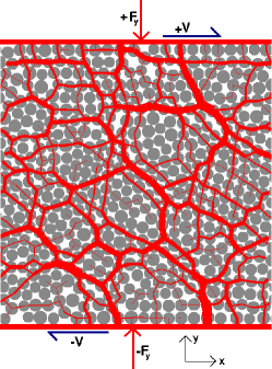
Figure 1: (color online) A polydisperse system of hard frictional disks in planar shear geometry with periodic boundary conditions in $x$ direction. A prescribed normal force $F_{y}$ to the confining walls, determines the constant external pressure of the system. The walls move with the same constant velocity $V$ in opposite directions. The width of the lines connecting the centers of contacting particles represents the magnitude of the normal contact forces above a threshold.

Results from different samples of various sizes are presented below. System sizes and simulation parameters are listed in Tab. 1.

Idx	$n$	$L_{y}$	$L_{x}$	$\sigma_{yy}$	$V$	$T_{\text{SS}}$	$T_{\text{Sim}}$
1	511	20	20	0.25	0.005-5.00	620	20000
2	1023	40	20	0.25	0.03-30.00	2500	10000
3	1023	40	20	0.0625	0.03-30.00	9900	10000
4	3199	50	50	0.25	0.01-30.00	4000	8000
5	2047	80	20	0.25	0.01-20.00	10000	4000-12000
6	3071	120	20	0.25	0.01-35.00	22000	6000
7	5119	200	20	0.25	0.01-30.00	64000	13000

Table 1: Parameters used in the simulations. $n$ is the number of disks in the sample. $T_{\text{SS}}$ denotes the characteristic time to approach steady state according to Eq. (17). $T_{\text{Sim}}$ is the total time simulated in each run.

As in Refs. Midi_04 ; daCruz_etal_05 ; Koval_etal_09 , the dimensionless inertial number, $I$, defined as a reduced form of shear rate $\dot{\gamma}$:

$$I=\dot{\gamma}\sqrt{\dfrac{m}{\sigma_{yy}}},$$ (1)

is used to characterize the state of the granular material in steady shear flow. In contrast to previous studies Midi_04 ; daCruz_etal_05 , the shear is not homogeneous in the present case (because of wall slip and of stronger gradients near the walls), and in general $\dot{\gamma}$ is different from $\dfrac{2V}{L_{y}}$. Thus, the shear rate has to be measured locally. We focus in the present study on shear localization at smooth walls and try to deduce constitutive laws in the boundary layer, associating the boundary layer behavior not only with wall slip, but also with the material behavior in a layer adjacent to the wall, the internal state of which might be affected by that of the bulk material.

II.2 System preparation

To preserve the symmetry of the top and the bottom walls, the system is horizontally filled. While distance $L_{y}$ between the walls is kept fixed, a third, vertical wall is introduced, on which the grains (which are temporarily rendered frictionless) settle in response to a “gravity” force field parallel to the $x$ axis. Then the force field is switched off, and the free surface of the material is smoothened and compressed by a piston transmitting $\sigma_{xx}=0.25$ (the same value as $\sigma_{yy}$ imposed in shear flow), until equilibrium is approached. System width $L_{x}$ is determined at this stage. Then the vertical wall and the piston are removed, the friction coefficients are attributed their final values $\mu_{\text{P}}$ and $\mu_{W}$ and periodic boundary conditions in the $x$ direction are enforced. With constant $L_{x}$ and variable $L_{y}$, the shearing starts with velocities $\pm V$ for the walls and an initial linear velocity profile within the granular layer.

II.3 Measured quantities

Before presenting the results, we first explain the method used to measure the effective friction coefficient, the velocity profiles and the inertial number. For a system in steady state, assuming a uniform stress tensor in the whole system, a common method to calculate the effective friction coefficient is to average the total tangential and normal forces acting on the walls over time and then calculate their ratio. Another way to calculate the effective friction coefficient is to consider the components of the stress tensor with its contact, kinetic and rotational contributions inside the system Moreau_97 ; Koval_etal_09 . The stress in our system is dominated by contact contributions. Let $\sigma_{\text{c}}^{i}$ denote the total contact stress tensor calculated for each particle $i$ with area $A_{i}{=}\pi d_{i}^{2}/4$:

$$\sigma_{\text{c}}^{i}=\dfrac{1}{A_{i}}\sum_{j\neq i}\vec{F_{ij}}\otimes\vec{r_{ij}}.$$ (2)

The summation runs over all particles $j$ having a contact with particle $i$. $\vec{F_{ij}}$ is the corresponding contact force and $\vec{r_{ij}}$ denotes the vector pointing from the center of particle $i$ to its contact point with particle $j$. We used both methods, but finding no significant difference, we present in all our corresponding graphs the effective friction coefficient ($\mu_{\text{eff}}$) measured in the interior of the system considering all terms of the stress tensor, although the contact contribution dominates.

Our calculation of the velocity profile accounts for particle rotations, which contribute to the local velocities averaged in stripes of thickness $\Delta y{=}1$ along the flow direction, as follows. To each horizontal stripe centered at $y{=}y^{\prime}$, we attribute a velocity by averaging the contributions of all the particles it contains (partly or completely) Laetzel_etal_00 :

$$\upsilon_{x}(y^{\prime})=\dfrac{\displaystyle\sum\limits_{i}\int\limits_{S_{i}}(\upsilon_{ix}+\omega_{i}r_{iy})dS}{\displaystyle\sum\limits_{i}S_{i}}.$$ (3)

$S_{i}$ denotes the surface fraction of particle $i$ within the stripe, $\upsilon_{ix}$ its center of mass velocity in $x$ direction, $\omega_{i}$ its angular velocity and $r_{iy}$ is the vertical distance between the center of mass of the particle and a differential stripe of vertical position $y$ and surface $dS$ within surface $S_{i}$. The velocity profiles presented here are also averaged over time intervals of $\Delta t{=}80$. Those time intervals follow each other directly without any gap.

In the calculation of the profiles of stress tensor, each particle contributes to each stripe in proportion to the surface area contained in the stripe. This corresponds to the scheme used in Laetzel_etal_00 and is slightly different from the coarse graining reviewed in Goldhirsch_10 in the sense that it is highly anisotropic (with a coarse graining scale of $L_{x}\times 1$) and does not incorporate the (stress free) regions beyond the walls. One other method is to split the contact contributions proportionally to their branch vector length within each stripe. One may also cut through the particles and add up the contact forces of all cut branch vectors. All three different methods lead to the same results in our simulations.

III Velocity profiles and strain localization

III.1 Steady state

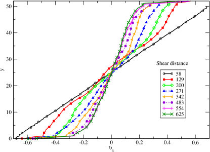
Figure 2: (color online) Transient to steady state for $V=0.70$ in a system with $L_{x}=50$ and $L_{y}=50$.

A system sheared with a certain constant velocity under prescribed normal stress is expected to reach a steady state after a transient. For instance, in a system of size $L_{x}{=}50$ and $L_{y}{=}50$ with a large shear velocity, $V{=}0.7$, the steady state is reached after a shear distance of about $\lambda\simeq 420$, corresponding to a shear strain of $\gamma\simeq 8$ (Fig. 2). The shear distance is calculated by multiplying the total shear velocity ($2V$) by time. Due to slip at the smooth walls and because of nonhomogeneous flow, the values attributed to the shear distance and the shear strain overestimate the real values in the bulk material. Transient times before steady state will be estimated in Sec. V.1, based on the constitutive laws.

In the steady state, the center of mass velocity in the system of Fig. 3 is not conserved, because of the constant velocity of the walls, and fluctuates about its vanishing average with an amplitude amounting to about $10\%$ of velocity $V$. This relatively high level of fluctuation, which is expected to regress in larger samples, reflects granular agitation within the sheared layer at large $V$. The fluctuations in height $L_{y}$ and solid fraction $\nu$ (measured in the whole system) amount to only about $1\%$ of the average after a short transient (Fig. 4). The initial sharp drop of $\nu$, for very small shear strains, is due to the combined effects of shear flow onset, friction activation and change of boudary conditions on the configuration prepared as described in Sec. II.2.

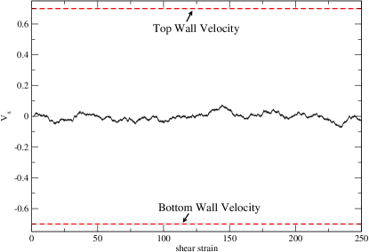
a) b)   

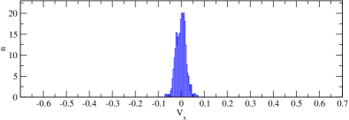
Figure 3: (color online) (a) Center of mass velocity versus shear strain for $V=0.70$ in a system with $L_{x}{=}50$ and $L_{y}{=}50$. The dashed red lines represent the velocity of the top and bottom walls. (b) Histogram of center of mass velocity (accumulated over a long time and over different simulated systems).

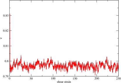
Figure 4: Solid fraction $\nu$ versus shear strain at $V{=}0.70$ in a system with $L_{x}{=}50$ and $L_{y}{=}50$.

In the steady state the profiles of the effective friction coefficient stay almost uniform throughout the system (Fig. 5), but fluctuate in time, which is a direct consequent of shearing with constant velocity and consequent fluctuations in the center of mass velocity.

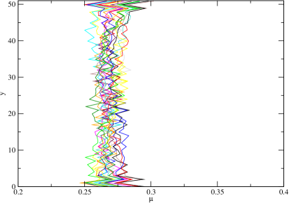
Figure 5: (color online) Profiles of the measured effective friction coefficient at different times in steady state for $V{=}0.70$ ($L_{x}{=}50$ and $L_{y}{=}50$).

III.2 Shear regimes and strain localization

a)
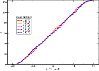
b)
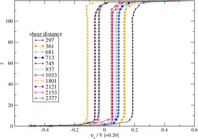
c)

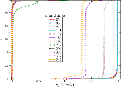
Figure 6: (color online) Velocity profiles at different shear distances for three different values of $V$, as indicated, in sample with height $L_{y}{=}120$ (System $6$ in Tab. 1).

Fig. 6 displays the time evolution of the velocity profiles of a system of initial height $L_{y}{=}120$ sheared with different velocities (a) $V{=}2.0$, (b) $V{=}0.2$ and (c) $V{=}0.03$. Those three cases are characteristics of three different regimes observed in different intervals as velocity $V$ decreases. At large velocity $V$, as for $V{=}2.0$ (panel (a) in Fig. 6), the velocity profile adopts (after a transient) a symmetric, almost linear shape with only small fluctuations in time. The shear rate is somewhat larger near the walls than in the bulk, but the latter region is homogeneously sheared. This is the fast or homogeneous shear regime (regime A in the sequel). For intermediate velocities, such as $V{=}0.2$ (panel (b) in Fig. 6) the shear rate is strongly localized at the walls, while, ten grain diameters away from the walls, the material is hardly sheared at all. While the profile shape is essentially stable, its position on the velocity axis fluctuates notably: the bulk material behaves like a solid block, but its velocity exhibits large fluctuations. To this situation we shall refer as the intermediate or two-shear band regime (regime B). Finally, for a low enough shear velocity, as for $V{=}0.03$ (panel (c) in Fig. 6) the profiles fluctuate very strongly and the top/bottom symmetry is broken. The shear strain strongly localizes at one wall, while the rest of the system, the bulk region and the opposite wall, moves like one single solid object Shojaaee_07 ; Shojaaee_etal_07 ; Shojaaee_etal_09 . This is the slow shear or one-shear band regime (regime C). Localization occasionally switches to the other wall, with a transition time that strongly depends on the system size and on the shear velocity (as we shall discuss in Sec. V.1).

In regime A the sheared layer behaves similarly to the observations reported by da Cruz et al. daCruz_etal_05 , in a numerical study of steady uniform shear flow of a granular material between rough walls. However, with rough walls the homogeneous shear regime persists down to very low velocities, in spite of increasing fluctuations. The smooth walls of our system, allowing for slip and rotation at the walls, are responsible for the more complex behavior Shojaaee_07 ; Shojaaee_etal_07 ; Shojaaee_etal_09 .

In order to be able to observe the three regimes, sample height $L_{y}$ should be large enough. In smaller systems ($L_{y}\,{\lesssim}\,80$) the effects of the boundary layers on the central region are strong enough to preclude the observation of a clearly developed intermediate regime. Sheared granular layers of smaller thickness most often exhibit a direct transition from regime A to regime C on decreasing velocity $V$.

Our system size analysis shows a discontinuous transition from regime B to regime C, at $V_{BC}{\simeq}0.10$ and a continuous transition between regimes A and B completed at $V_{AB}{\simeq}0.50$ Shojaaee_07 ; Shojaaee_etal_07 ; Shojaaee_etal_09 . $V_{BC}$ and $V_{AB}$ are system size independent.

Upon reducing the shear velocity in the intermediate shear regime towards $V_{BC}$ larger and larger fluctuations in the velocity fields are observed, involving increasingly long correlation times. Slightly above $V_{BC}$ the approach to a steady state becomes problematic, even after the largest simulated shear strain (or wall displacement) intervals. Then below $V_{BC}$ the width of the distribution of the bulk region velocities reaches its maximum value, $2V$, and the velocity profile stays for longer and longer time intervals in the localized state with one shear band at a wall (regime C). Such localized profiles can be regarded as quasi-steady states – as switches from one wall to the opposite one, ever rarer at lower velocities, sometimes occur. The lifetime of these one-shear band asymmetric steady shear profiles also increases with system height $L_{y}$, similar to ergodic time in magnetic systems Shojaaee_07 ; Shojaaee_etal_07 . These quasi-steady states also exhibit uniform stress profiles, contrary to the nonuniform ones in the transient states, as the localization pattern is switching to the other side (Fig. 7).

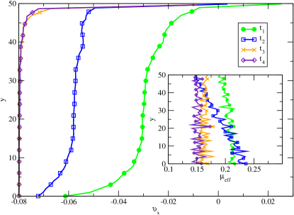
Figure 7: (color online) Profiles of velocity and effective friction coefficient (inset) in steady state and in the transient states for $V{=}0.08$ in a system with $L_{x}{=}50$ and $L_{y}{=}50$.

Fig. 8 (a) is a plot of center of mass velocity in the flow direction versus time in regime C. Most of the time, it is slightly fluctuating about the value of either one of the velocities of the walls, $\pm V$, as also illustrated in the histogram plot, Fig. 8 (b), for which values were accumulated over a long time and over different simulated systems. Transition times as the shear band switches directly from one wall to the other are measured as indicated. Those times are recorded to be discussed in Sec. V.1.2.

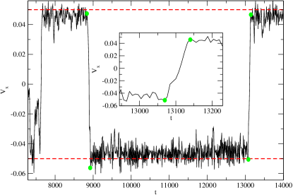
a) b)   

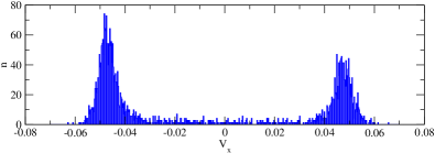
Figure 8: (color online) (a) Center of mass velocity fluctuations in steady state for $V{=}0.05$ in a system with $L_{x}{=}20$ and $L_{y}{=}20$. The dashed red lines represent the velocity of the top and bottom walls. The transition time (magnified in the inset) is measured at both ends of direct transitions from one wall to the other, between the round dots. (b) Histogram of center of mass velocities.

III.3 Slip velocity

The slip at smooth walls is a characteristic feature of the boundary region behavior.

To evaluate the slip velocity at the walls one needs to calculate the average of the surface velocity of particles in contact with the walls at their contact point. The slip velocity in this work is defined as the absolute value of the difference between the wall velocity and the average particle surface velocity at the corresponding wall, $\upsilon_{\text{0}}^{\text{slip}}$ at the bottom, respectively $\upsilon_{\text{L}_{y}}^{\text{slip}}$ at the top wall. To this end all particles in contact with the walls over the whole simulation time in steady state should be considered, and contribute

$$\upsilon_{\text{0}}^{\text{slip}}=V+\langle\upsilon_{ix}+\omega_{i}r_{i}\rangle_{i,t},$$ (4)

$$\upsilon_{\text{L}_{y}}^{\text{slip}}=V-\langle\upsilon_{ix}-\omega_{i}r_{i}\rangle_{i,t},$$ (5)

where $\upsilon_{ix}$ is the $x$ component of the center of mass velocity of particle $i$ of radius $r_{i}$ with angular velocity $\omega_{i}$.

Our observations show that the slip velocity in a certain shear velocity interval $0.2\,{\lesssim}\,V\,{\lesssim}\,1.0$ does not depend on the system size (Fig. 9). For larger shear velocities, though the general tendency is the same, slight deviations are observable. The apparent change of slope of the graph near $V{=}1$ could be associated with larger strain rates and inertial numbers in boundary layers, gradually approaching a collisional regime (see Sec. IV.3, about the coordination number).

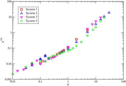
Figure 9: (color online) Slip velocity $\upsilon^{\text{slip}}$ (averaged over $\upsilon_{\text{0}}^{\text{slip}}$ and $\upsilon_{\text{L}_{y}}^{\text{slip}}$) measured as a function of shear velocity (systems specified in Tab. 1).

IV Constitutive laws

Constitutive laws were previously studied, in similar model materials, in homogeneous shear flow daCruz_etal_05 ; Hatano_07 ; Peyneau-Roux_08 . Their sensitivity to material parameters (restitution coefficients, friction coefficients and, possibly, finite contact stiffness) is reported, e.g. in RoCh11 . In our system we separate the boundary regions near both walls, from the central one (or bulk region). Unless otherwise specified, the boundary regions have thickness $h=10$. Near the walls, the internal state of the granular material is different, and we seek separate constitutive laws for the boundary layers and for the bulk material. While the bulk material is expected to abide by constitutive laws that apply locally, and should be the same as the ones identified in other geometries or with other boundary conditions daCruz_etal_05 ; Koval_etal_09 , the boundary constitutive law is expected to relate stresses to the global velocity variation across the layer adjacent to the wall. In a continuum description suitable for large scale problems, this will reduce to relating stresses to tangential velocity discontinuity.

IV.1 Constitutive laws in the bulk region

IV.1.1 Friction law

The steady state values of the inertial number ($I_{\text{bulk}}$) and that of the effective friction coefficient $\mu_{\text{eff}}$ are measured, as averages over time and over coordinate $y$ within the interval $h<y<L_{y}-h$. $\mu_{\text{eff}}$ is plotted as a function of $I_{\text{bulk}}$ for all different system sizes in Fig. 10, showing data collapse for different sample sizes.

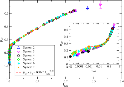
Figure 10: (color online) $\mu_{\text{eff}}$ as a function of inertial number in the bulk region for different system sizes (see Tab. 1). The fit function is calculated according to Eq. 6 for $\mu_{0}{=}0.25$. The error bars are much smaller than the symbols. The inset is a semilogarithmic plot of the same data.

The apparent influence of the choice of $h$ on the measured effective friction coefficient and inertial number in the bulk region is presented in Fig. 11 for two different system sizes and for two different $h$ values.

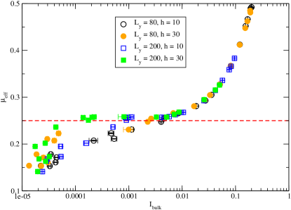
Figure 11: (color online) Influence of $h$ on $\mu_{\text{eff}}$ as a function of inertial number in the bulk region (data from systems $5$ and $7$ in Tab. 1). The dashed red line represents the critical friction coefficient $\mu_{0}{=}0.25$.

We observe that some data points with finite values of $I_{\text{bulk}}$ ($I_{\text{bulk}}>10^{-4}$) are shifted to much smaller values of $I_{\text{bulk}}$ upon increasing $h$: compare the open and full symbols in Fig. 11. This effect is apparent in regimes B and C. It is due to the creep phenomenon (as was also observed in the annular shear cell in Koval_etal_09 ), which causes some amount of shearing at the edges of the bulk region, adjacent to the boundary layer, although the effective friction coefficient is below the critical value. Although the local shear stress is too small for the material to be continuously sheared, the ambient noise level, due to the proximity of the sheared boundary layer, entails slow rearrangements that produce macroscopic shear Unger_10 . Upon increasing $h$ the central bulk region excludes the outer zone that is affected by this creep effect. The critical friction coefficient, from Fig. 11, is $\mu_{0}{=}0.25$ (below which the data points are sensitive to the value of $h$), which is consistent with the results of the literature daCruz_etal_05 ; Koval_etal_09 .

Fitting $\mu_{\text{eff}}-\mu_{0}$ with a power law function, as in Hatano_07 ; Peyneau-Roux_08

$$\mu_{\text{eff}}-\mu_{0}=A\cdot I_{\text{bulk}}^{B},$$ (6)

the following coefficient values yield good results (see Fig. 10):

$$\mu_{0}=0.24\pm 0.01,$$

$$A=0.92\pm 0.05,$$

$$B=0.80\pm 0.05.$$

IV.1.2 Dilatancy law

We now focus on the variation of solid fraction $\nu$ as a function of inertial number within the bulk region. $\nu$ is averaged over time, once a steady state is achieved, within the central region, $h<y<L_{y}-h$. Function $\nu_{\text{bulk}}(I_{\text{bulk}})$ is plotted in Fig. 12 for different system sizes, leading once again to a good data collapse. A linear fit for all data sets in the interval $0.03<I_{\text{bulk}}<0.20$ gives:

$$\nu_{\text{bulk}}=0.81-0.30\cdot I_{\text{bulk}},$$ (7)

which is consistent with the linear fit in daCruz_etal_05 ; Koval_etal_09 .

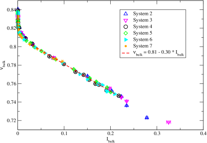
Figure 12: (color online) $\nu$ as a function of inertial number in the bulk region. The error bars plotted are much smaller than the symbols (systems specified in Tab. 1).

IV.2 Constitutive laws in the boundary layer

In order to characterize the state of the boundary layer of width $h$ adjacent to the wall (recall $h=10$ by default), we use a local inertial number $I_{\text{boundary}}$, defined as follows:

$$I_{\text{boundary}}^{\text{top/bottom}}=\sqrt{\dfrac{m}{\sigma_{yy}}}\times\left<\dfrac{\Delta\upsilon^{\text{top/bottom}}}{h}\right>_{t},$$ (8)

with

$$\Delta\upsilon^{\text{top}}=V-\upsilon_{x}(L_{y}-h),$$ (9)

$$\Delta\upsilon^{\text{bottom}}=\upsilon_{x}(h)+V.$$

IV.2.1 Friction law

Fig. 13 is a plot of $\mu_{\text{eff}}$ as a function of the inertial number $I_{\text{boundary}}$ in the boundary layer for all different system sizes.

In steady state the value of $\mu_{\text{eff}}$ in the boundary layer has to be equal to the averaged one in the bulk. The observed shear increase (in regime A) or localization (in regimes B and C) near the smooth walls entails larger values of inertial numbers in the boundary region. An equal value of $\mu_{\text{eff}}$ in the bulk and in the boundary zone then requires that the graph of function $\mu_{\text{eff}}(I_{\text{boundary}})$ is below its bulk counterpart in the inertial number interval measured.

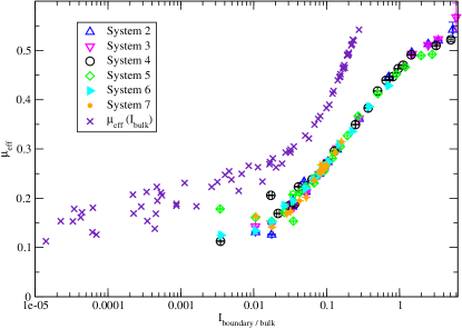
Figure 13: (color online) $\mu_{\text{eff}}$ as a function of inertial number in the boundary layer. The error bars plotted are much smaller than the symbols. As $I_{\text{boundary}}{>}I_{\text{bulk}}$ (shear localization at smooth walls) $\mu_{\text{eff}}(I_{\text{boundary}})$ lies always beneath $\mu_{\text{eff}}(I_{\text{bulk}})$. The presented $\mu_{\text{eff}}(I_{\text{bulk}})$ curve is based on the same data set as Fig. 10.

In Sec. IV.1 we have seen that the friction law can be identified in the bulk independently of $h$ (see Fig. 11), as an intrinsic constitutive law. According to the definition of $I_{\text{boundary}}$ in Eqs. (8) and (9) any constitutive relation involving $I_{\text{boundary}}$ should trivially depend on $h$. In shear regimes B and C, there is no shearing in the bulk region, and consequently $\Delta\upsilon$ in the numerator of Eq. (8) does not change with $h$. On multiplying the measured $I_{\text{boundary}}$ with the corresponding value of $h$, we thus expect the data points belonging to shear regimes B and C to coincide (Fig. 14). In regime A, in contrast, the existence of shear in the bulk region leads to an apparent $h$ dependence of the measured $\Delta\upsilon$. Accordingly, after multiplying $I_{\text{boundary}}$ with $h$, the curves do not merge. The critical effective friction coefficient at which the deviation of the curves begins corresponds to $\mu_{0}{=}0.25$ (the dashed horizontal line in Fig. 14), in agreement with the results in Sec. IV.1.1. This makes it more difficult to identify a constitutive law for the boundary layer, when the bulk region is sheared in regime A.

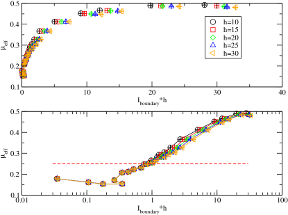
Figure 14: (color online) $\mu_{\text{eff}}$ versus $h\times I_{\text{boundary}}$ on linear (top panel) and semi-logarithmic (bottom panel) plots. The dashed horizontal line indicates the critical state value $\mu_{\text{eff}}=\mu_{0}{=}0.25$.

The behavior of $\mu_{\text{eff}}$ shown in Fig. 14 is apparently anomalous in two respects: $(i)$ the $\Delta\upsilon$ dependence of $\mu_{\text{eff}}$ does not seem to follow a single curve (suggesting $\mu_{\text{eff}}$ depends on other state parameters than the velocity variation across the boundary zone); $(ii)$ $\mu_{\text{eff}}$ is a decreasing function of $I_{\text{boundary}}$ for the first data points, as $h\times I_{\text{boundary}}<0.2$. In Fig. 15 (a), we take a closer look at the low $I_{\text{boundary}}$ data points, which bear number labels 1 to 6 in the order of increasing shear velocity $V$. The transition from regime C (one shear band) to regime B (two shear bands) occurs between points 4 and 5, whence a decrease in $I_{\text{boundary}}$, as the velocity change across the sheared boundary layers changes from $2V$ to merely $V$. In an attempt to identify one possible other variable influencing boundary layer friction, the symbols on Fig. 15 (a) also encode the value of the bulk density. We note then that points 4 and 6, which have different friction levels, although approximately the same $I_{\text{boundary}}$, correspond to different bulk densities. The constitutive laws in the boundary layer might thus depend on parameter $\nu_{\text{bulk}}$ in addition to $I_{\text{boundary}}$.

a)  
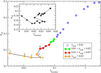
b)

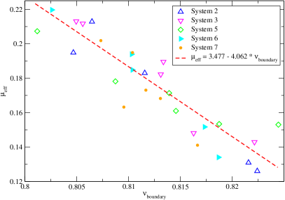
Figure 15: (color online) (a) $\mu_{\text{eff}}$ as a function of $I_{\text{boundary}}$ (data from system $5$).The full symbols belong to the states with bulk densities larger than the critical value $\nu_{c}{=}0.81$ (see Eq. (7)). The full diamonds have a density between $0.81$ and $0.82$, full squares have a density between $0.82$ and $0.83$ and full circles have a density larger than $0.83$. The inset represents the zig-zag with some more data points, which are absent in the master graph for the sake of clarity. (b) $\mu_{\text{eff}}$ as a function of $\nu_{\text{boundary}}$. The error bars are smaller than the symbols.

As to issue $(ii)$, the decrease of $\mu_{\text{eff}}$ before the zig-zag pattern on the curve of Fig. 15 (a) (data points $1$ to $3$) is associated to an increase in the boundary layer density with $I_{\text{boundary}}$. This is not the case in all of the systems and these features strongly depend on the preparation and the initial packing density (compaction in the absence of friction). Independent of whether $\mu_{\text{eff}}$ in regime C increases or not as $I_{\text{boundary}}$ increases, $\mu_{\text{eff}}$ always displays a decreasing tendency as $\nu_{\text{boundary}}$ increases, just like $\mu_{\text{eff}}$ and $\nu$ vary in opposite directions in bulk systems under controlled normal stress, as shown in Ref. daCruz_etal_05 , or as expressed by Eqs. (6) and (7) (panel (b) in Fig. 15). The lack of a perfect collapse of the data points around the decreasing linear fit of Fig. 15 (b) shows however that the state of the boundary layer in slowly sheared systems does not depend on a single local variable, but is influenced by the state of the neighboring bulk material, as remarked above.

IV.2.2 Dilatancy law

After averaging the profiles of solid fraction and inertial number over the whole simulation time in steady state in the boundary region, $\nu_{\text{boundary}}(I_{\text{boundary}})$ graphs are then plotted in Fig. 16 (a) for different system sizes. In Fig. 16 (b), $\nu_{\text{bulk}}(I_{\text{bulk}})$ and $\nu_{\text{boundary}}(I_{\text{boundary}})$ are compared for all data sets. $\nu_{\text{boundary}}$ and $\nu_{\text{bulk}}$ drop proportionally with increasing $I_{\text{bulk}}$ (shear velocity) until $I_{\text{bulk}}{\simeq}0.08$ (in shear regime A). Afterwards, the drop in $\nu_{\text{boundary}}$ is much steeper (Fig. 16 (c)).

a)
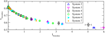
b)
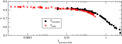
c)   

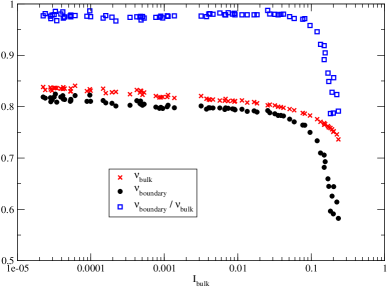
Figure 16: (color online) (a) $\nu$ as a function of inertial number in the boundary layers (systems specified in Tab. 1). (b) $\nu_{\text{boundary}}(I_{\text{boundary}})$ compared to $\nu_{\text{bulk}}(I_{\text{bulk}})$. (c) The ratio between $\nu_{\text{boundary}}$ and $\nu_{\text{bulk}}$ as a function of $I_{\text{bulk}}$.

IV.3 Coordination number

The coordination number (average number of contacts per grain) is a quantitative measure of the status of the contact network. Fig. 17 shows the measured coordination number in the bulk and in the boundary layers as a function of inertial numbers in these two regions. The data are collected from different systems in Tab. 1.

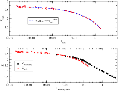
Figure 17: (color online) Coordination number as a function of inertial number in the bulk and boundary regions. The error bars are much smaller than the symbols.

The bulk coordination number, $Z_{\text{bulk}}$ is fitted with the power law function $Z_{\text{bulk}}=2.70-2.76\cdot I_{\text{bulk}}^{0.44}$. The boundary region coordination number, $Z_{\text{boundary}}$, follows a slightly different dependency on $I_{\text{boundary}}$, which becomes noticeable for $I_{\text{boundary}}\,{\gtrsim}\,0.1$, which corresponds to $V{\simeq}1$ (see Sec.III.3). It drops to smaller values, as $I_{\text{boundary}}$ reaches larger values, above 1. The decrease of coordination number as a function of inertial number is compatible with the observations of daCruz_etal_05 , in which some effect of restitution coefficient on $Z$ was however reported. The finite softness of the particles is also known to affect coordination numbers Silbert_etal_01 much more than the rheological laws. It is only for configurations extremely close to equilibrium that coordination numbers are observed to exceed the minimum value 3 for stable packings of frictionless disks (excluding rattlers), and even in quite slow flows this condition is not fulfilled.

V Applications

We now exploit the constitutive relations and other observations reported in the previous sections to try and deduce some features of the global behavior of granular samples sheared between smooth walls.

V.1 Transient time

V.1.1 Transient to steady state in regime A

The bulk friction law of Sec. IV.1.1 can be used to evaluate the time for a system to reach a uniform shear rate in regime A, if we assume constant and uniform solid fraction $\nu$ and normal stress $\sigma_{yy}$, and velocities parallel to the walls at all times. We write down the following momentum balance equation:

$$\dfrac{\partial(\rho\nu\upsilon_{x})}{\partial t}=\dfrac{\partial\sigma_{xy}}{\partial y},$$ (10)

looking for the steady solution: $\upsilon_{x}=\dot{\gamma}y$. Assuming constant $\rho$, $\nu$ and $\sigma_{yy}$ we can write:

$$\rho\nu\dfrac{\partial\upsilon_{x}}{\partial t}=\dfrac{\partial}{\partial y}\left[\mu_{\text{eff}}(\dot{\gamma})\right]\sigma_{yy},$$ (11)

which leads by derivation to:

$$\rho\nu\dfrac{\partial\dot{\gamma}}{\partial t}=\dfrac{\partial^{2}}{\partial y^{2}}\left[\mu_{\text{eff}}(\dot{\gamma})-\mu_{0}\right]\sigma_{yy}.$$ (12)

Separating the shear rate field into a uniform part $\dot{\gamma}_{0}$ and a $y$-dependent increment $\Delta\dot{\gamma}$, and assuming as an approximation just a linear dependency of $\mu_{\text{eff}}$ on $\dot{\gamma}$, we can rewrite Eq. (12) as follows:

$$\rho\nu\dfrac{\partial\Delta\dot{\gamma}}{\partial t}=\sigma_{yy}\dfrac{\partial\mu_{\text{eff}}}{\partial\dot{\gamma}}\dfrac{\partial^{2}}{\partial y^{2}}\Delta\dot{\gamma},$$ (13)

which is a diffusion equation with diffusion coefficient

$$D=\frac{\partial\mu_{\text{eff}}}{\partial\dot{\gamma}}\frac{\sigma_{yy}}{\rho\nu}.$$ (14)

The characteristic time to establish the steady state profile (uniform $\dot{\gamma}$ over the whole sample height $L_{y}$) is then:

$$T_{\text{SS}}=\dfrac{L_{y}^{2}}{D}.$$ (15)

A linear fit of function $\mu_{\text{eff}}(I_{\text{bulk}})$ (see Fig. 10) in interval ($0.03<I_{\text{bulk}}<0.20$) is:

$$\mu_{\text{eff}}=0.27+1.16\cdot I_{\text{bulk}}.$$ (16)

According to Eqs. (1), (14), (15) and (16) this leads to:

$$T_{\text{SS}}\simeq 1.56L_{y}^{2}.$$ (17)

The estimated values $T_{\text{SS}}$ for different system sizes is listed in Tab. 1. As $T_{\text{SS}}$ grows like $L_{y}^{2}$, very long simulation runs become necessary to achieve steady states in tall (large $L_{y}$) samples, and some unstable, but rather persistent, distributions of shear rate can be observed Aharonov_Sparks_02 ; Peyneau-Roux_08 . Our data for $L_{y}{=}120$ and $L_{y}{=}200$ may still pertain to slowly evolving profiles, even though the constitutive law can be measured in approximately homogeneous regions of the sheared layer over time intervals in which profile changes are negligible.

V.1.2 Transition from one wall to the other in regime C

As stated in Sec. III.2 in regime C the asymmetric velocity profiles can be regarded as steady states and the switching stages in which the shear band changes sides are transient states in which the shear stress is not uniform through the granular layer. We now try to estimate the characteristic time for such transitions. This estimation does not rely on a specific model for the triggering mechanism of the transition. It is based on the simple idea that the transition takes place when the solid block is accelerated due to a shear stress difference between the top and the bottom boundary zones. Taking the whole bulk region as a block of mass $M$ moving with the velocity of the top wall $V$, a transition to velocity $-V$ with acceleration $A$ will take:

$$T_{\text{transition}}=\dfrac{2V}{A},$$ (18)

in which the acceleration $A$ is equal to:

$$A=\dfrac{(\sigma_{xy}^{top}-\sigma_{xy}^{bottom})L_{x}}{M}.$$ (19)

Substituting $M{=}\rho\nu L_{x}L_{y}$ and $\sigma_{xy}^{top}-\sigma_{xy}^{bottom}{=}\Delta\mu\sigma_{yy}$ with $\Delta\mu{=}\mu^{top}-\mu^{bottom}$ one gets:

$$T_{\text{transition}}=\dfrac{2\rho\nu VL_{y}}{\Delta\mu\sigma_{yy}}.$$ (20)

Accordingly, the transition time increases proportionally to the shear velocity and to system height $L_{y}$. Using $\nu\simeq 0.84$, $\sigma_{yy}=0.25$ and taking $\Delta\mu\simeq 0.05$ as a plausible value in shear regime C (see Figs.  7 and 14) we calculate $\frac{T_{\text{transition}}}{V}$ as a function of system height $L_{y}$. In Fig. 18 these estimated times are compared to transition times that are measured as explained in the caption of Fig. 8.

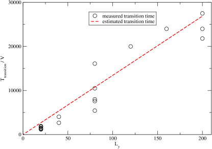
Figure 18: (color online) Transition time divided by the shear velocity as a function of system height. Empty circles correspond to measured times, while the (red) dashed line plots estimated ones, using (20).

Admittedly, one does not observe only direct, sharp transitions in which localization changes from one wall to the opposite one. Some transient states are more uncertain and fluctuating, and the system occasionally returns to a localized state on the same wall after some velocity gradient has temporarily propagated within the central region. The data points of Fig. 18 correspond to the well-defined transitions, which become less frequent with increasing system height. Thus a unique data point was recorded for systems with $L_{y}=120$ and $L_{y}=160$. The comparison between estimated and measured transition times is encouraging, although the value of $\Delta\mu$ in (20) is of course merely indicative (it is likely to vary during the transition), and the origin of such asymmetries between walls is not clear.

V.2 Transition velocity $V_{AB}$

$\mu_{0}{=}0.25$ from the power law fit in Eq. (6) corresponds to the minimal value of the bulk effective friction coefficient, the critical value below which the granular material cannot be continuously sheared (except for local creep effects in the immediate vicinity of an agitated layer).

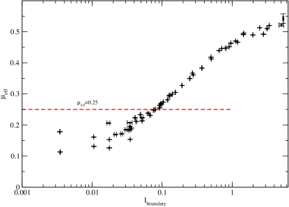
Figure 19: (color online) The critical $I_{\text{boundary}}$, which corresponds to $\mu_{0}{=}0.250$ (dashed red line) and determines the the critical velocity $V_{AB}$ for the transition from regime A to regime B.

Fig. 19 gives the value of the inertial number in the boundary region, such that the boundary friction coefficient matches $\mu_{0}{=}0.25$:

$$\mu_{0}=0.25\Rightarrow I_{\text{boundary}}{=}0.086\pm 0.005.$$ (21)

Thus for $I_{\text{boundary}}\,{\lesssim}\,0.086$ we expect no shearing in the bulk. According to Eqs. (8) and (9) this results in $V{=}0.485\pm 0.028$, in very good agreement with our observations reported in Sec. III.2 ($V_{AB}\simeq 0.50$).

The explanation of the transition from regime A to regime B is simple: the boundary layer, with a smooth, frictional wall, has a lower shear strength (as expressed by a friction coefficient) than the bulk material. Thus for uniform values of stresses $\sigma_{yy}$ and $\sigma_{xy}$ in the sample, such that their ratio $\sigma_{xy}/\sigma_{yy}$ is comprised between the static friction coefficient of the bulk material and that of the boundary layers, shear flow is confined to the latter.

V.3 Transition to regime C at velocity $V_{BC}$

Although it is not systematically observed, and is likely to depend on the bulk density, the decreasing trend of $\mu_{\text{eff}}$ in the boundary layer as a function of $\Delta\upsilon$ or of $I_{\text{boundary}}$, as apparent in Figs. 14 and 15 (a), provides a tempting explanation to the transition from regime B to regime C. Assuming $\mu_{\text{eff}}$  for given, constant $\sigma_{yy}$, to vary in the boundary layers as

$$\mu_{\text{eff}}=\mu_{0}-\alpha|\Delta\upsilon|,\ \ \mbox{with}\ \alpha>0,$$ (22)

one may straightforwardly show that the symmetric solution with $\Delta\upsilon=\pm V$, and solid bulk velocity $\upsilon_{s}=0$, is unstable. A simple calculation similar to the one of Sec. V.1.2 shows that velocity $\upsilon_{s}$, if it differs from zero by a small quantity $\delta\upsilon_{s}$ at $t=0$, will grow exponentially,

$$\upsilon_{s}(t)=\delta\upsilon_{s}\exp\frac{2\alpha L_{x}\sigma_{yy}t}{M},$$ (23)

until it reaches $\pm V$, with the sign of the initial perturbation $\delta\upsilon_{s}$. Transition velocity $V_{BC}$ would then be associated to a range of velocity differences $\Delta\upsilon$ across the boundary layer with softening behavior (i.e., decreasing function $\mu_{\text{eff}}(I_{\text{boundary}})$).

In view of Fig. 15 (a), where the BC transition takes place at point 4, this seems plausible, as the slope of function $\mu_{\text{eff}}(I_{\text{boundary}})$ appears to vanish towards this point.

VI Conclusion

In this work we have investigated shear localization at smooth frictional walls in a dense sheared layer of a model granular material. The slip at the walls induces inhomogeneities in the system leading to three different shear regimes. As the wall velocity is reduced from large values, two transitions successively occur, in which shear deformation localizes, first symmetrically near opposite walls, and then at a single wall. Measuring stress tensor, inertial number and solid fraction locally in the whole system, the constitutive laws have been identified in the bulk (for which our results agree with the published literature) and in the boundary layer. Those constitutive laws, supplemented by an elementary stability analysis, allow us to predict the occurrence of both transitions, as well as characteristic transient times. The consistence of the derived constitutive laws for the bulk rheology with those in previous contributions daCruz_etal_05 using the MD method, confirm that the rheology is the same for CD and for MD in the limit of large contact stiffness.

Additional numerical work should be carried out in order to assess the dependence of the boundary layer constitutive law on the state of the adjacent bulk material with full generality. The application of similar constitutive laws for smooth boundaries should be attempted in a variety of flow configurations: inclined planes, vertical chutes, circular cells. Finally, the success of the simple type of stability analysis carried out in the present work calls for more accurate, full-fledged approaches in which couplings of shear stress and deformation with the density field would be taken into account.

- (1) C. S. Campbell. Granular material flows – an overview. Powder Technology, 162:208–229, 2006.
- (2) Y. Forterre and O. Pouliquen. Flows of dense granular material. Annual Review of Fluid Mechanics, 40:1–24, 2008.
- (3) F. da Cruz, S. Emam, M. Prochnow, J.-N. Roux, and F. Chevoir. Rheophysics of dense granular materials: Discrete simulation of plane shear flows. Physical Review E, 72:021309, 2005.
- (4) GDR Midi. On dense granular flows. The European Physical Journal E, 14(4):341–365, 2004.
- (5) G. Koval, J.-N. Roux, A. Corfdir, and F. Chevoir. Annular shear of cohesionless granular materials: From the inertial to quasistatic regime. Physical Review E, 79(2):021306, 2009.
- (6) L. Lacaze and R. R. Kerswell. Axisymmetric granular collapse: A transient 3d flow test of viscoplasticity. Phys. Rev. Lett., 102:108305, 2009.
- (7) P. Jop, Y. Forterre, and O. Pouliquen. A constitutive law for dense granular flows. Nature, 441:727, 2006.
- (8) S. B. Savage and M. Sayed. Stresses developed by dry cohesionless granular materials sheared in an annular shear cell. Journal of Fluid Mechanics, 142:391–430, 1984.
- (9) D. M. Hanes and D. L. Inman. Observations of rapidly flowing granular-fluid materials. Journal of Fluid Mechanics, 150:357–380, 1985.
- (10) O. Pouliquen. Scaling laws in granular flows down rough inclined planes. Physics of Fluids, 11(3):542, 1999.
- (11) L. E. Silbert, D. Ertas, G. S. Grest, T. C. Halsey, D. Levine, and S. J. Plimpton. Granular flow down an inclined plane: Bagnold scaling and rheology. Physical Review E, 64(5):051302, 2001.
- (12) G. Lois, A. Lemaître, and J. M. Carlson. Numerical tests of constitutive laws for dense granular flows. Physical Review E, 72(5):051303, 2005.
- (13) N. Taberlet, P. Richard, and R. Delannay. The effect of sidewall friction on dense granular flows. Computers and Mathematics with Applications, 55(2):230–234, 2008.
- (14) R. M. Nedderman. Statics and kinematics of granular materials. Cambridge University Press, Cambridge, 1992.
- (15) R. Artoni, A. Santomaso, and P. Canu. Effective boundary conditions for dense granular flows. Physical Review E, 79(3):031304, 2009.
- (16) X. M. Zheng and J. M. Hill. Molecular dynamics simulation of granular flows: Slip along rough inclined planes. Computational Mechanics, 22(2):160–166, 1998.
- (17) M. Y. Louge. computer simulations of rapid granular flows of spheres interacting with a flat, frictional boundary. Physics of Fluids, 6(7):2253–2269, 1994.
- (18) Z. Shojaaee, L. Brendel, J. Török, and D.E. Wolf. Shear flow of dense granular materials near smooth walls. II. block formation and suppression of slip by rolling friction, 2012.
- (19) Z. Shojaaee. Phasenübergangsmerkmale der Rheologie granularer Materie. Diploma thesis, University of Duisburg-Essen, Duisburg, Germany, 2007.
- (20) Z. Shojaaee, L. Brendel, and D. E. Wolf. Rheological transition in granular media. In C. Appert-Rolland, F. Chevoir, P. Gondret, S. Lassarre, J-P. Lebacque, and M. Schreckenberg, editors, Traffic and Granular Flow, pages 653–658, Berlin, 2009. Springer.
- (21) Z. Shojaaee, A. Ries, L. Brendel, and D. E. Wolf. Rheological transitions in two- and three-dimensional granular media. In M. Nakagawa and S. Luding, editors, Powders and Grains, pages 519–522, New York, 2009. American Institute of Physics.
- (22) J.J. Moreau and P.D. Panagiotopoulos. Nonsmooth Mechanics and Applications. Springer, Vienna, 1988.
- (23) M. Jean. The non-smooth contact dynamics method. Comput. Methods Appl. Mech. Engrg., 177(3):235–257, 1999.
- (24) L. Brendel, T. Unger, and D. E. Wolf. Contact Dynamics for Beginners. In H. Hinrichsen and D. E. Wolf, editors, The Physics of Granular Media, chapter 14, pages 325–343. Wiley-VCH, Berlin, 2004.
- (25) F. Radjai and V. Richefeu. Contact dynamics as a nonsmooth discrete element method. Mechanics of Materials, 41(6):715–728, 2009.
- (26) J. J. Moreau. Numerical investigation of shear zones in granular materials. In D. E. Wolf and P. Grassberger, editors, Friction, Arching, Contact Dynamics, pages 233–247. World Scientific, London, 1997.
- (27) M. Lätzel, S. Luding, and H. J. Herrmann. Macroscopic material properties from quasi-static, microscopic simulations of a two-dimensional shear-cell. Granular Matter, 2(3):123–135, 2000.
- (28) I. Goldhirsch. Stress, stress asymmetry and couple stress: from discrete particles to continuous fields. Granular Matter, 12(3):239–252, 2010.
- (29) T. Hatano. Power-law friction in closely packed granular materials. Physical Review E, 75:060301(R), 2007.
- (30) P. E. Peyneau and J.-N. Roux. Frictionless bead packs have macroscopic friction, but no dilatancy. Physical Review E, 78(1):011307, 2008.
- (31) J.-N. Roux and F. Chevoir. Dimensional Analysis and Control Parameters. In F. Radjaï and F. Dubois, editors, Discrete-element Modeling of Granular Materials, chapter 8, pages 199–232. ISTE-Wiley, 2011.
- (32) T. Unger. Collective rheology in quasi static shear flow of granular media. arXiv:1009.3878v1.
- (33) E. Aharonov and D. Sparks. Shear profiles and localization in simulations of granular materials. Physical Review E, 65:051302, 2002.