Origin and Use of the Laplace Distribution in Daily Sunspot Numbers

Abstract

Recently Pop (Solar Phys. 276, 351, 2012) identified a Laplace (or double exponential) distribution in the number of days with a given absolute value in the change over a day, in sunspot number, for days on which the sunspot number does change. We show this phenomenological rule has a physical origin attributable to sunspot formation, evolution, and decay, rather than being due to the changes in sunspot number caused by groups rotating onto and off the visible disc. We also demonstrate a simple method to simulate daily sunspot numbers over a solar cycle using the Pop (2012) result, together with a model for the cycle variation in the mean sunspot number. The procedure is applied to three recent solar cycles. We check that the simulated sunspot numbers reproduce the observed distribution of daily changes over those cycles.

1 Introduction

Section:Introduction

Sunspots have been studied scientifically since the invention of the telescope, and reliable daily sunspot number records are available from the early 1800s. The accepted quantity to characterise solar activity is the international sunspot number

$$\ilabel{eq:issn}s=k(10g+n),$$ (1)

where $n$ is the number of individual sunspots, $g$ is the number of sunspot groups, and $k$ is a correction factor (Bruzek and Durrant, 1977). The sunspot number changes in a secular or long-term fashion with the semi-regular 11-year sunspot cycle, driven by an internal magnetic dynamo which generates the magnetic field (Tobias, 2002). The secular change in sunspot number exhibits apparent randomness, as evidenced by the extensive literature describing the smoothed daily sunspot number (typically a monthly average) as a stochastic, or chaotic time series. In particular, the peak and timing of the different solar cycles shows considerable variation (Petrovay, 2010).

Sunspot numbers also vary on shorter time scales, in particular daily, as a result of the complicated local processes associated with sunspot formation, evolution, and decay. The short-timescale variation produces large excursions in sunspot number, up to 100 per day in extreme cases (Noble and Wheatland, 2011). The large day to day variations are caused by the rapid evolution of magnetic structures, and the sudden appearance/disappearance of large active regions. These rapid developments can have important consequences for the space weather experienced on Earth (Committee on the Societal and Economic Impacts of Severe Space Weather Events, 2008).

Recently, it was demonstrated that the change $\Delta s$ in the daily sunspot number (for days on which the number does change) follows a Laplace, or double exponential distribution (Pop, 2012). Including the case of days with no changes, Pop (2012) modelled the distribution $f(\Delta s)$ of the change in sunspot number with the functional form

$$\ilabel{eq:pop_{l}aw}f(\Delta s)=A\mathbb{I}(\Delta s<0)\exp(\Delta s/B)+A\mathbb{I}(\Delta s>0)\exp(-\Delta s/B)+C\delta(\Delta s),$$ (2)

where $A,\,B$, and $C$ are constants, and where $\mathbb{I}(x)$ is the indicator function defined by $\mathbb{I}(x)=1$ for $x$ true, and $\mathbb{I}(x)=0$ for $x$ false. The parameter $C$ determines the fraction of zero changes, and $B$ is the mean absolute change for days on which the number does change. Normalisation of Equation (eq:pop_law) requires $A=(1-C)/2B$.

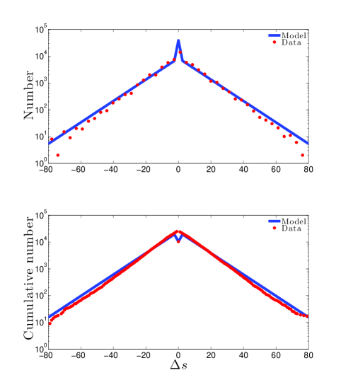
Figure fig:f1 shows the observed distribution for the daily sunspot number using the NGDC data for 1850–2011, and illustrates the exponential form identified by Pop (2012). The top panel is a histogram of daily changes $\Delta s$. The bottom panel shows the cumulative number of changes greater than $\Delta s_{i}$, for positive changes:

$$N(\Delta s\geq\Delta s_{i})=\sum_{i}\mathbb{I}(\Delta s\geq\Delta s_{i}>0),$$ (3)

and the cumulative number less than $\Delta s_{i}$ for negative changes:

$$N(\Delta s\leq\Delta s_{i})=\sum_{i}\mathbb{I}(\Delta s\leq\Delta s_{i}<0).$$ (4)

Both panels use a logarithmic scaling on the vertical axis. The red dots in the panels show the data, and the blue curves show the model distribution defined by Equation (eq:pop_law), with parameters $B$ and $C$ estimated from the data using maximum likelihood (Eliason, 1993). The adherence to the exponential form in Figure fig:f1 is striking. There are a large number of days with no change in sunspot number, and Pop (2012) refers to $\Delta s=0$ as a “special state”. The distribution is remarkably symmetric about $\Delta s=0$. Pop (2012) also investigated the solar cycle dependence of the observed distribution, and found that the exponential rule in absolute changes is most closely adhered to over whole cycles, with the greatest departure near minima of cycles.

It is surprising that the Laplace distribution in the change in daily sunspot number was not identified and discussed in the literature earlier. The behaviour was previously noted in smoothed data (Lepreti, Kossobokov, and Carbone, 2009), and an approximate exponential dependence in the distribution of overall sunspot numbers, related to Equation (eq:pop_law), was also commented on Noble and Wheatland (2011). However, Pop (2012) showed that the adherence of the observed changes in daily sunspot number to the Laplace distribution defined by Equation (eq:pop_law) is much stricter than the approximate exponential distribution of overall sunspot number. The Laplace distribution (Equation (eq:pop_law)) represents a newly identified phenomenological rule describing the way in which the daily sunspot number varies, which should have application for modelling and prediction. The origin of the distribution is not obvious. Changes in sunspot number occur daily due to sunspot group formation, evolution and decay, the appearance/disappearance of spots and spot splitting (referred to here as spot evolution), and also due to sunspot groups and individual spots rotating onto and off the visible disc. If the law is due to spot and group evolution, then the phenomenological rule must have a physical origin.

In this paper we demonstrate that the Laplace distribution of changes in sunspot number is caused by sunspots forming, evolving, and decaying, and is not a result of rotation on and off the disc. We then also present a simple Monte Carlo method, based on Equation (eq:pop_law) and some additional assumptions, for simulating sunspot numbers over solar cycles.

2 Origin of the Laplace Distribution

Section1 To investigate the origin of the observed distribution in changes in sunspot number we use reports of sunspot groups on the Sun, for 1981-2011, compiled by US National Oceanic and Atmospheric Administration (USAF/NOAA). The daily change in sunspot number

$$\ilabel{eq:changeins}\Delta s=k\left(10\Delta g+\Delta n\right)$$ (5)

can be decomposed into changes due to rotation of regions and spots onto and off the disc $\Delta s_{\rm r}$, and changes due to group and sunspot evolution $\Delta s_{\rm e}$:

$$\Delta s=\Delta s_{\rm r}+\Delta s_{\rm e}.$$ (6)

Similarly the terms $\Delta g$ and $\Delta n$ on the right hand side of Equation (eq:changeins) can be decomposed in this way. To approximate the change due to rotation $\Delta s_{\rm r}$ we assume that active regions first appearing on the disc within $180/14\approx 13^{\circ}$ of the eastern limb arrive due to rotation within a day, and regions last observed on the disc within $13^{\circ}$ of the western limb disappear due to rotation within a day. The factor of 14 days is the approximate time to rotate across the disc (Snodgrass and Ulrich, 1990).

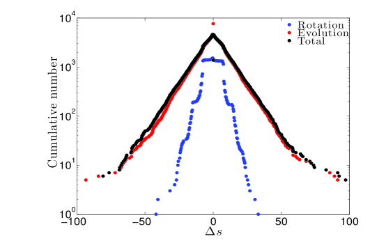
Figure fig:f2 shows the result of the analysis of the data. The figure presents the cumulative distribution of the total change in sunspot number $\Delta s$ using the complete data set (black), the change due to rotation of spots and groups onto and off the disc $\Delta s_{\rm r}$ (blue), and the changes due to the evolution of spots and groups $\Delta s_{\rm e}$ (red). The distributions of the total change $\Delta s$ and change due to evolution $\Delta s_{\rm e}$ are very similar, and both clearly show the Laplace distribution of Equation (eq:pop_law). The distribution of $\Delta s_{\rm r}$ exhibits significant falls in number at $\Delta s_{\rm r}=\pm 10k,\pm 20k,...$, which may be attributed to entire sunspot groups rotating onto and off the disc (groups are weighted with a factor of 10 in the definition of the international sunspot number – see Equation (eq:issn)).

An important feature of Figure fig:f2 is that the number of changes due to rotation onto and off the visible disc is at least an order of magnitude smaller than the number of changes due to evolution. There are too few changes associated with active regions rotating onto and off the visible disc for this to influence the overall distribution of changes in sunspot number. It is very unlikely that the observed double exponential distribution of changes, for days on which the sunspot number does change, is influenced by the small number of active regions which rotate onto or off the disc in a day.

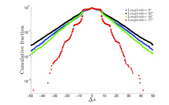
It is possible that the observed Laplace distribution arises from an averaging of locally non-exponential distributions across the disk. To test this we also calculate the cumulative fraction of changes occurring in particular 26^∘ strips on the disc. In other words, we identify the active regions in the strips on a given day, and calculate the sunspot number due to these regions only. On the next day we identify the regions in the strips, and again count the sunspot number due to these regions. The difference between these two counts is the change in sunspot number in a day occurring in the particular strips. This count includes both changes due to rotations into and out of the strips, and changes due to evolution in the strips. Figure fig:f2x shows the results. Changes occurring in the region $(-13^{\circ},0^{\circ})$ and $(0,13^{\circ})$ are in blue, changes occurring in the region $(-35^{\circ},-22^{\circ})$ and $(22,35^{\circ})$ are in black, changes occurring in the region $(-57^{\circ},-44^{\circ})$ and $(44,57^{\circ})$ are in green, and changes occurring at the limbs (i.e. $(-90^{\circ},-77^{\circ})$ and $(77,90^{\circ})$) are in red. Figure fig:f2x shows that changes associated with regions in a restricted range of longitudes reproduce the observed Laplace distribution. The exception is the distribution of changes at each limb, which shows large falls in probability due to changes in the number of groups in the strips, and a significantly smaller proportion of large changes in sunspot number. Presumably these differences arise due to the difficulty of accurately observing sunspot regions at the limb, and in particular, resolving the number of individual spots in a group. This may explain why this particular distribution is dominated by changes in the number of groups.

Figure fig:f2x shows that the observed Laplace distribution in total changes does not arise from averaging over non-exponential local distributions in particular strips. The conclusion is that the Laplace distribution form is representative of changes in daily sunspot number due to the local evolution of sunspot groups on the Sun. It reflects the physical processes occurring.

3 Daily Change in Sunspot Number

Section:Section2

3.1 A Conditional Distribution for Daily Change in Sunspot Number

Section:Section3.1 Pop (2012) investigated the daily change in sunspot number $\Delta s$ using data over complete cycles, which involve days with a range of different initial values $s$ of the sunspot number at each change. The phenomenological rule represented by Equation (eq:pop_law) was found to hold to a very good approximation for the range $10<\Delta s<60$ over the last 14 cycles, although departures from the rule for small changes in sunspot number were noted. This departure may be attributed to the discrete nature of sunspot number, which means that the minimum sunspot number larger than zero is $11k$ (where $k$ is typically less than unity). This causes a discrete jump in the tabulated daily values of the international sunspot number from zero to seven (and implies that the average value of $k$ used by observers is $k=0.64$). Departures for large changes in sunspot number were also noted. This may be attributed to the finite size of the sunspot number over any cycle. Large negative changes in sunspot number are unlikely because the sunspot number is unlikely to have a sufficiently large value at any given time over a cycle to allow that change.

The distribution of a change $\Delta s$ on a given day is dependent on the value of sunspot number on that day. To model this we introduce transition probabilities

$$\ilabel{eq:trans1}p(s\rightarrow s^{\prime}|s)=p(s^{\prime},s)$$ (7)

for changes from an initial sunspot number $s$ to a final sunspot number $s^{\prime}$ on a day, given that the sunspot number is initially $s$. The function on the right hand side is a conditional distribution, and in Section subsection:transition we consider a suitable functional form for this distribution. In Section subsection:relationship we relate the chosen form of the conditional distribution $p(s^{\prime},s)$ and Pop’s exponential distribution $f(\Delta s)$ of changes over complete cycles, and demonstrate how to estimate parameters from the data, for the proposed conditional distribution.

3.2 The Form of the Conditional Distribution

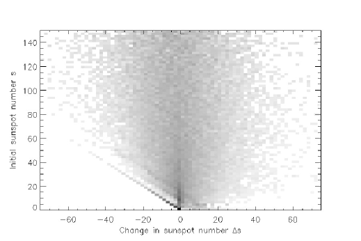
subsection:transition To gain insight into a suitable function form for the conditional distribution in Equation (eq:trans1) we re-examine the data. Figure fig:2x is a two-dimensional (2–D) histogram $N(\Delta s,s)$ of the number of days for which the sunspot number simultaneously has the value $s$ (enumerated along the vertical axis), and increases by $\Delta s$ to the next day (horizontal axis), for the NGDC data for 1815-2010. The bins are chosen to be of size two in $\Delta s$ and $s$, and the figure shows the normalised histogram

$$p_{i,j}=N(\Delta s_{i},s_{j})/\sum_{i}N(\Delta s_{i},s_{j}),$$ (8)

so that the greyscale density along each row shows the relative probability of a given change $\Delta s_{i}$, for the given initial sunspot number $s_{j}$. A nonlinear scaling is applied to the greyscale density, to better show the bins with small numbers of days. Figure fig:2x illustrates the influence of the lower boundary $\Delta s=-s$ required by the non–negativity of sunspot number. The distribution is relatively symmetric about $\Delta s=0$ for any given initial sunspot number $s$, except for an excess of days at the $\Delta s=-s$ boundary (which correspond to changes leading to a zero sunspot number), and an excess of days with no change (i.e. $\Delta s=0$).

Based on Figure fig:2x, a suitable approximate model form for Equation (eq:trans1) is a simple exponential distribution symmetric about $\Delta s=0$ for each value of $s$, with the same coefficient in the exponent for both negative and positive changes. The (asymmetric) non–negativity of sunspot number may be imposed by requiring that transitions producing a negative final sunspot number $(s^{\prime}<0)$ lead to zero sunspot number $(s^{\prime}=0)$ instead. This may be written as:

eq:pop˙law˙cond$$p(s^{\prime},s) = D\exp\left[-(s-s^{\prime})/E\right]\mathbb{I}(s^{\prime}<s)+D\exp\left[(s-s^{\prime})/E\right]\mathbb{I}(s^{\prime}>s)$$ (9)

$$+G\delta(s^{\prime})+H\delta(s^{\prime}-s),$$

where $D,\,E,\,F,\,G$, and $H$ are constants, and where the two terms involving delta functions describe the excess of days with changes leading to zero final sunspot number, and the excess of days on which the sunspot number does not change, respectively. The data show that for the observed changes in daily sunspot number for 1850–2011 the fraction of negative and positive jumps are approximately equal (42$\%$ and $41\%$ respectively), so we assume the same symmetry holds for each value of $s$ in Equation (eq:pop_law_cond):

$$\int_{0}^{s}p(s^{\prime},s)ds^{\prime}=\int_{s}^{\infty}p(s^{\prime},s)ds^{\prime}.$$ (10)

Normalising over all final sunspot numbers $s^{\prime}$, i.e. requiring

$$\int_{0}^{\infty}p(s^{\prime},s)ds^{\prime}=1$$ (11)

leads to

$$D=\frac{1-H}{2E}$$ (12)

and

$$G=\frac{1}{2}(1-H){\rm e}^{-s/E}.$$ (13)

The model conditional distribution (Equation (eq:pop_law_cond)) then has two parameters, $E$ and $H$. The parameter $E$ determines the size of changes on days when there is a change (a typical value, based on the data, is $E\approx 10$). The parameter $H$ is the probability of no change in daily sunspot number.

3.3 Relating the Conditional Distribution and the Pop (2012) Distribution, and Parameter Estimation

subsection:relationship The overall distribution of changes $f(\Delta s)$ may be calculated from the transitional distribution (Equation (eq:pop_law_cond)) by integrating over all starting values $s$, i.e. calculating

$$\ilabel{eq:formula}f(\Delta s)=L\int_{0}^{\infty}p(s+\Delta s,s)g(s)ds,$$ (14)

where $L$ is a constant imposing normalisation over changes in sunspot number:

$$\ilabel{eq:deltanorm}\int_{-\infty}^{\infty}f(\Delta s)d\Delta s=1,$$ (15)

and $g(s)$ is the probability of an initial sunspot number $s$ in the observations. A suitable choice to approximately describe the distribution of sunspot number $g(s)$ over a complete solar cycle is an exponential (Noble and Wheatland, 2011)

$$g(s)=\frac{1}{\lambda}{\rm e}^{-s/\lambda},$$ (16)

where the mean value of daily sunspot number (based on observations for 1850–2011) is $\lambda=55$. Calculating the integral in Equation (eq:formula) gives

eq:modelchanges$$Lf(\Delta s)= \frac{1-H}{2E}{\rm e}^{\Delta s/E}\left[1+\frac{E}{\lambda}e^{\Delta s/\lambda}\right]\mathbb{I}(\Delta s<0)+\frac{1-H}{2E}{\rm e}^{-\Delta s/E}\mathbb{I}(\Delta s>0)$$ (17)

$$+H\delta(\Delta s)$$

and the normalisation by Equation (eq:deltanorm) implies

$$L=1+\frac{E(1-H)}{2(\lambda+E)}.$$ (18)

For the case of negative changes ($\Delta s<0$), Equation (eq:modelchanges) contains a term $\lambda^{-1}E{\rm e}^{\Delta s/\lambda}$ which makes the distribution $f(\Delta s)$ asymmetric about $\Delta s=0$, and which is produced by changes leading to zero sunspot number. The characteristic size of this term is $E/\lambda\approx 0.18$, suggesting that the asymmetry in the distribution in $\Delta s$ produced by the lower boundary $\Delta s=-s$ is not a strong effect. In the absence of the extra term the normalisation constant is $L=1$, and based on the data we find $L\approx 1.05$. Neglecting the extra term and setting $L=1$, the distribution of changes implied by the conditional distribution (Equation (eq:pop_law_cond)) is

eq:approxmodelchanges$$f(\Delta s)= \frac{1-H}{2E}{\rm e}^{\Delta s/E}\mathbb{I}(\Delta s<0)+\frac{1-H}{2E}{\rm e}^{-\Delta s/E}\mathbb{I}(\Delta s>0)+H\delta(\Delta s)$$ (19)

which is the same functional form as Equation (eq:pop_law), the Pop (2012) distribution of changes.

The correspondence between the conditional distribution (Equation (eq:pop_law_cond)) and the overall distribution of changes (Equation (eq:approxmodelchanges)) allows the parameters $E$ and $H$ of the conditional distribution to be estimated from the daily changes $\Delta s$ over a cycle using maximum likelihood. Specifically, the exponential coefficient $B$ (see Equation (eq:pop_law_cond)) estimated for the overall distribution may be taken as the estimate for coefficient $E$ in the conditional distribution, and the fraction of days $C$ with no change in sunspot number (see Equation (eq:pop_law_cond)) in the overall distribution may be taken as the estimate of the corresponding parameter $H$ in the conditional distribution.

4 Simulating Sunspot Numbers

Section:Section3 In this section we apply the conditional distribution (Equation (eq:pop_law_cond)) in a Monte Carlo simulation of daily sunspot numbers $s_{i}=s(t_{i})$, where $t_{i}$ refers to a day. The daily random variation in sunspot number is described by the stochastic differential equation (stochastic DE)

$$\ilabel{eq:sde_{t}rans}\frac{ds}{dt}=\sum_{i=1}^{N}\Delta s_{i},$$ (20)

where $N$ is the number of days and the daily change $\Delta s_{i}$ is generated by sampling from the distribution

$$p(s^{\prime}_{i},s_{i})=p(s_{i}+\Delta s_{i},s_{i})$$ (21)

with $p(s^{\prime},s)$ given by Equation (eq:pop_law_cond).

To solve the stochastic DE (Equation (eq:sde_trans)) we need to sample from the conditional distribution $p(s^{\prime},s)$ given by Equation (eq:pop_law_cond), with our maximum likelihood estimate of the parameters $E$ and $H$. This is achieved as follows. For a given initial sunspot number $s$ and the estimates of $E$ and $H$ we generate a final sunspot number $s^{\prime}=s+\Delta s$ by generating an exponential random variable $\Delta s$ with parameter $E$ i.e. a random deviate $\Delta s$ distributed according to $\sim{\rm e}^{-\Delta s/E}$. A random variable $u$ which is uniformly distribution on $(0,1)$ is also generated, and then the final change $\Delta s$ is calculated according to the rule:

• if $u<0.5(1-H)$, then $\Delta s=-\Delta s$;

• if $u>0.5(1+H)$, then $\Delta s=\Delta s$;

• otherwise $\Delta s=0$.

This procedure assigns no change in sunspot number (i.e. $\Delta s=0$) with probability $H$, and the remaining changes are exponentially distributed over positive and negative $\Delta s$ with equal total probability. The mean absolute size of changes (on days when $\Delta s\neq 0$) is $E$. Finally, to prevent the final sunspot number $s^{\prime}=s+\Delta s$ from being negative, if $s+\Delta s<0$, then we take $\Delta s=-s$.

This procedure assigns values correctly according to Equation (eq:pop_law_cond). Equation (eq:sde_trans) is solved for a given initial sunspot number $s_{0}$ at time $t_{0}$ by generating a sequence of transitions $\Delta s_{i}$ (with $i=1,2,...,N$) according to this recipe, and adding these successively to $s_{0}$.

This model accounts for the stochastic variation in sunspot number according to the conditional distribution given by Equation (eq:pop_law_cond), but it does not account for the secular or long time-scale variation of the sunspot number over a solar cycle (the “shape” of the cycle). Recently Noble and Wheatland (2011) presented a method for modelling the solar cycle variation in a general Fokker-Planck description of stochastic variation in sunspot number, and the same procedure is applied here. A term may be added to the stochastic DE (Equation (eq:sde_trans)) causing the fluctuating sunspot number to return to a prescribed time evolution $\theta(t)$:

$$\ilabel{eq:sde_{s}ec_{t}rans}\frac{ds}{dt}=\kappa\left[\theta(t)-s\right]+\sum_{i=1}^{N}\Delta s_{i}.$$ (22)

The function $\theta(t)$ is referred to as the driver function, and factor $\kappa$ is the rate at which sunspot number $s$ returns to the value specified by the driver function. The two terms on the right hand side of Equation (eq:sde_sec_trans) are deterministic and stochastic terms, respectively. Equation (eq:sde_sec_trans) is solved for a given initial sunspot number $s_{0}$ by adding daily stochastic transitions $\Delta s_{i}$ in the same way as for Equation (eq:sde_trans). In between the transitions the sunspot number is evolved according to Equation (eq:sde_sec_trans) with just the deterministic term included. The solution to the differential equation with just the deterministic term is

$$\ilabel{eq:sde_{s}ec_{s}ol}s^{*}(t)={\rm e}^{-\kappa(t-t_{i})}\left\{s_{i}+\kappa\int_{t_{i}}^{t}\theta(t^{\prime}){\rm e}^{\kappa t^{\prime}}dt^{\prime}\right\},$$ (23)

where $s_{i}=s(t_{i})$ is the value of the sunspot number on the most recent day, and $t_{i}<t<t_{i+1}$.

To summarise, the procedure for simulating the sunspot number evolution for day $i+1$, given the sunspot number $s_{i}$ on day $i$, is to evaluate a deterministic value for the sunspot number $s^{*}(t_{i+1})$ using Equation (eq:sde_sec_sol), to generate a random change $\Delta s_{i+1}$ using Equation (eq:pop_law_cond) with initial sunspot number $s=s^{*}(t_{i+1})$, and then the sunspot number on day $i+1$ is $s_{i+1}=s^{*}(t_{i+1})+\Delta s_{i+1}$.

The driver function $\theta(t)$ in the deterministic term in Equation (eq:sde_sec_trans) represents the functional form of the solar cycle variation in sunspot number, i.e. the shape of a cycle. The driver function describes basic empirical features of a solar cycle, such as the time taken to reach maximum, the size of the maximum, and so on. Additionally, $\theta(t)$ may account for detailed features of the shape of a cycles such as the Gnevyshev Gap (Gnevyshev, 1967). Here we use a function introduced by Hathaway, Wilson, and Reichmann (1994, hereafter HWR94):

$$\ilabel{eq:hath}\theta(t)=\frac{a\left(t-t_{0}\right)^{3}}{\exp\left[-(t-t_{0})^{2}/b^{2}\right]-c},$$ (24)

where $t_{0}$ is the start time for a cycle, and $a$, $b$, and $c$ represent the cycle amplitude, period, and asymmetry, respectively. Equation (eq:hath) was used by Noble and Wheatland (2012) to investigate daily variation in sunspot number, and to forecast sunspot number and solar cycles. A statistical procedure for calculating estimates of the parameters $a$, $b$, $c$, and $\kappa$ from daily sunspot data, and the values of the estimates for cycles 11–23, was given in Noble and Wheatland (2012). Here we re–use these parameter estimates describing the shapes of the cycle to simulate three recent solar cycles (21, 22, and 23).

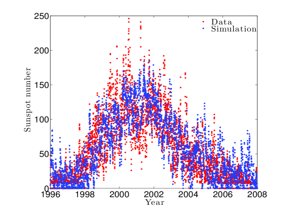
Figure fig:f4 shows the daily sunspot numbers over cycle 23, for the years 1996 to 2008 (red points), and our simulation of sunspot numbers for this cycle based on Equation (eq:sde_sec_trans) (blue points). The HWR94 driver function, Equation (eq:hath), enforces the secular variation in the solar cycle, with the parameter values $a=7.82\times 10^{-8}$, $b=1514$, $c=0.222$, and $\kappa=0.086$ (taken from Table I in Noble and Wheatland (2012)). We also use the estimates $E=8.78$ and $H=0.149$ for the conditional distribution (Equation (eq:pop_law_cond)), which are maximum likelihood values on the changes in daily sunspot data for cycle 23, as discussed in Section Section:Section2. For the HWR94 driver function it is not possible to solve Equation (eq:sde_sec_sol) analytically, and instead we integrate

$$\frac{ds}{dt}=\kappa\left[\theta(t)-s\right]$$ (25)

numerically using a fourth order Runge-Kutta scheme (Press et al., 1992).

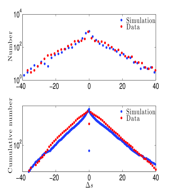
Figure fig:f5 shows the daily changes in sunspot number for cycle 23 (red points), and the corresponding changes in our simulation (blue points). The upper panel of Figure fig:f5 shows the distribution of changes and the lower panel shows the cumulative distribution in the same format as Figure fig:f1. Figure fig:f5 confirms that the simulation of daily sunspot number over cycle 23 based on the stochastic DE (Equation (eq:sde_sec_trans)) and the conditional distribution (Equation (eq:pop_law_cond)), together with the HWR94 model for the shape of the solar cycle, generates a distribution of changes $f(\Delta s)$ over the cycle that closely resembles the exponential form identified by Pop (2012).

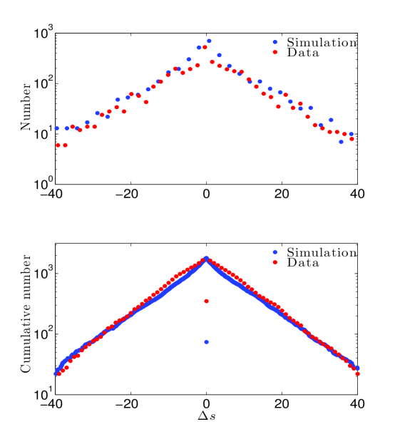
Figure fig:f6 presents the results of the simulation procedure for cycle 22 (years 1986 to 1996) in the same format as Figure fig:f5. The parameter estimates for the HWR94 driver function are $a=14.1\times 10^{-8}$, $b=1368$, $c=0.33$, and $\kappa=0.073$, again taken from Table I in Noble and Wheatland (2012). The estimates $E=10.4$ and $H=0.096$ are used for the parameters in the conditional distribution Equation (eq:pop_law_cond), based on maximum likelihood applied to the daily data for cycle 22.

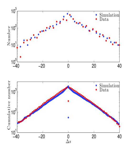
Figure fig:f7 presents the results of the simulation procedure for cycle 21 (years 1976 to 1986), again in the same format as Figure fig:f5. The parameter estimates for the HWR94 driver function are $a=12.2\times 10^{-8}$, $b=1414$, $c=0.490$, and $\kappa=0.073$, again taken from Table I in Noble and Wheatland (2012). The maximum likelihood estimates $E=10.6$ and $H=0.098$ are used for the parameters in the conditional distribution (Equation (eq:pop_law_cond)).

Figures fig:f6 and fig:f7 confirm that the simulation procedure succeeds in reproducing the phenomenological exponential rule for daily changes in sunspot number when applied to cycles 22 and 21, respectively.

5 Discussion

Section:Section5 This paper establishes that the observed Laplace, or double exponential distribution of changes $\Delta s$ in daily sunspot number $s$ (for days on which the sunspot number does change) recently identified by Pop (2012), is due to the evolution of observed sunspot groups (i.e. group formation, spot splitting, spot/group decay) rather than being due to the artificial variation caused by groups rotating onto and off the visible disc. The implication is that the distribution has a physical basis. Sunspot emergence, evolution, and eventual decay produces daily changes in sunspot number which may be positive or negative, and changes of this kind in separate active regions may add or cancel. The sum of these daily changes, remarkably, produces a simple Laplace distribution, with a marked excess of days with no change in sunspot number.

In this paper we show also how to simulate daily sunspot number via a Monte Carlo method, using a conditional distribution based on the exponential rule together with a model for the solar cycle variation in sunspot number. The conditional distribution $p(s^{\prime},s)$ introduced describes the probability of a change from a current sunspot number $s$ to a value $s^{\prime}=s+\Delta s$ in one day, given the initial sunspot number, and ensures that $s^{\prime}\geq 0$. The simulation procedure involves calculating a secular or deterministic change in sunspot number due to the underlying solar cycle, and then adding a random change in sunspot number according to the conditional distribution. The Monte Carlo method is demonstrated in application to three recent solar cycles (cycles 21, 22, and 23). The simulated sunspot numbers exhibit a distribution of changes $f(\Delta s)$ over each cycle that closely reproduces the Laplace distribution identified by Pop (2012).

It is interesting to consider possible explanations for the observed Laplace distribution. The origin of the surface changes in sunspot number described by the rule are changes in the structure of the subphotospheric magnetic fields, which are not directly amenable to observation (Thomas and Weiss, 1991), although local helioseismology is beginning to provide some insights (Gizon and Birch, 2005). In the absence of detailed physical models for the surface changes provided by this field evolution, it may be possible to construct statistical models for daily changes in sunspot number based on simple statistical descriptions of spot and group evolution, for given numbers of spots and groups. For example, probabilities could be assigned to given spots or groups increasing or decreasing their number in a day. Such a description may be modelled by a type of birth–death process, which have been used in the natural and social sciences (e.g. see for example Gillespie1992). It may also be possible to use other known statistical rules for the distribution and evolution of spot groups, for example the log–normal distribution of spot areas (Bogdan et al. 1988), and various rules for the decay rate of sunspot area (in area per unit time) per sunspot within a group (see 2003A&ARv..11..153S). Given the complexity of the combinations implied by this consideration of possible modelling, we note again how remarkable it is that a simple double exponential form arises. We leave the development of a detailed model to a future investigation.

Acknowledgements

P. N. gratefully acknowledges a University of Sydney Postgraduate Scholarship.

Figure 1.: Histograms showing the observed numbers of daily changes in sunspot number for 1850–2011 (red points), and the model distribution for the changes defined by Equation (eq:pop_law). The upper panel shows the number of days with a given change, for positive and negative changes, and the lower panel shows the corresponding cumulative number. fig:f1

Figure 2.: The cumulative distribution of the changes in daily sunspot number due to rotation of sunspot regions onto and off the disc (blue), the change due to evolution of regions (red), and the total change (black). fig:f2

Figure 3.: The cumulative distribution of daily change sunspot number calculated in four 26^∘ degree strips. The daily changes in sunspot number in the strip from $-13^{\circ}$ to $13^{\circ}$ are shown in blue, the changes in the strip from $-35^{\circ}$ to $-22^{\circ}$ and from $22^{\circ}$ to $35^{\circ}$ are shown in black, the change in the strip from $-57^{\circ}$ to $-44^{\circ}$ and from $44^{\circ}$ to $57^{\circ}$ are in green, and changes in the strip from $-90^{\circ}$ to $-77^{\circ}$ and from $77^{\circ}$ to $90^{\circ}$ are shown in red. fig:f2x

Figure 4.: Two dimensional histogram showing the fraction of days on which the sunspot number changes by $\Delta s$ (horizontal axis), given the initial value $s$ (vertical axis). The histogram has been normalised to represent an equal number of days at each initial sunspot number $s$. fig:2x

Figure 5.: The observed daily sunspot numbers over cycle 23 (red points), and a simulation of the sunspot numbers using the procedure outlined in Section Section:Section3. The parameters for the modelling of the shape of the cycle are taken from Noble and Wheatland (2012). fig:f4

Figure 6.: Histograms of the observed daily changes in the sunspot number for cycle 23 (see Figure fig:f4), and for our simulation of the sunspot numbers. The red points show the data and the blue points the simulation. The upper panel shows the numbers of days with the given change in sunspot number and the lower panel shows the corresponding cumulative distribution. fig:f5

Figure 7.: Changes in daily sunspot number for solar cycle 22 (red points) and for our simulation of the cycle (blue points). The upper panel shows the numbers of days with the given change, and the lower panel is the corresponding cumulative distribution. fig:f6

Figure 8.: Changes in daily sunspot numbers for solar cycle 21 (red points) and for our simulation of the cycle (blue points). The upper panel shows the number of days with the given change, and the lower panel is the corresponding cumulative distribution. fig:f7

References

- Bogdan et al. (1988) Bogdan, T.J., Gilman, P.A., Lerche, I., Howard, R.: 1988, Astrophys. J. 327, 451.
- Bruzek and Durrant (1977) Bruzek, A., Durrant, C.J.: 1977, Illustrated Glossary for Solar and Solar-Terrestrial Physics, D. Reidel Publishing Company, Dordrecht, 70.
- Committee on the Societal and Economic Impacts of Severe Space Weather Events (2008) Committee on the Societal and Economic Impacts of Severe Space Weather Events: 2008, Severe Space Weather Events: Understanding Societal and Economic Impacts, The National Academies Press, Washington, DC.
- Eliason (1993) Eliason, S. R.: 1993, Maximum Likelihood Estimation; Logic and Practice, Sage Publications, London, 8.
- Gillespie (1992) Gillespie, D. T.: 1992, Markov Processes, Academic Press, San Diego, 375.
- Gizon and Birch (2005) Gizon, L., Birch, A.C.: 2005, Living Rev. Solar Phys. 2 (6), http://solarphysics.livingreviews.org/Articles/lrsp-2005-6/.
- Gnevyshev (1967) Gnevyshev, M.N.: 1967, Solar Phys. 1, 107.
- Hathaway, Wilson, and Reichmann (1994) Hathaway, D. H., Wilson, R. M., Reichmann, E. J.: 1994, Sol. Phys.151, 177.
- Kaiser et al. (2008) Kaiser, M.L., Kucera, T.A., Davila, J.M., St. Cyr, O.C., Guhathakurta, M., Christian, E.: 2008, Space Sci. Rev. 136, 5.
- Lepreti, Kossobokov, and Carbone (2009) Lepreti, F., Kossobokov, V.G., Carbone, V.: 2009, Int. J. Mod. Phys. B 23, 5609.
- Noble and Wheatland (2011) Noble, P.L., Wheatland, M.S.: 2011, Astrophys. J. 732, 5.
- Noble and Wheatland (2012) Noble, P.L., Wheatland, M.S.: 2012, Solar Phys. 276, 363.
- Odenwald, Green, and Taylor (2006) Odenwald, S., Green, J., Taylor, W.: 2006, Adv. Space Res. 38, 280.
- Ossendrijver (2003) Ossendrijver, M.: 2003, A&A Rev. 11, 287.
- Petrovay (2010) Petrovay, K.: 2010, Living Rev. Solar Phys. 7 (6), http://solarphysics.livingreviews.org/Articles/lrsp-2010-6/.
- Pop (2012) Pop, M.-I.: 2012, Solar Phys. 276, 351.
- Press et al. (1992) Press, W.H., Teukolsky, S.A., Vetterling, W.T., Flannery, B.P.: 1992, Numerical Recipes in C: The Art of Scientific Computing, 2nd ed., Cambridge University Press, Cambridge, 710.
- Solanki (2003) Solanki, S.K.: 2003, A&A Rev. 11, 153.
- Thomas and Weiss (1991) Thomas, J. H., Weiss, N. O.: 1991, In: Thomas, J. H., Weiss, N. O. (eds.), Sunspots: Theory and Observations, Kluwer Academic Publishers, Dordrecht, The Netherlands, 3.
- Tobias (2002) Tobias, S.M.: 2002, Phil. Trans. Roy. Soc. London A 360, 2741.
- Snodgrass and Ulrich (1990) Snodgrass, H.B., Ulrich, R.K.: 1990, Astrophys. J. 351, 309.