Average position in quantum walks with a U(2) coin

Abstract

We investigated discrete-time quantum walks with an arbitary unitary coin. Here we discover that the average position $\left\langle x\right\rangle=\max(\left\langle x\right\rangle)\sin(\alpha+\gamma)$, while the initial state is $1/\sqrt{2}(\mid 0L\rangle+i\mid 0R\rangle)$. We prove the result and get some symmetry properties of quantum walks with a U(2) coin with $\mid 0L\rangle$ and $\mid 0R\rangle$ as the initial state.

I introduction

Quantum walks (QWs) were first introduced in 1993 Aharonov as generalization of classical random walks. According to the time evolution, QWs can be devided into discrete-time and continuous-time Farhi-continue-time QWs. Recently, both continuous-time Childs-continue-universal and discrete-time Lovett-discrete-universal QWs are found to be universal for quantum computation. A number of quantum algorithms based on QWs have already been proposed in Shenvi2003 ; Childs2004 ; Ambainis ; Ambainis2004 ; Childs2003 ; Childs2002 . In addition, QWs in graph Aharonov-1 , on a line with a moving boundary Kwek , with multiple coins Brun-1 or decoherent coins Brun have been discussed also.

QWs using a SU(2) coin was introduced by Chandrashekar, et al. Chandrashekar , where the standard deviation and measurement entropy properties were discussed. Here we discuss the symmetry and average position properties for the QWs with a U(2) coin.

II hadamard quantum walks

In this paper, we always discuss within the discrete-time QWs . The total Hilbert space for QWs is given by $\mathcal{H}\equiv\mathcal{H}_{P}\otimes\mathcal{H}_{C}$, where $\mathcal{H}_{P}$ is spanned by the orthonormal states $\left\{\mid x\rangle\right\}$ and $\mathcal{H}_{C}$ is the two-dimensional coin space spaned by two orthonormal states $\mid L\rangle$ and $\mid R\rangle.$

Each step of the QWs can be splitted into two operations: the evolution of coin state and the particle movement according to the coin state.

Here the Hadamard walk, the coin is evolved by applying the Hadamard operation:

$$H=\frac{1}{\sqrt{2}}\begin{pmatrix}1&1\\ 1&-1\end{pmatrix},$$

the particle movement operator is given by

$$S=e^{ip\sigma_{z}}=\sum_{x}S_{x},$$ (1)

where $p$ is the momentum operator, $\sigma_{z}$ is the Pauli-$z$ operator,

$$\hat{S}_{x}=\mid x+1\rangle\langle x\mid\otimes\mid R\rangle\langle R\mid+\mid x-1\rangle\langle x\mid\otimes\mid L\rangle\langle L\mid.$$ (2)

Therefore, after $t$ steps QWs

$$\mid\Psi_{t}\rangle =\left[S(I_{P}\otimes H)\right]^{t}\mid\Psi_{0}\rangle$$ (3)

$$=\left[\sum_{x}S_{x}(I_{P}\otimes H_{C})\right]^{t}\mid\Psi_{0}\rangle,$$

where $\mid\Psi_{in}\rangle$ is the initial state of the system.

III generalized discrete time quantumw walks

An arbitrary one-qubit unitary operation can be written as a U(2) matrix:

$$U_{\alpha,\beta,\gamma,\theta}=e^{i\theta}\left(\begin{array}[]{cc}e^{i\alpha}\cos\beta,&-e^{-i\gamma}\sin\beta\\ e^{i\gamma}\sin\beta,&e^{-i\alpha}\cos\beta\end{array}\right)$$ (4)

For example, the Hadamard operator can be described in the form $H=U_{\frac{\pi}{2},\frac{\pi}{4},\frac{\pi}{2},-\frac{\pi}{2}}$. By replacing the Hadamard coin with an operator $U_{\alpha,\beta,\gamma,\theta}$, we can obtain the generalized QWs Chandrashekar , which can be written as

$$\mid\Psi_{t}\rangle=\left[S(I_{P}\otimes U_{\alpha,\beta,\gamma,\theta})\right]^{t}\mid\Psi_{0}\rangle$$ (5)

Lemma 1.

The quantum walks have the same probability distribution with a U(2) coin or a SU(2) coin which has the same parameters $\alpha$, $\beta$ and $\gamma$ in the U(2) martrix.

Proof.

The SU(2) coin operator can be written as

$$U_{\alpha,\beta,\gamma}^{S}=\left(\begin{array}[]{cc}e^{i\alpha}\cos\beta,&-e^{-i\gamma}\sin\beta\\ e^{i\gamma}\sin\beta,&e^{-i\alpha}\cos\beta\end{array}\right),$$ (6)

Then the U(2) coin $U_{\alpha,\beta,\gamma,\theta}=e^{i\theta}U_{\alpha,\beta,\gamma}^{S}$. The probability distribution for QWs with a U(2) coin after $t$ steps:

$$P(x,t) =|\langle x|\Psi_{t}\rangle|^{2}=|e^{it\theta}\langle x\mid\Psi_{t}^{S}\rangle|^{2}$$ (7)

$$\equiv P^{S}(x,t),$$

where $\mid\Psi_{t}^{S}\rangle$ and $P^{S}(x,t)$ are the state and the probability distribution for QWs with a SU(2) coin after $t$ steps respectively.∎

Corollary 2.

The average position is the same in quantum walks with a U(2) coin and a SU(2) coin if the two coins have the same parameters $\alpha$, $\beta$ and $\gamma$ with the U(2) coin.

Proof.

From Lemma 1, we can know that the average position for a U(2) coin $\langle x\rangle=\sum_{x}xP(x,t)=\sum_{x}xP^{S}(x,t)\equiv\langle x\rangle^{S}$, where $\langle x\rangle^{S}$ is the average position for QWs with a SU(2) coin. ∎

With corollary 2, if we want to know the average position property in QWs with an arbitray unitary operator, we only need to study the quantum walk with a SU(2) coin instead, for the rest part of this paper, we always use the SU(2) coin as denoted in Eq. (6).

Following the analysis in Ref. Nayak , the state after $t$ steps QWs with a SU(2) coin

$$\mid\Psi_{t}\rangle=\left[S(I_{P}\otimes U_{\alpha,\beta,\gamma}^{S})\right]^{t}\mid\Psi_{0}\rangle,$$ (8)

the spatial Fourier transformation for of the wave function $\Psi(x,t)$ over $\mathscr{\mathcal{Z}}$ is given by

$$\begin{aligned} \tilde{\Psi}(k,t)&=\sum_{x=-\infty}^{\infty}\Psi(x,t)e^{ikx}\end{aligned},$$ (9)

where $k\in[-\pi,\pi]$. We can know

$$\tilde{\Psi}(k,t)=(M_{k})^{t}\tilde{\Psi}(k,0),$$ (10)

where

$$M_{k} =e^{ik}M_{+}+e^{-ik}M_{-}$$ (11)

$$=\left(\begin{array}[]{cc}e^{-i(k-\alpha)}\cos\beta,&-e^{-i(k+\gamma)}\sin\beta\\ e^{i(k+\gamma)}\sin\beta,&e^{i(k-\alpha)}\cos\beta\end{array}\right).$$

The eigenvalues of $M_{k}$ is

$$\begin{cases}\lambda_{a}=e^{-iw}\\ \lambda_{b}=e^{iw}\end{cases},$$ (12)

where $\cos w=\cos(k-\alpha)\cos\beta$. And the eigenstates

$$\begin{cases}\tilde{\Psi}_{k}^{a}&=\frac{1}{C_{k}^{a}}\left(\begin{array}[]{c}P_{k}\\ Q_{k}^{a}\end{array}\right)\\ \tilde{\Psi}_{k}^{b}&=\frac{1}{C_{k}^{b}}\left(\begin{array}[]{c}P_{k}\\ Q_{k}^{b}\end{array}\right)\end{cases},$$ (13)

where

$$\begin{aligned} \begin{cases}P_{k}=-e^{-i(k+\gamma)}\sin\beta\\ Q_{k}^{a}=-i\sin\omega_{k}+i\sin(k-\alpha)\cos\beta\\ Q_{k}^{b}=i\sin\omega_{k}+i\sin(k-\alpha)\cos\beta\end{cases}\end{aligned},$$ (14)

$$C_{k}^{a} =\sqrt{P_{k}^{*}P_{k}+(Q_{k}^{a})^{*}Q_{k}^{a}}$$ (15)

$$=\sqrt{2(\sin^{2}\omega_{k}-\cos\beta\sin(k-\alpha)\sin\omega_{k})},$$

$$C_{k}^{b} =\sqrt{P_{k}^{*}P_{k}+(Q_{k}^{b})^{*}Q_{k}^{b}}$$ (16)

$$=\sqrt{2(\sin^{2}\omega_{k}+\cos\beta\sin(k-\alpha)\sin\omega_{k})}.$$

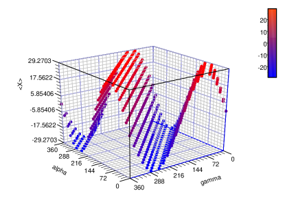
Figure 1: The average of position $\left\langle x\right\rangle$ for quantun walks after $t=100$ steps with a SU(2) coin, where$\beta=\pi/6$.

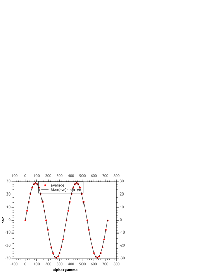
Figure 2: (red dot)The average of position with $\alpha+\gamma$ after $100$ steps quantum walk when $\beta=\pi/6$, (line) $f(\phi)=\max(\left\langle x\right\rangle)\sin(\phi)$.

IV the average position in quantum walks

Fig. 1 and Fig. 2 show the average position after $t=100$ steps QWs with a SU(2) coin in the case of $\beta=\pi/6$, while the initial state is $1/\sqrt{2}(\mid 0L\rangle+i\mid 0R\rangle)$. From Fig. 1, we can know that $\left\langle x\right\rangle$ only depends on the sum of $\alpha$ and $\gamma$. Fig. 2 shows that the actual $\left\langle x\right\rangle$ exactly match the function of $f(\phi)=\max(\left\langle x\right\rangle)\sin(\phi)$, then we conject that $\left\langle x\right\rangle=G(\beta,t)\sin(\alpha+\gamma)$.

V proof in methematics

Theorem 3.

The probability distribution for quantum walks with a SU(2) coin is independent on the parameter $\alpha$ and $\gamma$, when the initial state is $\mid 0L\rangle$ or $\mid 0R\rangle.$ i.e.

$$\begin{aligned} \begin{cases}P_{\mid 0L\rangle}(\alpha,\beta,\gamma,x,t)=P_{\mid 0L\rangle}(\beta,x,t)\\ P_{\mid 0R\rangle}(\alpha,\beta,\gamma,x,t)=P_{\mid 0R\rangle}(\beta,x,t)\end{cases}\end{aligned},$$ (17)

for any $\alpha$ and $\gamma.$

Proof.

If the initial state $\mid\Psi_{0}\rangle=\mid 0L\rangle$, then $\tilde{\Psi}(k,0)=\left(\begin{array}[]{c}1\\ 0\end{array}\right)$. The probability of $\mid x\rangle:$

$$P_{\mid 0L\rangle}(\alpha,\beta,\gamma,x,t)$$ (18)

$$=P_{L}(\alpha,\beta,\gamma,x,t)+P_{R}(\alpha,\beta,\gamma,x,t)$$

$$=\frac{1}{4\pi^{2}}\int_{-\pi}^{\pi}\int_{-\pi}^{\pi}g_{L}(k_{1},k_{2},\alpha,\beta,\gamma,x,t)dk_{1}dk_{2}+$$

$$\qquad\frac{1}{4\pi^{2}}\int_{-\pi}^{\pi}\int_{-\pi}^{\pi}g_{R}(k_{1},k_{2},\alpha,\beta,\gamma,x,t)dk_{1}dk_{2},$$

where $g_{j}(k_{1},k_{2},\alpha,\beta,\gamma,x,t)=\tilde{\Psi}_{j}^{*}(k_{1},t)\tilde{\Psi}_{j}(k_{2},t)e^{i(k_{1}-k_{2})x}$, $j\in\{L,R\}$. If we set $h=k-\alpha$, then we can know $g_{j}(k_{1},k_{2},\alpha,\beta,\gamma,x,t)=g_{j}(h_{1},h_{2},\beta,x,t)$, and $g_{j}(h_{1},h_{2},\beta,x,t)=g_{j}(h_{1}\pm 2\pi,h_{2},\beta,x,t)=g_{j}(h_{1},h_{2}\pm 2\pi,\beta,x,t)$, then

$$P_{j}(\alpha,\beta,\gamma,x,t) =\frac{1}{4\pi^{2}}\int_{-\pi-\alpha}^{\pi-\alpha}\int_{-\pi-\alpha}^{\pi-\alpha}g_{j}(h_{1},h_{2},\beta,x,t)dh_{1}dh_{2}$$ (19)

$$=\frac{1}{4\pi^{2}}\int_{-\pi}^{\pi}\int_{-\pi}^{\pi}g_{j}(h_{1},h_{2},\beta,x,t)dh_{1}dh_{2}$$

$$=P_{j}(\beta,x,t).$$

Further more we can know $P_{\mid 0L\rangle}(\alpha,\beta,\gamma,x,t)=P_{\mid 0L\rangle}(\beta,x,t)$. In the same way, we can also get $P_{\mid 0R\rangle}(\alpha,\beta,\gamma,x,t)=P_{\mid 0R\rangle}(\beta,x,t)$. ∎

Theorem 4.

After t steps, we have

$$\begin{cases}\Psi_{\mid 0L\rangle}^{R}(x,t)+\Psi_{\mid 0R\rangle}^{L}(-x,t)\in i\mathbb{R}\\ \Psi_{\mid 0L\rangle}^{R}(x,t)-\Psi_{\mid 0R\rangle}^{L}(-x,t)\in\mathbb{R}\end{cases},$$ (20)

$$\begin{cases}\Psi_{\mid 0L\rangle}^{L}(x,t)+\Psi_{\mid 0R\rangle}^{R}(-x,t)\in\mathbb{R}\\ \Psi_{\mid 0L\rangle}^{L}(x,t)-\Psi_{\mid 0R\rangle}^{R}(-x,t)\in i\mathbb{R}\end{cases},$$ (21)

where $\Psi_{\mid n\rangle}^{m}(x,t)$ denotes the coefficient of the $\mid x\rangle\mid m\rangle$ state after $t$ steps quantum walk with the initail state $\mid n\rangle$.

Proof.

$$\Psi_{\mid 0L\rangle}^{R}(x,t)\pm\Psi_{\mid 0R\rangle}^{L}(-x,t)$$ (22)

$$=\frac{1}{2\pi}\int_{-\pi}^{\pi}\tilde{\Psi}_{\mid 0L\rangle}^{R}(k,t)e^{-ikx}dk\pm\frac{1}{2\pi}\int_{-\pi}^{\pi}\tilde{\Psi}_{\mid 0R\rangle}^{L}(k,t)e^{ikx}dk$$

$$=\frac{1}{2\pi}\int_{-\pi}^{\pi}\frac{Q_{k}^{a}}{(C_{k}^{a})^{2}}[P_{k}^{*}e^{-ikx}\mp P_{k}e^{ikx}][e^{-i\omega_{k}t}-e^{i\omega_{k}t}]dk.$$

As $Q_{k}^{a}\in i\mathbb{R}$, we can know $\Psi_{\mid 0L\rangle}^{R}(x,t)+\Psi_{\mid 0R\rangle}^{L}(-x,t)\in i\mathbb{R}$, and $\Psi_{\mid 0L\rangle}^{R}(x,t)-\Psi_{\mid 0R\rangle}^{L}(-x,t)\in\mathbb{R}.$ Similarly, we can get Eq. (21).∎

Corollary 5.

The symmetry property of distribution between quantum walks with a U(2) coin in initial state $\mid 0L\rangle$ and $\mid 0R\rangle$: For an arbitrary $t$, $P_{\mid 0L\rangle}^{R}(\beta,x,t)=P_{\mid 0R\rangle}^{L}(\beta,-x,t)$, $P_{\mid 0L\rangle}^{L}(\beta,x,t)=P_{\mid 0R\rangle}^{R}(\beta,-x,t)$.

Proof.

We set $\Psi_{\mid 0L\rangle}^{R}(x)=C+Di$, where $C,D\in\mathbb{R}$. From Theorem 4, we can know $\Psi_{\mid 0R\rangle}^{L}(-x)=-C+Di$, then we can know $P_{\mid 0L\rangle}^{R}(\beta,x,t)=P_{\mid 0R\rangle}^{L}(\beta,-x,t)$. Similarly, we can also get $P_{\mid 0L\rangle}^{L}(\beta,x,t)=P_{\mid 0R\rangle}^{R}(\beta,-x,t)$.∎

Theorem 6.

If the initial state $\mid\Psi_{0}\rangle=m\mid 0L\rangle+n\mid 0R\rangle$, where $|m|^{2}+|n|^{2}=1$, the probability at state $\mid xL\rangle$ or $\mid xR\rangle$ after $t$ steps quantum walk is

$$\begin{cases}P^{L}(x)=|m|^{2}P_{\mid 0L\rangle}^{L}+|n|^{2}P_{\mid 0R\rangle}^{L}-(e^{-i(\alpha+\gamma)}m^{*}n+e^{i(\alpha+\gamma)}mn^{*})G^{L}(\beta,x,t)\\ P^{R}(x)=|m|^{2}P_{\mid 0L\rangle}^{R}+|n|^{2}P_{\mid 0R\rangle}^{R}-(e^{-i(\alpha+\gamma)}m^{*}n+e^{i(\alpha+\gamma)}mn^{*})G^{R}(\beta,x,t)\end{cases},$$ (23)

where $G^{L}$ and $G^{R}$ are indepent of $\alpha$ and $\gamma$.

Proof.

The probability at state $\mid xL\rangle$ after $t$ steps:

$$P_{m\mid 0L\rangle+n\mid 0R\rangle}^{L}(x) =\frac{1}{4\pi^{2}}\int\int\tilde{\Psi}_{L}^{*}(k_{1},t)\tilde{\Psi}_{L}(k_{2},t)e^{i(k_{1}-k_{2})x}dk_{1}dk_{2}$$ (24)

$$=|m|^{2}P_{0L}^{L}(\beta,x,t)+|n|^{2}P_{0R}^{L}(\beta,x,t)-$$

$$\qquad(e^{-i(\alpha+\gamma)}m^{*}n\sum_{i=1}^{4}G_{i}+e^{i(\alpha+\gamma)}mn^{*}\sum_{i=1}^{4}G_{i}^{*}),$$

where

$$G_{1}(\beta,x,t) =\frac{1}{4\pi^{2}}\int\int e^{i(\omega_{h_{1}}-\omega_{h_{2}})t}\frac{1}{(C_{h_{1}}^{b}C_{h_{2}}^{b})^{2}}e^{i(h_{1}-h_{2})}\sin^{3}\beta e^{i(h_{1}-h_{2})x}e^{-ih_{1}}(Q_{h_{2}}^{b})^{*}dh_{1}dh_{2}$$ (25)

$$=\frac{1}{4\pi^{2}}\int\int\frac{(Q_{h_{2}}^{b})^{*}\sin^{3}\beta}{(C_{h_{1}}^{b}C_{h_{2}}^{b})^{2}}i\sin[(\omega_{h_{1}}-\omega_{h_{2}})+(h_{1}-h_{2})+(h_{1}-h_{2})x-h_{1}]dh_{1}dh_{2}\in R.$$

As the same of $G_{1}(\beta,x,t)$, we can know $G_{i}(\beta,x,t)\in R$, where $i\in\{1,2,3,4\}$. So Eq. (24) can be written as

$$P^{L}(x)=|m|^{2}P_{\mid 0L\rangle}^{L}+|n|^{2}P_{\mid 0R\rangle}^{L}-(e^{-i(\alpha+\gamma)}m^{*}n+e^{i(\alpha+\gamma)}mn^{*})G^{L}(\beta,x,t),$$ (26)

where $G^{L}(\beta,x,t)=\sum_{i=1}^{4}G_{i}$. In the same way as $P^{L}(x)$, we can get $P^{R}(x)$ in Eq. (23). ∎

Theorem 7.

If the initail state $\mid\Psi_{0}\rangle=1/\sqrt{2}(\mid 0L\rangle+i\mid 0R\rangle)$, The average position after $t$ steps quantum walk: $\left\langle x\right\rangle=G(\beta,t)\sin(\alpha+\gamma)$, where $G(\beta,t)$ only depends on $\beta$ and $t$.

Proof.

From Corollary 5, we can know

$$\begin{cases}\sum_{x=-t}^{t}x[P_{\mid 0L\rangle}^{R}(\beta,x,t)+P_{\mid 0R\rangle}^{L}(\beta,x,t)]=0\\ \sum_{x=-t}^{t}x[P_{\mid 0L\rangle}^{L}(\beta,x,t)+P_{\mid 0R\rangle}^{R}(\beta,x,t)]=0\end{cases}\text{.}$$ (27)

Using Eq. (27) and Theorem 6 we can know

$$\left\langle x\right\rangle =\sum_{x=-t}^{t}x(P^{L}(\alpha,\beta,\gamma,x,t)+P^{R}(\alpha,\beta,\gamma,x,t))$$ (28)

$$=G(\beta,t)\sin(\alpha+\gamma),$$

where $G(\beta,t)=-\sum_{x=-t}^{t}x[G^{L}(\beta,x,t)+G^{R}(\beta,x,t)]$ only depends on $\beta$ and $t$, regardless of $\alpha$ or $\gamma$. ∎

VI conclusions

In this paper, we discussed the properties of the average position in QWs with an arbitrary unitary coin. With a SU(2) coin, if the initial state is $\mid 0L\rangle$ or $\mid 0R\rangle$, the probability distribution is independent on $\alpha$ and $\gamma$. Some symmetry properties between different initial states $\mid 0L\rangle$ and $\mid 0R\rangle$ was prooved, we get that $P_{\mid 0L\rangle}^{R}(\beta,x,t)=P_{\mid 0R\rangle}^{L}(\beta,-x,t)$ and $P_{\mid 0L\rangle}^{L}(\beta,x,t)=P_{\mid 0R\rangle}^{R}(\beta,-x,t)$. If the initial state $\mid\Psi_{0}\rangle=1/\sqrt{2}(\mid 0L\rangle+i\mid 0R\rangle)$, we can know the average $\left\langle x\right\rangle=G(\beta,t)\sin(\alpha+\gamma)$, so if we replace the Hadamard operator with an arbitrary unitary operator, the average position is always not equal to $0$, unless $\alpha+\beta=n\pi,n\in\mathbb{Z}$.

References

• (1) Y. Aharonov, L. Davidovich, and N. Zagury, Phys. Rev. A 48, 1687 (1993).
• (2) E. Farhi, and S. Gutmann, Phys. Rev. A 58, 915 (1998)
• (3) A. M. Childs, Phys. Rev. Lett. 102, 180501 (2009).
• (4) N. B. Lovett, S. Cooper, M. Everitt, M. Trevers, and V. Kendon, Phys. Rev. A 81, 042330 (2010)
• (5) A. M. Childs, R. Cleve, E. Deotto, E. Farhi, S. Gutmann, and D. A. Spielman, Proceedings of the 35th ACM symposium on Theory of computing (ACM Press, New York), (2003), pp. 59-68.
• (6) N. Shenvi, J. Kempe, and K. Birgitta Whaley, Phys. Rev. A 67, 052307 (2003).
• (7) A. M. Childs, E. Farhi, and S. Gutmann, Quantum Information Processing, Vol. 1, pp. 35-43 (2002).
• (8) A. M. Childs and J. Goldstone, Phys. Rev. A 70, 022314 (2004).
• (9) A. Ambainis, arXiv:quant-ph/0403120.
• (10) A. Ambainis and J. Kempe, In Proceedings of the 16th ACM-SIAM symposium on Discrete algorithms, pp. 1099–1108, (2005).
• (11) D. Aharonov, A. Ambainis, J. Kempe, U. Vazirani, Proceeding STOC ’01 Proceedings of the thirty-third annual ACM symposium on Theory of computing, pp. 50 - 59 (2001).
• (12) L. C. Kwek and Setiawan, Phy. Rev A 84, 032319 (2011).
• (13) T. A. Brun, H. A. Carteret, and A. Ambainis, Phys. Rev. A 67, 052317 (2003).
• (14) T. A. Brun, H. A. Carteret, and A. Ambainis, Phys. Rev. A 67, 032304 (2003).
• (15) C. M. Chandrashekar, R. Srikanth, and R. Laflamme, Phy. Rev. A 77, 032306 (2008).
• (16) A. Nayak and A. Vishwanath, Technical Report, Center for Discrete Mathematics & Theoretical Computer Science (2000).