Scalar Resonances in the Non-linearly Realized
Electroweak Theory

Abstract

We introduce a physical scalar sector in a SU(2)$\otimes$U(1) electroweak theory in which the gauge group is realized non linearly. By invoking theoretical as well as experimental constraints, we build a phenomenologically viable model in which a minimum of four scalar resonances appear, and the mass of the CP even scalar is controlled by a vacuum expectation value; however, the masses of all other particles (both matter as well as vector boson fields) are unrelated to spontaneous symmetry breaking and generated by the Stückelberg mechanism. We evaluate in this model the CP-even scalar decay rate to two photons and use this amplitude to perform a preliminary comparison with the recent LHC measurements. As a result, we find that the model exhibits a preference for a negative Yukawa coupling between the top quark and the CP-even resonance.

I Introduction

The experimental programme for probing the Spontaneous Symmetry Breaking (SSB) mechanism of the Standard Model (SM) of particle physics has recently witnessed a major breakthrough with the simultaneous announcements by the ATLAS :2012gk and CMS :2012gu collaborations of the observation of a new bosonic particle with a mass of about $125$ GeV.

Though one cannot claim yet any significative discrepancy between the properties of this new particle and the expectations for the SM Higgs field, there is a $2\sigma$ evidence for an enhanced $\gamma\gamma$ channel (and slightly suppressed $WW$ and $ZZ$ channels), which, in a SM-like scenario, can be accounted for by a modified (possibly negative) Yukawa coupling and a moderate rescaling of the Higgs to vectors coupling Giardino:2012dp ; Ellis:2012hz ; Espinosa:2012im . To be sure, the LHC measurements of these processes will significantly improve in the near future, thus leading either to a full confirmation of the SM scenario or to the discovery of new physics beyond it. However, given the present situation, it is particularly important to compare the experimental data against all possible theoretically sound scenarios that can account for possible deviations of the particle couplings from the SM results.

A relatively unexplored model in this context is an electroweak theory in which the SU(2)$\otimes$U(1) gauge group is realized non-linearly. In fact, the usual Higgs mechanism Englert:1964et ; Higgs:1964ia ; Higgs:1964pj ; Guralnik:1964eu is based on a linear representation of the gauge group: Masses are generated by SSB through the appearance of a non-zero vacuum expectation value (vev) of a physical scalar field, triggered by the usual quartic (mexican hat) potential. On the other hand, in a model in which the gauge group is realized non-linearly, masses are generated via the Stückelberg mechanism Stueck , that is through the coupling with the flat connection of the gauge group. As a consequence, the couplings of a scalar resonance would not be related to the masses of the particles which it couples to, unlike those of the Higgs field(s) in the SM and extensions thereof.

In this paper we discuss in detail how one can include scalar resonances in the nonlinearly realized electroweak theory within the formalism based on the Local Functional Equation (LFE) Bettinelli:2008ey ; Bettinelli:2008qn ; Bettinelli:2007tq ; Bettinelli:2009wu ; Ferrari:2005va ; Ferrari:2004pd ; Bettinelli:2007kc ; Ferrari:2005ii ; Quadri:2010uk . We will analyze what properties emerge for these particles in such a scenario. We will refer to this model as the Non Linear Standard Model (NLSM).

Clearly, the nonlinearity of the gauge transformation implies that the model is not power-counting renormalizable; however, the severe ultraviolet (UV) divergences of the Goldstone fields are maintained under control by means of the LFE, which encode in a mathematically rigorous way the non-trivial deformation of the (non-linearly realized) gauge symmetry, induced by radiative corrections.

In addition, perturbation theory can be still organized in the number of loops by exploiting the so-called Weak Power-Counting (WPC) condition Ferrari:2005va ; Bettinelli:2008qn ; Bettinelli:2007tq .

The WPC requires that only a finite number of ancestor amplitudes (i.e., amplitudes without external Goldstone legs) exists at each order in the loop expansion and therefore it is the strongest requirement one can ask for once (strict) power-counting renormalizability is relaxed Quadri:2010uk . It is therefore a reasonable criterion for building a model in the presence of a nonlinearly realized gauge theory, where power-counting renormalizability does not hold. Moreover, in the formulation based on the LFE the divergences of amplitudes with at least one Goldstone leg are uniquely fixed by the LFE itself.

A distinctive feature of nonlinearly realized gauge theories based on the WPC is the appearance of two independent mass parameters Bettinelli:2008qn ; Quadri:2010uk for the $W$ and $Z$ bosons. This holds true also for a grand-unified SU(5) nonlinearly realized gauge model, as recently shown in Bettinelli:2012jv .

It turns out that the WPC requirement provides strong constraints on the possible terms in the tree-level action and on the matter content of the theory, when scalar resonances are introduced.

The main results of the paper are the following

• Unlike in effective electroweak theories Giudice:2007fh ; Contino:2010mh ; Grober:2010yv , no scalar singlet is allowed in the NLSM, the minimal choice of physical scalar fields being an SU(2) doublet, corresponding to four particles: two neutral (one CP-even, $\chi_{0}$, and one CP-odd, $\chi_{3}$) and two charged physical $\chi^{\pm}$ resonances.

• SSB, triggered by a suitable quartic potential, must occur for the SU(2) doublet along the $\chi_{0}$-component, i.e., $\chi_{0}=v+X_{0}$; the reason is that otherwise one cannot accommodate for the suppression of the decay width of $X_{0}\rightarrow\gamma\gamma$ with respect to (w.r.t.) the decay modes $X_{0}\rightarrow VV$, $V=W,\ Z$ (which, without SSB, would be radiatively generated as well).

• However, the vev  of the scalar field has nothing to do with the masses of the other physical particles in the model, since the latter are induced via the Stückelberg mechanism. This property makes the comparison with the linear theory particularly interesting, since one can work in a SSB scenario where the couplings are not directly related to the masses of the particles.

• From the phenomenological point of view, in the NLSM there are non-standard one-loop contributions to the UV finite and gauge invariant partial width $\Gamma({X_{0}\rightarrow\gamma\gamma})$ coming from charged scalar resonances; however, we find that these cannot explain by itself the non-standard best fits to LHC results, and that a negative Yukawa coupling is also needed.

The paper is organized as follows. In Section II we introduce the non-linearly realized electroweak theory and we sketch how scalar resonances can be introduced preserving WPC. We also construct the mass term for all relevant spin 0, spin $1/2$ and spin 1 particles as well as the couplings.

A fully detailed discussion of the formal properties of the theory (including its BRST quantization and the appropriate gauge condition respecting the LFE) will be given elsewhere; here we rather focus on the results that this analysis would lead to.

Next in Section III we discuss the phenomenological signatures of the model, and in particular show, through the analysis of the $X_{0}$ amplitude to two photons, that a negative value of the $X_{0}\overline{t}t$ Yukawa coupling is preferred. The paper ends with some conclusions (Section IV), and an Appendix showing, for the readers convenience, the so-called bleached version for all the relevant physical fields of the theory.

II Building up the Non Linear Standard Model

In the nonlinearly realized electroweak theory of Bettinelli:2008ey ; Bettinelli:2008qn the usual SM gauge bosons and fermions are supplemented with an SU(2) matrix $\Omega$ which contains the Goldstone fields $\phi_{a}$, reading

$$\Omega=\frac{1}{f}(\phi_{0}+ig\phi_{a}\tau_{a});\qquad\phi_{0}=\sqrt{f^{2}-g^{2}\phi_{a}^{2}}\,.$$ (1)

The trace component $\phi_{0}$ is a solution of the nonlinear SU(2) constraint

$$\phi_{0}^{2}+g^{2}\phi_{a}^{2}=f^{2},$$ (2)

where $f$ is a parameter with the dimension of a mass, that, being unphysical, must cancel in any physical NLSM amplitude. Under $\rm SU(2)_{\scriptscriptstyle L}\otimes U(1)_{\scriptscriptstyle Y}$ the matrix $\Omega$ transforms as

$$\Omega^{\prime}=U\Omega V^{\dagger};\qquad U\in{\rm SU(2)_{\scriptscriptstyle L}}\,,V=\exp\left(i\frac{\alpha}{2}\tau_{3}\right)\in{\rm U_{\scriptscriptstyle Y}(1)},$$ (3)

where $\tau_{i}$ ($i=1,2,3$) are the usual Pauli matrices.

From the original gauge bosons and fermion fields, one can construct the so-called bleached $\rm SU(2)_{\scriptscriptstyle L}$ variables Bettinelli:2008qn ; Bettinelli:2007tq , i.e., $\rm SU(2)_{\scriptscriptstyle L}$ gauge-invariant combinations in one-to-one correspondence with the original fields. For the reader’s convenience we collect the bleached counterparts of the gauge boson and fermion fields in Appendix A. Notice that, due to $\rm SU(2)_{\scriptscriptstyle L}$ invariance, the hypercharge of the bleached variables equals their electric charge, in agreement with the Gell-Mann-Nishijima formula.

The model is clearly not power-counting renormalizable; however for an appropriate choice of the tree-level interaction vertices the WPC holds Ferrari:2005va ; Bettinelli:2008qn , and only a finite number of divergent 1-PI ancestor amplitudes exists at every order in the loop expansion. On the other hand, already at the one-loop level there is an infinite number of divergent 1-PI Goldstone amplitudes Ferrari:2005va ; Bettinelli:2007tq ; Bettinelli:2008qn ; they are however uniquely constrained by the 1-PI ancestor amplitudes through the LFE Ferrari:2005ii which controls the deformation of the classical non-linearly realized gauge symmetry induced by radiative corrections Bettinelli:2007kc .

Also it should be stressed that the theory fulfills physical unitarity (i.e., cancellation of intermediate unphysical states in the physical amplitudes), as a consequence of the validity of the Slavnov-Taylor identity Ferrari:2004pd .

Since there are of course many possible nonlinear realizations of the electroweak theory (for instance electroweak effective theories, based on a low-energy expansion Buchmuller:1985jz ), we would like to make some more comments on the WPC, which will be used as a model-building principle in what follows.

The WPC condition can be given a clean mathematical interpretation as a criterion for choosing uniquely the (decorated) Hopf algebra of the model Connes:1999yr ; Connes:2000fe . This is because the graphs in the expansion based on the topological loop number are uniquely identified by the WPC itself Ferrari:2005va .

Indeed, while the number of divergences increases order by order in the loop expansion, the results in Bettinelli:2008ey ; Bettinelli:2008qn ; Bettinelli:2007tq ; Bettinelli:2009wu ; Ferrari:2005va ; Ferrari:2004pd ; Bettinelli:2007kc ; Ferrari:2005ii ; Quadri:2010uk guarantee however that the theory can be still made finite by a finite number of counterterms, order by order in the loop expansion. This means that there exists a suitable exponential map EbrahimiFard:2010yy on the given Hopf algebra of the theory allowing the removal of all the divergences.

On the other hand, the addition of finite higher orders counterterms entails a change of the Hopf algebra of the theory. Therefore, this condition singles out the nonlinearly realized electroweak theory based on the WPC from other possible nonlinear realizations: while the nonlinearly realized theory controlled by the WPC is a genuine loop expansion (based on a given Hopf algebra of the model, defined by the WPC itself), effective field theories in the low energy expansion are not, having a different Hopf algebra.

The Lagrangian ${\cal L}_{\scriptscriptstyle\rm NL}$ of the nonlinearly realized electroweak theory is highly constrained by WPC Bettinelli:2008qn . The latter requires the self-couplings between gauge bosons as well as the couplings between gauge bosons and fermions be the same as the SM ones Bettinelli:2008ey ; Bettinelli:2008qn . However, the tree-level Weinberg relation does not hold in the nonlinear theory, and an independent mass parameter $\kappa$ arises in the vector boson sector; this fact yields a different relation between the mass of the $Z$ and $W$ Bettinelli:2008ey , and namely

$$M_{\scriptscriptstyle Z}^{2}=(1+\kappa)\frac{M_{\scriptscriptstyle W}^{2}}{c_{\scriptscriptstyle W}^{2}}.$$ (4)

In the above equation $c_{\scriptscriptstyle W}$ is the cosine of the Weinberg angle $\theta_{W}$; the latter is defined according to the usual relation

$$\tan\theta_{\scriptscriptstyle W}=\frac{g^{\prime}}{g},$$ (5)

where $g$ and $g^{\prime}$ are respectively the $\rm SU(2)_{\scriptscriptstyle L}$ and $U(1)_{\scriptscriptstyle Y}$ coupling constants. The existence of the second mass parameter $\kappa$ is a peculiar feature of the nonlinearly realized electroweak theory Bettinelli:2009wu ; notice that $\kappa$ is related to the usual $\rho$ parameter Ross:1975fq through

$$\frac{1}{\rho}=1+\kappa.$$ (6)

II.1 No SU(2) scalar singlet allowed

We can now extend the field content of the nonlinearly realized electroweak theory by adding physical scalar fields.

The simplest possibility would be to consider an additional neutral, CP-even SU(2)-singlet field $h$. This choice is commonly made in the nonlinear low-energy effective Lagrangian parameterizing the electroweak symmetry breaking sector Giudice:2007fh ; Contino:2010mh ; Grober:2010yv

$${\cal L}_{\scriptscriptstyle\rm eff} = \frac{1}{2}\partial_{\mu}h\partial^{\mu}h-V(h)+\frac{v^{2}}{4}\left(w^{+}w^{-}+\frac{1}{2}(1+\kappa)w_{3}^{2}\right)\left[1+2a\frac{h}{v}+b\frac{h^{2}}{v^{2}}+b_{3}\frac{h^{3}}{v^{3}}+\dots\right]$$ (7)

$$-\frac{v}{\sqrt{2}}\left[\widetilde{\overline{u}}^{i}_{\scriptscriptstyle L}y^{u}_{ij}u^{j}_{\scriptscriptstyle R}+\widetilde{\overline{d}}^{i}_{\scriptscriptstyle L}y^{d}_{ij}d^{j}_{\scriptscriptstyle R}\right]\left(1+c\frac{h}{v}+c_{2}\frac{h^{2}}{v^{2}}+\dots\right)+{\rm h.c.},$$

where all the symbol appearing are described in Appendix A. Notice that, if the custodial symmetry is imposed (i.e., , $\kappa=0)$, the gauge boson mass term in Eq. (7) reduces to

$$\left.\frac{v^{2}}{4}\left[w^{+}w^{-}+\frac{1}{2}(1+\kappa)w_{3}^{2}\right]\right|_{\kappa=0}=\frac{v^{2}}{4}\mathrm{Tr}\,(D_{\mu}\Omega)^{\dagger}D^{\mu}\Omega,$$ (8)

which represents the familiar form used, e.g, in Ellis:2012hz ; Espinosa:2012im . In eq.(8) $D_{\mu}$ is the covariant derivative w.r.t. the $\rm SU(2)_{\scriptscriptstyle L}\otimes U(1)_{\scriptscriptstyle Y}$ gauge group:

$$D_{\mu}\Omega=\partial_{\mu}\Omega-igA_{\mu}\Omega-ig^{\prime}\Omega\frac{\tau_{3}}{2}B_{\mu}.$$ (9)

However the interactions between the gauge bosons and the scalar $h$ in the first line of Eq. (7) are forbidden by WPC, since they give rise to vertices $V\sim h\partial_{\mu}\phi\partial^{\mu}\phi$ with one $h$ and two Goldstone legs. Already at the one-loop level, these vertices gives rise to divergent 1-PI amplitudes with an arbitrary number of external $h$-insertions (see Fig. 1), leading to a maximal violation of WPC.

Figure 1: Ancestor amplitude with external $h$ legs, generated by the interaction term $w^{+}w^{-}h$, leading to the maximal violation of WPC due to the presence of the $h$-Goldstone interaction vertex $h\partial^{\mu}\phi\partial_{\mu}\phi$

.

II.2 SU(2) scalar doublet

The next option is to consider an SU(2) doublet of physical scalars:

$$\chi=\frac{1}{\sqrt{2}}(\chi_{0}+i\chi_{a}\tau_{a}).$$ (10)

In order to determine the $\chi$-dependence of the classical action allowed by WPC, we first consider the sector spanned by the kinetic terms and the scalar-gauge bosons interactions, and list below all possible CP-even and neutral gauge-invariant operators of dimension $\leq 4$ that can be obtained from the bleached variables of Eq. (47). The kinetic terms are

$$\begin{array}[]{cccc}\partial_{\mu}\widetilde{\chi}_{0}\partial^{\mu}\widetilde{\chi}_{0};&\partial_{\mu}\widetilde{\chi}_{3}\partial^{\mu}\widetilde{\chi}_{3};&{\cal D}_{\mu}\widetilde{\chi}^{+}{\cal D}^{\mu}\widetilde{\chi}^{-},\end{array}$$ (11)

where ${\cal D}_{\mu}$ denotes the photon covariant derivative. The trilinear couplings involving a gauge field are

$$\begin{array}[]{cccc}iw_{3\mu}\widetilde{\chi}^{+}{\cal D}^{\mu}\widetilde{\chi}^{-}+{\rm h.c.};&iw_{3\mu}\widetilde{\chi}_{0}\partial^{\mu}\widetilde{\chi}_{3}+{\rm h.c.};&iw^{+}_{\mu}\widetilde{\chi}_{0}{\cal D}^{\mu}\widetilde{\chi}^{-}+{\rm h.c.};&iw^{+}_{\mu}\widetilde{\chi}_{3}{\cal D}^{\mu}\widetilde{\chi}^{-}+{\rm h.c.},\end{array}$$ (12)

while those involving two vector bosons and a scalar are

$$\begin{array}[]{cccc}\widetilde{\chi}_{0}w_{3}^{2};&\widetilde{\chi}_{0}w^{+}w^{-}.\end{array}$$ (13)

Finally the quadrilinear couplings are given by

$$\begin{array}[]{cccccc}\widetilde{\chi}_{0}^{2}w_{3}^{2};&\widetilde{\chi}_{0}^{2}w^{+}w^{-};&\widetilde{\chi}_{3}^{2}w_{3}^{2};&\widetilde{\chi}_{3}^{2}w^{+}w^{-};&\widetilde{\chi}^{+}\widetilde{\chi}^{-}w_{3}^{2};&\widetilde{\chi}^{+}\widetilde{\chi}^{-}w^{+}w^{-}.\end{array}$$ (14)

Enforcing WPC requires to take a linear combination of these monomials such that all the interaction vertices with two Goldstone fields, two derivatives and any number of other (non-Goldstone) legs vanish. It turns out that there is just one combination of this kind (with canonically normalized $\chi_{a},\chi_{0}$ fields), and namely

$$\frac{1}{2}\mathrm{Tr}\,(D^{\mu}\chi)^{\dagger}(D_{\mu}\chi)\,.$$ (15)

Notice in particular that the trilinear scalar-vector-vector couplings of Eq. (13) are not allowed.

This fact has clearly some important phenomenological consequences. Specifically, the decays $\chi_{0}\rightarrow ZZ$, $\chi_{0}\rightarrow WW$ are radiative processes, and therefore one cannot account for their experimentally measured enhancement w.r.t. the diphoton decay channel $\chi_{0}\rightarrow\gamma\gamma$. Thus one is forced to introduce SSB in the scalar resonance sector.

This is achieved by adding the (usual) gauge-invariant quartic potential

$$V(\chi)=-\frac{\lambda}{16}\left[\mathrm{Tr}\,(\widetilde{\chi}^{\dagger}\widetilde{\chi})^{2}\right]^{2}+\frac{\mu^{2}}{2}~{}\mathrm{Tr}\,(\widetilde{\chi}^{\dagger}\widetilde{\chi})=-\frac{\lambda}{16}\left[\mathrm{Tr}\,(\chi^{\dagger}\chi)^{2}\right]^{2}+\frac{\mu^{2}}{2}\mathrm{Tr}\,(\chi^{\dagger}\chi).$$ (16)

After the $\chi_{0}$ component has acquired a vev , $\chi_{0}=v+X_{0}$, the linear term in $V(\chi)$ disappears when the condition $\mu^{2}=\lambda v^{2}/4$ is satisfied, while at the same time a mass term for $X_{0}$ arises, with $M_{\scriptscriptstyle X_{0}}=\sqrt{2}\mu$. However notice that in the model at hand, $v$ is completely unrelated to the masses of the other particles (fermions and gauge bosons), rather controlling the (tree-level) strength of the decay rates of $X_{0}$ in two $W$’s and two $Z$’s.

Let us end this section by noticing that the UV degree of the fields $X_{0},\chi_{3},\chi^{\pm}$ is not changed by the introduction of the potential (16); then, this allows us to add to the Lagrangian two independent mass terms for $\chi_{3}$ and $\chi^{\pm}$ through their bleached counterparts

$$\frac{1}{2}M^{2}_{3}\widetilde{\chi}_{3}^{2}+M^{2}_{\pm}\widetilde{\chi}^{+}\widetilde{\chi}^{-},$$ (17)

without altering the unit UV degree of the $\chi$ doublet fields.

II.3 Gauge bosons mass terms

As a consequence of SSB, induced by the potential in Eq. (16), the $W$ and $Z$ bosons acquire masses as in the SM. However, in the NLSM two independent mass invariants can be added. They implement the mass generation through the Stückelberg mechanism and can be written concisely as follows Bettinelli:2008ey . We define

$$\Omega_{\alpha\beta}=\frac{1}{f}\Phi^{\scriptscriptstyle C}_{\alpha}\Phi_{\beta};\qquad\Phi=\pmatrix{i\phi_{1}+\phi_{2}\cr\phi_{0}-i\phi_{3}};\qquad\Phi^{\scriptscriptstyle C}=i\tau_{2}\Phi^{*}=\pmatrix{\phi_{0}+i\phi_{3}\cr i\phi_{1}-\phi_{2}}.$$ (18)

Then the following independent gauge-invariant combinations can be added to the classical action without violating the WPC:

$$\frac{1}{2}\frac{A}{f^{2}}(D_{\mu}\Phi)^{\dagger}(D^{\mu}\Phi)+\frac{1}{4}\frac{B}{f^{2}}(\Phi^{\dagger}D_{\mu}\Phi)^{\dagger}(\Phi^{\dagger}D_{\mu}\Phi).$$ (19)

The first term gives mass to both the $W$ and the $Z$ while respecting the custodial symmetry, the second one only to the $Z$. The coefficient $B$ measures the strength of the violation of the tree-level Weinberg relation and is thus expected to be small.

If one chooses

$$A=\frac{4M_{\scriptscriptstyle W}^{2}}{g^{2}}-v^{2};\qquad Bf^{2}=\frac{8M_{\scriptscriptstyle Z}^{2}}{g^{2}+{g^{\prime}}^{2}}-\frac{8M_{\scriptscriptstyle W}^{2}}{g^{2}},$$ (20)

the two independent parameters $M_{\scriptscriptstyle W}$ and $M_{\scriptscriptstyle Z}$ can be directly identified with the tree-level masses of the $W$ and the $Z$ vector bosons (the SM limit corresponding clearly in this case to the condition $A\rightarrow 0$ and $B\rightarrow 0$). We remark that, as LHC data accumulate, one expects to be able to probe the validity of custodial symmetry within a suitably chosen benchmark parameterization for the fit to the LHC experimental results LHCHiggsCrossSectionWorkingGroup:2012nn ; Passarino:2012cb , thus obtaining direct information on the $B$ parameter introduced above.

The terms contributing to the masses of the gauge bosons are

$${\cal L}_{\scriptscriptstyle\rm m}=\frac{1}{2}\mathrm{Tr}\,(D_{\mu}\chi)^{\dagger}(D^{\mu}\chi)+\frac{1}{2}\frac{A}{f^{2}}(D_{\mu}\Phi)^{\dagger}(D^{\mu}\Phi)+\frac{1}{4}\frac{B}{f^{2}}(\Phi^{\dagger}D_{\mu}\Phi)^{\dagger}(\Phi^{\dagger}D_{\mu}\Phi).$$ (21)

It is convenient to rescale the Goldstone fields with $\phi^{\pm}\rightarrow\frac{\sqrt{A}}{f}\phi^{\pm},\phi_{3}\rightarrow\frac{\sqrt{C}}{f}\phi_{3}$, $C=A+\frac{B}{2}f^{2}$, in order to get canonically normalized $\phi$’s. Then the Goldstone bosons and the fields describing the physical resonances are obtained by means of an orthogonal transformation, mixing the fields $\phi^{\pm},\phi_{3}$ and $\chi^{\pm},\chi_{3}$ as follows

$${\phi^{\pm}}^{\prime}=\frac{1}{\sqrt{1+\frac{A}{v^{2}}}}\left(\chi^{\pm}+\frac{\sqrt{A}}{v}\phi^{\pm}\right); {\chi^{\pm}}^{\prime}=\frac{1}{\sqrt{1+\frac{A}{v^{2}}}}\left(-\frac{\sqrt{A}}{v}\chi^{\pm}+\phi^{\pm}\right);$$

$$\phi_{3}^{\prime}=\frac{1}{\sqrt{1+\frac{C}{v^{2}}}}\left(\chi_{3}+\frac{\sqrt{C}}{v}\phi_{3}\right); X_{3}^{\prime}=\frac{1}{\sqrt{1+\frac{C}{v^{2}}}}\left(-\frac{\sqrt{C}}{v}\chi_{3}+\phi_{3}\right).$$ (22)

The $\chi^{\prime}$ are invariant under the linearized gauge transformations, as it should be for physical scalars, while the $\phi^{\prime}$ are not, being the (unphysical) Goldstone bosons of the theory . Notice that in the limit $A\rightarrow 0$ and $B\rightarrow 0$ the number of degrees of freedom changes: the $\chi$ become the Goldstone fields, as is evident from Eq. (21), while all beyond-the-SM resonances disappear from the ${\cal L}_{\scriptscriptstyle\rm m}$.

II.4 Yukawa couplings and Flavour Changing Neutral Currents suppression

The most general parameterization of the interaction of the physical scalars $\chi$ with two fermions is

$${\cal L}_{\scriptscriptstyle\rm{S\overline{f}f}} = \widetilde{\chi}_{0}\left(\widetilde{\overline{u}}^{i}_{\scriptscriptstyle L}y^{u}_{ij}u^{j}_{\scriptscriptstyle R}+\widetilde{\overline{d}}^{i}_{\scriptscriptstyle L}y^{d}_{ij}d^{j}_{\scriptscriptstyle R}\right)+\widetilde{\chi}_{3}\left(i\widetilde{\overline{u}}^{i}_{\scriptscriptstyle L}y^{{}^{\prime}u}_{ij}u^{j}_{\scriptscriptstyle R}+i\widetilde{\overline{d}}^{i}_{\scriptscriptstyle L}y^{{}^{\prime}d}_{ij}d^{j}_{\scriptscriptstyle R}+{\rm h.c.}\right)+\widetilde{\overline{u}}^{i}_{\scriptscriptstyle L}y^{ud}_{ij}d^{j}_{\scriptscriptstyle R}\widetilde{\chi}^{+}+{\rm h.c.},$$

with fermion masses generated by the bleached combinations presented in Eq. (45) of Appendix A.

Within this general choice, a finite number of divergent 1-PI ancestor amplitudes arises order by order in the loop expansion for arbitrary matrices $y^{u},y^{d},y^{{}^{\prime}u},y^{{}^{\prime}d}$ (with an UV index $1/2$ for both the fermions and the fields $\chi$). This not very satisfactory, since in this case flavour changing neutral currents (FCNCs), mediated by a neutral scalar boson, are not in general suppressed.

A natural mechanism for forbidding FCNCs in the nonlinear theory is based on an extended symmetry for the composite operators appearing in Eq. (LABEL:s.6). In order to formulate it, let us introduce the external sources $Y^{u}_{ij},Y^{d}_{ij},Y^{{}^{\prime}u}_{ij},Y^{{}^{\prime}d}_{ij}$ with couplings

$$\widetilde{\chi}_{0}\left(\widetilde{\overline{u}}^{i}_{\scriptscriptstyle L}Y^{u}_{ij}u^{j}_{\scriptscriptstyle R}+\widetilde{\overline{d}}^{i}_{\scriptscriptstyle L}Y^{d}_{ij}d^{j}_{\scriptscriptstyle R}\right)+\widetilde{\chi}_{3}\left(i\widetilde{\overline{u}}^{i}_{\scriptscriptstyle L}Y^{{}^{\prime}u}_{ij}u^{j}_{\scriptscriptstyle R}+i\widetilde{\overline{d}}^{i}_{\scriptscriptstyle L}Y^{{}^{\prime}d}_{ij}d^{j}_{\scriptscriptstyle R}+{\rm h.c.}\right)+\widetilde{\overline{u}}^{i}_{\scriptscriptstyle L}Y^{ud}_{ij}d^{j}_{\scriptscriptstyle R}\widetilde{\chi}^{+}+{\rm h.c.}$$ (24)

By imposing that all the interaction vertices involving the Goldstone fields $\phi$’s, one source $Y$ and two fermion legs vanish, we single out the unique combination

$${\cal L}_{\scriptscriptstyle\rm S\overline{f}f} = (\overline{Q}_{\scriptscriptstyle L})^{i}Y^{u}_{ij}u^{j}_{\scriptscriptstyle R}\Xi^{C}+(\overline{Q}_{\scriptscriptstyle L})^{i}Y^{d}_{ij}d^{j}_{\scriptscriptstyle R}\Xi+{\rm h.c.},$$ (25)

where we have introduced the left SU(2) doublet

$$(Q_{\scriptscriptstyle L})^{i}=\pmatrix{u_{\scriptscriptstyle L}^{i}\cr d_{\scriptscriptstyle L}^{i}},$$ (26)

and set

$$\Xi=\pmatrix{i\chi_{1}+\chi_{2}\cr\chi_{0}-i\chi_{3}};\qquad\Xi^{C}=i\tau_{2}\Xi^{*}=\pmatrix{\chi_{0}+i\chi_{3}\cr i\chi_{1}-\chi_{2}},$$ (27)

from which one can write the SU(2) doublet of  Eq. (10) in the compact form

$$\chi_{\alpha\beta}=\Xi^{C}_{\alpha}\Xi_{\beta}.$$ (28)

Notice that the emerging structure (25) implements the suppression of scalar boson mediated FCNCs as in the SM, through the extension to the scalar sector of the celebrated GIM mechanism Glashow:1970gm .

The sources $Y$ acquire UV degree $1$, which is the maximum value they can get, since at one-loop there are fermion loops with two external $Y$ sources leading to Feynman amplitudes with superficial degree of divergence $2$.

Trilinear scalar-fermion-fermion couplings are next assumed to be generated by a shift $Y^{u}_{ij}\rightarrow Y^{u}_{ij}+y^{u}_{ij}$, $Y^{d}_{ij}\rightarrow Y^{d}_{ij}+y^{d}_{ij}$. Then the interaction (25) can be diagonalized by a biunitary transformation for the left-handed and right-handed components of fermion fields

$$f^{\scriptscriptstyle L}_{i}=\sum_{k}U^{f,{\scriptscriptstyle L}}_{ik}f^{{}^{\prime}{\scriptscriptstyle L}}_{k};\qquad f^{\scriptscriptstyle R}_{i}=\sum_{k}U^{f,{\scriptscriptstyle R}}_{ik}f^{{}^{\prime}{\scriptscriptstyle R}}_{k},$$ (29)

thus leading to the absence of tree-level scalar bosons mediated FCNCs.

In what follows we will assume that the coupling of the scalar resonances with the fermions is proportional to the fermion mass, so that the generic coupling will be of the form ${\cal Y}m_{\scriptscriptstyle\rm f}$; however notice that the suppression of FCNCs is unrelated to this assumption.

Finally, the mass terms for the fermions are generated by using the bleaching counterparts of the mass eigenstates $f^{{}^{\prime}{\scriptscriptstyle L}}$ and $f^{{}^{\prime}{\scriptscriptstyle R}}$ and exploiting linearity of the bleaching procedure

$$\sum_{i}m_{i}\overline{\tilde{f}^{{}^{\prime}{\scriptscriptstyle R}}_{i}}\tilde{f}^{{}^{\prime}{\scriptscriptstyle L}}_{i}+{\rm h.c.}=\sum_{i}m_{i}\sum_{p,q}U^{f,{\scriptscriptstyle L}}_{ip}U^{\dagger f,{\scriptscriptstyle R}}_{iq}\overline{{\tilde{f}}^{\scriptscriptstyle L}_{p}}{\tilde{f}}^{\scriptscriptstyle R}_{q}+{\rm h.c.}$$ (30)

III Phenomenological implications

III.1 $X_{0}$ Decays into $W$ and $Z$

The tree-level NLSM widths for these decays read

$$\Gamma(X_{0}\to WW) = \frac{g^{2}}{64\pi}\frac{g^{2}v^{2}}{4}\frac{M_{\scriptscriptstyle X_{0}}^{3}}{M_{\scriptscriptstyle W}^{4}}\sqrt{1-x_{\scriptscriptstyle W}}\left(1-x_{\scriptscriptstyle W}+\frac{3}{4}x_{\scriptscriptstyle W}^{2}\right),$$

$$\Gamma(X_{0}\to ZZ) = \frac{g^{2}}{128\pi}\frac{g^{2}v^{2}}{4c_{\scriptscriptstyle W}^{4}}\frac{M_{\scriptscriptstyle X_{0}}^{3}}{M_{\scriptscriptstyle Z}^{4}}\sqrt{1-x_{\scriptscriptstyle Z}}\left(1-x_{\scriptscriptstyle Z}+\frac{3}{4}x_{\scriptscriptstyle Z}^{2}\right),$$ (31)

where $x_{\scriptscriptstyle V}=4M^{2}_{\scriptscriptstyle V}/M_{\scriptscriptstyle X_{0}}^{2}$ with $V=W,\ Z$; the usual SM result can be recovered setting $M_{\scriptscriptstyle W}=\frac{1}{2}gv$ and using the Weinberg relation $M_{\scriptscriptstyle W}=M_{\scriptscriptstyle Z}c_{\scriptscriptstyle W}$.

Since $X_{0}$ is to be identified with the ATLAS/CMS resonance, and therefore its mass is set to be equal to roughly $125$ GeV, this decay is not energetically allowed, and processes in which one or both gauge bosons are off-shell, i.e., $X_{0}\to VV^{*}\to V\bar{f}f$ and $X_{0}\to V^{*}V^{*}\to\bar{f}f\bar{f}f$, have to be considered.

However, in the NLSM there are four-fermion processes competing with these ones and involving diagrams with off-shell scalar resonances, e.g. $X_{0}\rightarrow X^{+^{\prime}*}X^{-^{\prime}*}\rightarrow 4f$, $X_{0}\rightarrow X_{3}^{{}^{\prime}*}X_{3}^{{}^{\prime}*}\rightarrow 4f$, $X_{0}\rightarrow X_{3}^{{}^{\prime}*}Z^{*}\rightarrow 4f$ and so on. These diagrams have no SM counterpart even at leading order; as a consequence, to obtain an estimate of the full $X_{0}$-width and of the different branching ratios, a dedicated computation is needed in order to take into account the different NLSM background w.r.t. the SM case. This lies beyond the scope of the present paper, and will be left for a later study.

Our present inability of evaluating these decays, leaves us with the problem of fixing the SSB vev  parameter $v$; however, a suitable estimate of this quantity, valid at the approximation level appropriate for the ensuing analysis, can be obtained by using the experimental value of the $Z$ mass and by assuming the SM tree-level relation

$$M_{\scriptscriptstyle Z}=\frac{ev}{2s_{\scriptscriptstyle W}c_{\scriptscriptstyle W}}.$$ (32)

Then by replacing $e=\sqrt{4\pi\alpha(0)},\alpha(0)\sim 1/137$ and $s_{\scriptscriptstyle W}^{2}\sim 0.23$, we get the value

$$v=254\ {\rm GeV}.$$ (33)

Evidently, a similar analysis could be carried out for $M_{\scriptscriptstyle W}$; however we choose to work on $M_{\scriptscriptstyle Z}$ since the diphoton decay channel we are going to analyze next has no dependence on the Z-mass, the experimental value of which can therefore be used to get the needed estimate for $v$.

A comment is in order here. One might try to get additional information on the parameters of the nonlinearly realized electroweak theory by exploiting the electroweak precisions data at LEP ALEPH:2005ab . However, in the LEP experimental fit, the $Z$-$\gamma$ interference term is evaluated by assuming that at tree-level the $\rho$-parameter is equal to one ALEPH:2005ab . This in turn would introduce a bias in the theoretical fit against the nonlinearly realized electroweak model, by setting to one the parameter controlling the distinctive signature of the nonlinearly realized model, where two mass parameters for the gauge bosons are allowed, unlike in the SM case.

Therefore it seems more appropriate to use the LHC data to assess the effect of the second mass parameter (as e.g. in the parameterization proposed in LHCHiggsCrossSectionWorkingGroup:2012nn or Passarino:2012cb ), and then, as a second step, to include also the LEP data in a more refined analysis.

III.2 $X_{0}$ Decays into Photons

A much cleaner channel for carrying out a first test of the NLSM is the diphoton channel, $X_{0}\to\gamma\gamma$, for which we show in Fig. 2 the purely NLSM one-loop diagrams contributing to this process.

aaa

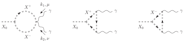
Figure 2: The genuine NLSM diagrams contributing to the $X_{0}\to\gamma\gamma$ process. The remaining diagrams are equivalent to the usual SM graphs and therefore are not shown.

After separating the NLSM new scalar contributions (${\cal A}_{\scriptscriptstyle\rm NL}$) from the fermionic (where we keep only the top contribution) and the vector-Goldstone-ghost ones (${\cal A}_{\scriptscriptstyle\rm f}$ and ${\cal A}_{\scriptscriptstyle\rm gauge}$ respectively), we get the following results

$${\cal A}_{\scriptscriptstyle\rm NL} = -\frac{4e^{2}}{\pi^{2}}\frac{1}{M_{X_{0}}^{2}M_{\scriptscriptstyle W}^{2}s_{W}^{2}v}\frac{1}{e^{2}v^{2}-4M_{\scriptscriptstyle W}^{2}s_{W}^{2}}\Big{[}M_{X_{0}}^{2}\Big{(}M_{\scriptscriptstyle W}^{2}s_{W}^{2}-\frac{e^{2}}{4}v^{2}\Big{)}^{2}-e^{2}M_{\scriptscriptstyle W}^{2}M_{X^{\pm}}^{2}s_{W}^{2}v^{2}\Big{]}$$

$$\times (k_{1}\cdot k_{2}\,g^{\mu\nu}-k_{1}^{\nu}k_{2}^{\mu})\epsilon^{*}_{\mu}(k_{1})\epsilon^{*}_{\nu}(k_{2})\left[1+2M_{X^{\pm}}^{2}C_{0}(0,0,M_{X_{0}}^{2},M_{X^{\pm}}^{2},M_{X^{\pm}}^{2},M_{X^{\pm}}^{2})\right],$$

$${\cal A}_{\scriptscriptstyle\rm f} = \frac{e^{3}}{\pi^{2}}\frac{m_{t}^{2}{\cal Y}}{M_{X_{0}}^{2}M_{\scriptscriptstyle W}s_{W}}(k_{1}\cdot k_{2}\,g^{\mu\nu}-k_{1}^{\nu}k_{2}^{\mu})\epsilon^{*}_{\mu}(k_{1})\epsilon^{*}_{\nu}(k_{2})$$

$$\times \left[-2+(M_{X_{0}}^{2}-4m_{t}^{2})C_{0}(0,0,M_{X_{0}}^{2},m_{t}^{2},m_{t}^{2},m_{t}^{2})\right],$$

$${\cal A}_{\scriptscriptstyle\rm gauge} = -\frac{e^{4}}{16\pi^{2}}\frac{v}{M_{X_{0}}^{2}M_{\scriptscriptstyle W}^{2}s_{W}^{2}}(k_{1}\cdot k_{2}\,g^{\mu\nu}-k_{1}^{\nu}k_{2}^{\mu})\epsilon^{*}_{\mu}(k_{1})\epsilon^{*}_{\nu}(k_{2})$$ (34)

$$\times \left[-M_{X_{0}}^{2}-6M_{\scriptscriptstyle W}^{2}+6(M_{X_{0}}^{2}-2M_{\scriptscriptstyle W}^{2})M_{\scriptscriptstyle W}^{2}C_{0}(0,0,M_{X_{0}}^{2},M_{\scriptscriptstyle W}^{2},M_{\scriptscriptstyle W}^{2},M_{\scriptscriptstyle W}^{2})\right].$$

In the formulas above $k_{1,2}$ are the momenta of the photons (with $2k_{1}\cdot k_{2}=M_{\scriptscriptstyle X_{0}}^{2}$) and $\epsilon$ represents the photon polarization vector; notice that the appearance of the common tensorial structure $k_{1}\cdot k_{2}\,g^{\mu\nu}-k_{1}^{\nu}k_{2}^{\mu}$ is dictated by gauge-invariance. Finally, for the particular kinematic configuration of this decay the Passarino-Veltman three-point function $C_{0}$ is known to be (see, e.g, Marciano:2011gm )

$$C_{0}(0,0,m^{2},M^{2},M^{2},M^{2})=-\frac{2}{m^{2}}f\left(\frac{4M^{2}}{m^{2}}\right)$$ (35)

where

$$f(\beta)=\left\{\begin{tabular}[]{ll}$\arcsin^{2}(\beta^{-\frac{1}{2}})$&\text{for $\beta\geq 1$}\\ $-\frac{1}{4}\Big{[}\ln\frac{1+\sqrt{1-\beta}}{1-\sqrt{1-\beta}}-i\pi\Big{]}^{2}$&\text{for $\beta<1$}\\ \end{tabular}\right.\vskip 6.0pt plus 2.0pt minus 2.0pt$$ (36)

It can be easily checked that setting $M_{\scriptscriptstyle W}=\frac{1}{2}gv$, $M_{\scriptscriptstyle X_{0}}=M_{h}$ (the Higgs mass) and ${\cal Y}=1$ the two amplitudes ${\cal A}_{\scriptscriptstyle\rm f}$ and ${\cal A}_{\scriptscriptstyle\rm gauge}$ reduce to their SM counterparts. Also notice that ${\cal A}_{\scriptscriptstyle\rm NL}$ diverges for $M_{\scriptscriptstyle W}=\frac{1}{2}gv$, which is equivalent to $A\rightarrow 0$. This corresponds to the singularity associated to the change in the number of degrees of freedom, since for $A\rightarrow 0$ the $\chi$’s become the Goldstone fields and therefore one must not add the amplitude ${\cal A}_{\scriptscriptstyle\rm NL}$, since the Goldstone loop is already included in ${\cal A}_{\scriptscriptstyle\rm gauge}$ [see Eq. (21)].

Next, in order to compare with the SM case let us construct the ratio

$$R=\frac{{\cal A}_{\scriptscriptstyle\rm NLSM}}{{\cal A}_{\scriptscriptstyle\rm SM-like}(a,c)},$$ (37)

where ${\cal A}_{\scriptscriptstyle\rm NLSM}={\cal A}_{\scriptscriptstyle\rm NL}+{\cal A}_{\scriptscriptstyle\rm f}+{\cal A}_{\scriptscriptstyle\rm gauge}$, while ${\cal A}_{\scriptscriptstyle\rm SM-like}(a,c)$ is a linear combination of the SM vector-Goldstone-ghost and fermionic contributions weighted, respectively, by two coefficients $a$ and $c$ which represent common rescaling factors with respect to the SM prediction for the Higgs couplings to vector bosons and fermions. The latter coefficients have been determined through fits to the LHC data Giardino:2012dp .

A comment is in order here. To carry out the fit to LHC data in a fully satisfactory way, one should make the comparison at the level of widths and cross sections. This is because, in addition to the dependence on the model parameters entering into the ratio $R$, one should also consider an extra dependence arising from the $gg\rightarrow X_{0}$ cross section. An estimate of such a dependence is left for a future study; the ensuing preliminary discussion only aims at estimating the impact arising from the additional NLSM terms in the $X_{0}\rightarrow\gamma\gamma$ amplitude.

According to Ref. Giardino:2012dp , one finds two possible scenarios that allow for an enhancement of the diphoton decay channel. The first scenario has the scalar coupling to fermions reduced with respect to the SM predictions and a somewhat enhanced Higgs boson couplings to vectors; the second scenario has the scalar coupling to fermions with opposite sign with respect to the SM prediction, as well as smaller couplings to the gauge bosons. The central values for these scenarios are roughly $(1.1,0.75)$ in the first case and $(0.8,-0.75)$ in the second case; clearly $(1,1)$ corresponds to the conventional SM case.

$\alpha(M_{\scriptscriptstyle X_{0}})$	$e$	$s_{\scriptscriptstyle W}^{2}$	$v$	$M_{\scriptscriptstyle X_{0}}$	$M_{\scriptscriptstyle W}$	$m_{t}$
$1/128$	$\sqrt{4\pi\alpha(M_{\scriptscriptstyle X_{0}})}$	0.23	$254$ GeV	$125.6$ GeV	80.385 GeV	173.5 GeV

Table 1: Input parameters for the calculation of the ratio $R$ of Eq. (37). The choice $\alpha(M_{\scriptscriptstyle X_{0}})\sim 1/128$ was taken from Degrassi:2003rw .

The strategy we adopt is then the following. By fixing the parameters $(a,c)$ to any of the values quoted for the three scenarios, one automatically fixes the normalization factor ${\cal A}_{\scriptscriptstyle\rm SM-like}(a,c)$. At this point we impose the condition $R=1$ and solve it in order to determine the corresponding value of the NLSM Yukawa coupling ${\cal Y}$.

The results of this procedure, taking as input parameters the ones summarized in Table 1, are shown in Fig. 3, where one can see that in any case the NLSM has the very distinctive signature of always requiring a negative Yukawa coupling between the top and the $X_{0}$ scalar to accommodate for the measured branching ratio in the diphoton channel.

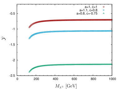
Figure 3: The NLSM Yukawa coupling needed for reproducing the scalar diphoton channel. The predicted Yukawa value is always negative.

IV Conclusions

The experimental verification of the Higgs mechanism is a two-step process. The first of these steps has been spectacularly completed by ATLAS and CMS with the discovery of a bosonic resonance at about $125$ GeV. The second step (and probably the most difficult one) crucially relies on the measurement of the new particle couplings and their comparison with the (very constrained) SM predictions for the Higgs boson. We are therefore on the verge of a very delicate turning point, in which the experimental data should be checked not only against the SM (and, implicitly, all its underlying assumptions) but also against all the available theoretical scenarios that predict deviation from it.

In this paper we have proposed a plain vanilla realization of one of these latter models, in the form of an electroweak SU(2)$\otimes$U(1) theory (dubbed NLSM) in which the gauge group is realized non-linearly, and the intermediate gauge bosons acquire their mass through the Stückelberg mechanism. Though non-renormalizable, the model is unitary and in addition the two simultaneous requirements of (i ) satisfying the WPC (which singles out uniquely the field theory Hopf algebra) while (ii ) being able to reproduce well-established experimental results (e.g, the absence of FCNCs) strongly constraint the form of the NLSM Lagrangian.

In this paper we have analyzed some peculiar features of the NLSM:

• When one tries to include scalar resonances, the minimum number of particles one can introduce in the NLSM is four corresponding to two neutral (one CP even and one CP odd) and two charged scalars: no scalar singlet is allowed. This fact alone singles out the NLSM w.r.t. two of the most popular SM extensions, namely the two Higgs-doublet model and the Minimal Supersymmetric Standard Model, both requiring, in their minimal realization, five scalars;

• To account for the (experimentally verified) suppression of the decay channel to VV w.r.t the $\gamma\gamma$, demands the inclusion of a SSB mechanism on top of the Stückelberg mechanism. However, contrary to the conventional case, in the NLSM the vev  $v$ gives mass only to the CP-even resonance $X_{0}$ while all masses of the remaining particles and their respective couplings are unaffected, a fact which can account for physics beyond the SM.

Thus the NLSM constructed here represents, to the best of our knowledge, the first example of a model in which a SSB mechanism exists that has nothing to do with the generation of fermions and gauge bosons masses.

As a warming-up exercise towards a phenomenological analysis, we have also performed a preliminary study of the $X_{0}\to\gamma\gamma$ decay channel and found that, in order to accommodate the ATLAS/CMS data, the NLSM CP-even scalar $X_{0}$ has always to couple to the top quark through a negative Yukawa coupling. And this is true even in the case in which the measured values would not ultimately deviate from the SM expected results.

While it is definitely too early to envisage in the LHC measurements any clear hint of deviations from the SM predictions for the candidate SM Higgs, one might reasonably expect that in all scenarios the comparison with the NLSM could be a very useful benchmark to pinpoint the Higgs mechanism as the actual mass generation mechanism chosen by Nature.

Appendix A Bleached Variables

One can form local SU(2)-invariant variables (bleached fields) as explained in Bettinelli:2008qn . The change of variables from the original to the bleached fields is invertible. Since the bleached variables are SU(2)-invariant, their hypercharge and electric charge coincide.

The SU(2) gauge fields $A_{\mu}=A_{a\mu}\frac{\tau_{a}}{2}$ and the $\rm U(1)_{\scriptscriptstyle Y}$ gauge field $B_{\mu}$ are combined into the bleached combination

$$w_{\mu} = w_{a\mu}\frac{\tau_{a}}{2}$$ (38)

$$= \Omega^{\dagger}gA_{\mu}\Omega+g^{\prime}\frac{\tau_{3}}{2}B_{\mu}+i\Omega^{\dagger}\partial_{\mu}\Omega.$$

One can easily verify that the above combination is invariant under the $\rm SU(2)_{\scriptscriptstyle L}$-gauge transformations

$$\Omega^{\prime} = U_{\scriptscriptstyle L}\Omega,$$ (39)

$$A^{\prime}_{\mu} = U_{\scriptscriptstyle L}A_{\mu}U_{\scriptscriptstyle L}^{\dagger}+\frac{i}{g}U_{\scriptscriptstyle L}\partial_{\mu}U_{\scriptscriptstyle L}^{\dagger}.$$ (40)

$w_{3\mu}$ represents the bleached counterpart of the $Z_{\mu}$ field, i.e.,

$$Z_{\mu}=\left.\frac{1}{\sqrt{g^{2}+g^{\prime 2}}}w_{3\mu}\right|_{\phi_{a}=0}=c_{\scriptscriptstyle W}A_{3\mu}+s_{\scriptscriptstyle W}B_{\mu}$$ (41)

where $s_{\scriptscriptstyle W}$ and $c_{\scriptscriptstyle W}$ are, respectively, the sine and cosine of the Weinberg angle, with

$$s_{\scriptscriptstyle W}=\frac{g^{\prime}}{\sqrt{g^{2}+g^{\prime 2}}};\qquad c_{\scriptscriptstyle W}=\frac{g}{\sqrt{g^{2}+g^{\prime 2}}},$$ (42)

and the photon $A_{\mu}$ is

$$A_{\mu}=-s_{\scriptscriptstyle W}A_{3\mu}+c_{\scriptscriptstyle W}B_{\mu}.$$ (43)

The bleached counterparts of the $W^{\pm}$ fields are instead given by

$$w^{\pm}_{\mu}=\frac{1}{\sqrt{2}}(w_{1\mu}\mp iw_{2\mu}).$$ (44)

For a generic $\rm SU(2)$ fermion doublet $L=\pmatrix{u\cr d}$, bleaching yields

$$\widetilde{L}=\Omega^{\dagger}L.$$ (45)

Finally, the bleached counterpart of the SU(2) scalar doublet $\chi=\chi_{0}+i\chi_{a}\tau_{a}$ is given by

$$\widetilde{\chi}=\Omega^{\dagger}\chi=\frac{1}{f}\left(\widetilde{\chi}_{0}+i\widetilde{\chi}_{a}\tau_{a}\right),$$ (46)

with

$$\widetilde{\chi}_{0} = \frac{1}{f}\left(\phi_{0}\chi_{0}+\phi_{a}\chi_{a}\right),$$

$$\widetilde{\chi}_{a} = \frac{1}{f}\left(\phi_{0}\chi_{a}-\chi_{0}\phi_{a}+\epsilon_{abc}\phi_{b}\chi_{c}\right).$$ (47)

This results in two neutral scalar fields, one CP-even ($\widetilde{\chi}_{0}$) and one CP-odd ($\widetilde{\chi}_{3}$), and two charged scalars $\widetilde{\chi}^{\pm}$, with

$$\widetilde{\chi}^{\pm}=\frac{1}{\sqrt{2}}\left(\widetilde{\chi}^{1}\mp i\widetilde{\chi}^{2}\right).$$ (48)

References

- (1) G. Aad et al. [ATLAS Collaboration], Phys. Lett. B [arXiv:1207.7214 [hep-ex]].
- (2) S. Chatrchyan et al. [CMS Collaboration], Phys. Lett. B [arXiv:1207.7235 [hep-ex]].
- (3) P. P. Giardino, K. Kannike, M. Raidal and A. Strumia, arXiv:1207.1347 [hep-ph].
- (4) J. Ellis and T. You, “Global Analysis of the Higgs Candidate with Mass 125 GeV”, arXiv:1207.1693 [hep-ph].
- (5) J. R. Espinosa, C. Grojean, M. Muhlleitner and M. Trott, “First Glimpses at Higgs’ face”, arXiv:1207.1717 [hep-ph].
- (6) F. Englert and R. Brout, Phys. Rev. Lett. 13, 321 (1964).
- (7) P. W. Higgs, Phys. Lett. 12, 132 (1964).
- (8) P. W. Higgs, Phys. Rev. Lett. 13, 508 (1964).
- (9) G. S. Guralnik, C. R. Hagen and T. W. B. Kibble, Phys. Rev. Lett. 13, 585 (1964).
- (10) E. C. G. Stückelberg, Helv. Phys. Helv. Acta 11 (1938), 299.
- (11) D. Bettinelli, R. Ferrari and A. Quadri, Int. J. Mod. Phys. A 24 (2009) 2639 [Erratum-ibid. A 27 (2012) 1292004] [arXiv:0807.3882 [hep-ph]].
- (12) D. Bettinelli, R. Ferrari and A. Quadri, Acta Phys. Polon. B 41 (2010) 597 [arXiv:0809.1994 [hep-th]].
- (13) D. Bettinelli, R. Ferrari and A. Quadri, Phys. Rev. D 77 (2008) 045021 [arXiv:0705.2339 [hep-th]].
- (14) D. Bettinelli, R. Ferrari and A. Quadri, Phys. Rev. D 79 (2009) 125028 [Erratum-ibid. D 85 (2012) 049903] [arXiv:0903.0281 [hep-th]].
- (15) R. Ferrari and A. Quadri, Int. J. Theor. Phys. 45 (2006) 2497 [hep-th/0506220].
- (16) R. Ferrari and A. Quadri, JHEP 0411 (2004) 019 [hep-th/0408168].
- (17) D. Bettinelli, R. Ferrari and A. Quadri, JHEP 0703 (2007) 065 [hep-th/0701212].
- (18) R. Ferrari, JHEP 0508 (2005) 048 [hep-th/0504023].
- (19) A. Quadri, Eur. Phys. J. C 70, 479 (2010) [arXiv:1007.4078 [hep-th]].
- (20) D. Bettinelli, R. Ferrari and A. Sanzeni, “Nonlinear Realization of the SU(5) Georgi-Glashow Model,” arXiv:1210.1486 [hep-ph].
- (21) D. A. Ross and M. J. G. Veltman, Nucl. Phys. B 95, 135 (1975).
- (22) G. F. Giudice, C. Grojean, A. Pomarol and R. Rattazzi, JHEP 0706 (2007) 045 [hep-ph/0703164].
- (23) R. Contino, C. Grojean, M. Moretti, F. Piccinini and R. Rattazzi, JHEP 1005 (2010) 089 [arXiv:1002.1011 [hep-ph]].
- (24) R. Grober and M. Muhlleitner, JHEP 1106 (2011) 020 [arXiv:1012.1562 [hep-ph]].
- (25) W. Buchmuller and D. Wyler, Nucl. Phys. B 268 (1986) 621.
- (26) A. Connes and D. Kreimer, Commun. Math. Phys. 210, 249 (2000) [hep-th/9912092].
- (27) A. Connes and D. Kreimer, Commun. Math. Phys. 216, 215 (2001) [hep-th/0003188].
- (28) K. Ebrahimi-Fard and F. Patras, Annales Henri Poincare 11 (2010) 943 [arXiv:1003.1679 [math-ph]].
- (29) S. L. Glashow, J. Iliopoulos and L. Maiani, Phys. Rev. D 2, 1285 (1970).
- (30) S. Schael et al. [ALEPH and DELPHI and L3 and OPAL and SLD and LEP Electroweak Working Group and SLD Electroweak Group and SLD Heavy Flavour Group Collaborations], Phys. Rept. 427, 257 (2006) [hep-ex/0509008].
- (31) LHC Higgs Cross Section Working Group, A. David, A. Denner, M. Duehrssen, M. Grazzini, C. Grojean, G. Passarino and M. Schumacher et al., “LHC HXSWG interim recommendations to explore the coupling structure of a Higgs-like particle”, arXiv:1209.0040 [hep-ph].
- (32) G. Passarino, “NLO Inspired Effective Lagrangians for Higgs Physics,” arXiv:1209.5538 [hep-ph].
- (33) A. Denner, Fortsch. Phys. 41 (1993) 307 [arXiv:0709.1075 [hep-ph]].
- (34) W. J. Marciano, C. Zhang and S. Willenbrock, Phys. Rev. D 85, 013002 (2012) [arXiv:1109.5304 [hep-ph]].
- (35) G. Degrassi and A. Vicini, Phys. Rev. D 69 (2004) 073007 [hep-ph/0307122].