Controlling crystal self-assembly using a real-time feedback scheme

Abstract

We simulate crystallisation of hard spheres with short-ranged attractive potentials, as a model self-assembling system. Using measurements of correlation and response functions, we develop a method whereby the interaction parameters between the particles are automatically tuned during the assembly process, in order to obtain high-quality crystals and avoid kinetic traps. The method we use is independent of the details of the interaction potential and of the structure of the final crystal – we propose that it can be applied to a wide range of self-assembling systems.

I introduction

In self-assembly white02review ; sol07 , simple components like colloids and biomolecules come together spontaneously, forming ordered structures such as viral capsids hagan06 ; rap08 , crystals leunissen05 ; Hynn2007 ; sear07 ; nyk08 ; chen11 ; romano11 ; klotsa11 , or DNA origami rothemund06 . Recent developments in self-assembly include the experimental synthesis of particles with specific controllable interactions nyk08 ; chen11 ; pawar09 ; sac10 ; kraft12 , as well as theoretical and computational demonstrations of the ordered phases that such particles can form wilber09 ; akbari09 ; romano11 ; martinez11 . However, even when ordered states are stable, appearance of disordered aggregates often frustrates the dynamical self-assembly process. As a result, effective assembly typically involves microscopic reversibility: if bonds are both made and broken during self-assembly then defects are annealed naturally, producing an ordered final state white02 ; hagan06 ; rap08 ; whitelam09 ; grant11 ; klotsa11 . The twin requirements of a stable ordered structure and the reversibility of bonding usually mean that assembly is effective only when interaction parameters are tuned to lie within a narrow ‘optimal’ range hagan06 ; whitelam09 ; klotsa11 ; jankowski11 ; grant11 .

In some experiments and in simulations, interactions between particles can be manipulated during the assembly process, in order to optimize assembly conditions and facilitate the kinetics. For example, a slow cooling process is used in hierarchical assembly of DNA origami rothemund06 , and light exposure in repeated pulses may allow control of nanoparticle aggregation klajn07 ; jha12 . However, such protocols have, so far, been largely empirical. Given a desired ordered structure and a particle with controllable interactions, it is far from clear how these interactions should change in time in order to achieve the best self-assembly. One might expect that gradually increasing the interaction strength would allow the product structure to form smoothly and reversibly, as in Ref rothemund06, . But there is little evidence that this scheme is optimal for assembling ordered structures quickly and reliably.

In this paper, we develop a method for automatically choosing protocols (series of steps) by which interactions between particles should be manipulated in order to achieve the best assembled products in the most efficient way. We do this by measuring the reversibility of particle bonding, as assembly is taking place. The resulting cycle of measurements and changes in interaction strength forms an elementary feedback loop. Using computer simulations, we show that (i) our feedback scheme quickly locates interaction parameters for which assembly is effective, and (ii) it forms higher-quality crystals than assembly with fixed (time-independent) interactions. We also find that the protocols that give best assembly are not gradual cooling schemes, and we discuss the reasons for this observation. The feedback scheme does not rely in any way on the structure of the ordered (crystal) state – we expect that it can be applied to other self-assembly processes with minimal modification. Our results provide a proof of concept for this method, which is efficient in automatically finding effective assembly protocols, and avoiding metastable disordered states.

Currently, this method is best-suited to implementation in computer simulation, where interactions between particles can easily be controlled, and measurements of reversibility are relatively simple to make. We emphasise that our computer simulations give dynamically-realistic descriptions of the self-assembly process, so if a given set of time-dependent interactions is effective in simulation, we would expect them to be effective in experiment too.

II Model

We consider crystallisation of hard spheres with short-ranged attractive isotropic interactions, as a model self-assembly process. This system might represent a suspension of colloidal particles interacting through depletion forces whitelam09 ; fortini08 ; klotsa11 , or a solution of protein molecules used in protein crystallisation frenkel97 ; rosenbaum96 ; rosenbaum99 ; sear07 .

We take $N=10,000$ spherical particles with hard cores of diameter $\sigma$, at volume fraction $\phi=0.04$ and temperature $T$. The particles interact through a pair potential $U(r)$ which is a square well of depth $\varepsilon_{\mathrm{b}}$ and range $\xi=0.1\sigma$. Phase diagrams for such systems have been calculated (for example) by Liu et al. liu05 , showing a fluid-crystal phase coexistence regime that contains a metastable fluid-fluid critical point. The square well potential that we use is a coarse-grained representation of attractive interactions: in colloidal suspensions or protein solutions, it accounts for the effects of depletion interactions, hydrophobic association and/or screened electrostatic charges. The model is therefore somewhat schematic, but we build on the observation rosenbaum96 ; rosenbaum99 ; noro2000 that for systems with short-ranged attractions, the shape of the potential $U(r)$ is relatively unimportant, with the behaviour being largely dictated by the (reduced) second virial coefficient. Thus we expect our main findings to depend only weakly on the shape of this potential noro2000 ; liu05 .

To describe the motion of particles dispersed in a solvent, we use overdamped Langevin dynamics. Particles have (bare) diffusion constant $D_{0}$ and we define a time unit $\tau_{0}=\sigma^{2}/D_{0}$, of the order of a Brownian time. Our model therefore neglects hydrodynamic effects arising from the solvent, and may underestimate the rates of diffusion for large clusters of colloidal particles spaeth11 . However, Langevin dynamics do capture the essential physical processes at work in self-assembly hagan06 ; whitelam09 ; wilber09 ; romano11 ; klotsa11 : reversible bonding, nucleation of ordered phases, the possibility for kinetic trapping, and Ostwald ripening. We therefore use this method for computational convenience and for ease of comparison with other studies whitelam09 ; klotsa11 . We do not expect our neglect of hydrodynamic effects to have strong effects on the competition between reversible bonding and kinetic trapping, which will be our main focus in what follows. We return to possible hydrodynamic effects in Sec. V.2 below.

To simulate the Langevin dynamics of the system, we use single particle Monte Carlo (MC) moves. Full details of the computational scheme are given in in Ref. klotsa11, : we note that the time unit used in this work is $\tau_{0}\approx 270$ MC sweeps. As discussed in Refs. whitelam09, ; whitelam11-molsim, ; sanz10-mc-bd, , single particle MC moves give an accurate representation of the Langevin dynamics, as long as the step size is sufficiently small. If the step size is too large, it is possible that rejected MC moves act to reduce the diffusion of large clusters, but the results of Ref. whitelam09, show that this has little effect on the assembly pathway or the final product, in a very similar crystallising system. The initial conditions of all simulations are taken from equilibrated hard sphere systems at the relevant volume fraction.

In a preceding paper [klotsa11, ] we reported simulations of the model system described here, with fixed (time-independent) interaction parameters. We found that for times up to $10^{4}\tau_{0}$, appreciable crystallization takes place only for $2.3<\varepsilon_{\mathrm{b}}/T<3.0$, with $\varepsilon_{\mathrm{b}}/T=2.5$ the optimum value. For $\varepsilon_{\mathrm{b}}/T<2.0$ the system is in the stable fluid phase and does not assemble. For $\varepsilon_{\mathrm{b}}/T>4.0$ the system makes bonds that are too strong and gets kinetically trapped (see also the phase diagram sketched in Fig. 1 of Ref. klotsa11, ).

Here, we perform two kinds of computer simulation: (i) ‘No-Feed’ protocol. The interactions are fixed and time-independent (as in Ref. klotsa11, ). We focus on bond strengths close to the optimal value $\varepsilon_{\mathrm{b}}/T$=2.5. (ii) ‘With-Feed’ protocol. The interactions change in time according to the feedback scheme. The initial bond strength $\varepsilon_{\mathrm{b}}^{\mathrm{init}}$ is a free parameter: the aim of the feedback scheme is that it should tune the system into a good-assembly regime, independently of $\varepsilon_{\mathrm{b}}^{\mathrm{init}}$. We present three representative cases, $\varepsilon_{\mathrm{b}}^{\mathrm{init}}/T=1.0,2.5,7.0$. If these bond strengths were used in ‘No-feed’ simulations, they would lead to no assembly, near-optimal assembly, and kinetic trapping, respectively.

III Feedback scheme

III.1 Fluctuation-dissipation theorem

Previous studies on glasses crisanti03 ; kurchan05 ; baiesi09 , self-assembling systems jack07 ; klotsa11 ; grant11pre and gels russo10 have used out of equilibrium correlation and response functions to characterise dynamical behaviour baiesi09 ; seifert10 . Our hypothesis jack07 is that by focussing on the dynamics of an evolving system, without knowledge of its structure, we can quantify how reversible the system is and therefore predict whether it is prone to get kinetically trapped or not.

In practice, we perturb the dynamics of the system, writing the energy as $E=\frac{1}{2}\sum_{p}(1+h_{p})E_{p}$ where $E_{p}=\sum_{p^{\prime}}U(|\bm{r}_{p}-\bm{r}_{p^{\prime}}|)$ is the energy of particle $p$ and $h_{p}$ is a perturbing field applied to that particle. The total energy in the presence of the perturbation is therefore $E=\sum_{pp^{\prime}}(1+\frac{1}{2}(h_{p}+h_{p^{\prime}}))U(|\bm{r}_{p}-\bm{r}_{p^{\prime}}|)$, and we emphasise that the dynamics obeys detailed balance with respect to this energy function whenever the perturbation is imposed. The perturbation is switched on at time $t_{w}$. The energy autocorrelation function and the response function for that perturbation are (respectively)

$$C(t,t_{\mathrm{w}}) =\langle E_{p}(t)E_{p}(t_{\mathrm{w}})\rangle-\langle E_{p}(t)\rangle\langle E_{p}(t_{\mathrm{w}})\rangle$$ (1)

$$\chi(t,t_{\mathrm{w}}) =\frac{T}{2}\frac{\partial}{\partial h_{p}}\langle E_{p}(t)\rangle.$$ (2)

We make use of the fact that at equilibrium the system is by definition reversible in time and the relation between the correlation and response functions is given by the fluctuation-dissipation theorem (FDT) $\chi^{\mathrm{eqm}}(t,t_{\mathrm{w}})=C^{\mathrm{eqm}}(t,t)-C^{\mathrm{eqm}}(t,t_{\mathrm{w}})$. (For the specific observables considered here, a proof of this FDT was given in Ref. klotsa11, .) In an assembling system, we can therefore evaluate how much the relation between $C(t,t_{w})$ and $\chi(t,t_{w})$ deviates from the equilibrium FDT relation. We find three broad classes of behaviour: (i) No deviation from FDT. In this case the system is truly reversible and already at equilibrium. (ii) Large deviation. The system is highly irreversible and thus likely to get kinetically trapped. (iii) Small but finite deviation. The system is reversible at short timescales and becomes irreversible at longer timescales. Here, the difference between ‘small’ and ‘large’ deviations may be calculated from dimensionless parameters that lie between $0$ and $1$: see below. We have shown that the case (iii) above is typically correlated with optimal self-assembly jack07 ; klotsa11 ; grant11pre . The reason is that small deviations from FDT behaviour indicate the right balance between the microscopically reversible particle bonding and the macroscopically irreversible self-assembly grant11pre – which are the two requirements for effective assembly.

In the present paper, the feedback scheme is used to evaluate which of the three options best characterises the dynamics of the system under investigation, and to dynamically tune the interaction strength between the particles accordingly, until the dynamics is consistent with case (iii).

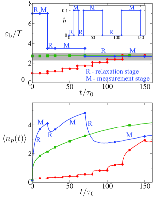
Figure 1: Operation of the feedback loop on short time scales for three ‘With-Feed’ simulations with different initial bond strengths $\varepsilon_{\mathrm{b}}^{\mathrm{init}}$. (Top) Time-dependence of the bond strength $\varepsilon_{\mathrm{b}}$. Measurement and relaxation stages are indicated for the run with $\varepsilon_{\mathrm{b}}^{\mathrm{init}}/T=7.0$. The shaded region indicates where ‘No-Feed’ simulations found appreciable crystallisation. The inset shows the time-dependence of the perturbation strength $\tilde{h}$ for the run with $\varepsilon_{\mathrm{b}}^{\mathrm{init}}/T=7.0$. (Bottom) Average number of bonds per particle $\langle n_{p}(t)\rangle=\frac{\langle E_{p}(t)\rangle}{(-\varepsilon_{\mathrm{b}})}$.

III.2 Implementation of feedback scheme

The feedback scheme consists of alternating ‘measurement’ and ‘relaxation’ stages, as shown in Fig. 1. We describe the main points here: a full description of the implementation of the scheme is given in the Appendix. In measurement stages, we perturb the particles with fields $h_{p}$ (inset to Fig.1) and we measure correlation and response functions. The strength of the perturbation is given by a dimensionless parameter $\tilde{h}$: see Appendix. At the end of each measurement stage, the bond strength $\varepsilon_{\mathrm{b}}$ is updated, according to the measurements that have been made. Each measurement stage is followed by a relaxation stage during which $h_{p}=0$; after this relaxation stage the next measurement stage begins.

If the $i$th measurement stage begins at time $t_{i}$, it is convenient to normalise correlation and response functions as $\tilde{C}(t,t_{i})=C(t,t_{i})/C(t,t)$ and $\tilde{\chi}(t,t_{i})=\chi(t,t_{i})/C(t,t)$. We define the ratio

$$\tilde{X}(t,t_{i})=\frac{\chi(t,t_{i})}{C(t,t)-C(t,t_{i})}.$$ (3)

For a reversible (equilibrated) system, $\tilde{X}=1$, in accordance with FDT; for irreversible aggregation we typically find $\tilde{X}\approx 0$. This ratio provides a dimensionless measurement of the deviation from reversibility: we expect that for optimal assembly $\tilde{X}$ is close but not equal to 1, as in Refs jack07, ; klotsa11, ; grant11pre, . We note that $\tilde{X}$ differs from the fluctuation-dissipation ratio crisanti03 (FDR), which would be an alternative dimensionless measurement. However, the FDR involves a ratio of derivatives of $\chi$ and $C$, while $\tilde{X}$ is obtained directly from the values of these functions and is therefore easier to calculate in simulation. Our previous work jack07 ; klotsa11 ; grant11pre indicates that both the FDR and $\tilde{X}$ are well-correlated with the reversibility of self-assembly.

At the end of each measurement stage, the feedback scheme updates the bond strength $\varepsilon_{\mathrm{b}}$, depending on $\tilde{X}$. We use the simple update rule

$$\varepsilon_{\mathrm{b}}^{\mathrm{new}}=\varepsilon_{\mathrm{b}}^{\mathrm{old}}\left[1+\frac{\alpha}{\gamma_{i}}(\tilde{X}-X_{0})\right].$$ (4)

Here $X_{0}$ is the target for the response strength $\tilde{X}$. We take $X_{0}=0.8$, which makes concrete the requirement in Sec. III.1 that deviations from FDT should be “small but finite”. Also, $\alpha=1$ determines the sensitivity of the feedback loop, and $\gamma_{i}$ is a damping parameter. We take $\gamma_{1}=1$ for the first measurement phase; at the end of subsequent measurement phases then $\gamma_{i}$ is increased by $1$ if the response $\tilde{X}$ is within a tolerance $\delta X$ of $X_{0}$. We take $\delta X=0.1$. Further information on the choices of the parameters $(X_{0},\alpha,\delta X)$ are given in the Appendix.

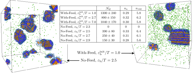
Figure 2: Configurations from ‘No-feed’ (left) and ‘With-feed’ (right) simulations at $t=10^{4}\tau_{0}$, and averaged measures of crystallinity at this time. In the snapshots, particles in fcc/hcp environments are coloured orange/purple. Particles in other environments are rendered at half their actual diameter for visual clarity. The data in the table are averaged either over 8 independent simulations (‘No-Feed’) or over the $M=8$ systems associated with single ‘With-Feed’ simulations (see Appendix). For $\mathcal{N}_{Q}$, we show the standard errors on these averages, as an indicator of the numerical uncertainty. For $n_{\rm x}$ and $n_{142}$, these errors are small: no larger than $0.02$ and $0.2$ respectively. The uncertainties on $\mathcal{N}_{Q}$ are significant but it is clear that ‘With-feed’ simulations form ‘higher-quality’ crystals with larger close-packed domains.

To complete the description of the feedback loop, we specify the durations of measurement and relaxation stages: that is, the time over which the perturbation $h_{p}$ is applied, and the time allowed between successive perturbations. These are determined self-consistently: for measurements of reversibility of bonding to be useful, they must be made on appropriate time scales, and these may not be known a priori. The $i$th measurement stage ends when $t$ is large enough that either $\tilde{C}(t,t_{i})<C^{*}$ or $\tilde{X}(t,t_{i})<X^{*}$, where $C^{*}=0.3$ and $X^{*}=0.6$ are parameters associated with the feedback scheme (see Section V.1 below and the Appendix for more details).

IV Results

In this section we present our simulation results, considering both systems with the feedback scheme on (With-Feed) and with the feedback scheme off (No-Feed).

IV.1 Feedback loop

The behaviour during the first few stages of the feedback loop is summarised in Fig. 1. The first key result of this paper is that for a range of initial bond strengths $\varepsilon_{\mathrm{b}}^{\mathrm{init}}$, the feedback scheme quickly tunes the interaction strength $\varepsilon_{\mathrm{b}}/T$ into the (narrow) range where assembly is effective.

More specifically, for $\varepsilon_{\mathrm{b}}^{\mathrm{init}}/T=7.0$, the system is vulnerable to kinetic trapping in disordered states, but the feedback loop automatically reduces the bond strength to avoid this problem. Similarly for $\varepsilon_{\mathrm{b}}^{\mathrm{init}}/T=1.0$, the system will never assemble if the bond strength is held constant, but the feedback scheme increases $\varepsilon_{\mathrm{b}}$ in order to achieve assembly. Finally, for $\varepsilon_{\mathrm{b}}^{\mathrm{init}}/T=2.5$ the feedback loop can recognize that the interaction strength is optimal and does not try to alter the value of $\varepsilon_{\mathrm{b}}$. This demonstrates the idea that automated real-time control of interaction parameters can be used to promote effective self-assembly.

IV.2 Crystal structure

To assess the effectiveness of this scheme, we analyse the crystals that are assembled within the No-Feed and With-Feed protocols on the relatively long time scale $t=10^{4}\tau_{0}$. Results are summarised in Fig. 2. Results for longer times are qualitatively similar, although there is some slow growth in crystalline order as coarsening (Ostwald ripening) takes place.

We measure the crystallinity of the assembled system using both local packing and long-ranged orientational order. Local packing is examined using a common neighbour analysis (CNA) hon87 . The CNA assigns a 4-digit signature to each bonded pair of particles in the system. Bonds with ‘1421’ or ‘1422’ signatures are characteristic of close-packed crystals: we measure the mean number of such bonds per particle $n_{142}$, as in Ref. klotsa11, . If every particle is inside a perfect crystal then $n_{142}=12$. However, for the finite systems considered in simulation we always find smaller values of $n_{142}$: this is partly because many particles will be on the surfaces of crystalline clusters, and partly because the system also contains free monomer particles, and crystals also contain defects. We also use the CNA to identify particles whose local environment is consistent with face-centred cubic (fcc) or hexagonal close-packed (hcp) order. (Fcc particles have 12 bonds with ‘1422’ signatures while hcp particles have 6 bonds with ‘1421’ signatures and 6 with ‘1422’.) If the number of hcp (fcc) particles is $N_{\mathrm{hcp}}$ ($N_{\mathrm{fcc}}$) then we define the fraction of particles in perfectly crystalline environments as $n_{\mathrm{x}}=(N_{\mathrm{hcp}}+N_{\mathrm{fcc}})/N$. The maximal possible value for $n_{\mathrm{x}}$ is unity, but the presence of surface particles, free monomers and crystal defects all act to reduce this.

The table in Fig. 2 shows that the parameters $n_{142}$ and $n_{\mathrm{x}}$ are comparable between the With-Feed protocol (for initial bond strengths $1<\varepsilon_{\mathrm{b}}^{\mathrm{init}}/T<7$) and the No-Feed protocol (for the narrower ‘optimal’ range of bond strengths $2.5\leq\varepsilon_{\mathrm{b}}<2.9$). Around $30\%$ of particles end the simulation in bulk-crystalline environments. For these system sizes and densities, multiple nucleation events occur in all simulations, resulting in several ordered clusters per simulation. The ‘maximal yield’ of $30\%$ reflects the fact that particles on the surfaces of the clusters are never classed as crystalline, since they have fewer than 12 bonds.

Fig. 2 also shows snapshots of final configurations where hcp and fcc particles are highlighted: in the example shown, the ‘With-feed’ scheme has produced a close-packed crystal of around $4400$ particles. Other small crystalline clusters are also visible as a result of multiple nucleation. Other runs under the same conditions yield similar numbers of crystallites of similar sizes, although there is significant variation due to the stochastic nature of nucleation events. We emphasise that the large cluster that resulted from the With-Feed protocol is a close-packed crystal, albeit with random stacking of fcc/hcp planes. On the other hand, the ‘No-Feed’ simulations give some clusters where five-fold packing defects are apparent, presumably due to growth around a critical nucleus that lacks the symmetry of the crystal.

To analyse the larger scale order in the assembled crystallites and the presence of packing defects, we also measure the typical size of crystalline domains in the system using bond-order parameters. As in Refs. tenwolde95, ; fortini08, , let $\vec{q}_{6}(p)$ consist of the projection of the bonds of particle $i$ onto the spherical harmonics with $l=6$, normalised so that $\vec{q}_{6}(p)^{*}\cdot\vec{q}_{6}(p)=1$. Then, if $\vec{Q}=\sum_{p=1}^{N}\vec{q}_{6}(p)$ then $\mathcal{N}_{Q}=N^{-1}\langle\vec{Q}^{*}\cdot\vec{Q}\rangle$ is an estimate of the typical crystalline domain size. (To see this, we assume that $\vec{q}_{6}(p)^{*}\cdot\vec{q}_{6}(p^{\prime})\approx 1$ if particles $p$ and $p^{\prime}$ belong to the same domain, with $\vec{q}_{6}(p)^{*}\cdot\vec{q}_{6}(p^{\prime})\approx 0$ otherwise.) Of course, systems contain a distribution of domain sizes: the quantity $\mathcal{N}_{Q}$ gives equal weight to each particle, so large clusters have the largest contributions to $\mathcal{N}_{Q}$. Since equal weight is given to each particle, this measure of crystalline domain size is appropriate for measuring the yield of the crystallisation process.

Consistent with the snaphots in Fig. 2, the numerical results for $\mathcal{N}_{Q}$ in the associated table show that the ‘With-feed’ protocol results in significantly larger crystalline domains, compared to its ‘No-feed’ counterpart. There are differences in crystalline yield between different ‘With-Feed’ runs, coming partly from the choice of initial bond strength and partly from fluctuations of $C(t,t_{i})$ and $\chi(t,t_{i})$ in the measurement stages. However, the trends shown here are robust to these differences.

In evaluating the effectiveness of crystal self-assembly, we use $\mathcal{N}_{Q}$ as our main ‘figure-of-merit’, since applications of self-assembled crystals in photonics or X-ray diffraction both require well-developed Bragg resonances and hence large ordered domains. The ‘With-feed’ protocol produces larger values of $\mathcal{N}_{Q}$ than the ‘No-feed’ simulations – we conclude that the feedback scheme does facilitate crystallisation. This is our second key result, demonstrating explicitly how automated changes in time-dependent interaction parameters can be used to aid self-assembly.

V Discussion

The effectiveness of the feedback scheme relies on two central assumptions: (i) that correlation and response measurements can be used to obtain useful information about the reversibility of assembly, and (ii) that tuning the reversibility of assembly is effective in optimizing the self-assembly process. Here we discuss these two assumptions in more detail.

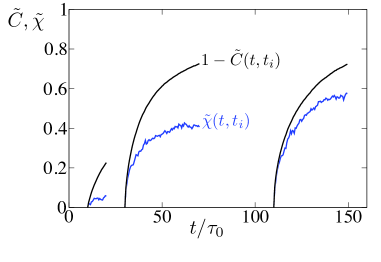
Figure 3: Behaviour of the correlation and response functions for a ‘With-Feed’ simulation with $\varepsilon_{\mathrm{b}}^{\mathrm{init}}/T=7.0$. (Other data for the same run was shown in Fig. 1). We show $1-\tilde{C}(t,t_{i})$ and $\tilde{\chi}(t,t_{i})$ for the first three iterations of the feedback loop. The responses $\tilde{\chi}(t,t_{i})$ are quite small when compared to $1-\tilde{C}(t,t_{i})$, indicating that irreversible bonding is taking place, and the system is vulnerable to kinetic trapping. As a result, the feedback loop acts to reduce the bond strength $\varepsilon_{\mathrm{b}}$ (see Fig. 1).

V.1 Duration of measurement and relaxation stages

For effective operation of our feedback scheme, measurements of reversibility of bonding during assembly must be made on time scales where significant bond-making and bond-breaking has taken place. These time scales are not known a priori: they depend on the particle interactions and they also change significantly during the assembly process. Hence, within the feedback scheme, we determine the durations of the measurement phases adaptively, using information contained in the correlation-response measurements themselves.

To illustrate this, consider Fig. 3, where the behaviour of $\tilde{C}(t,t_{i})$ and $\tilde{\chi}(t,t_{i})$ are shown for one of the ‘With-Feed’ simulations from Fig. 1. The functions $1-\tilde{C}(t,t_{i})$ and $\tilde{\chi}(t,t_{i})$ would coincide at equilibrium: their ratio is equal to $\tilde{X}$. In the first measurement stage, the bonds between particles are strong and the bonding almost irreversible – thus, $\tilde{\chi}$ is small and the ratio $\tilde{X}$ is much less than its cutoff $X^{*}$. As a result, the measurement stage is quickly terminated and the bond strength reduced. In the second and third measurement stages, the responses are larger, indicating that bonding is more reversible. These stages terminate when $\tilde{C}$ has fallen to $C^{*}$, indicating that the system has decorrelated significantly from its state at time $t_{i}$: by fixing a value for $C^{*}$ we ensure that different measurements of reversibility can be compared on an equal footing even when the absolute time scales for bonding and unbonding are changing. The duration of each relaxation stage is chosen to be equal to the previous measurement stage. (The only exception is the initial stage of the feedback loop which is a relaxation stage. This stage is included because making correlation-response measurements immediately after initialization of the system can be sensitive to transient behaviour that depends mostly on the initial conditions used, and is not necessarily correlated with the effectiveness of self-assembly. This initial relaxation stage has duration $10\tau_{0}$ which is sufficient time for initial transients to relax.)

We emphasise that the durations of the 3 measurement stages in Fig. 3 vary significantly. On longer time scales, this variation is even stronger, with the duration tending to increase as the system assembles. We also investigated schemes where the durations of measurement stages were fixed a priori, but these were less effective. Allowing these durations to vary within the scheme does add some complexity, but it does mean that no initial assumption is required as to the relevant time scale for measuring reversibility. We argue that this will aid implementation of the scheme in other self-assembling systems where the relevant time scales may not be known. Further information about the parameters $C^{*},X^{*}$ associated with the method is given in the Appendix – we expect the effectiveness of the feedback loop to depend weakly on these parameters.

V.2 Time-dependent assembly within feedback scheme

Figure 4: Behaviour of bond strength $\varepsilon_{\mathrm{b}}$ at long times, for the ‘With-Feed’ simulations of Fig. 1. The symbols and colors indicate the values of $\varepsilon_{\mathrm{b}}^{\mathrm{init}}$, which are the same as those in Fig. 1. The dashed line shows the ‘No-feed’ protocol that gave the best yield.

We have emphasised that the feedback loop is designed to exploit the reversibility of bonding in order to promote assembly. Here we discuss the time-dependent protocols that are selected by the feedback loop, which result in the good assembly shown in Fig. 2. We show these protocols in Fig. 4. On short time scales, the feedback scheme adjusts the system to have stronger bonds than the best No-Feed protocol, but on longer time scales the feedback mechanism reduces the bond strength. We note that the With-Feed scheme acts to optimise the reversibility of particle bonding: it is not obvious a priori that this approach of weakening bonds on long times should be effective in optimising either reversibility or assembly. In this sense, the ‘With-feed’ scheme is effective in arriving at non-trivial dynamical approaches for manipulating particle interactions.

Inspection of the assembly trajectories shows that for the bond strengths shown in Fig. 4, the short-time physics ($t\lesssim 100\tau_{0}$) is dominated by nucleation, while the behaviour on longer times is that of Ostwald ripening, with smaller clusters shrinking and larger ones growing. In this case, the With-Feed protocol leads naturally to a scheme where the bonds are initially strong, promoting nucleation; on later time scales the bonds are weaker, which promotes rapid Ostwald ripening (this is a thermally activated process in these systems, proceeding faster when bonds are weaker).

The weakening of bonds at long times in the feedback process arises due to properties of correlation and response functions during coarsening crisanti03 . Briefly, the coarsening of large crystalline clusters depends on their macroscopic properties (curvature and surface tension), so applying the perturbation $h_{p}$ does not affect whether the cluster containing particle $p$ should grow or shrink. In this sense, coarsening is an irreversible process. As a result, the response $\chi$ is small in the long-time (coarsening) regime, and the With-Feed protocol pushes the system to increasingly weak bonds. For very long times, it is possible that the With-Feed protocol may reduce $\varepsilon_{\mathrm{b}}$ so far that the bonds become too weak and the clusters disintegrate. We did not observe this, although we do find a similar effect when the damping term $\gamma_{i}$ is not included in (4). These possibilities should be considered when applying this scheme to other systems. For example, it may be useful in some systems to operate the feedback scheme only during early and intermediate stages of assembly, and to revert to a ‘No-feed’ method on very long times.

In this discussion of Ostwald ripening, it is also worth recalling the neglect of hydrodynamic effects in the simulation model being used, and the use of single particle MC moves in implementing the dynamics. Both these choices spaeth11 ; whitelam11-molsim act to reduce the diffusion of large clusters of particles. This favours the Ostwald ripening mechanism for assembly, compared with the process by which diffusing clusters collide and fuse. However, in evaluating the ‘With-feed’ scheme presented here, we emphasise that we are comparing it with a ‘No-feed’ scheme that uses the same model and simulation methods. So the improvement obtained by allowing time-dependent interactions is significant for this particular model. If the diffusion of large clusters were faster within the model (perhaps due to hydrodynamic effects), both the ‘No-feed’ and the ‘With-feed’ results would change. However, assuming that the link between reversible bonding and effective assembly is maintained, we would expect the feedback scheme presented here to vary the interaction strength so as to facilitate effective self-assembly in that case too. This hypothesis remains to be tested, as does the effectiveness of the feedback scheme in optimising assembly in other systems.

VI Outlook

To conclude, we have introduced an automated method for tuning interaction parameters during self-assembly, so as to avoid kinetic trapping and promote the formation of ordered structures. We have demonstrated in computer simulation that this method produces high-quality crystals, and we have emphasised that it can be generalised straightforwardly to other assembling systems. There is also potential for applications in experiments: attractions between colloidal particles can now be manipulated in real-time alsayed04 ; klajn07 ; hertlein08 ; elsner09 ; savage09 ; bonn09 ; taylor12 , and correlation-response measurements have also been made bonn07a ; oukris10 ; ruocco10 . We hope that the potential for automated self-assembly using real-time feedback will stimulate further studies in this area.

One direction that might be promising in computer simulation is to consider feedback schemes that do not rely on correlation-response measurements, but use other observables to tune assembly protocols. For example, one might use a structural measure within the feedback loop, to promote assembly. It would be possible to might make interactions stronger when there are too few bonds in the system, and weaken interactions if there are too many non-crystalline bonds. We have not investigated this approach so far, because it relies on the pathway to the ordered state being known a priori: this is not the case in viral capsid assembly hagan06 ; jack07 and there are many examples of non-trivial pathways in crystal nucleation too frenkel97 ; whitelam2010 . In those cases, the structural approach to optimising assembly becomes very hard to implement. Instead, we have chosen to concentrate specifically on the kinetics of binding and unbinding events, aiming to avoid kinetic trapping, but leaving the system free to explore all pathways towards the assembled state. A similar consideration applies to systems with several possible ordered states, such as crystal polymorphs. The approach that we have described does not select for any specific polymorph: it allows the system to form whatever ordered state it prefers. It would be interesting to explore polymorph selection within this kind of scheme, but we defer such issues to later publications.

Appendix A Implementation of feedback loop

A.1 Measurement of response functions

In general, accurate estimation of the response function $\chi(t,t_{i})$ requires good statistics, and our implementation of the feedback loop is designed to achieve this. We emphasise that while accurate estimation of $\chi$ does require some computational overhead, the usual alternative is to perform many ‘No-feed’ simulations over a range of $\varepsilon_{\mathrm{b}}$, in order to locate the good-assembly regime. That approach also requires significant CPU time: by using a feedback scheme, we focus the computational effort on the parameter range in which assembly is most effective, and on the potential benefits of using time-dependent interactions in self-assembly.

We note that $\chi(t,t_{i})$ is defined in terms of the response of a single representative particle. To ensure that information from all particles is used as efficiently as possible to estimate $\chi(t,t_{i})$, it is convenient to simulate a system where $h_{p}=+h$ for half of the particles in the system (chosen at random) and $h_{p}=-h$ for the other half jack07 ; klotsa11 . This approach is discussed in detail in Ref. klotsa11, . To accurately estimate the linear response defined in (2), we take $h=\tilde{h}T/\varepsilon_{\mathrm{b}}$ with $\tilde{h}=0.1$. (Smaller values of $\tilde{h}$ lead to larger numerical uncertainty in $\chi$, while larger values of $\tilde{h}$ lead to systematic errors because of non-linear response of the system at $O(\tilde{h})^{2}$ and higher.)

In addition, to avoid statistical uncertainty in $\chi(t,t_{i})$ arising from the specific choice of particles that have $h_{p}=\pm h$, we calculate the average response in two steps. At the beginning of each measurement stage, the configuration of the system is saved and the measurement stage is simulated twice: the sets of particles with $h_{p}=\pm h$ are chosen at random for the first simulation while the second simulation uses fields $h_{p}$ that are opposite to the initial choice. The response is averaged over the two simulations, ensuring that we correctly estimate $\chi(t_{i},t_{i})=0$, and minimizing errors for small $t-t_{i}$.

We also increase our statistical sampling by simulating $M=8$ systems in parallel, each with $N=10,000$ particles. The systems evolve independently during measurement and relaxation stages, but the correlation and response functions in (1) and (2) are obtained by averaging over the $M$ different simulations. These combined measurements are then used to determine the duration of measurement and relaxation stages and to obtain an updated value for $\varepsilon_{\mathrm{b}}$. (The protocol for $\varepsilon_{\mathrm{b}}$ is therefore the same in each of the $M$ simulations.)

Finally, we note that if we measure $\tilde{X}>1$ then we take $\tilde{X}=1$ in (4). We find that this occurs most often when bonds are weak, in which case the true value is $\tilde{X}\approx 1$ but there is a large statistical uncertainty in our measurements of $\chi$ and hence $\tilde{X}$. By estimating $\tilde{X}=1$ in this case, we minimise the sensitivity of our results to this uncertainty.

A.2 Feedback parameters

The parameters associated with the feedback scheme are $X_{0}$, $\delta X$, $\alpha$, $C^{*}$, and $X^{*}$. We emphasise that they are all dimensionless and our choices for their values rely only on the correlation between dynamical reversibility and self-assembly. In this sense, we expect suitable choices for these parameters to depend only weakly on the self-assembly process being investigated. In this section we give a short discussion of the physical considerations that control the choice of these parameters.

In general, the crucial features are (i) if the feedback loop is too sensitive to irreversible bonding then statistical noise in measurements of reversibility may transiently reduce the bond strength between particles, leading to disintegration of the assembling crystal; (ii) if the feedback loop is not sensitive enough to irreversible bonding then the system may aggregate into disordered clusters so quickly that the feedback process is unable to respond, leading to disordered final states. These competing requirements run through the following discussion of the feedback parameters.

We choose $X_{0}=0.8$ to be the target value for the normalised response $\tilde{X}$. As discussed in the text, we expect effective assembly when deviations from equilibrium are small but finite, consistent with a value of $X_{0}$ that is fairly close to $1$. Based on Refs. jack07, ; klotsa11, ; grant11pre, , we anticipate reasonable assembly at least for $0.7<X_{0}<0.9$. If we choose a value closer to unity (say, $X_{0}=0.9$) then the feedback loop would produce more reversible behaviour, leading in general to weaker bonds. We expect assembly to be slower in this case, but the assembled product may be of higher quality. Choosing a smaller target (say $X_{0}=0.7$) would promote more rapid bond formation, possibly at the expense of more defects.

We choose $\alpha=1$ as the sensitivity of the feedback loop to deviations from the target. If $\alpha$ is larger then the system is more sensitive to noise in the measurements of correlation and response. On the other hand, if $\alpha$ is smaller then the system responds less quickly if $\varepsilon_{\mathrm{b}}$ is far from its optimal value. Due to the presence of the damping factor $\gamma_{i}$, if the value of $\alpha$ is too large then the system should correct for this as damping increases and the effective $\alpha$ falls. We have taken $\alpha=1$ throughout for simplicity: the scheme might be optimised either by varying $\alpha$ or indeed by investigating whether update rules other than (4) lead to more effective assembly.

We choose $\delta X=0.1$, which determines whether the damping factor $\gamma$ should increase between measurement stages. (The damping factor increases if $\tilde{X}$ is within $\delta X$ of its target.) The inclusion of $\gamma$ is based on the Robbins-Munro process in statistics robbins51 , which indicates that convergence should be mostly independent of the scheme used to vary $\gamma$ on time. (However, this conclusion is strictly valid only if the optimal extent of reversibility is independent of time). For the initial iterations of the feedback loop, we found that the behaviour depends very weakly on the time-dependence of $\gamma$ and hence on $\delta X$. At longer times, there is some dependence, although we do expect this to be quite weak. (The case $\delta X=0$ involves no damping in the update rule, which can result in very weak bonds and disintegration of growing crystallites.)

Finally the parameters $C^{*}=0.3$ and $X^{*}=0.6$ determine the duration of measurement stages. Since the normalised correlation function $\tilde{C}(t,t_{i})$ decays with time, from unity to near zero, the choice $C^{*}=0.3$ indicates that the system is reversible over a time scale that is comparable to the typical lifetime of a bond in the system. Other choices for $C^{*}$ within the range $0.1-0.5$ correspond to a similar physical interpretation and we would anticipate similar results. (Of course, there is a broad distribution of bond lifetimes in the system, since bonds that are incorporated into assembled crystals may persist through the simulation. However, the decay of $C(t,t_{i})$ to $C^{*}$ indicates that a substantial amount of bonds have been made or broken, allowing a meaningful measurement of reversibilty.) Finally, the parameter $X^{*}$ is included to quickly identify measurement stages in which kinetic trapping is taking place, and to avoid any further aggregation. Again, the precise value of this parameter should not be too important, as long as it is significantly smaller than the target $X_{0}$ – the larger $X^{*}$ is the more quickly the system can respond to incipient kinetic trapping; while smaller values of $X_{0}$ ensure that the system is less sensitive to noise in the measurements of $\chi$.

References

- (1) G. M. Whitesides and B. Grzybowski, Science 295, 2418 (2002).
- (2) S. C. Glotzer and M. J. Solomon, Nature Mat. 6, 557 (2007).
- (3) M. F. Hagan and D. Chandler, Biophys. J. 91, 42 (2006).
- (4) D. C. Rapaport, Phys. Rev. Lett. 101, 186101 (2008).
- (5) M. E. Leunissen, C.G. Christova, A.P. Hynninen, C. P. Royall, A. I. Campbell, A. Imhof, M. Dijkstra, R. van Roij, A. van Blaaderen, Nature 437, 235 (2005).
- (6) A.-P. Hynninen, J. H. J. Thijssen, E.C.M. Vermolen, M. Dijkstra, A. Van Blaaderen, Nature Mat. 6, 202 (2007).
- (7) R. P. Sear, J. Phys.: Condens. Matter 19, 0033101 (2007).
- (8) D. Nykypanchuk, M. Maye, D. van der Lelie, O. Gang, Nature 451, 549 (2008).
- (9) Q. Chen, S. C. Bae and S. Granick, Nature 469, 381 (2011).
- (10) F. Romano and F. Sciortino, Soft Matter 7, 5799 (2011).
- (11) D. Klotsa and R. L. Jack, Soft Matter 13, 6294 (2011).
- (12) P. W. K. Rothemund, Nature 440, 297 (2006).
- (13) A. B. Pawar and I. Kretzschmar, Langmuir 25, 9057 (2009).
- (14) S. Sacanna, W. T. M. Irvine, P. M. Chaikin and D. J. Pine, Nature 464, 575 (2010).
- (15) D. J. Kraft, R. Ni, F. Smallenburg, M. Hermes, K. Yoon, D. A. Weitz, A. van Blaaderen, J. Groenewold, M. Dijkstra, and W. Kegel, PNAS 109, 10787 (2012).
- (16) A. W. Wilber, J. P. K. Doye and A. A. Louis, J. Chem. Phys. 131, 175101 (2009).
- (17) A. Haji-Akbari, M. Engel, A.S. Keys, X. Zheng, R. G. Petschek, P. Palffy-Muhoray, and S. C. Glotzer, Nature 462, 773 (2009).
- (18) J. F. Martinez-Veracoechea, B. M. Mladek, A. V. Tkachenko and D. Frenkel, Phys. Rev. Lett. 107, 045902 (2011).
- (19) G. M. Whitesides and M. Boncheva, PNAS 99, 4769 (2002).
- (20) S. Whitelam, E. H. Feng, M. F. Hagan and P. L. Geissler, Soft Matter 5, 1251 (2009).
- (21) J. Grant, R. L. Jack and S. Whitelam, J. Chem. Phys. 135, 214505 (2011).
- (22) E. Jankowski and S. C. Glotzer, Soft Matter 8, 2852 (2012).
- (23) R. Klajn, K. J. M. Bishop and B. A. Grzybowski, PNAS 104, 10305 (2007).
- (24) P. K. Jha, V. Kuzovkov, B. A. Grzybowski, and M. Olvera de la Cruz, Soft Matter 8, 227 (2012).
- (25) A. Fortini, E. Sanz, and M. Dijkstra, Phys. Rev. E 78, 041402 (2008).
- (26) P. ten Wolde and D. Frenkel, Science 277, 1975 (1997).
- (27) D. F. Rosenbaum, P. C. Zamora and C. F. Zukoski, Phys. Rev. Lett. 76, 150 (1996)
- (28) D. F. Rosenbaum, A. Kulkarni, S. Ramakrishnan and C. F. Zukoski, J. Chem. Phys. 111, 9882 (1999).
- (29) H. J. Liu and S. Garde and S. Kumar, J. Chem. Phys. 123, 174505 (2005).
- (30) M. G. Noro and D. Frenkel, J. Chem. Phys. 113, 2941 (2000).
- (31) J. R. Spaeth and I. G. Kevrekidis and Z. Panagiotopoulos, J. Chem. Phys. 134, 164902 (2011).
- (32) S. Whitelam, Mol. Sim. 37, 607 (2011).
- (33) E. Sanz and D. Marenduzzo, J. Chem. Phys. 132 194102 (2010).
- (34) A. Crisanti and F. Ritort, J. Phys. A: Math. Gen 36, R181 (2003).
- (35) J. Kurchan, Nature 433, 222 (2005).
- (36) M. Baesi, C. Maes and B. Wynants, Phys. Rev. Lett. 103, 010602 (2009).
- (37) R. L. Jack, M. F. Hagan and D. Chandler, Phys. Rev. E 76, 021119 (2007).
- (38) J. Grant and R. L. Jack, Phys. Rev. E 85, 021112 (2012).
- (39) J. Russo and F. Sciortino, Phys. Rev. Lett. 104, 195701 (2010).
- (40) U. Seifert and T. Speck, EPL 89, 10007 (2010).
- (41) J. D. Honeycutt and H. C. Andersen, J. Phys. Chem. 91, 4950 (1987).
- (42) P. R. ten Wolde, M. J. Ruiz-Montero and D. Frenkel, Phys. Rev. Lett. 75, 2714 (1995).
- (43) A. M. Alsayed, Z. Dogic, and A. G. Yodh, Phys. Rev. Lett. 93, 057801 (2004).
- (44) C. Hertlein, L. Helden, A. Gambassi, S. Dietrich and C. Bechinger, Nature 451, 172 (2008).
- (45) N. Elsner, C. P. Royall, B. Vincent and D. R. E. Snoswell, J. Chem. Phys. 130, 154901 (2009).
- (46) J. R. Savage and A. D. Dinsmore, Phys. Rev. Lett. 102, 198302 (2009).
- (47) D. Bonn, J. Otwinowski, S. Sacanna, H. Guo, G. Wegdam and P. Schall, Phys. Rev. Lett. 103, 156101 (2009).
- (48) S.L. Taylor, C.P. Royall and R. Evans, J. Phys.: Condens. Matter 24, 464128 (2012).
- (49) S. Jabbari-Farouji, D. Mizuno, M. Atakhorrami, F. C. MacKintosh, C. F. Schmidt, E. Eiser, G. H. Wegdam and Daniel Bonn, Phys. Rev. Lett. 98, 108302 (2007).
- (50) H. Oukris and N. E. Israeloff, Nature Physics 6, 135 (2010).
- (51) C. Maggi, R. Di Leonardo, J. C. Dyre and G. Ruocco, Phys. Rev. B 81, 104201 (2010).
- (52) S. Whitelam, Phys. Rev. Lett. 105, 088102 (2010).
- (53) H. Robbins and S. Monro, Ann. Math. Statist. 22, 400 (1951).