Determination of the abundance of cosmic matter
via the cell count moments of the galaxy distribution

We demonstrate that accurate and precise information about the matter content of the universe can be retrieved via a simple cell count analysis of the 3D spatial distribution of galaxies. A new clustering statistic, the galaxy clustering ratio $\eta$, is the key to this process. This is defined as the ratio between one- and two-point second-order moments of the smoothed galaxy density distribution. The distinguishing feature of this statistic is its universality: on large cosmic scales both galaxies (in redshift space) and mass (in real space) display the same $\eta$ amplitude. This quantity, in addition, does not evolve as a function of redshift. As a consequence, the $\eta$ statistic provides insight into characteristic parameters of the real-space power spectrum of mass density fluctuations without the need to specify the galaxy biasing function, neither a model for galaxy redshift distortions, nor the growing mode of density ripples. We demonstrate the method with the luminous red galaxy (LRG) sample extracted from the spectroscopic Sloan Digital Sky Survey (SDSS) data release 7 (DR7) catalogue. Taking weak (flat) priors of the curvature of the universe ($\Omega_{k}$) and of the constant value of the dark energy equation of state ($w$), and strong (Gaussian) priors of the physical baryon density $\Omega_{b}h^{2}$, of the Hubble constant $H_{0}$, and of the spectral index of primordial density perturbations $n_{s}$, we estimate the abundance of matter with a relative error of $8\%$ ($\Omega_{m}=0.283\pm 0.023$). We expect that this approach will be instrumental in searching for evidence of new physics beyond the standard model of cosmology and in planning future redshift surveys, such as BigBOSS or EUCLID.

1 Introduction

Determining the value of the constitutive parameters of the Friedman equations is a problem of great observational and interpretative difficulty, but owing to its bearing on fundamental physics, it is one of great theoretical significance. Current estimations suggest that we live in a homogeneous and isotropic universe where baryonic matter is a minority (1/6) of all matter, matter is a minority (1/4) of all forms of energy, geometry is spatially flat, and cosmic expansion is presently accelerated (e.g. Komatsu et al. 2011; Blake et al. 2012; Reid et al. 2012; Sanchez, et al. 2012; Anderson et al. 2012; Marinoni, Bel & Buzzi 2012; Ade et al. 2013).

However evocative these cosmological results may be, incorporating them into a physical theory of the universe is a very perplexing problem. Virtually all the attempts to explain the nature of dark matter which is the indispensable ingredient in models of cosmic structure formation (Frenk & White 2012), as well as of dark energy which is the physical mechanism that drives cosmic acceleration (Peebles & Ratra 2003), invoke exotic physics beyond current theories (Feng 2010; Copeland, Sami & Tsujikawa 2006; Clifton et al. 2012). Measurements, on the other hand, are not yet precise enough to exclude most of these proposals (Amendola et al. 2012). The Wilkinson microwave anisotropy probe (WMAP, Komatsu et al. (2011)) and the Planck mission Ade et al. (2013), for example, fix the parameters of a ‘power-law $\Lambda$CDM’ model with impressive accuracy. This is a cosmological model characterized by a flat geometry, by a positive dark energy (DE) component $\Omega_{X}$ with $w=-1$, and by primordial perturbations that are scalar, Gaussian, and adiabatic (Weinberg 2008). A combination of astrophysical probes are needed if we are to constrain deviations from this minimal model. Because they are sensitive to different sets of nuisance parameters and to different subsets of the full cosmological parameter set, different techniques provide consistency checks, lift parameter degeneracies, and enable stronger constraints and, in the end, a safer theoretical interpretation (Frieman, Turner & Huterer 2008).

A way to meet this challenge is by designing and exploring the potential of new cosmic probes. In this spirit, we have recently proposed to exploit the internal dynamics of isolated disc galaxies (Marinoni et al. 2008a) and of pairs of galaxies (Marinoni & Buzzi 2010) in order to set limits on relevant cosmological parameters. Here we demonstrate that precise and accurate cosmological information can be extracted from the large scale spatial distribution of galaxies if their clustering properties are characterized through the measurement of the clustering ratio $\eta$, the ratio between the correlation function, and the variance of the galaxy overdensity field smoothed on a scale $R$.

Gaining insight into the dark matter and dark energy sectors via the analysis of the 3D clustering of galaxies is a tricky task. There is no reason to expect (and there is observational evidence to the contrary) that the galaxies trace the underlying matter distribution exactly. A fundamental problem is thus understanding how to map the clustering of different galaxy types into the clustering of the underlying matter, which the theories most straightforwardly predict.

Most of the attempts to address this issue centre on the feasibility of reconstructing the biasing relation from independent observational evidence, for example weak lensing surveys (thus increasing the complexity of the observational programes) or on the possibility of considering biasing as a nuisance quantity that can be statistically marginalized (thus increasing the number of parameters of the model and degrading the predictability of the theory). The complementary line of attack taken in this paper consists in developing right from the start a bias-free statistical descriptor of clustering, that is an observable that can be directly compared to theoretical predictions.

The paper is organized as follows. We define the clustering ratio $\eta$ in §2, and we discuss its theoretical properties in §3. In §4 we test its robustness and performances by analysing numerical simulations of the large scale structure of the universe. Cosmological constraints obtained from SDSS DR7 sample (Abazajian et al. 2009) are derived and discussed in §5. Conclusions are drawn in section 6.

Throughout, the Hubble constant is parameterized via $h=H_{0}/100$ km s^-1Mpc^-1. Data analysis is not framed in any given fiducial cosmology; i.e., we compute the clustering ratio statistic in any tested cosmology.

2 A new cosmological observable:
the galaxy clustering ratio

We characterize the inhomogeneous distribution of galaxies in terms of the local dimensionless density contrast

$$\delta_{g}({\bf x})\equiv\frac{\rho_{g}({\bf x})}{\langle\rho_{g}({\bf x})\rangle}-1,$$ (1)

where $\rho_{g}({\bf x})$ is the comoving density of galaxies in real space, and where $\langle\rho_{g}({\bf x})\rangle$ denotes the selection function, which is the expected mean number of galaxies at position ${\bf x}$, given the selection criteria of the survey. Since the galaxy distribution is a stochastic point process, a spherical top-hat filter $W$ of radius $R$ is applied to generate a continuous, coarse-grained observable

$$\delta_{g,R}({\bf x})=\int\delta_{g}({\bf y})W(|{\bf x-y}|/R)d{\bf y}.$$ (2)

The second-order, one-point

$$\kappa_{20,g,R}=\langle\delta_{g,R}^{2}({\bf x})\rangle_{c}$$ (3)

and the two-point

$$\kappa_{11,g,R}({\bf r})=\langle\delta_{g,R}({\bf x})\delta_{g,R}({\bf x}+{\bf r})\rangle_{c}$$ (4)

cumulant moments are the lowest order, non-zero connected moments of the probability density functional (PDF) of the field $\delta_{g,R}({\bf x})$ (Szapudi, Szalay & Boschán 1992; Szapudi & Szalay 1997, 1998; Bernardeau 1996; Bernardeau et al. 2002; Bel & Marinoni 2012). If the PDF is stationary and isotropic, the ratio $\kappa_{11,g,R}({\bf r})/\kappa_{20,g,R}$ is equivalent to the one between the correlation function and the variance of the filtered field

$$\eta_{g,R}(r,{\bf p})=\frac{\xi_{g,R}(r,{\bf p})}{\sigma^{2}_{g,R}({\bf p})},$$ (5)

where we have explicitly emphasized the dependence of the observable on the set (p) of cosmological parameters. This comes through because the statistical descriptor (5) can be estimated from data only once a comoving distance-redshift conversion model has been supplied.

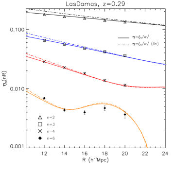
Figure 1: Left panel: The redshift-space galaxy clustering ratio $\eta_{g,R}(nR)$ (LHS of eq. 21) extracted from 160 independent LasDamas simulations of the distribution of luminous red galaxies (LRG) (see §4). The observable $\eta_{g,R}(nR)$ is shown as a function of the smoothing radius $R$ for four different values of $n$ as indicated in the inset. Simulated observations are compared to the predicted amplitudes of the real-space mass clustering ratio $\eta_{R}(nR)$ (RHS of eq. (21)) for the same values of $n$. Dot-dashed lines show predictions obtained using a linear power spectrum, while solid lines are derived using the non-linear (halofit) model of Smith et al. (2003). Both the galaxy and mass clustering ratios are derived by adopting the same cosmological parameters of the LasDamas simulations. Error bars represent the uncertainties expected from a redshift survey covering a volume 160 times larger than that explored by the LRG sample used in this study.

2.1 Estimating the galaxy clustering ratio

The variance $\sigma^{2}_{g,R}$ and the correlation function $\xi_{g,R}$ of a smoothed density field of galaxies can be estimated from the three-dimensional distribution of galaxies following the procedure outlined in Bel & Marinoni (2012). We assume that the random variable $N$ models the number of galaxies within typical spherical cells (of constant comoving radius $R$) and consider the dimensionless galaxy excess

$$\delta_{N}\equiv\frac{N}{\bar{N}}-1,$$ (6)

where $\bar{N}$ is the mean number of galaxies contained in the cells.

To estimate the one-point second-order moment of the galaxy overdensity field ($\kappa_{2}=\langle\delta_{N}^{2}\rangle_{c}$), we fill the survey volume with the maximum number ($n_{t}$) of non-overlapping spheres of radius $R$ (whose centre is called a seed) and we compute

$$\hat{\kappa}_{2}=\frac{1}{n_{t}}\sum_{i=1}^{n_{t}}\delta_{N,i}^{2},$$ (7)

where $\delta_{N,i}$ is the dimensionless counts excess in the $i$-th sphere.

The two-point second-order moment $\kappa_{11}=\langle\delta_{Ni}\delta_{Nj}\rangle_{c}$ follows from a generalization of this cell-counting process. To this purpose, we add a motif of isotropically distributed spheres around each seed and retain as proper seeds only those for which the spheres of the motifs lie completely within the survey boundaries. The centre of each new sphere is separated from the proper seed by the length $r=nR$ (where $n$ is a generic real parameter usually taken to be an integer without loss of generality), and the pattern is designed in such a way as to maximize the number of quasi non-overlapping spheres at the given distance $r$. In this study, as in Bel and Marinoni (2012), the maximum allowed overlap between contiguous spheres is set to $2\%$ in volume. This value represents a good comprise between the need to maximize the number of the spheres that are correlated to a given seed and the volume probed by them. If there is a substantial overlap of the spheres of the motif, all the signal on the correlation scales r is fully sampled. However, this strategy is computationally expensive. On the other hand, if the number of spheres is too small, then a substantial fraction of the information available at a given correlation scale $r$ is lost. We have verified that varying this threshold in the range $2$%- $50$% does not modify the estimation of one- and two-point statistical properties of the counts.

An estimator of the average excess counts in the $i$ and $j$ cells at separation $r$ is

Figure 2: The redshift-space galaxy clustering ratio $\eta_{g,R}(nR)$ extracted from the LasDamas simulations (see §4) using $R=14h^{-1}$Mpc and $n=3$ is shown as a function of redshift. Markers represent the average measurement from 40 LasDamas mock catalogues, each of them simulating a redshift survey that has the same radial density profile and observational selection effects as the LRG sample of SDSS DR7. Simulated observations are compared to the predicted amplitudes of the real-space mass clustering ratio $\eta_{R}(nR)$ (right-hand side of eq. (21). Dashed lines show predictions computed using a linear power spectrum, while solid lines are derived assuming the non-linear (halofit) model of Smith et al. (2003). Both the galaxy and mass clustering ratios are estimated by adopting the same cosmological parameters as the LasDamas simulations. Error bars represent the uncertainty from measurements in a single mock catalogue. They are obtained as the standard deviation of 40 independent measurements, therefore including the contribution due to cosmic variance.

$$\hat{\kappa}_{11}=\frac{1}{n_{t}n_{mot}}\left\{\sum_{i=1}^{n_{t}}\delta_{N,i}\sum_{j=1}^{n_{mot}}\delta_{N,ij}\right\},$$ (8)

where $n_{mot}$ is the number of spheres in the motif, and where $\delta_{N,ji}$ is the excess count in the motif’s cell $j$ at distance $r$ from the seed $i$.

It is natural, or at least convenient, to model the spatial point distribution of galaxies as a process resulting from the discrete sampling of an underlying continuous stochastic field $\lambda_{g}({\bf x})$. The quantity of effective physical interest to which we want to have access is thus $\delta_{g,R}({\bf x})\equiv\Lambda_{g}({\bf x})/{\bar{\Lambda}_{g}}-1$, where $\Lambda_{g}({\bf x})=\int_{V({\bf x})}\lambda({\bf x^{\prime}})d{\bf x^{\prime}}$ is the continuous limit of the discrete counts $N$ in volume V. As a consequence, it is necessary to correct counting estimators for discreteness effects. To this purpose and following standard practice in the field, we model the sampling as a local Poisson process (LPP, Layser (1956)). Specifically, we map moments of the discrete variable N into moments of its continuous limit by using

$$\langle\Lambda_{g}^{k}\rangle=\langle N(N-1)...(N-k+1)\rangle\equiv\langle(N)_{f}^{k}\rangle,$$ (9)

in the case of one-point statistics, and its generalization (Szapudi & Szalay 1997; Bel & Marinoni 2012)

$$\langle\Lambda_{g}^{k}({\bf x}_{1})\Lambda_{g}^{q}({\bf x}_{2})\rangle=\langle(N_{1})_{f}^{k}(N_{2})_{f}^{q}\rangle,$$ (10)

for the two-point case. As a result, the estimators of the variance and the correlation function, corrected for shot noise effects, are (Szapudi, Szalay & Boschán 1992; Bel & Marinoni 2012)

$$\hat{\sigma}_{g,R}^{2} = \hat{\kappa}_{2}-\bar{N}^{-1}$$

$$\hat{\xi}_{g,R} = \hat{\kappa}_{11}.$$ (11)

By construction, the $\eta$ observable is not sensitive to the shape of the radial selection function, if the density gradient is nearly constant on scales $r\sim 2R$. Sample-dependent corrections are mandatory, instead, if the survey geometry is not regular; i.e., a significant fraction of the counting cells overlap the survey boundaries. Bel et al. (2013), for example, show how to minimize the impact of radial (redshift) and angular incompleteness when the $\eta$ estimator is applied to a survey, the VIMOS Public Extragalactic Redshift Survey (VIPERS, Guzzo et al. 2013), characterized by non-trivial selection functions.

The scaling of the galaxy clustering ratio $\eta_{g,R}(nR)$ as a function of both $R$ and $n$ is shown in figure 1. That galaxies tend to cluster on small cosmic scales is revealed by the fact that the amplitude of $\eta$ decreases monotonically as a function of the correlation scale $r$. In other terms, the probability of finding two cells with density contrasts of equal sign is suppressed as the separation between the cells increases. The trend of $\eta_{g,R}(r)$ as a function of $R$ (for a given fixed value of $r$) is the opposite, implying that the relative loss of power that results from filtering the field on larger and larger scales is stronger in one-point than in two-point statistics (at least when second-order moments are considered.) We also note that, for constant values of $n$, $\eta_{g,R}(nR)$ decreases monotonically as a function of the smoothing radius $R$ only if the field is correlated on small scales, i.e. $n<4$. For higher $n$ values, in fact, the clustering ratio becomes sensitive to the baryon acoustic oscillations (BAO) imprinted on the large scale distribution of galaxies. As a consequence, a peak shows up at $n=l/R$, where $l$ is the position of the BAO relative maximum in the correlation function of galaxies.

3 Theoretical predictions for the amplitude of the clustering ratio

It is straightforward to predict the theoretical value of the second-order galaxy clustering ratio $\eta_{g,R}$. On large enough cosmic scales $R$, matter fluctuations are small and are described by the linear power spectrum

$$\Delta^{2}(k,{\bf p})=4\pi Ak^{n_{s}+3}T^{2}(k,{\bf p}),$$ (12)

where $A$ is a normalization factor, $n_{s}$ the primordial spectral index, and $T^{2}$ the transfer function. (In this study we assume the analytic approximation of Eisenstein & Hu 1998.) Accordingly, the amplitudes of the second-order statistics for mass evolve as a function of redshift ($z$) and scale ($R$) as

$$\sigma^{2}_{R}(z,{\bf p})=\sigma^{2}_{8}(z=0)D^{2}(z){\mathcal{F}}_{R}({\bf p}),$$ (13)

and

$$\xi_{R}(r,z,{\bf p})=\sigma_{8}^{2}(z=0)D^{2}(z){\mathcal{G}}_{R}(r,{\bf p}).$$ (14)

Both these equations are normalized on the scale $r_{8}=8h^{-1}$Mpc, where $D(z)$ represents the linear growing mode (Weinberg 2008), while the effects of filtering are incorporated in the functions

$${\mathcal{F}}_{R}({\bf p})=\frac{\int_{0}^{+\infty}\Delta^{2}(k,{\bf p})\hat{W}^{2}(kR)d{\rm ln}k}{\int_{0}^{+\infty}\Delta^{2}(k,{\bf p})\hat{W}^{2}(kr_{8})d{\rm ln}k}$$ (15)

$${\mathcal{G}}_{R}(r,{\bf p})=\frac{\int_{0}^{+\infty}\Delta^{2}(k,{\bf p})\hat{W}^{2}(kR)j_{0}(kr)d{\rm ln}k}{\int_{0}^{+\infty}\Delta^{2}(k,{\bf p})\hat{W}^{2}(kr_{8})d{\rm ln}k}$$ (16)

where $j_{n}(x)$ is the spherical Bessel function of order $n$, and $\hat{W}$ is the Fourier transform of the window function. In this analysis we adopt a spherical top hat filter for which

$$\hat{W}(kR)=\frac{3}{kR}j_{1}(kR).$$ (17)

By analogy with the galaxy clustering ratio, we can now define the mass clustering ratio as

$$\eta_{R}(r,{\bf p})=\frac{{\mathcal{G}}_{R}(r,{\bf p})}{{\mathcal{F}}_{R}({\bf p})}.$$ (18)

The relationship between the mass and galaxy clustering ratios in real space follows immediately once we specify how well the overall matter distribution is traced by its luminous subcomponent on a given scale $R$. On large enough scales, such as those explored in this paper, a local, deterministic, non-linear biasing scheme (Fry & Gaztañaga 1993), namely

$$\delta_{g,R}({\bf x})=\sum_{i=0}^{N}(b_{i,R}/i!)\delta_{R}^{i}({\bf x}),$$ (19)

offers a fair description of the mapping between mass and galaxy density fields. The scale-dependent parameters $b_{i,R}$ are called biasing parameters, and within the limits $\sigma_{R}^{2}<<|b_{1,R}/b_{2,R}|$ and $\xi_{R}<<1/b_{2}$ (see eq. 28 of Bel & Marinoni 2012), one has

$$\sigma^{2}_{g,R}({\bf r}) \approx b_{1,R}^{2}\sigma^{2}_{R}({\bf r})$$

$$\xi_{g,R}({\bf r}) \approx b_{1,R}^{2}\xi_{R}({\bf r}).$$ (20)

We therefore deduce that

$$\eta_{g,R}(r,{\bf p})=\eta_{R}(r,{\bf p}),$$ (21)

a relation independent of the specific value of the bias amplitudes $b_{1R}$.

The conditions under which eq. (21) is derived are quite generic and are fulfilled once the field is filtered on sufficiently large scales $R$ and/or once the second-order bias coefficient is negligible compared to the linear bias term. This last requirement is satisfied for large $R$ (for example, Marinoni et al. (2005, 2008b), using VVDS galaxies at $z=1$ (Le Fèvre et al. 2005), find $|b_{2,R}/b_{1,R}|\sim 0.17\pm 0.07$ for $R=10h^{-1}$Mpc, a result implying that, at least on these scales, any eventual scale dependence of the biasing relation is also negligible.

Figure 3: Left: Isocontours of the function $\eta_{g,R}/\eta_{g,R}^{bestfit}-1$ displaying the relative variation in the galaxy clustering ratio (with respect to the best-fitting value deduced from the analysis of SDSS DR7 data) induced by a wrong choice of the distance-redshift conversion model (i.e. a wrong guess of the cosmological parameters $[\Omega_{m},\Omega_{X}]$). The galaxy clustering ratio is reconstructed on the scales $(R,r)=(14,42)h^{-1}$Mpc, and its expression is approximated well by eq. (25). The best-fitting cosmology inferred from the analysis of SDSS DR7 data is $\Omega_{m}=0.28,\Omega_{X}=0.45,w=-1.2$. The isocontours measure the strength of the AP geometric distortions. Right: the relative variation in the mass clustering ratio $\eta_{R}/\eta_{R}^{bestfit}-1$ that results from computing the power spectrum in the wrong cosmology.

The most interesting aspect of eq. (18) is that, in the linear limit, it is effectively insensitive to redshift distortions, and, therefore, independent of their specific modelling. In other terms, the ratio $\eta_{R}(r,{\bf p})$ between second-order statistics has identical amplitude in both real- and redshift-space. If the only net effect of peculiar velocities is to enhance the amplitudes of the density ripples in Fourier space, without any change in their phases or frequencies (as predicted, for example, by the Kaiser model, Kaiser 1987), then redshift distortions contribute equally to the numerator and denominator of eq. (18). This simplifies the interpretation of the master equation (21): its left-hand side (LHS) can be estimated using galaxies in redshift space, while its right-hand side (RHS) can be theoretically evaluated in real space. This factorization property holds because the $\eta$ statistic is only sensitive to the monopol of the power spectrum, i.e. to the quantity obtained by averaging the redshift-space anisotropic power spectrum $P_{z}({\bf k})$ over angles in k space ($\int_{-1}^{1}P^{z}(k,\mu_{k})d\mu_{k}$, where $\mu_{k}$ is the cosine of the angle between the $k$ vector and the line-of-sight). Indeed, as explained in section 2.1, to estimate $\eta$, we position an isotropic distribution of cells (the motif) around each seed.

Another salient property is that, as long as a linear matter’s power spectrum is assumed, the mass clustering ratio $\eta_{R}$ is effectively independent of the amplitude of the matter power spectrum normalization parameter $A$. In linear regime, i.e. when $R$ is sufficiently large, the clustering ratio is also independent of redshift. This property is graphically illustrated in Fig. 2. This comes about because the only time dependence appearing in the expression of the variance and correlation function of a smooth density field is through the growing mode $D(z)$, a quantity that, on large linear scales, appears in the relevant equations as a multiplicative parameter that eventually factors out in the $\eta$ ratio. Figure 2 shows that, on large scales and sufficiently low redshift, this property still holds even when a non-linear description of the matter power spectrum is adopted. Specifically, it shows that the mass clustering ratio predicted using the non-linear power spectrum of Smith et al. (2003) is effectively time independent. In conclusion, for any given filtering ($R$) and correlation ($r$) scales, the mass clustering ratio $\eta_{R}(r,{\bf p})$ behaves as a cosmic ‘standard of clustering’, a quantity that does not evolve across cosmic time.

The bias free property of eq. (21) also deserves further comment. Since the smoothing and correlation are performed on fixed scales $R$ and $r$, $\eta_{g,R}$ is not a function but a number. Although one can estimate it using any given visible tracer of the large scale structure of the universe, this number captures second-order information about the clustering of the general distribution of mass. This conclusions holds as long as eq. 19 provides a fair description of the nature of biasing on large scales $R$, which is as long as the matter - galaxy relation is deterministic and local. In this regard we remark that the galaxy density is likely to show some scatter around the dark matter density due to various physical effects. This stochasticity, however, is not expected to influence the accuracy of the equation (21) in a significant way. On large scales, the only effect stochasticity might introduce is a rescaling of the linear biasing parameter by a constant (Scherrer & Weinberg 1998). Because it is defined as a ratio, $\eta$ is unaffected by such a systematic effect. A second source of concern comes from the fact that the $\eta$ formalism is built out of the hypothesis that biasing is local; i.e., we can neglect the possible existence of scale dependent operators in the matter-galaxy density relations, at least on large smoothing scales $R$. A simple argument provides the guess for the sensitivity of the clustering ratio to this assumption. In the limit in which $r>R$, $\hat{W}^{2}(kR)j_{0}(kr)\sim j_{0}(kr)$, the mass clustering ratio scales approximatively as

$$\eta_{R}(nR,{\bf p})\propto\frac{\Delta^{2}(k_{j_{0}},\bf{p})}{\Delta^{2}(k_{W_{0}},{\bf p})},$$ (22)

where, quite crudely, $k_{j_{0}}$ and $k_{W_{0}}$ can be estimated as the wave vectors where the amplitude of the low pass filters $j_{0}(kr)$ and $\hat{W}^{2}(kR)$ falls to one half. The proposed test, therefore, exploits neither the absolute amplitude nor the full shape of the power spectrum, but only its relative strength on two distinct $k$ scales. By choosing to correlate the field on scales $r$ that are not too large compared to the smoothing scale $R$, it is possible to minimize the impact of any eventual $k-$dependent bias.

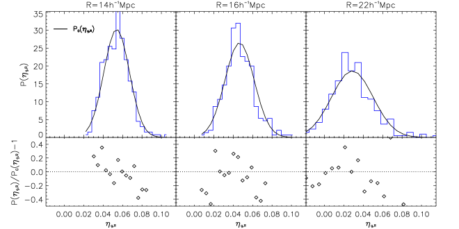
Figure 4: Upper panels: the distribution of the galaxy clustering ratio $\eta_{g,R}(r)$ obtained by analysing 160 LasDamas mock catalogues simulating the distribution of luminous red galaxies (histograms). The observable $\eta_{g,R}(r)$ is computed for the three different smoothing radii $R$ shown on top of each plot and by assuming, furthermore, that $r=3R$. The solid line displays the best-fitting Gaussian PDF. Lower panels: the relative deviation between the Gaussian model and the actual distribution of the data is shown.

3.1 Precision and accuracy of the $\eta$ formalism

The next step is to make sure that systematic effects, whether physical (such as any eventual non-locality in the biasing relation), observational (like systematic errors in estimating the relevant observables from data), or statistical (that, for example, although the estimator in eq. (5) is a ratio of unbiased estimators, it does not necessarily to be unbiased itself) do not compromise the effectiveness of the formalism in practical applications. We therefore use numerical simulations of the large scale structure to compare the amplitude of the redshift space galaxy clustering ratio (the LHS of eq. (21)) and the theoretically predicted value of the real space mass clustering ratio (the RHS of eq. (21)). Figure 1 shows that, on scales $R>10h^{-1}$Mpc and $r=3R$, equation (21) is good to better than $1\%$, and to better than $0.1\%$ on scales larger than 15$h^{-1}$Mpc (for the same correlation length $r=3R$). This last figure is two orders of magnitude smaller than the precision achievable when measuring $\eta_{g,R}(r)$ using current data ($\sim 7\%$ see Sec IV). Simulations also indicate that, for smoothing scales $R<15h^{-1}$Mpc, the precision achieved by using a non-linear power spectrum (in our case the phenomenological prescription of Smith et al. 2003) is nearly a factor of five better than the one obtained by adopting a simple linear model.

It is impressive how this remarkable sub-percentage precision in mapping theory onto real-world observations is achieved without introducing any external non-cosmological information, such as any explicit biasing parameter or any model that corrects galaxy positions for non-cosmological redshift distortions. Nonetheless, for very large separations (i.e. $r=6R$), theoretical predictions fail to reproduce observations. As a matter of fact, when the field is smoothed on a scale $R=16h^{-1}$Mpc and correlated on a scale $r=16\times 6\sim 100h^{-1}$Mpc, the $\eta$ indicator becomes extremely sensitive to the specific features of the baryon acoustic oscillations imprinted in the galaxy distributions. Indeed, from a theoretical point of view, the correlation function of the smoothed density field results from convolving the correlation function of galaxies over two smoothing windows of radius $R$ at positions ${\bf x}_{1}$ and ${\bf x}_{2}$ separated by the distance ${\bf r}$

$$\xi_{R}({\bf r})=\frac{1}{V_{R}^{2}}\int_{V_{R({\bf x}_{1})}}d{\bf y}_{1}\int_{V_{R({\bf x}_{2})}}d{\bf y}_{1}\xi({\bf y}_{1},{\bf y}_{2}).$$ (23)

This convolution preserves the position of the BAO peak, but it decreases its amplitude and broadens its width. Notwithstanding, it is still possible to detect the BAO scale in a precise way using the eta estimator. As the poor agreement between theory and measurements of Fig. 1 shows, however, the simple power spectrum models described above are not able to grasp the non-linear physics involved in this phenomenon. The modelling of local peculiar motions is also paramount if we are to predict the BAO profile to the precision required for cosmological purposes.

At the opposite limit, when the field is correlated on small scales $(r=2R)$, the mass clustering ratio fits observations in a better way if the non-linear prescription of Smith et al. (2003) is considered instead of the linear power spectrum. In other terms, numerical simulations indicate that once the $\delta-$field is coarse grained on a sufficiently large scale $R$, a linear power spectrum captures the essential physics governing the clustering of galaxies only if the field is correlated on scales $3\leq n<6$.

3.2 The clustering ratio as a cosmic probe

Apart from the most immediate use as a statistic to measure the clustering of mass in a universal (sample-independent) way, the clustering ratio can also serve as a tool to set limits to the value of cosmological parameters. The RHS of eq. (21) relies upon the theory of cosmological perturbations, and it is fully specified (it is essentially analytic) given the shape of the mass power spectrum in real space. Therefore it is directly sensitive to the shape ($n_{s}$) of the primordial power spectrum of density fluctuations, as well as to the parameters determining the shape of the transfer function of matter perturbations at matter-radiation equality (in particular, the present-day extrapolated value of the matter ($\Omega_{m}h^{2}$) and baryon ($\Omega_{b}h^{2}$) density parameters. The possible contribution of massive neutrinos is neglected in this analysis.) By contrast, the LHS term of eq. (21) probes the structure of the comoving distance-redshift relation, therefore it is fully specified once the homogeneous expansion rate history of the universe is known. On top of $\Omega_{m}$, the LHS term is thus also sensitive to $\Omega_{X}$ and $w$, i.e. to a wide range of DE models. If distances are expressed in units of $h=H_{0}/100$ km s^-1Mpc^-1, the LHS is effectively independent of the value of the Hubble constant $H_{0}$.

The possibility of constraining the true cosmological model follows from noting that the equivalence expressed by eq. (21) holds true if and only if the LHS and RHS are both estimated in the correct cosmology. Analytically, the amplitudes of the galaxy clustering ratio $\eta_{g,R}(r)$ and of the mass clustering ratio $\eta_{R}(r)$ do not match if clustering is analysed by assuming the wrong cosmology; since the derivatives with respect to the parameters ${\bf p}$ of the LHS and RHS of eq. 21 are not identical. Physically, two effects contribute to breaking the equivalence expressed by eq. 21 when a wrong set of parameters ${\bf p}$ is assumed: geometrical distortions, the Alcock and Paczynski (AP) signal (Alcock & Paczynski 1979; Ballinger, Peacock & Heavens 1996; Marinoni & Buzzi 2010), dynamical effects, and distortions in the power spectrum shape. By AP, we mean the artificial anisotropy in the clustering signal that results when the density field is correlated using the wrong distance-redshift relation. In this case, and contrary to what one would expect on the grounds of symmetry considerations, the clustering power in the directions parallel and perpendicular to the observer’s line of sight is not statistically identical. Transfer function shape distortions, the second source of sensitivity to cosmology, are generated by evolving the relevant mass statistics in the wrong cosmological background, and they can be traced primarily to the spurious modification of the size of the horizon scale at the epoch of equivalence.

The amplitude of AP and power spectrum distortions are compared in Fig. 3. Geometric effects (for $R=14h^{-1}$Mpc and $r=3R$), are almost completely degenerate with respect to the $\Omega_{m}$ parameter, that is for any given fixed value of $\Omega_{X}$, the amplitude of the AP signal is nearly independent of $\Omega_{m}$. On the contrary, the distortions in the observable $\eta_{g,R}$ induced by a wrong guess of the dark energy parameter are an increasing function of $\Omega_{X}$: the amplitude of the clustering ratio is underestimated(/overestimated) by at most $20\%$ when $\Omega_{X}$ varies in the interval $[0,1]$. Power spectrum distortions, instead, which are by definition independent of $\Omega_{X}$, are extremely sensitive to the matter density parameter $\Omega_{m}$. A change of $\sim\pm 0.1$ of the true value (in this case $\Omega_{m}=0.28$) results in a change of $\eta_{R}$ by nearly $\pm 50\%$. We conclude that, given the uncertainty characterizing the SDSS data analysed in this paper, the AP signal is marginal – but it will become an interesting constraint on dark energy with larger datasets, such as Euclid (Laureijs et al. 2011).

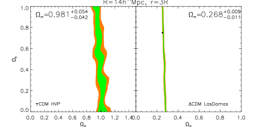
Figure 5: Left panel: two-dimensional confidence limits on $\Omega_{m}$ and $\Omega_{\Lambda}$ from a ‘blind’ analysis of the $\tau$CDM HVP simulation (Jenkins et al. 2001). Contours are plotted for ${\mathcal{L}}/{\mathcal{L}}_{min}<2.3,6.17$ corresponding to $68$ and $95$ per cent c.l. for a multivariate Gaussian distribution with 2 degrees of freedom. The relevant one-dimensional marginalized constraint is shown in the legend. The clustering ratio $\eta_{g,R}(r,{\bf p})$ is estimated using $R=14h^{-1}{\mathrm{M}pc}$ and $r=3R$. For the best-fitting cosmology we measure $\eta_{g,R}(r,{\bf p}^{f})=0.0294\pm 0.0017$ where the error is evaluated via $30$ jackknife resampling of the data, excluding each time a sky area of $36\times 19.5$ deg². Dirac delta priors are taken of $\Omega_{b}h^{2}$, $H_{0}$, and $n_{s}$, that are centred on the simulated values. Right panel: same as before, but now contours represent the joint likelihood analysis of $40$ independent $\Lambda$CDM mock catalogues simulating the SDSS LRG sample. For the best-fitting cosmology we find $\eta_{g,R}(r,{\bf p}^{f})=0.0573\pm 0.0008$, where the error, computed as the s.d. of the mean of $40$ measurements, includes the contribution from cosmic variance.

Figure 6: Upper: the variance $\sigma_{g,R}=\xi_{g,R}(0)$ of the SDSS LRG sample as a function of the filtering scale $R$ for 2 different sets: the full sample (diamonds) and the subsample containing the brightest $50\%$ (in the $r$ band). Centre: the correlation function $\xi_{g,R}(3R)$ of the smoothed galaxy density field is shown as a function of $R$ for the same subsets. Both the variance and the correlation function are estimated in the best-fitting cosmological model. Lower: the amplitude of the galaxy clustering ratio $\eta_{g,R}(3R)$ is demonstrated to be the same for these two samples of biased tracers of the large scale distribution of matter. Also shown is the theoretically predicted scaling of the mass clustering ratio (dot-dashed line). This last quantity is computed assuming the best-fitting cosmological parameters ${\bf p}^{f}=(0.28,0.45,-1.2,73.8,0.0213,0.96)$ deduced from analysis of the whole LRG sample on the specific scale $R=14h^{-1}$Mpc. In all the panels, error bars are derived from 30 block-jackknife resampling of the data, excluding, each time, a sky area of $12\times 14$ deg².

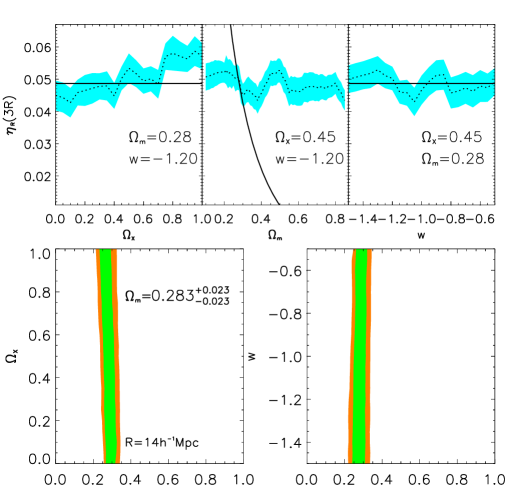
Figure 7: Upper panels: The galaxy clustering ratio $\eta_{g,R}(r,\Omega_{m},\Omega_{X},w)$ (dotted line) reconstructed from SDSS DR7 data assuming $R=14h^{-1}$Mpc and $r=3R$, plotted as a function of $\Omega_{\Lambda}$ (left), $\Omega_{m}$ (centre) and $w$ (right), after fixing the remaining cosmological parameters, shown in the inset, to the values that minimize the logarithmic posterior (24). Grey shading is the $1-$sigma deviation around the mean, and it is computed from 30 block-jackknife resampling of the data. This uncertainty depends on cosmology (because of the redshift-distance conversion model) in a stochastic way ($\pm 20\%$ around the mean, for the cosmologies shown in the picture). We also show the predicted scaling of the mass clustering ratio (solid line) in the corresponding cosmology. The best set of cosmological parameters ${\bf p}^{f}=(0.28,0.45,-1.2,73.8,0.0213,0.96)$ is the very one that minimizes the difference between theoretical predictions (line) and actual data (points). For SDSS DR7 data, we find $\eta_{g,R}(3R,{\bf p}^{f})=0.0502\pm 0.0036$ on a scale $R=14h^{-1}$Mpc. Lower panels: two-dimensional marginalized constraints on a curved XCDM model in which both $\Omega_{X}$ and $w$ are allowed to vary. Gaussian priors are taken of $\Omega_{b}h^{2}=0.0213\pm 0.0010$, of $H_{0}=73.8\pm 2.4$ km s^-1Mpc^-1 and of $n_{s}=0.96\pm 0.014$ from BBN (Pettini et al. 2008), HST (Riess et al. 2011) and WMAP7 (Larson et al. 2011) determinations, respectively. Contours are plotted for ${\mathcal{L}}/{\mathcal{L}}_{min}<2.3,6.17$.

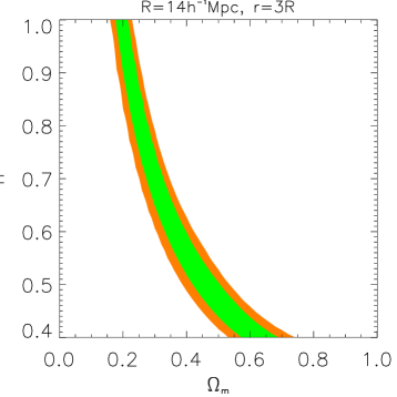
Figure 8: Two-dimensional marginalized constraints on $\Omega_{m}$ and $H_{0}$ obtained by fitting data with a curved XCDM model. Contours are plotted for ${\mathcal{L}}/{\mathcal{L}}_{min}<2.3,6.17$ Gaussian priors are taken of $\Omega_{b}h^{2}=0.0213\pm 0.0010$ and $n_{s}=0.96\pm 0.014$ from BBN (Pettini et al. 2008) and WMAP7 (Larson et al. 2011) determinations, respectively.

We now illustrate how, in practice, we evaluate $P({\bf p}|\eta_{g,R})$, the likelihood of the unknown set of parameters ${\bf p}=(\Omega_{m},\Omega_{X},w,H_{0},\Omega_{b}h^{2},n_{s})$ given the actual value of the observable $\eta_{g,R}$. The analysis does not require any specification of further model parameters other than those quoted above.

The probability distribution function of the clustering ratio is not immediately obvious since this observable is defined via a ratio of two non-independent random variables. Simulated and real data suggest that it is fairly accurate to assume that the PDF of $\eta_{g,R}$ is approximately Gaussian. This is demonstrated in Fig. 4. As a result, the most likely set of cosmological parameters (${\bf p}^{f}$) is the one that minimizes the logarithmic posterior ${\mathcal{L}}=-\log P$

$${\mathcal{L}}=\sum^{N}\log\sigma_{\eta,i}+\frac{\chi^{2}}{2}-\log\pi+B,$$ (24)

where $\chi^{2}=\sum^{N}\sigma_{\eta,i}^{-2}(\eta_{g,R}-\eta_{R})^{2}$, where $N$ is the number of estimates of $\eta_{g,R}$, $\sigma_{\eta,i}$ is the error on the observable, $\pi$ describes any a-priori information about the PDF of ${\bf p}$, and where $B$ is a normalization constant that can be fixed by requiring $\int Pd{\bf p}=1$.

Since eq. (21) is free of look-back time effects, the analysis does not require slicing the sample in arbitrary redshift bins. Only one estimation ($N=1$) of eq. (5) is needed across the whole sample volume. We have recalculated the observable $\eta_{g,R}(r,{\bf p})$ for each comoving distance-redshift model, i.e. on a grid $(\Omega_{m},\Omega_{X},w)$ of spacing $[10^{-2},5\cdot 10^{-2},5\cdot 10^{-2}]$. As a consequence, the posterior ${\mathcal{L}}$ does not vary smoothly between different models because the number of galaxies counted in any given cell varies from model to model. However, since computing the observable $\eta_{g,R}(3R,{\bf p})$ takes a limited amount of time, shot noise is the price we have decided to pay to obtain an unbiased likelihood hyper-surface.

4 Blind analysis of cosmological simulations

We assess the performances of the $\eta$ test under realistic operating conditions via a ‘blind’ analysis of mock catalogues that are characterized by widely different sets of expansion rate parameters, power spectrum shapes, mass tracers, and radial selection functions. These are the $\tau$CDM Hubble Volume Project (HVP) simulation (Jenkins et al. 2001) and the $\Lambda$CDM LasDamas simulation (McBride et al. 2009).

The HVP is a synthetic catalogue of clusters of galaxies that covers one octant of sky, extends over the redshift interval $0.1<z<0.43$, is comprised of $\sim 10^{6}$ massive haloes with an average space density of $6\times 10^{-4}h^{3}{\mathrm{M}pc}^{-3}$, and it was simulated using ${\bf p}^{i}=(1,\;0,\;-1,\;21,\;0,\;1)$. An end-to-end analysis of clusters mock data (HVP) allows us to check for any insidious algorithmic biases that could arise when training a method to ‘recognize’ only a fiducial $\Lambda$CDM cosmology via a single class of biased tracer of the matter clustering pattern, namely galaxies. The left-hand panel of Fig. 5 shows that the input value $\Omega_{M}=1$ is statistically retrieved.

The $\Lambda$CDM LasDamas simulations are a set of 40 nearly independent galaxy simulations that cover $120\times 45$ deg², extend over the redshift interval $0.16<z<0.43$, are comprised of $\sim 60000$ galaxies each, and have an average space density of $\sim 8.9\times 10^{-5}h^{3}{\mathrm{M}pc}^{-3}$. The mock catalogues are obtained from N-body simulations (whose input cosmological parameters are ${\bf p}^{i}=(0.25,\;0.75,\;-1,\;70,\;0.0196,\;1)$) by populating dark matter haloes with galaxies according to a halo occupation distribution function. The structural parameters of this statistic, which describes the probability distribution of the number of galaxies in a halo as a function of the host halo mass, are fixed using SDSS data. These catalogues, which incorporate all the observing selections of the SDSS luminous red galaxies survey, i.e. the real data sample used in our analysis (see §5), allow us to verify that the specific SDSS observing biases do not spoil our cosmological inferences. Another advantage is that we can forecast the statistical (and systematic) fluctuations in the observable and compare this figure, which includes contribution from cosmic variance, with the uncertainty in $\eta$ directly estimated from SDSS DR7 data via a block-jackknife technique (see §5).

The encouraging outcome of the analysis of these SDSS like data is presented in Fig. 5, where we show the cosmological bounds that could be obtained from a redshift survey having a volume 40 times larger than is probed by the SDSS DR7 LRG sample ($\sim 1/2$ of the volume that will be measured by surveys such as EUCLID (Laureijs et al. 2011) or BigBOSS (Schlegel et al. 2011)). This figure shows that one can constrain $\Omega_{m}$ precisely ($\sim 3.7\%$) and accurately (the input value is recovered within the $95\%$ c.l.). Whereas a proper analysis of an EUCLID-like simulation is beyond the purposes of the present work, our clustering analysis in a comparable volume is already suggestive of the robustness with which future data will allow constraining the matter density parameter. As Fig. 2 indicates, pushing the technique to its limit, at least on a scale $R=14h^{-1}Mpc$, only requires incorporating predictions from a non-linear matter power spectrum. Finally, the strong sensitivity to the abundance of matter of the clustering ratio essentially arises because the zero-order spherical Bessel function in eq. (3) filters different portions of $\Delta^{2}$ when $\Omega_{m}$ is changed. If we bias high $\Omega_{m}$, the suppression of power in $\xi_{R}(r,{\bf p})$ on a scale $r$ is more than what is observed when estimating $\xi_{g,R}(r,{\bf p})$ using the corresponding wrong distance-redshift relation (see Fig. 3).

5 Cosmological constraints from the SDSS DR7 sample

We now present and discuss cosmological constraints inferred from the analysis of the LRG sample extracted from the SDSS DR7.

The geometry of the subsample that we have analysed is dictated by the need of sampling the galaxy distribution with cells of radius $R$, as well as of correlating cell counts on scales $r$. The inferior limit on $R$ is set as to simplify our analysis. Although not mandatory, by framing the analysis in the linear domain, i.e. by choosing an inferior threshold for $R$, we avoid introducing any phenomenological description of the matter power spectrum. It is true that this choice prevents us from extracting the maximum information from the data; however, it makes the data analysis more transparent. For example, by adopting as a model the quasi linear model (halofit) of Smith et al. (2003) for the non-linear power spectrum, we would be forced to add an extra component, $\sigma_{8}(0),$ to the vector of unknown parameters ${\bf p}$, therefore complicating unnecessarily the likelihood analysis and the marginalization procedures. The choice of $R$ is additionally conditioned by the practical requirement of minimizing the shot noise contribution in each cell, i.e. $R>(4\pi\rho/3)^{-1/3}$. In this work we adopt the scale $R=14h^{-1}$Mpc. The lower limit $r=3R$ on the correlation scale, instead, is set to guarantee optimal accuracy in the approximation (21). At the opposite end, the higher the values of $R$ and $r$, the less the inferred cosmological predictions are informative. The sample that complies with these constraints covers the redshift interval $0.15<z<0.43$, has a contiguous sky area of $120\times 45$ deg², and is comprised of $62,652$ LRG (corresponding to 55% of the total number of LRG contained in DR7), with a mean density of $9.2\times 10^{-5}h^{3}{\mathrm{M}pc}^{-3}$.

The $R-$scaling of the variance $\sigma_{g,R}$ and correlation function $\xi_{g,R}(nR)$ of the smoothed galaxy density field is shown in Fig. 6. The amplitude of both these observables is not a universal quantity. In addition to the background cosmological model, it also depends on the particular set of luminous objects used to trace the mass density field. That bright galaxies display stronger $rms$ fluctuations and are more strongly correlated than faint ones as shown in Fig. 6. This same figure also shows that the amplitude of $\xi_{g,R}$ is nearly one order of magnitude smaller than $(\sigma_{g,R})$. The lack of power in the two-point statistic is theoretically expected, since only in the limit for $r\rightarrow 0$ does the correlation function of a smoothed field converge to the variance, i.e. $\xi_{g,R}(0)=\sigma^{2}_{g,R}$. Given that in a sample of $N$ cells, the number of independent combinations of two cells is smaller than $N$, we also expect the two-point statistic to be estimated with larger uncertainties than the corresponding one-point statistic of equal order. For example, the SDSS DR7 sample allows us to extract the value of $\xi_{g,R}(/\sigma^{2}_{R})$ with a precision of $6.5\%(/5\%)$ when the field is smoothed on the scale $R=14h^{-1}$Mpc. As far as the functional dependence on $R$ is concerned, the scaling of both these statistics is essentially featureless and approximated well by a power law over the interval $12<R<20h^{-1}$Mpc. For a given fixed value of $n$, the relative loss of power resulting from filtering the field on larger and larger scales $R$ is stronger for $\xi_{g,R}(nR)$ than $\sigma^{2}_{g,R}$.

The galaxy clustering ratio $\eta_{g,R}(nR)$ estimated in the best-fitting cosmology is shown in Fig. 6. This observable is a universal quantity associated to the mass density field, and, as such, it is independent of the specific biasing properties of the mass tracers adopted in this analysis. The precision with which the clustering ratio is determined from SDSS LRG data ($\sigma_{\eta}/\eta\sim 7\%$ on a scale $R=14h^{-1}$Mpc) is estimated from 30 jackknife resampling of the data each time excluding a sky area of $12\times 14$ deg². This figure is in excellent agreement with the one ($\sim 8\%$) deduced from the analysis of the standard deviation displayed by the $40$ SDSS-like simulations LasDamas, which include, by definition, the contribution from cosmic variance. This indicates that $\eta$, which is defined as a ratio of equal order statistics and thus contains the same stochastic source, is weakly sensitive to this systematic effect. We note that the relative uncertainty on $\eta_{g,R}(nR)$ cannot be simply deduced via standard propagation of errors since measurements of $\sigma^{2}_{g,R}$ and $\xi_{g,R}$ are positively correlated.

Without fixing either the curvature of the universe (flat prior $0<|\Omega_{k}|<1$) or the quality of the DE component (flat prior $-3/2<w<-1/2$), but taking (strong) Gaussian priors of $\Omega_{b}h^{2}$, $H_{0}$, and $n_{s}$ from big bang nucleosynthesis (BBN, Pettini et al. (2008)), Hubble Space Telescope (HST, Riess et al. (2011)), and WMAP7 (Larson et al. 2011), respectively, we constrain the local abundance of matter $\Omega_{m}$ with a precision of $8\%$ ($\Omega_{m}=0.283\pm 0.023$, see Fig. 7. For the sake of completeness, by choosing a smoothing scale of $18/22h^{-1}$Mpc, we obtain $\Omega_{m}=0.270^{+0.037}_{-0.027}/0.255\pm 0.038$.) This figure improves the precision of the estimate ($\Omega_{m}=0.259\pm 0039$) by a factor of two obtained by analysing, with the same priors, the BAO of the SDSS DR5 sample (which contains 25% fewer galaxies than DR7)(Eisenstein et al. 2005). It also improves by $\sim 20\%$ the precision of the constraint $\Omega_{m}=0.24^{+0.025}_{-0.024}$ that Percival et al. (2010) obtained by combining BAO results from the DR7 sample with the full likelihood of the WMAP5 data (Dunkley et al. 2009) and a strong HST prior (Riess et al. 2009). The value $\Omega_{m}=0.294\pm 0.017$ (Anderson et al. 2012) obtained by combining the BAO results from the DR9 sample (containing 5 times more LRGs than the DR7 catalogue) with the full likelihood of CMB data (WMAP7, Larson et al. 2011) is nearly $40\%$ more precise than our estimate.

The best-fitting value of $\Omega_{m}$ still remains within the quoted $68\%$ contour level (cl), even when we relax some of the strong priors. With a (weak) flat prior on $n_{s}$ (in the interval $[0.9,1.1]$), we obtain $\Omega_{m}=0.271^{+0.030}_{-0.031}$, while if we go on to weaken the prior on $\Omega_{b}h^{2}$ (flat in the interval $[0,0.03]$), we obtain $\Omega_{m}=0.255\pm 0.040$. Although the best-fitting value of $\Omega_{m}$ is weakly sensitive to changes in $\Omega_{b}h^{2}$ and $n_{s}$, Fig. 8 shows that $\Omega_{m}$ degenerates with $H_{0}$ when the HST prior is removed. If we also relax the strong prior on $H_{0}$ (by assuming a flat prior in the interval $[40,100]$km/s/Mpc), we find $\Omega_{m}=0.22^{+0.14}_{-0.04}$. The stability of the best-fitting central value $\Omega_{m}$ is of even more interest if contrasted to CMB results showing that it is the combination $\Omega_{m}h^{2}$ that is insensitive to the prior on the curvature of the universe. On the contrary, if on top of the chosen priors we also impose as constraints that the universe is flat and that dark energy is effectively described by a cosmological constant (i.e. we fix $w=-1$), we obtain $\Omega_{m}=0.275\pm 0.020$, an estimate that improves the WMAP7 bound by $50\%$ ($0.267\pm 0.029$, Larson et al. (2011)). For comparison, the recent combination of the Planck temperature power spectrum with WMAP polarization gives $\Omega_{m,0}=0.315\pm 0.017$.

By switching from precision to accuracy, it is important to point out that the mass-clustering ratio (cf. Eq. 18) computed using the best parameters ${\bf p}$ inferred on a scale $R=14h^{-1}$Mpc correctly predicts the galaxy clustering ratio observed on various different scales $R$ (see lower panel of Fig. 6). This highlights the overall unbiasedness of our cosmological inference.

The Fisher matrix formalism cannot be reliably applied to reproduce constraints on cosmological parameters that are strongly degenerate. A simple way to make sense and reproduce our results consists of working out an effective measure of the observable $\eta_{g,R}(r,{\bf p})$. The relevant cosmological information contained in the SDSS DR7 data can be effectively retrieved by approximating the galaxy clustering ratio $\eta_{g,R}$ via the fitting formula

$$\eta_{g,R}(3R,{\bf p})\!=\!0.0712\!-\!0.0788x_{p}\!+\!0.0981x^{2}_{p}\!-\!0.0538x^{3}_{p}$$ (25)

where $R=14h^{-1}$Mpc, $x_{p}=1+{\mathrm{f}}_{p}/8.48$, and where

$$\begin{array}[]{rl}{\mathrm{f}}_{p}\!=\!&\!3w\Omega_{X}\!-\!\Omega_{k}\!+0.042\left\{w\Omega_{X}[1\!-\!\frac{9}{2}(1+w)w]\!+\!\frac{\Omega_{k}^{2}-5\Omega_{k}}{2}\right\}\\ &+0.29\left\{w\Omega_{X}(14+3w)-3w\Omega_{X}\Omega_{k}+\frac{\Omega_{k}^{2}}{2}-\frac{11}{3}\Omega_{k}\right\}.\end{array}$$

This phenomenological formula allows a fast computation of the value of the observable $\eta_{g,R}$ in any given cosmological model characterized by $0.1<\Omega_{m}<1$, $0<\Omega_{X}<1$, and $-1.5<w<-0.5$. The left-hand panel of Fig. 3 is obtained by setting $w=-1.2$ and by taking isocontours of the resulting two-dimensional surface in the plane $[\Omega_{m},\Omega_{X}]$. By inserting this formula in the likelihood expression (24), and by further assuming $\sigma_{\eta}=0.004$ independently of the cosmological model, one can reproduce the cosmological constraints shown in Fig. 7.

6 Conclusions

The paper presents and illustrates the use of a new cosmic standard of clustering, the galaxy clustering ratio $\eta_{g,R}(r)$, which is defined as the ratio of the correlation function to the variance of the galaxy overdensity field smoothed on a scale $R$. The key result of the analysis, the one that a-posteriori justifies by itself the introduction of this statistic, is the demonstration that there is no need to model the complex physics underpinning galaxy formation and evolution processes if we are to deduce the amplitude of the corresponding mass statistics ($\eta_{R}(r)$) from the observed value of the galaxy clustering ratio ($\eta_{g,R}(r)$) . Indeed, it is straightforward to show that, on large linear scales, $\eta_{g,R}(r)=\eta_{R}(r)$. In other words, what you see (baryon clustering) is what you get (dark matter clustering).

Interestingly, the magnitude of the mass clustering ratio $\eta_{R}(r)$ on the given fixed scales R and r is a number that is neatly related to the relative amplitude of the the real-space mass power spectrum in two distinct bandwidths. This implies that, instead of being characteristic of a specific galaxy sample, the galaxy clustering ratio estimated for the pair of linear scales R and r is a universal quantity that only depends on the initial distribution of matter density fluctuations and on the nature of dark matter.

Many other cosmological observables probe information encoded in second-order mass statistics. The distinctiveness of the galaxy clustering ratio resides primarily in its simplicity. On large linear scales, its amplitude is independent of galaxy biasing, peculiar velocity modelling, linear growth rate of structures, and normalization of the matter power spectrum. The advantage over standard clustering analyses is both practical and conceptual. The clustering ratio provides a way to extract information about the mass power spectrum without the need to estimate the galaxy power spectrum or the correlation function of galaxies. Moreover, that $\eta_{g,R}(r)$ is estimated via cell-counting techniques on a given fixed pair of scales $(R,r)$ makes the estimation process and the likelihood analysis computationally fast. There is no need, for example, to compute the sample covariance matrix or to speed up calculations by framing the clustering analysis in a given fiducial cosmological model. Additionally, since results do not follow from the reconstruction of the full shape of the galaxy correlation function $\xi(s)$, the cosmological interpretation is in principle less affected by observational biases that act differentially as a function of scale $s$. The $\eta$ formalism is also conceptually transparent. Only a minimum number of physical hypotheses, and no astrophysical nuisance parameters at all, condition the cosmological inference: the clustering ratio can be extracted from data and compared to theoretical predictions or numerical simulations in a fairly straightforward way.

The method’s robustness is thoroughly tested via an end-to-end analysis of numerical simulations of the large scale structure of the universe. We have shown that the galaxy density field can be smoothed and correlated on opportunely chosen scales $R$ and $r$ so that the galaxy clustering ratio effectively measured in simulations and the mass clustering ratio predicted by theory differs, at most, by $0.1\%$ on large linear scales $R$. This remarkable agreement explains both the precision and the accuracy of the method in retrieving, by means of a blind analysis, the values of the matter density parameter $\Omega_{m}$ of various numerical simulations of the large scale structure of the universe.

We have also demonstrated the method with real data. Using the LRG sample extracted from the spectroscopic SDSS DR7 galaxy catalogue, no CMB information, weak (flat) priors on the value of the curvature of the universe ($\Omega_{k}$) and the constant value of the dark energy equation of state ($w$), we find $\Omega_{m}=0.271^{+0.030}_{-0.031}$. Since one of the main goals of the paper was to illustrate the intrinsic strengths and limitations of the $\eta-$test, we did not present cosmological results from a full joint analysis with CMB data. This analysis, which will allow priors to be lifted and a broader range of cosmological parameters to be constrained including $h$ and $n_{s}$, is left for a future work.

Of strong interest is the flexibility of the method, which can still be improved along several directions. Owing to its scale-free nature, the precision of the technique could be further improved by adopting a non-linear power spectrum in eqs. (15) and (16), and by smoothing the over-density field on an even smaller scale $R$ than the one adopted throughout this analysis. There are a few caveats to this approach, though. One must verify that mass fluctuations $\delta_{R}$ in real and redshift spaces are still approximately proportional, as predicted, for example, by the linear Kaiser model. More importantly, one must properly describe the non-linear redshift space distortions induced by virial motions of galaxies, the so called Finger-of-God effect. As pointed out by Neyrinck (2011) , who developed a similar statistic in Fourier space, this is a highly non-linear phenomenon that is expected to be significant on small smoothing scales $R$. A strategy for overcoming these difficulties and implementing the $\eta$ test even on such extreme regimes is explained and applied to the VIPERS (Guzzo et al. 2013) high-redshift spectroscopic data by Bel et al. (2013). Alternatively, the method could also be applied to large photometric redshift surveys. In this case, the predictions of eq. (18) must be statistically corrected to account for the line-of-sight distortions introduced when estimating low-resolution distances from photometry. Finally, this probe enriches the arsenal of methods with which the next generation of redshift surveys such as EUCLID and BigBOSS will hunt for new physics by challenging all sectors of the cosmological model.