x

Baryon Masses and Axial Couplings in the Combined ${\mathbf{1/N_{c}}}$ and Chiral Expansions

Abstract

The effective theory for baryons with combined $1/N_{c}$ and chiral expansions is analyzed for non-strange baryons. Results for baryon masses and axial couplings are obtained in the small scale expansion, to be coined as the $\xi$-expansion, in which the $1/N_{c}$ and the low energy power countings are linked according to $1/N_{c}={\cal{O}}(\xi)={\cal{O}}(p)$. Masses and axial couplings are analyzed to ${\cal{O}}(\xi^{3})$ and ${\cal{O}}(\xi^{2})$ respectively, which correspond to next-to-next to leading order evaluations, and require one-loop contributions in the effective theory. The spin-flavor approximate symmetry, consequence of the large $N_{c}$ limit in baryons, plays a very important role in the real world with $N_{c}=3$ as shown by the analysis of its breaking in the masses and the axial couplings. Applications to the recent lattice QCD results on baryon masses and the nucleon’s axial coupling are presented. It is shown that those results are naturally described within the effective theory at the order considered in the $\xi$-expansion.

I Introduction

The low energy effective theory for baryons is a topic that has evolved over time through several approaches and improvements. The early version of baryon Chiral Perturbation Theory (ChPT) Pagels (1975) evolved into the various effective field theories based on effective chiral Lagrangians Weinberg (1968); Coleman et al. (1969); Callan et al. (1969), starting with the relativistic version Gasser et al. (1988); Bernard et al. (1995) or Baryon ChPT (BChPT), followed by the non-relativistic version based in an expansion in the inverse baryon mass Jenkins and Manohar (1991a); Bernard et al. (1995) or Heavy Baryon ChPT (HBChPT), and by manifestly Lorentz covariant versions based on the IR regularization scheme Ellis and Tang (1998); Becher and Leutwyler (1999); Fuchs et al. (2003). In all these versions of the baryon effective theory a consistent low energy expansion can be implemented. The most important issue, which became apparent quite early, was the convergence of the low energy expansion. Being an expansion that progresses in steps of ${\cal{O}}(p)$ in contrast to the expansion in the pure Goldstone Boson sector where the steps are ${\cal{O}}(p^{2})$, it is natural to expect a slower rate of convergence. However, a key factor with the convergence has to do with the important effects due to the closeness in mass of the spin 3/2 baryons. It was realized Jenkins:1991es, that the inclusion of those degrees of freedom play an important role in improving the convergence of the one-loop contributions to certain observables such as the $\pi$-$N$ scattering amplitude and the axial currents and magnetic moments. There have been since then numerous works including spin 3/2 baryons Hemmert et al. (1997, 1998, 2003); Fettes and Meissner (2001); Procura et al. (2006); Hacker et al. (2005); Bernard et al. (2003, 2005); Procura et al. (2007). The key enlightenment resulted from the study of baryons in the large $N_{c}$ limit of QCD ’t Hooft (1974). It was realized that in that limit baryons behave very differently than mesons Witten (1979), in particular because their masses scale like ${\cal{O}}(N_{c})$ and the $\pi$-baryon couplings are ${\cal{O}}(\sqrt{N_{c}})$. These properties were shown to require for consistency, that at large $N_{c}$ baryons must respect a dynamical contracted spin-flavor symmetry $SU(2N_{f})$, $N_{f}$ being the number of light flavors Gervais and Sakita (1984a, b); Dashen and Manohar (1993a, b), broken by effects ordered in powers of $1/N_{c}$ and in the quark mass differences. The inclusion of the consistency requirements of the large $N_{c}$ limit into the effective theory came naturally through a combination of the $1/N_{c}$ expansion and HBChPT Jenkins (1996), which is the framework followed in the present work. The study of one-loop corrections in that framework was first carried out in Refs. Jenkins (1996); Flores-Mendieta et al. (1998); Flores-Mendieta and Hofmann (2006). In the combined theory one has to deal with the fact that the $1/N_{c}$ and Chiral expansions do not commute Cohen and Broniowski (1992). The reason is due to the presence of the baryon mass splitting scale of ${\cal{O}}(1/N_{c})$ ($\Delta-N$ mass difference), for which it becomes necessary to specify its order in the low energy expansion. Thus the $1/N_{c}$ and Chiral expansions must be linked. Particular emphasis will be given to the specific linking in which the baryon mass splitting is taken to be ${\cal{O}}(p)$ in the Chiral expansion, and which will be called the $\xi$-expansion. Following references Jenkins (1996); Flores-Mendieta et al. (1998); Flores-Mendieta and Hofmann (2006), the theoretical framework is presented here in detail, in particular the power countings, the renormalization, and the linked $1/N_{c}$ and low energy expansions, along with observations that further clarify the significance of the framework.

The very significant contemporary progress in the calculations of baryon observables in lattice QCD (LQCD) Hagler (2010); Fodor and Hoelbling (2012); Alexandrou (2012) opens new opportunities for further understanding the low energy effective theory of baryons. The determination of the quark mass dependence of the various low energy observables, such as masses, axial couplings, magnetic moments, electromagnetic polarizabilities, etc., are of key importance as a significant test of the effective theory, in particular its range of validity in quark masses, as well as for the determination of its low energy constants (LECs). Lattice results for the $N$ and $\Delta$ masses Durr et al. (2008); Walker-Loud et al. (2009); Aoki et al. (2009); Lin et al. (2009); Alexandrou et al. (2009); Aoki et al. (2010, 2011); Bietenholz et al. (2011) and the axial coupling $g_{A}$ of the nucleon Edwards et al. (2006); Bratt et al. (2010); Alexandrou et al. (2011); Yamazaki et al. (2008, 2009); Lin et al. (2008) at varying quark masses are analyzed with the purpose of testing the effective theory presented here. This in turn can give insights on LQCD results, in particular an understanding on the role and relevance of including the spin 3/2 baryons consistently with large $N_{c}$ requirements.

This work is organized as follows. In Section II the framework for the combined ${{1/N_{c}}}$ and HBChPT expansions is presented. Section III presents the evaluation of the baryon masses and Section IV the one for axial couplings at the one-loop level. Section V is devoted to applying those results in the $\xi$-expansion to LQCD results. Finally, Section VI is devoted to observations and conclusions . Several appendices present useful material used in the calculations, namely, Appendix A on spin-flavor algebra, Appendix B on symmetries, Appendix C on the construction of effective Lagrangians, and Appendix D on useful matrix elements of spin-flavor operators.

II Framework for the combined ${\mathbf{\rm 1/N_{c}}}$ expansion and Baryon Chiral Perturbation Theory

In this section the framework for the combined $1/N_{c}$ and chiral expansions in baryons is presented in some detail along similar lines as in the original works Jenkins (1996); Flores-Mendieta et al. (1998); Flores-Mendieta and Hofmann (2006). The symmetries that the effective Lagrangian must respect in the chiral and large $N_{c}$ limits are chiral $SU_{L}(N_{f})\times SU_{R}(N_{f})$ and contracted dynamical spin-flavor symmetry $SU(2N_{f})$Gervais and Sakita (1984a, b); Dashen and Manohar (1993b, a) . $N_{f}$ is the number of light flavors, and in this work $N_{f}=2$. In the limit $N_{c}\to\infty$ the spin-flavor symmetry requires baryons to belong into degenerate multiplets of $SU(4)$. In particular, the ground state (GS) baryons belong into a symmetric $SU(4)$ multiplet, which consists of states with $I=S$, where $S$ the baryon spin and $I$ its isospin. At finite $N_{c}$ the spin-flavor symmetry is broken by effects suppressed by powers of $1/N_{c}$, and the baryon mass splittings in the GS multiplet are proportional to $(S+1)/N_{c}$. The effects of finite $N_{c}$ are then implemented as an expansion in $1/N_{c}$ at the level of the effective Lagrangian. Because baryon masses scale as proportional to $N_{c}$, it becomes natural to use the framework of HBChPT Jenkins and Manohar (1991a, b), where the expansion in inverse powers of the baryon mass becomes part of the $1/N_{c}$ expansion. The framework presented next follows that of Refs. Jenkins (1996); Flores-Mendieta et al. (1998).

The non-relativistic baryon field, denoted by $\bf B$, consists of the symmetric spin-flavor $SU(4)$ multiplet with states $I=S$, $S=1/2,\cdots,N_{c}/2$ ($N_{c}$ odd). Chiral symmetry is realized in the usual non-linear way on $\bf B$, namely Weinberg (1968); Coleman et al. (1969); Callan et al. (1969):

$$(L,R):{\bf B}=h(L,R,u){\bf B},$$ (1)

where $L(R)$ is a $SU_{L(R)}(2)$ transformation, $u$ is given in terms of the pion fields $\pi^{a}$ by $u=\exp(i\pi^{a}I^{a}/F_{\pi})$, where the isospin generators $I^{a}$ are normalized by the commutation relations $[I^{a},I^{b}]=i\epsilon_{abc}I^{c}$, $F_{\pi}=92.4$ MeV, and $h(L,R,u)$ is an $SU_{I}(2)$ isospin transformation which in any representation of Isospin satisfies $R\,u\,h^{\dagger}(L,R,u)=h(L,R,u)\,u\,L^{\dagger}$. The chiral covariant derivative $D_{\mu}{\bf B}$ is given by:

$$D_{\mu}{\bf B} = \partial_{\mu}{\bf B}-i\Gamma_{\mu}{\bf B},$$

$$\Gamma_{\mu} = \frac{1}{2}\,(u^{\dagger}(i\partial_{\mu}+r_{\mu})u+u(i\partial_{\mu}+l_{\mu})u^{\dagger}),$$ (2)

where $l_{\mu}=v_{\mu}-a_{\mu}$ and $r_{\mu}=v_{\mu}+a_{\mu}$ are gauge sources. Another necessary building block of the effective chiral Lagrangian is the axial Maurer-Cartan one-form:

$$u_{\mu}=u^{\dagger}(i\partial_{\mu}+r_{\mu})u-u(i\partial_{\mu}+l_{\mu})u^{\dagger},~{}~{}~{}~{}(L,R):u_{\mu}=h(L,R,u)u_{\mu}h^{\dagger}(L,R,u).$$ (3)

For later use, the following notation will be used: $\langle A\rangle\equiv{\rm Tr}A$ for flavor traces, and the definition $A^{a}\equiv\frac{1}{2}\langle\tau^{a}A\rangle$, where $A$ is in the fundamental representation, which implies that in an arbitrary isospin representation $A=2A^{a}I^{a}$ (since in the fundamental representation, $I^{a}=\tau^{a}/2$). The definition $\tau^{0}=I_{2\times 2}$ is used.

Since $F_{\pi}={\cal{O}}(\sqrt{N_{c}})$, $u$, $u_{\mu}$ and $\Gamma_{\mu}$ contain different orders in the expansion in powers of $1/N_{c}$. The contracted $SU(4)$ transformations (see Appendix A) are generated by $\{S^{i},I^{a},X^{ia}\}$, where $X^{ia}=G^{ia}/N_{c}$ are semiclassical at large $N_{c}$, i.e., commute with each other. The ordering in $N_{c}$ of the matrix elements of the spin-flavor generators in states with $S={\cal{O}}(N_{c}^{0})$ are as follows: $S^{i}={\cal{O}}(N_{c}^{0})$, $I^{a}={\cal{O}}(N_{c}^{0})$, and $G^{ia}={\cal{O}}(N_{c})$. While infinitesimal $SU(4)$ transformations generated by $I^{a}$ correspond to the usual isospin transformations when acting on pions, the ones generated by $X^{ia}$ affect only the baryons (one can define these generators to not affect the pion field as shown in Appendix B). The effective Lagrangian can be systematically written as a power series in the low energy expansion or Chiral expansion, and simultaneously in $1/N_{c}$. It is most convenient to write the Lagrangian to be manifestly chiral invariant as is usually done. The low energy constants (LECs) will themselves admit an expansion in powers of $1/N_{c}$. For the HBChPT expansion the large mass of the expansion is taken to be the spin-flavor singlet component of the baryon masses, $M_{0}=N_{c}\,m_{0}$ ($m_{0}$ can be considered here to be a LEC defined in the chiral limit and which will have itself an expansion in $1/N_{c}$). To ${\cal{O}}(1/N_{c})$ baryon masses will read Dashen and Manohar (1993b, a):

$$m_{\bf B}(S)=M_{0}+\frac{C_{HF}}{N_{c}}S(S+1)+c_{1}\,N_{c}\,M_{\pi}^{2}+\cdots.$$ (4)

In the following we will define

$$\delta m(S)\equiv\frac{C_{HF}}{N_{c}}S(S+1)+c_{1}\,N_{c}\,M_{\pi}^{2},$$ (5)

which will be useful in the implementation of the expansion discussed later. The baryon mass splittings due to the hyperfine term, second term in Eq. (4), must be considered to be a small energy scale. It becomes necessary to establish of what order that term is in the low energy expansion, as it naturally appears in combinations with powers of $M_{\pi}$ when loop diagrams are calculated. This fact implies that the low energy and $1/N_{c}$ expansions do not commute Cohen and Broniowski (1992); Cohen (1996), and the natural way to proceed is therefore to link the two expansions. For the purpose of organizing the effective Lagrangian it is convenient to establish the link between the two expansions. In the real world with $N_{c}=3$ the $\Delta-N$ mass splitting is about 300 MeV, and therefore it is reasonable to count that quantity as ${\cal{O}}(p)$ in the low energy expansion: the expansion where $1/N_{c}={\cal{O}}(p)={\cal{O}}(\xi)$ will be adopted in what follows, and it will be called $\xi$-expansion. This power counting corresponds to the so called small scale expansion (SSE) Hemmert et al. (1998), now consistently implemented in the context of the $1/N_{c}$ expansion. Whenever appropriate, it will be indicated which aspects of the analysis are general and which are only valid in that expansion. Up to ${\cal{O}}(\xi)$ the baryon effective Lagrangian reads Jenkins (1996):

$${\cal{L}}_{\bf B}^{(1)} = {\bf B^{\dagger}}\left(iD_{0}+\mathring{g}_{A}u^{ia}G^{ia}-\frac{C_{HF}}{N_{c}}{\vec{S}^{2}}-\frac{c_{1}}{2}N_{c}\;\chi_{+}\right){\bf B},$$ (6)

where $\mathring{g}_{A}$ is the axial coupling in the chiral and large $N_{c}$ limits (it has to be rescaled by a factor 5/6 to coincide with the usual axial coupling as defined for the nucleon), $\chi_{+}$ is the source containing the quark masses: specifically $\chi_{+}=2M_{\pi}^{2}+\cdots$ (see Appendix C ). Here one notes an important point which will be present in other instances as well: the baryon mass dependence on the current quark mass behaves at ${\cal{O}}(N_{c}\;M_{\pi}^{2})$ ($c_{1}$ is of zeroth order in $N_{c}$), and this indicates that in a strict large $N_{c}$ limit the expansion in the quark masses of certain quantities such as the baryon masses cannot be defined due to divergent coefficients of ${\cal{O}}(N_{c})$.

The Lagrangian is manifestly invariant under chiral transformations, translations and rotations (the latter also involving obviously the action of the $S^{i}$ generators of $SU(4)$). Under an infinitesimal transformation generated by the spin-flavor generators $X^{ia}$, the Lagrangian (6) is transformed according to:

$$\delta{\cal{L}}_{\bf B}^{(1)}=-i\;\delta\alpha^{ia}\;[X^{ia},{\cal{L}}_{\bf B}^{(1)}].$$ (7)

According to this, and using the commutation relations in Appendix A, the kinetic term changes by terms ${\cal{O}}(1/N_{c}^{2})$, the term proportional to $\mathring{g}_{A}$, which contains the $\pi{\bf B}{\bf B}^{\prime}$ interaction and the leading order terms of the axial currents, changes by terms which are a factor ${\cal{O}}(1/N_{c}^{2})$ smaller than the original term, and the term proportional to $c_{1}$, which gives the leading order (LO) $\sigma$-term in the baryon masses, is a spin-flavor singlet and thus invariant under spin-flavor transformations. Finally, the hyperfine term proportional to $C_{HF}$ is the one providing the dominant spin-flavor symmetry breaking effects, because it is modified by terms ${\cal{O}}(1/N_{c})$, which is the same order as the hyperfine term itself (this is so because $[{\vec{S}^{2}},X^{ia}]={\cal{O}}(N_{c}^{0})$). The construction of higher order Lagrangians can be accomplished using the tools provided in Appendix C.

The operators appearing in the effective Lagrangian are normalized in such a way that all the LECs are of zeroth order in $N_{c}$. Therefore, the $1/N_{c}$ power of a Lagrangian term with $n_{\pi}$ pion fields is given by Dashen et al. (1995):

$$n-1-\kappa+\frac{n_{\pi}}{2},$$ (8)

where the spin-flavor operator is $n$-body ($n$ is the number of factors of $SU(4)$ generators appearing in the operator), and $\kappa$ is basically the number of factors of the generators $G^{ia}$ remaining after reducing the operator using commutators. The last term, ${n_{\pi}}/{2}$, stems from the factor $(1/F_{\pi})^{n_{\pi}}$ carried by any term with $n_{\pi}$ pion fields. It is opportune to point out that commutators of spin-flavor operators will always reduce the $n$-bodyness of the product of operators: e.g., let ${\cal{G}}$ be any generator of $SU(4)$, and consider the commutator $[{\cal{G}},\vec{S}^{2}]=\{S^{i},[{\cal{G}},S^{i}]\}$. In principle this looks like a three-body operator, but because $[{\cal{G}},S^{i}]$ is a 1-body operator, $[{\cal{G}},\vec{S}^{2}]$ is actually a 2-body operator.

II.1 Consistency of the $1/N_{c}$ expansion

The consistency of the $1/N_{c}$ expansion in QCD gives rise to the dynamical spin-flavor contracted $SU(2N_{f})$ symmetry in baryons at large $N_{c}$. At the baryon level that symmetry can be deduced as the result of consistency or correct $N_{c}$ power counting of observables in which pion-baryon couplings are involved. This is because the pion-baryon coupling is ${\cal{O}}(\sqrt{N_{c}})$ from Witten’s counting rules Witten (1979). In particular the consistency of pion-baryon scattering is a direct way of deriving the existence of the dynamical spin-flavor symmetry Dashen and Manohar (1993b, a). In general, for any quantity there must be cancellations between the terms with the “wrong”power counting stemming from different Feynman diagrams. For instance, baryon masses are ${\cal{O}}(N_{c})$, and therefore pion loop contributions cannot give contributions which scale with a higher power of $N_{c}$. On the other hand, the baryon mass splittings are ${\cal{O}}(1/N_{c})$, and loop contributions must respect that scaling. Similarly, in the axial currents, whose matrix elements are ${\cal{O}}(N_{c})$ such cancellations occur when loop corrections are calculated. All this will be illustrated in the application to baryon masses and axial couplings discussed later. Although certain key cancellations must be exact in the large $N_{c}$ limit, the analysis of LQCD results will show that they are very significant in the physical world where $N_{c}=3$.

II.2 $\xi$ power counting

The terms in the effective Lagrangian are constrained in their $N_{c}$ dependence by the requirement of the consistency of QCD at large $N_{c}$. This constraint is in the form of a lower bound in the power in $1/N_{c}$ for each term one could write down in the Lagrangian. This leads to constraints on the $N_{c}$ dependencies of the ultra-violet (UV) divergencies, which have to be subtracted by the corresponding counter-terms in the Lagrangian. One very important point to mention is that the UV divergencies are necessarily polynomials in low momenta $p$ (derivatives), in $M_{\pi}^{2}$ and in $1/N_{c}$ (modulo factors of $1/\sqrt{N_{c}}$ due to $1/F_{\pi}$ factors in terms where pions are attached). Therefore, the structure of counter-terms is independent of any linking between the $1/N_{c}$ and chiral expansions. For this reason, one can simply take the large $N_{c}$ and low energy limits independently in order to determine the UV divergencies. For a connected diagram with $n_{B}$ external baryon legs, $n_{\pi}$ external pion legs, $n_{i}$ vertices of type $i$ which has $n_{B_{i}}$ baryon legs and $n_{\pi_{i}}$ pion legs, and $L$ loops, the following topological relations hold Weinberg (Cambridge University Press, New York (1995, 1991):

$$L=1+I_{\pi}+I_{B}-\sum n_{i},~{}~{}~{}~{}2I_{B}+n_{B}=\sum n_{i}\;n_{B_{i}},~{}~{}~{}~{}2I_{\pi}+n_{\pi}=\sum n_{i}\;n_{\pi_{i}},$$ (9)

where $I_{\pi}$ is the number of pion propagators and $I_{B}$ the number of baryon propagators.

The chiral or low energy order of a diagram, where $\nu_{p_{i}}$ is the chiral power of the vertex of type $i$, is then given by Weinberg (1991):

$$\nu_{p}=2-\frac{n_{B}}{2}+2L+\sum_{i}n_{i}\;(\nu_{p_{i}}+\frac{n_{B_{i}}}{2}-2),$$ (10)

Note that $n_{B_{i}}$ is equal to 0 or 2 in the single baryon sector.

On the other hand, the $1/N_{c}$ power of a connected diagram is determined by looking only at the vertices: the order in $1/N_{c}$ of a vertex of type $i$ is given according to Eq. (8) by: $\nu_{O_{i}}+\frac{n_{\pi_{i}}}{2}$, where $\nu_{O_{i}}$ is the order of the spin-flavor operator. Thus, the $1/N_{c}$ power of a diagram, upon use of the third Eq. (9), is given by:

$$\nu_{1/N_{c}}=\frac{n_{\pi}}{2}+I_{\pi}+\sum{n_{i}\;\nu_{O_{i}}}~{},$$ (11)

where $n_{\pi}$ is the number of external pions, and $\nu_{O_{i}}$ the $1/N_{c}$ order of the spin-flavor operator of the vertex of type $i$. Since $\nu_{O_{i}}$ can be negative (due to factors of $G^{ia}$ in vertices), one can think of individual diagrams with $\nu_{1/N_{c}}$ negative and violating large $N_{c}$ consistency, requiring cancellation with other diagrams. Such a sum will have to respect the mentioned lower bound on the $1/N_{c}$ power corresponding to the sum of such diagrams. The explicit example of such cancellation in the axial currents at one-loop is given in Section IV.

One can determine now the nominal counting of the one-loop contributions to the baryon masses and axial currents. The LO baryon masses are ${\cal{O}}(N_{c})$, Eq. (4).The one loop correction shown in Fig. 1 has: $(L=1,~{}n_{B}=2,~{}n_{\pi}=0,~{}n_{1}=2,~{}\nu_{O_{1}}=-1,~{}n_{B_{1}}=2,~{}\nu_{p_{1}}=1)$ giving $\nu_{p}=3$ as it is well known, and $\nu_{1/N_{c}}=-1$. Since there is only one possible diagram, this must be consistent by contributing ${\cal{O}}(N_{c})$ to the spin-flavor singlet component of the masses, which is the case as shown in the next section. For the axial currents one has the diagrams in Fig. 2. The current at tree level is ${\cal{O}}(N_{c})$, and the sum of the diagrams cannot scale like a higher power of $N_{c}$. Performing the counting for the individual diagrams one obtains: $\nu_{p}(j)=2$ for $j=1,\cdots,4$, and $\nu_{1/N_{c}}(j)=-2$, $j=1,2,3$ and $\nu_{1/N_{c}}(4)=0$. Thus a cancellation must occur of the ${\cal{O}}(N_{c}^{2})$ terms when the contributions to the axial currents by diagrams 1, 2 and 3 are added. Since the acceptable bound is that the sum be ${\cal{O}}(N_{c})$, one concludes that the axial current has, at one-loop, corrections ${\cal{O}}(p^{2}N_{c})$ or higher.

One can consider the case of two-loop diagrams, in particular diagrams where the same pion-baryon vertex Eq.(6) appears four times. For the masses one has $\nu_{p}(j)=5$, and individual diagrams give $\nu_{1/N_{c}}=-2$. A cancellation must occur to restore the bound on the $N_{c}$ counting for the masses, i.e., ${\cal{O}}(N_{c})$. Thus, at two-loops the UV divergencies of the masses must be ${\cal{O}}(p^{5}N_{c})$ or higher. For the axial currents a similar discussion requires that counter-terms to the axial currents must be ${\cal{O}}(p^{4}N_{c})$ or higher.

Defining the linked power counting $\xi$ by: ${\cal{O}}(1/N_{c})={\cal{O}}(p)={\cal{O}}(\xi)$, the $\xi$ order of a given Feynman diagram will be simply equal to $\nu_{p}+\nu_{1/N_{c}}$ as given by Eqs.(10) and (11), which upon use of the topological formulas Eq.(9) leads to:

$$\nu_{\xi}=1+3L+\frac{n_{\pi}}{2}+\sum_{i}n_{i}\;(\nu_{O_{i}}+\nu_{p_{i}}-1).$$ (12)

The $\xi$-power counting of the UV divergencies is obvious from the earlier discussion. At one-loop one finds that the masses have ${\cal{O}}(\xi^{2})$ and ${\cal{O}}(\xi^{3})$ counter-terms, while the axial currents will have ${\cal{O}}(\xi)$ and ${\cal{O}}(\xi^{2})$ counter-terms. To two loops one expects ${\cal{O}}(\xi^{4})$ and ${\cal{O}}(\xi^{5})$, and ${\cal{O}}(\xi^{3})$ and ${\cal{O}}(\xi^{4})$ counter-terms for masses and axial currents respectively. The non-commutativity of limits is manifested in the finite terms where $M_{\pi}$ and or momenta and $\delta m$ appear combined in non-analytic terms, and are therefore sensitive to the linking of the two expansions.

III Baryon masses

In this section baryon masses are analyzed to order $\xi^{3}$, or next-to-next to leading order (NNLO), in the limit of exact isospin symmetry. To that order the mass of the baryon of spin $S$ reads:

$$m_{\bf B}(S)=N_{c}m_{0}+\frac{C_{HF}}{N_{c}}S(S+1)+c_{1}N_{c}M_{\pi}^{2}+\delta m^{1-loop+CT}_{\bf B}(S),$$ (13)

where $\delta m^{1-loop+CT}_{\bf B}(S)$ involves contributions from the one-loop diagram in Fig. 1, and CT denotes counter-terms. From both types of contributions, there are ${\cal{O}}(\xi^{2})$ and ${\cal{O}}(\xi^{3})$ terms, and the calculation is exact at the latter order, as can be deduced from the previous discussion on power counting. Notice that $C_{HF}$ is equal to the LO term in $M_{\Delta}-M_{N}$ in the real world $N_{c}=3$.

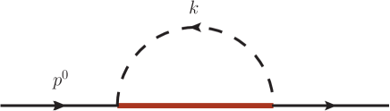
Figure 1: One-loop contribution to baryon self energy. The thick propagator indicates sum over all possible baryons that can contribute.

The leading 1-loop correction to the baryon self energy, diagram in Fig. 1, can be calculated through the matrix element $\langle{\bf B}\mid\delta\Sigma_{1-loop}\mid{\bf B}\rangle$, with:

$$\delta\Sigma_{1-loop} = i\,\frac{\mathring{g}_{A}^{2}}{F_{\pi}^{2}}\;\frac{1}{d-1}\;\sum_{n}G^{ia}{\cal{P}}_{n}G^{ia}\;I_{1-loop}(\delta m_{n}-p^{0},M_{\pi})\,,$$ (14)

where $n$ indicates the possible intermediate baryon spin-isospin states in the loop, ${\cal{P}}_{n}$ are the corresponding spin-flavor projection operators, $\delta m_{n}=\delta m(S_{n})$, and the loop integral is calculated in dimensional regularization with the result,

$$I_{1-loop}(Q,M_{\pi}) = \int\frac{d^{d}k}{(2\pi)^{d}}\;\frac{\vec{k}^{2}}{k^{2}-M_{\pi}^{2}+i\epsilon}\;\frac{1}{k^{0}-Q+i\epsilon}$$ (15)

$$= \frac{i}{16\pi^{2}}\left\{Q\;\left((3M_{\pi}^{2}-2Q^{2})(\lambda_{\epsilon}-\log\frac{M_{\pi}^{2}}{\mu^{2}})+(5M_{\pi}^{2}-4Q^{2})\right)\right.$$

$$+ 2\pi(M_{\pi}^{2}-Q^{2})^{3/2}+\left.4(Q^{2}-M_{\pi}^{2})^{3/2}\tanh^{-1}\frac{Q}{\sqrt{Q^{2}-M_{\pi}^{2}}}\right\}\,,$$

where $Q=\delta m_{n}-p^{0}$, $\lambda_{\epsilon}=\frac{1}{\epsilon}-\gamma+\log 4\pi$, and $\mu$ is the renormalization scale which will be taken later to be of the order of $m_{\rho}$. For the specific evaluation of $\delta\Sigma_{1-loop}$ for a given baryon state denoted by $in$, $p^{0}=\delta m_{in}-{\mathfrak{p}}^{0}$, where ${\mathfrak{p}}^{0}$ is a residual energy (when evaluated on an on-shell baryon it is the kinetic energy which is ${\cal{O}}(p^{2}/N_{c})$). The non-commutativity of the $1/N_{c}$ and Chiral expansions of course resides in the non-analytic terms of the loop integral through their dependence on the ratio $Q^{2}/M_{\pi}^{2}$. Notice that when the one loop integrals are written in terms of the residual momentum ${\mathfrak{p}}^{0}$, they do not depend on the spin-flavor singlet piece of $\delta m$, namely the $\sigma$-term in Eq.(5).

Appendix D provides all the necessary elements for the evaluation of the spin-flavor matrix elements in Eq. (14) as well as in the calculation of the one-loop corrections to the axial currents below. The explicit final expressions for the self energy are not given here because they are too lengthy, but with those elements the reader can easily obtain them.

The one-loop contribution to the wave function renormalization constant is given by:

$$\delta Z_{1-loop}=\left.\frac{\partial}{\partial{\mathfrak{p}}^{0}}\delta\Sigma_{1-loop}\right\arrowvert_{{{\mathfrak{p}}^{0}\to 0}}.$$ (16)

The explicit evaluation of the ultraviolet divergent pieces of the self energy gives:

$$\delta\Sigma_{1-loop}^{UV}=\frac{\lambda_{\epsilon}}{16\pi^{2}}\frac{\mathring{g}_{A}^{2}}{F_{\pi}^{2}}$$

$$\times \left\{\frac{C_{HF}}{24N_{c}}\left(-3M_{\pi}^{2}(3N_{c}(4+N_{c})-20\vec{S}^{2})+8\frac{C_{HF}^{2}}{N_{c}^{2}}(N_{c}(4+N_{c})(3+5\vec{S}^{2})-4\vec{S}^{2}(6+7\vec{S}^{2}))\right)\right.$$

$$+ \left.{\mathfrak{p}}^{0}\left(\frac{M_{\pi}^{2}}{2}(\frac{3}{8}N_{c}(4+N_{c})-\vec{S}^{2})-\frac{C_{HF}^{2}}{4N_{c}^{2}}(N_{c}(4+N_{c})(3+2\vec{S}^{2})-8\vec{S}^{2}(3+\vec{S}^{2}))\right)+{\cal{O}}({\mathfrak{p}}^{0}{{}^{{}^{2}}})\right\}.$$

The UV divergent pieces start at ${\cal{O}}(\xi^{2})$. Note that the UV divergencies in the mass (term independent of ${\mathfrak{p}}^{0}$) is produced by the contribution of the partner baryon and is proportional to the mass splitting. As is well known, they are absent in HBChPT without explicit $\Delta$. The ${\cal{O}}(N_{c}^{0})$ UV divergence is spin-flavor singlet and proportional to $M_{\pi}^{2}$, while the contributions to mass splittings are ${\cal{O}}(1/N_{c}^{2})$. Notice that the leading UV divergence of $\delta Z_{1-loop}$ is ${\cal{O}}(M_{\pi}^{2}N_{c})$: this is necessary as shown later for rendering the one-loop calculation of the axial currents consistent in the large $N_{c}$ limit. Since the calculation is accurate to ${\cal{O}}(\xi^{3})$, additional terms in the effective Lagrangian up to that order are necessary for renormalization. The terms necessary for renormalizing the self energy are therefore the following:

$${\cal{L}}_{\Sigma}^{CT} = {\bf B^{\dagger}}\left\{\frac{m_{1}(N_{c})}{N_{c}}+\frac{C_{HF1}(N_{c})}{N_{c}^{2}}\vec{S}^{2}+\frac{C_{HF2}(N_{c})}{N_{c}^{3}}\vec{S}^{4}\right.+\mu_{1}(N_{c})\chi_{+}+\frac{\mu_{2}(N_{c})}{N_{c}}\chi_{+}\vec{S}^{2}$$

$$+ \left.\left(\frac{w_{1}(N_{c})}{N_{c}}+\frac{w_{2}(N_{c})}{N_{c}}\vec{S}^{2}+\frac{w_{3}(N_{c})}{N_{c}^{3}}\vec{S}^{4}+(z_{1}(N_{c})N_{c}+\frac{z_{2}(N_{c})}{N_{c}}\vec{S}^{2})\chi_{+}\right)(iD_{0}-\delta m)\right\}{\bf B},$$

where the residual energy ${\mathfrak{p}}^{0}$ has been identified with the operator $(iD_{0}-\delta m)$. All LECs are here of the form $X(N_{c})=X_{0}+X_{1}/N_{c}+\cdots$. Writing $X=X(\mu)+\gamma_{{}_{X}}\lambda_{\epsilon}$, one renormalizes the self energy to ${\cal{O}}(\xi^{3})$. The coefficients $\gamma_{{}_{X}}$ are determined from $\delta\Sigma_{1-loop}^{UV}$ given above. While the counter-terms are defined such that $X(\mu)$ is ${\cal{O}}(N_{c}^{0})$, it is possible that $\gamma_{{}_{X}}$ is of higher order in $1/N_{c}$. Notice that among the higher order terms there are terms which can be simply absorbed into $1/N_{c}$ corrections to the LECs of the lowest order Lagrangian, and into $m_{0}$.

Finally, the baryon masses are given by:

$$m_{\bf B}=\langle{\bf B}\mid N_{c}{m}_{0}+\frac{C_{HF}}{N_{c}}\vec{S}^{2}+c_{1}N_{c}M_{\pi}^{2}+(\delta\Sigma^{UV~{}finite}_{1-loop}+\delta\Sigma^{CT})\arrowvert_{{\mathfrak{p}}^{0}=0}\;(1+\delta Z^{UV~{}finite}_{1-loop}+\delta Z^{CT})\mid{\bf B}\rangle.$$ (19)

Note that the correction to the wave function renormalization factor enters in the expression for the mass corrections: this is because $\delta\Sigma({\mathfrak{p}}^{0}=0)$ starts with terms ${\cal{O}}(\xi^{2})$ and $\delta Z$ starts at ${\cal{O}}(\xi)$, therefore the ${\cal{O}}(\xi^{3})$ terms of the mass correction involve these lower order terms of the wave function renormalization.

The one-loop corrections and corresponding counter-terms contribute to the masses at ${\cal{O}}(\xi^{2})$ and ${\cal{O}}(\xi^{3})$, while in a strict large $N_{c}$ limit the following ordering is found:

$$M_{B} = {\cal{O}}(N_{c})+{\cal{O}}(N_{c}M_{\pi}^{2})+{\cal{O}}(N_{c}^{0}M_{\pi})+\cdots~{}~{},$$

$$M_{B}-M_{B}^{\prime} = {\cal{O}}(\frac{1}{N_{c}})+{\cal{O}}(\frac{1}{M_{\pi}N_{c}^{2}}).$$ (20)

Obviously the term ${\cal{O}}(\frac{1}{M_{\pi}N_{c}^{2}})$ stems from the $1/N_{c}$ expansion of non-analytic terms and shows the non-commutativity of limits.

The one loop correction with the vertex proportional to $c_{1}$ in Eq.(6) gives ${\cal{O}}(\xi^{4})$ contributions to the masses, and is therefore beyond the accuracy considered here.

The $\sigma$-terms for $N$ and $\Delta$, defined by $\sigma_{B}=\hat{m}\frac{\partial m_{B}}{\partial\hat{m}}$ ($\hat{m}=\frac{1}{2}(m_{u}+m_{d})$), are ${\cal{O}}(\xi)$ with the one-loop corrections contributing up to ${\cal{O}}(\xi^{3})$. The difference $\sigma^{B}-\sigma^{B^{\prime}}$ is ${\cal{O}}(\xi^{2})$ and at that order it receives only finite contributions from the loop. This implies that the slopes of the $N$ and $\Delta$ masses as functions of $M_{\pi}$ are the same up to ${\cal{O}}(\xi^{2})$ deviations. This seems to be closely followed by the lattice QCD results analyzed later. In the large $N_{c}$ limit, obviously $\sigma={\cal{O}}(N_{c})$. The terms of that order are necessarily spin-flavor singlet, and taking the limit at fixed $M_{\pi}$ one finds $\sigma_{\Delta}-\sigma_{N}={\cal{O}}(1/N_{c}^{2})$, a result similar to the one in the $\xi$-expansion.

IV Axial couplings

In this section the evaluation of the axial couplings including corrections ${\cal{O}}(\xi^{2})$ is presented. At that order the one-loop corrections must be calculated.

The matrix elements of interest for the axial currents are $\langle{\bf B}^{\prime}\mid A^{ia}\mid{\bf B}\rangle$ evaluated at vanishing external 3-momentum. The axial couplings are then defined by:

$$\langle{\bf B}^{\prime}\mid A^{ia}\mid{\bf B}\rangle=g_{A}^{{\bf B}{\bf B}^{\prime}}\;\frac{5}{6}\;{\langle{\bf B}^{\prime}\mid G^{ia}\mid{\bf B}\rangle}\,.$$ (21)

The axial couplings defined here are ${\cal{O}}(N_{c}^{0})$. The ${\cal{O}}(N_{c})$ of the matrix elements of the axial currents is due to the operator $G^{ia}$. The factor $5/6$ mentioned earlier is included so that $g_{A}^{NN}$ at $N_{c}=3$ exactly corresponds to the usual nucleon $g_{A}$, which has the value $1.2701\pm 0.0025$ Beringer et al. (2012). This definition of the axial couplings is convenient in the context of the $1/N_{c}$ expansion, as the differences between the different axial couplings are ${\cal{O}}(1/N_{c}^{2})$.

Figure 2: Diagrams contributing to the 1-loop corrections to the axial-currents. The crossed circle denotes the axial-current operator.

The determination of the axial couplings to ${\cal{O}}(\xi^{2})$ require the calculation of the 1-loop corrections to the axial current. Only the contributions with no pion pole are necessary, and they are given by the diagrams in Fig. 2. The resulting 1-loop contribution to the axial currents reads:

$$\delta A^{ia}_{1-loop}=\delta A^{ia}_{1-loop}(1)+\delta A^{ia}_{1-loop}(2+3)+\delta A^{ia}_{1-loop}(4)\,,$$ (22)

where $\delta A^{ia}_{1-loop}(2+3)$ is given by a factor 1/2 times the no-baryon-pole contributions of diagrams (2+3). The different contributions read as follows, where one needs to take the limits ${\mathfrak{p}}^{0},{\mathfrak{p}^{\prime}}^{0}\to 0$:

$$\delta A^{ia}_{1-loop}(1) = {-}i\frac{\mathring{g}_{A}^{3}}{F_{\pi}^{2}}\frac{1}{d-1}$$

$$\times \sum_{n,n^{\prime}}G^{jb}{\cal{P}}_{n^{\prime}}G^{ia}{\cal{P}}_{n}G^{jb}\frac{I_{1-loop}(\delta m_{n}-p^{0},M_{\pi})-I_{1-loop}(\delta m_{n^{\prime}}-p^{\prime 0},M_{\pi})}{p^{0}-p^{\prime 0}-\delta m_{n}+\delta m_{n^{\prime}}},$$

$$\delta A^{ia}_{1-loop}(2+3) = \frac{\mathring{g}_{A}}{2}\left(G^{ia}\delta Z_{1-loop}+\delta Z_{1-loop}G^{ia}\right),$$

$$\delta A^{ia}_{1-loop}(4) = -\frac{\mathring{g}_{A}}{{3}F_{\pi}^{2}}\Delta(M_{\pi})G^{ia}.$$ (23)

Obviously, $G^{ia}$ and $\delta Z_{1-loop}$ do not commute in general. The pion tadpole integral in the last term is given by:

$$\Delta(M_{\pi})=-\frac{M_{\pi}^{2}}{16\pi^{2}}(\lambda_{\epsilon}-\log\frac{M_{\pi}^{2}}{\mu^{2}}).$$ (24)

Notice that the contribution by diagram (4) is actually ${\cal{O}}(\xi^{4})$, and thus beyond the degree of accuracy of the present calculation. It can serve however as a measure of the size of the NNNLO corrections.

The corrections to the axial currents must scale as ${\cal{O}}(N_{c}^{\nu})$ with $\nu\leq 1$. While diagram (4) is ${\cal{O}}(N_{c}^{0})$ and therefore consistent in itself, diagrams (1) and (2+3) above are ${\cal{O}}(N_{c}^{2})$. As shown in Ref. Flores-Mendieta et al. (1998), the offending terms cancel upon adding the diagrams. To test the cancellation it is sufficient to take the large $N_{c}$ limit at fixed $M_{\pi}$. A straightforward evaluation leads to:

$$\left(\delta A^{ia}_{1-loop}(1)+\delta A^{ia}_{1-loop}(2+3)\right){\Big{|}_{N_{c}\to\infty}}=-i\frac{\mathring{g}_{A}^{3}}{F_{\pi}^{2}}\frac{1}{d-1}\left\{\frac{1}{2}[[G^{jb},G^{ia}],G^{jb}]\frac{\partial}{\partial{{\mathfrak{p}}^{0}}}I_{1-loop}({\mathfrak{p}}^{0},M_{\pi})+\cdots\right\}\,,$$ (25)

where $\cdots$ indicate further terms which are consistent with the $N_{c}$ power counting. The suppression of the ${\cal{O}}(N_{c}^{2})$ terms is direct consequence of the appearance of the commutator of two generators $G$, which is ${\cal{O}}(N_{c}^{0})$, when the diagrams are added up. In consequence the displayed terms are ${\cal{O}}(N_{c}^{0})$.

The UV divergent contributions of the individual diagrams read:

$$\delta A^{ia}_{1-loop}(1)^{UV} = {-}\frac{\lambda_{\epsilon}}{48\pi^{2}}\frac{\mathring{g}_{A}^{3}}{F_{\pi}^{2}}\Big{\{}3M_{\pi}^{2}G^{jb}G^{ia}G^{jb}$$

$$- 2\left(\frac{C_{HF}}{N_{c}}\right)^{2}\Big{(}G^{jb}G^{ia}\left[\left[G^{jb},\vec{S}^{2}\right],\vec{S}^{2}\right]+\left[\vec{S}^{2},\left[\vec{S}^{2},G^{jb}\right]\right]G^{ia}G^{jb}$$

$$+ \left[\vec{S}^{2},G^{jb}\right]G^{ia}\left[G^{jb},\vec{S}^{2}\right]\Big{)}\Big{\}},$$

$$\delta A^{ia}_{1-loop}(2+3)^{UV} = \frac{\lambda_{\epsilon}}{96\pi^{2}}\frac{\mathring{g}_{A}^{3}}{F_{\pi}^{2}}\Big{\{}3M_{\pi}^{2}\{G^{ia},G^{2}\}$$

$$- 2\left(\frac{C_{HF}}{N_{c}}\right)^{2}\Big{(}G^{ia}G^{jb}[[G^{jb},\vec{S}^{2}],\vec{S}^{2}]+[\vec{S}^{2},[\vec{S}^{2},G^{jb}]G^{jb}G^{ia}\Big{)}\Big{\}},$$

$$\delta A^{ia}_{1-loop}(4)^{UV} = \frac{\lambda_{\epsilon}\,}{{48\pi^{2}}}\frac{\mathring{g}_{A}}{F_{\pi}^{2}}\;M_{\pi}^{2}\;G^{ia}.$$ (26)

One notices that only the terms proportional to $M_{\pi}^{2}$ in diagrams (1) and (2+3) diverge as proportional to $N_{c}^{2}$, while the terms proportional to $C_{HF}^{2}$ are ${\cal{O}}(N_{c}^{0})$. Thus, only the ${\cal{O}}(N_{c}^{2})$ terms proportional to $M_{\pi}^{2}$ need to be cancelled to give consistency. One can easily check that such a cancellation indeed occurs, leaving only terms ${\cal{O}}(N_{c}^{0})$. An explicit evaluation of these UV divergent terms using the results from Appendix D finally gives:

$$\delta{A^{ia}_{1-loop}}^{UV} = \frac{\lambda_{\epsilon}}{32\pi^{2}}\frac{\mathring{g}_{A}}{F_{\pi}^{2}N_{c}^{2}}\Big{\{}(\frac{2}{3}+\mathring{g}_{A}^{2})M_{\pi}^{2}N_{c}^{2}G^{ia}$$ (27)

$$+ \frac{C_{HF}^{2}\mathring{g}_{A}^{2}}{3}\Big{(}4-2N_{c}(4+N_{c})G^{ia}-7[\vec{S}^{2},[\vec{S}^{2},G^{ia}]]+4\{\vec{S}^{2},G^{ia}\}\Big{)}\Big{\}}.$$

The terms in the Lagrangian needed to renormalize the axial currents are then the following:

$${\cal{L}}{{}_{A}^{CT}}={\bf B^{\dagger}}u^{ia}\left(\frac{C^{A}_{0}}{N_{c}}G^{ia}+\frac{C^{A}_{1}}{4}\{\chi_{+},G^{ia}\}+\frac{C^{A}_{2}}{N_{c}^{2}}\{\vec{S}^{2},G^{ia}\}+\frac{C^{A}_{3}}{N_{c}}[\vec{S}^{2},G^{ia}]+\frac{C^{A}_{4}}{N_{c}}S^{i}I^{a}\right){\bf B}~{}.$$ (28)

These are all the terms which can contribute to the axial currents up to ${\cal{O}}(\xi)$, which will determine the axial couplings up to ${\cal{O}}(\xi^{2})$, i.e., NNLO, which is what is needed for our purpose. There are several very important observations concerning the $\xi$-power counting. The corrections to the axial couplings start at ${\cal{O}}(\xi)$, and the individual contributions of the different baryons in the loop diagrams are also ${\cal{O}}(\xi)$. Even the difference of different axial couplings $g_{A}^{BB^{\prime}}-g_{A}^{B^{\prime\prime}B^{\prime\prime\prime}}$ starts at ${\cal{O}}(\xi)$. These latter differences are UV finite. The large $N_{c}$ cancellations do not seem manifest. However, at $N_{c}=3$, where the $\xi$-expansion is used, cancellations do occur numerically as shown by Fig. 4 in Section V. Thus, the smallness of ${\cal{O}}(\xi)$ terms in the axial couplings is a result of the incipient manifestation of the cancellations in the large $N_{c}$ limit. If one would consider the strict large $N_{c}$ limit, the one loop corrections and counter-terms considered give the following $1/N_{c}$ power counting:

$$g_{A}^{BB^{\prime}}-\frac{5}{6}\mathring{g}_{A} = {\cal{O}}(M_{\pi}^{2})+\log\left(\frac{M_{\pi}^{2}}{\mu^{2}}\right){\cal{O}}(\frac{M_{\pi}^{2}}{N_{c}})+\cdots~{}~{},$$

$$g_{A}^{BB^{\prime}}-g_{A}^{B^{\prime\prime}B^{\prime\prime\prime}} = {\cal{O}}(\frac{1}{N_{c}^{2}})+{\cal{O}}(\frac{M_{\pi}}{N_{c}^{2}}),$$ (29)

where, as expected, the latter differences are UV finite as in the $\xi$ expansion.

The explicit expression for $g_{A}^{NN}$ at ${\cal{O}}(\xi^{2})$ is give here for completeness:

$$g_{A}^{NN} = \frac{5}{6}\mathring{g}_{A}+\frac{5}{12N_{c}^{2}}(3C^{A}_{2}+2N_{c}(C^{A}_{0}+C^{A}_{1}M_{\pi}^{2}N_{c}))$$ (30)

$$+ \frac{5\mathring{g}_{A}^{3}(4+N_{c})}{6C_{HF}F_{\pi}^{2}N_{c}^{2}(36\pi)^{2}}\left\{-18C_{HF}^{3}-12C_{HF}M_{\pi}^{2}N_{c}^{2}-9\pi C_{HF}^{2}\sqrt{-9C_{HF}^{2}+M_{\pi}^{2}N_{c}^{2}}\right.$$

$$+ 2\pi M_{\pi}^{2}N_{c}^{2}(M_{\pi}N_{c}-\sqrt{-9C_{HF}^{2}+M_{\pi}^{2}N_{c}^{2}}\;)+27C_{HF}^{3}\log\frac{M_{\pi}^{2}}{\mu^{2}}$$

$$+ \left.2\sqrt{9C_{HF}^{2}-M_{\pi}^{2}N_{c}^{2}}\;(9C_{HF}^{2}+2M_{\pi}^{2}N_{c}^{2})\tanh^{-1}\left(\frac{3C_{HF}}{\sqrt{9C_{HF}^{2}-M_{\pi}^{2}N_{c}^{2}}}\right)\right\}.$$

While in next section a discussion of the nucleon’s $g_{A}$ in the context of LQCD results is given, one can readily make an estimate of the spin-flavor symmetry breaking terms in the axial couplings $g_{A}^{NN}$ vs $g_{A}^{\Delta N}$ using the result for the $\Delta$ width:

$$\Gamma_{\Delta\to\pi N} = \frac{1}{12\pi}\left(\frac{6}{5}\frac{g_{A}^{\Delta N}}{F_{\pi}}\right)^{2}((m_{\Delta}-m_{N})^{2}-M_{\pi}^{2})^{3/2}.$$ (31)

Using the experimental value $\Gamma_{\Delta\to\pi N}(Exp)=116-120$ MeV Beringer et al. (2012), one obtains $g_{A}^{\Delta N}=1.235\pm 0.011$, which is remarkably close to $g_{A}^{NN}=1.2701\pm 0.0025$ Beringer et al. (2012).

V Analysis of lattice QCD results for baryon masses and the nucleon’s axial coupling

As an application of the present framework of the $\xi$-expansion, this section presents an analysis of LQCD results for baryon masses and the nucleon’s axial coupling.

Lattice QCD calculations of the non-strange ground state baryon masses (both of $N$ and $\Delta$ baryons) have opened the possibility of determining the quark mass dependencies, and similarly for the axial coupling of the nucleon. These calculations represent a very fruitful ground of applications for ChPT, allowing in particular for a study of the convergence of the low energy expansion. Current dynamical two- and three-light-flavor calculations of the hadron spectrum, and in particular of baryon masses, with fixed strange quark mass and variable $m_{u}=m_{d}$  Durr et al. (2008); Walker-Loud et al. (2009); Aoki et al. (2009); Lin et al. (2009); Aoki et al. (2010); Alexandrou et al. (2009); Aoki et al. (2011); Bietenholz et al. (2011) are achieving remarkably accurate results in a range of quark masses where extrapolations to the physical limit are now possible using effective theory. All calculations present similar results for the $N$ and $\Delta$ masses, namely, roughly linear dependencies of the masses as a function of $M_{\pi}$, and extrapolations to the correct physical value within a few percent. For the nucleon axial coupling $g_{A}^{NN}$ the results are particularly interesting  Edwards et al. (2006); Bratt et al. (2010); Alexandrou et al. (2011); Yamazaki et al. (2008, 2009); Lin et al. (2008) because they show small dependence in a broad range of $M_{\pi}$. The most recent LQCD calculations for $N_{f}=2$ Edwards et al. (2006); Lin et al. (2008); Alexandrou et al. (2011) and $N_{f}=2+1$ Yamazaki et al. (2008, 2009); Bratt et al. (2010), all agree on that observation. An open issue is that all calculations give an underestimation for the value of $g_{A}^{NN}$ of about $12\%$ below the experimental value.

Effects due to finite volume of the lattice have been studied for the observables considered here. Those effects are determined primarily by the value of the product $LM_{\pi}$, where $L$ is the length of the lattice. For the baryon masses, the rule $LM_{\pi}\gtrsim 4$ Alexandrou (2012) seems to be sufficient for the volume effects to be negligibly small. On the other hand, for $g_{A}^{NN}$ the LQCD understanding of the finite volume effects is not yet complete. According to Ref. Yamazaki et al. (2008), $g_{A}^{NN}$ clearly exhibits scaling in $LM_{\pi}$ and in lattices with $LM_{\pi}\sim 4-5$ the effect on $g_{A}^{NN}$ is a 9 % reduction in calculations with $2+1$ flavors of domain wall fermions and a 25 % reduction in calculations with two flavors of Wilson fermions. This has led to the current view that $LM_{\pi}\gtrsim 5-6$ or even higher may in fact be needed to reliably determine $g_{A}^{NN}$. Finite-volume effects for mases and the nucleon axial coupling have been studied in effective theories Beane and Savage (2004); Beane (2004); Colangelo et al. (2006); Khan et al. (2006); Bedaque et al. (2005); Detmold and Savage (2004); Smigielski and Wasem (2007); Ishikawa et al. (2009); Beane et al. (2011); Geng et al. (2011). A detailed study of these effects in the present formalism is beyond the scope of this work, and will be presented elsewhere Calle Cordón (work in preparation).

In the following, combined fits to LQCD results for $N$ and $\Delta$ masses and the nucleon $g_{A}$ as functions of $M_{\pi}$ are carried out. For the $N$ and $\Delta$ masses the results used are those from the PACS-CS collaboration of Ref. Aoki et al. (2009) and the LHP collaboration of Ref. Walker-Loud et al. (2009). For $g_{A}^{NN}$ the results used are those from the LHP collaboration Bratt et al. (2010) and from the ETM collaboration Alexandrou et al. (2011). All collaborations obtain results satisfying the constraint $LM_{\pi}\gtrsim 4$ and for quark masses reaching down close to the physical point, in particular for the baryon masses. The fits are carried out only including results where $LM_{\pi}\gtrsim 4$. The analysis of these LQCD results is carried out up to ${\cal{O}}(\xi^{3})$ for the masses and ${\cal{O}}(\xi^{2})$ for $g_{A}^{NN}$. The set of Lagrangian counter-terms is the one displayed in Eqs. (III) and (28), which are summarized by the following equations:

$$\delta\Sigma^{CT}({\mathfrak{p}}^{0}=0)(S) = \frac{m_{1}}{N_{c}}+\frac{C_{HF1}}{N_{c}^{2}}\vec{S}^{2}+\frac{C_{HF2}}{N_{c}^{3}}\vec{S}^{4}+\mu_{1}M_{\pi}^{2}+\frac{\mu_{2}}{N_{c}}\vec{S}^{2}M_{\pi}^{2}\,,$$

$$\delta Z^{CT}(S) = \frac{w_{1}}{N_{c}}+\frac{w_{2}}{N_{c}}\vec{S}^{2}+\frac{w_{3}}{N_{c}^{3}}\vec{S}^{4}+z_{1}N_{c}M_{\pi}^{2}+\frac{z_{2}}{N_{c}}\vec{S}^{2}M_{\pi}^{2}\,,$$

$$\delta g_{A}^{CT}(S,S^{\prime}) = \frac{C^{A}_{0}}{N_{c}}+C^{A}_{1}M_{\pi}^{2}+\frac{C^{A}_{2}}{N_{c}^{2}}(\vec{S}^{2}+\vec{S}^{\prime 2})+\frac{C^{A}_{3}}{N_{c}^{2}}(\vec{S}^{2}-\vec{S}^{\prime 2})$$ (32)

$$+ \frac{4C^{A}_{4}}{N_{c}(2+N_{c})}\delta_{SS^{\prime}}\vec{S}^{2}\,.$$

There are several LECs, which in order to be determined, require knowledge of results at different values of $N_{c}$. With the LQCD results at fixed $N_{c}=3$, those LECs combine with existing ones at lower order, making their determination impossible. Because LQCD results on $g_{A}^{N\Delta}$ are not analyzed and the lack of results for $g_{A}^{\Delta\Delta}$, LECs which split the values of the different $g_{A}$’s cannot be fixed either. For instance, the LECs $m_{1}$ and $w_{1}$ give the sub-leading $N_{c}$ dependence of $m_{0}$, and therefore at fixed $N_{c}=3$ they are absorbed into the fitted value of $m_{0}$. The same will happen with $C_{HF1}$ and $w_{2}$ with $C_{HF}$. The LEC $\mu_{1}$ is a correction to the LO $\sigma$-term LEC $c_{1}$. Similarly, one cannot separate $C^{A}_{0}$ from $\mathring{g}_{A}$. Therefore, without loss of generality at fixed $N_{c}=3$, the redundant LECs can be set to vanish. In addition, since the current fits only involve the nucleon’s axial coupling, $g_{A}^{NN}$, not all LECs affecting the axial currents can be determined as mentioned earlier. In particular, counter-terms with commutators in Eq. (28) only appear in $g_{A}^{N\Delta}$. Of course, depending on the order in the $\xi$-expansion, the number of LECs varies. Specifically, at leading order (LO), that is ${\cal{O}}(\xi)$ for the mass and ${\cal{O}}(\xi^{0})$ for the axial coupling, the LECs are $m_{0}$, $\mathring{g}_{A}$, $C_{HF}$ and $c_{1}$, at NLO the additional LECs $C_{HF1}$, $\mu_{1}$ and $C^{A}_{0}$ appear. Finally, at NNLO, that is ${\cal{O}}(\xi^{3})$ for the mass and ${\cal{O}}(\xi^{2})$ for the axial coupling, the additional LECs $\mu_{2}$, $z_{1}$ and $C^{A}_{1}$, which are fitted, and $\mu_{3}$, $w_{1}$, $w_{2}$ and $C^{A}_{2,3,4}$ that cannot be determined, make their appearance.

The combined fits to $N$ and $\Delta$ masses and to $g_{A}^{NN}$ up to NNLO for the four possible combinations of LQCD results from the collaborations considered here are presented in Table 1, which shows the values for LECs obtained from the fits and the extrapolated values for $m_{N}$, $m_{\Delta}$ and $g_{A}$ to the physical point. To estimate the theoretical errors, the original lattice results are bootstrapped by Montecarlo, and the errors correspond to a 68% confidence interval. In the fits, for the masses the range $M_{\pi}<600$ MeV is used while for the axial coupling of the nucleon the range $M_{\pi}<700$ MeV is used. It is expected that the radius of convergence of the low energy expansion is smaller for the baryon masses than for $g_{A}$; this is because in the latter case the discussed cancellations reduce the $M_{\pi}$ dependence, while the lack of such cancellations for the loop contribution to the masses is magnified by $N_{c}$. The combined fits are displayed in Fig 3, which shows the LO to NNLO fits of LQCD results from the PACS-CS and LHP collaborations.

LQCD Input	Order	$m_{0}$ [MeV]	$C_{HF}$ [MeV]	$\mathring{g}_{A}$	$c_{1}$ [MeV-1]	$\mu_{2}$ [MeV-1]	$z_{1}$ ($10^{-7}$) [MeV-2]	$C^{A}_{1}$ ($10^{-7}$)	$m_{N}$ [MeV]	$m_{\Delta}$ [MeV]	$g_{A}^{NN}$	$\chi^{2}$	$\chi^{2}/DOF$
PACS-CS $+$ LHP	LO	294 (4)	292 (10)	1.38 (1)	0.00048 (2)	-	-	-	981 (10)	1274 (10)	1.151 (8)	44	2.9
	NLO	262 (4)	191 (6)	1.38 (1)	0.00153 (2)	-	-	-	925 (10)	1162 (10)	1.124 (7)	74	4.9
	NNLO	264 (7)	170 (9)	1.43 (2)	0.00230 (7)	-0.0002 (1)	-9.0 (5)	-1.7 (6)	957 (14)	1195 (14)	1.131 (12)	40	3.3
LHP $+$ LHP	LO	308 (3)	335 (9)	1.38 (1)	0.000369 (12)	-	-	-	1028 (8)	1364 (10)	1.151 (8)	142	10.9
	NLO	264 (3)	216 (4)	1.38 (1)	0.00149 (2)	-	-	-	944 (8)	1217 (9)	1.120 (8)	145	11.2
	NNLO	237 (6)	212 (8)	1.43 (2)	0.00246 (6)	-0.00050 (9)	-5.0 (4)	-2.0 (6)	924 (12)	1219 (13)	1.117 (11)	56	5.6
PACS-CS $+$ ETM	LO	294 (4)	292 (10)	1.389 (9)	0.00048 (2)	-	-	-	982 (11)	1274 (11)	1.157 (8)	46	2.3
	NLO	262 (4)	190 (5)	1.387 (9)	0.00155 (2)	-	-	-	923 (10)	1161 (10)	1.131 (7)	77	3.9
	NNLO	263 (7)	167 (8)	1.47 (3)	0.00241 (9)	-0.0002 (1)	-9.3 (5)	-4 (2)	956 (14)	1192 (14)	1.16 (2)	40	2.4
LHP $+$ ETM	LO	308 (3)	335 (9)	1.39 (1)	0.00037 (1)	-	-	-	1029 (7)	1364 (9)	1.157 (9)	146	8.1
	NLO	264 (3)	215 (4)	1.39 (1)	0.00150 (2)	-	-	-	942 (8)	1215 (8)	1.127 (8)	149	8.3
	NNLO	235 (6)	209 (8)	1.45 (2)	0.00254 (8)	-0.00051 (8)	-5.1 (4)	-3.5 (1.4)	921 (12)	1214 (13)	1.134 (15)	58	3.9
Natural magnitude of LECs		$\sim 300$	$\sim 300$	1-2	$10^{-3}$	$10^{-3}$	$10^{-6}$	$10^{-6}$

Table 1: Results for LECs and extrapolated masses $m_{N}$ and $Re(m_{\Delta})$, and the nucleon $g_{A}$ from a combined fit to LQCD. The renormalization scale has been taken to be $\mu=700$ MeV. Lattice results for masses are from the PACS-CS Aoki et al. (2009) and LHP Walker-Loud et al. (2009) collaborations, and for $g_{A}^{NN}$ from LHP Walker-Loud et al. (2009); Bratt et al. (2010) and ETM Alexandrou et al. (2011) collaborations. Different orders in the $\xi$-expansion are shown. The LECs not shown have been set to vanish. Remark: the physical values of the baryon masses and $g_{A}^{NN}$ have been assigned errors of the same order as the theoretical error in the effective theory: $\sim\pm 20$ MeV for the $N$ and $\Delta$ masses, and $\sim\pm.03$ for $g_{A}^{NN}$.

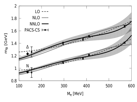
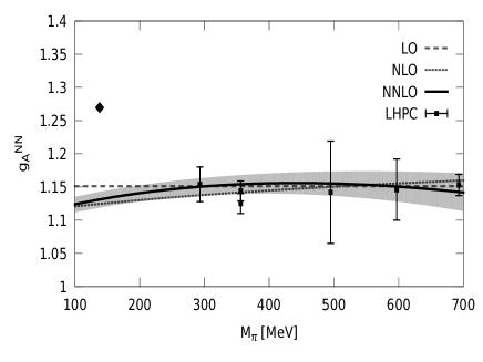
Figure 3: Combined fits to PACS-CS Aoki et al. (2009) and LHP Bratt et al. (2010) corresponding to the results shown in the first row of Table 1. The diamonds depict the physical values. The fits correspond to: LO (long-dashed line), NLO (short-dashed line) and NNLO (solid line). The bands correspond to the theoretical $68\%$ confidence interval.

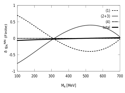
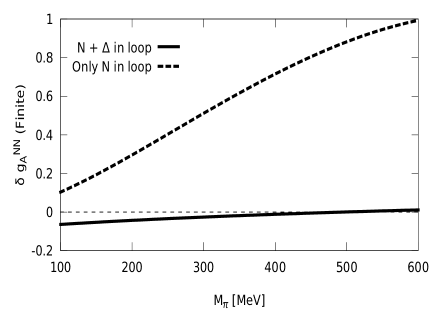
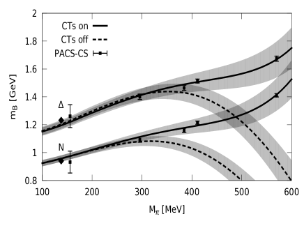
Figure 4: Finite parts of the one-loop contributions to $g_{A}^{NN}$: the upper left panel shows the individual contributions of the diagrams in Fig. 2 up to ${\cal{O}}(\xi^{3})$, and the right panel shows the effect of switching off the contribution of the $\Delta$ in the loops. The third panel shows the effect of removing the contributions of the counter-terms to the masses. Throughout $\mu=700$ MeV.

The following remarks on the fits are in order:

1. All fitted LECs are of natural size when the renormalization scale is taken to be $\mu\sim m_{\rho}$.

2. Parameters appearing at lower orders, namely $m_{0},~{}\mathring{g}_{A}$ and $C_{HF}$, remain stable at higher orders, except $c_{1}$ that changes by more than the estimated 30% when increasing the order in $\xi$ of the fit by one unit.

3. For baryon masses, LQCD data and physical point values are consistent even at LO, where with only three parameters one can extrapolate to the physical values and get a good fit up to $M_{\pi}\sim 350$ MeV as shown in Fig. 3. For larger values of $M_{\pi}$ an approximate linear fit is consistent Walker-Loud et al. (2009) in the range $M_{\pi}^{phys}<M_{\pi}<450$ MeV. Since at LO there are contributions to the baryon masses which are proportional to $N_{c}\,c_{1}M_{\pi}^{2}$, the NLO and NNLO effects are necessary to give the approximate linear behavior in that range of $M_{\pi}$.

4. For the case of the axial current, cancellations of large contributions from individual loop diagrams are very pronounced and the almost flat behavior of $g_{A}^{NN}$ as a function of $M_{\pi}$ obtained in LQCD is naturally explained. This is shown in the upper left panel of Fig. 4 which depicts the finite one-loop contributions to $g^{NN}_{A}$ from each diagram ($\mu=700$ MeV). As stated in Eq. (25) this cancellation is exact in the large $N_{c}$ limit. However, at $N_{c}=3$ this cancellation is not exact but still quite pronounced (solid curve in upper left panel of Fig. 4), and plays the key role in explaining the small dependence in $M_{\pi}$. A similar cancellation occurs between the contributions of $N$ and $\Delta$ in the loop contributions. This is shown in the upper right panel of Fig. 4.

5. The physical $g_{A}^{NN}$ cannot be fitted along with the lattice results, instead the lattice results and the expansion to NNLO extrapolate to a value 12% smaller than the physical one, as clearly shown in Fig. 3. The recent LQCD results Green et al. (2012) which reach further down in $M_{\pi}$ continue that trend. On the other hand, recent LQCD results for $g_{A}^{NN}$ from the CLS collaboration Capitani et al. (2012) can be made compatible with the physical value, but the error bars for $M_{\pi}<400$ MeV are quite large, and thus they cannot be considered to be significantly different than the ones of the LHP collaboration depicted in Fig. 3. It seems therefore, that the LQCD calculations are still evolving and it is possible that soon the origin of the mentioned discrepancy will be elucidated.

   The argument that the current LQCD results are correct and that the failure to extrapolate to the correct physical value is a problem of the effective theory seems unlikely on the following grounds. It is evident from Fig. 3 that in that case the effective theory should give up to a 12% enhancement below $M_{\pi}<300$ MeV. Since that does not occur at the order calculated here, namely NNLO, it should be provided by NNNLO contributions. The latter contributions are ${\cal{O}}(\xi^{3})$, and estimating that the effective value of the expansion parameter $\xi$ in the mass range of the physical pion mass is  1/3 to 1/4, one concludes that NNNLO corrections cannot be larger than a few percent.

6. A fit restricted only to masses gives too small a value for $g_{A}^{NN}$, namely, $g_{A}^{NN}\sim 0.5-0.8$. A realistic value can only be obtained with the combined fit.

7. Predictions for $g_{A}^{N\Delta}$ and $g_{A}^{\Delta\Delta}$ cannot be made without the corresponding LQCD results. However, the results at the physical point from Eq. (31) suggest that these are going to be very similar in value to $g_{A}^{NN}$. Further efforts to study these couplings in LQCD will be very useful.

8. In the masses one finds that above $M_{\pi}>350-400$ MeV there is a significant cancellation between the contributions of the one-loop diagram and the counter-terms as shown in Fig 4, which must be taken as an indicator of the range of convergence of the expansion. Note that the mass counter-terms are ${\cal{O}}(M_{\pi}^{2}N_{c}^{0})={\cal{O}}(\xi^{2})$.

9. Evaluating the $\sigma$ terms at the physical pion mass using the fits in Table 1, the results shown in Table 2 are obtained.

   LQCD Input	Order	$\sigma_{N}$ [MeV]	$\sigma_{\Delta}$ [MeV]
   PACS-CS $+$ LHP	LO	27	27
   	NLO	58	68
   	NNLO	66 (4)	90 (5)
   LHP $+$ LHP	LO	21	21
   	NLO	55	66
   	NNLO	76 (4)	99 (4)

   Table 2: Results for the $N$ and $\Delta$ $\sigma$-terms. These results correspond to the fits in the first two rows of Table 1.

   It is evident from the important change in the results from NLO to NNLO that the $\sigma$ terms cannot yet be very accurately determined from the current LQCD results. One finds that the $\sigma$ terms do not depend significantly on the choice of LQCD results for $g_{A}^{NN}$. $\sigma$ terms were obtained in other analyses of LQCD results in the framework of $SU(3)$ BChPT with $\Delta$ included in Ref. Martin Camalich et al. (2010). The present results at NLO are compatible with theirs, but are substantially larger at NNLO. However, if the fit is required to pass through the physical baryon masses, for $\sigma_{N}$ the NNLO is similar to that in Martin Camalich et al. (2010), however, the result obtained here where $\sigma_{N}<\sigma_{\Delta}$, is opposite to the one in Martin Camalich et al. (2010). This indicates that the $\sigma$ terms are sensitive to the particular formulation of the effective theory and also to the order of the expansion, an issue which remains to be clarified.

10. It must be emphasized that the results obtained here have many similarities with those obtained in works where the $\Delta$ has been included explicitly Procura et al. (2004); Bernard et al. (2005); Procura et al. (2006, 2007); Bernard (2008); Martin Camalich et al. (2010); Semke and Lutz (2012). The main advantage of the present approach of the $\xi$-expansion is its systematic character, which in particular will be more prominently shown when carrying out higher order calculations than the ones considered here.

VI Discussion and conclusions

Chiral symmetry and the large $N_{c}$ limit are of fundamental conceptual importance in QCD. The former is known to play a crucial role in light hadrons, and there are multiple indications that the latter is also important, in particular for baryons. It is therefore very important to have a theoretical framework where both of these aspects of QCD are consistently incorporated. This is possible with the combined $1/N_{c}$ and Chiral expansions of QCD, which in the baryon sector is implemented with the effective theory discussed in this work. A particular power counting, the $\xi$-expansion, which links the $1/N_{c}$ and low energy expansions as $1/N_{c}={\cal{O}}(\xi)={\cal{O}}(p)$ is proposed as the most realistic one for studying baryons at $N_{c}=3$. Results for the masses and axial couplings at NNLO have been given, and applied to current LQCD results.

The $\xi$-expansion at NNLO clearly provides a satisfactory description of the LQCD results, and in particular it illuminates the mild dependence of the axial couplings on the quark masses as a result of important cancellations, which had been realized in various previous analysis by various groups. It is important to complete the study in $SU(3)$, in particular because the one-loop contributions to the baryon masses become larger in magnitude, and a smaller range of convergence is expected Semke and Lutz (2012). These results will be presented elsewhere Calle Cordón and Goity (work in preparation). Recently, results for the axial currents with three flavors in a similar framework to the one developed here were presented in Ref. Flores-Mendieta et al. (2012).

The deficit in $g_{A}^{NN}$ at the physical point is expected to be a LQCD issue rather than a problem of convergence of the effective theory. The main reason for this expectation is that the $\xi$ expansion is especially well behaved for $g_{A}$. Among the possible sources of systematic errors in the extraction of $g_{A}$ from LQCD calculations might be the finite volume effects and/or the contamination in the three-point functions by excited baryon states.

In addition to the tests LQCD can provide on quark mass dependencies, it is also an ideal tool to test the $N_{c}$ behavior of QCD. Baryon LQCD is becoming accessible at varying values of $N_{c}$ DeGrand (2012), which is a promising development.

Appendix A Spin-flavor Algebra

The $4N_{f}^{2}-1$ generators of the spin-flavor group $SU(2N_{f})$ consist of the three spin generators $S^{i}$, the $N_{f}^{2}-1$ flavor $SU(N_{f})$ generators $T^{a}$, and the remaining $3(N_{f}^{2}-1)$ spin/flavor generators $G^{ia}$. The commutation relations are:

$$[S^{i},S^{j}]=i\epsilon_{ijk}S^{k},~{}~{}[T^{a},T^{b}]=if_{abc}T^{c},~{}~{}[T^{a},S^{i}]=0$$ ,

$$[S^{i},G^{ja}]=i\epsilon_{ijk}G^{ka},~{}~{}[T^{a},G^{ib}]=if_{abc}G^{ic}$$ ,

$$[G^{ia},G^{jb}]=\frac{i}{4}\delta^{ij}f^{abc}T^{c}+\frac{i}{2N_{f}}\delta^{ab}\epsilon^{ijk}S^{k}+\frac{i}{2}\epsilon^{ijk}d^{abc}G^{kc}$$ . (33)

For two flavors one has the isospin generators $I^{a}$ $a=1,2,3$.

In representations with $N_{c}$ indices (baryons), the generators $G^{ia}$ have matrix elements ${\cal{O}}(N_{c})$ on states with $S={\cal{O}}(N_{c}^{0})$. A contracted $SU(4)$ algebra is defined by the generators $\{S^{i},I^{a},X^{ia}\}$, where $X^{ia}=G^{ia}/N_{c}$. In large $N_{c}$, the generators $X^{ia}$ become semiclassical as $[X^{ia},X^{jb}]={\cal{O}}(1/N_{c}^{2})$, while having matrix elements ${\cal{O}}(1)$ in baryon representations.

Appendix B Non-linear realization of chiral symmetry and spin-flavor transformations

In the symmetric representations of $SU(4)$ the baryon spin-flavor multiplet consists of the baryon states with $I=S$. In particular, isospin transformations will act on the spin-flavor multiplet in an obvious way. This permits a straightforward implementation of the non-linear realization of chiral $SU_{L}(2)\times SU_{R}(2)$ on the spin-flavor multiplet. Defining as usual the Goldstone Boson fields $\pi^{a}$ through the unitary parametrization $u=\exp(i\frac{\pi^{a}I^{a}}{F_{\pi}})$ (note that in the fundamental representation $I^{a}=\tau^{a}/2$), for any isospin representation one defines a non-linear realization of chiral symmetry according to Coleman et al. (1969); Callan et al. (1969):

$$(L,R):u=u^{\prime}=Ruh^{\dagger}(L,R,u)=h(L,R,u)uL^{\dagger},$$ (34)

where $(L,R)$ is a $SU_{L}(2)\times SU_{R}(2)$ transformation. This equation defines $h$, and since $h$ is an isospin $SU(2)$ transformation itself, it can be written as $h=\exp(ic^{a}I^{a})$. The chiral transformation on the baryon multiplet ${\bf B}$ is then given by:

$$(L,R):{\bf B}={\bf B}^{\prime}=h(L,R,u){\bf B}.$$ (35)

On the other hand, spin-flavor transformations of interest are the contracted ones, namely those generated by $\{S^{i},I^{a},X^{ia}=\frac{1}{N_{c}}G^{ia}\}$. While the isospin transformations act on the pion fields in the usual way, and the spin transformations must be performed along with the corresponding spatial rotations. The transformations generated by $X^{ia}$ are defined to only act on the baryons.

Appendix C Tools for building effective Lagrangians

The effective baryon Lagrangian can be expressed in the usual way as a series of terms which are $SU_{L}(2)\times SU_{R}(2)$ invariant (upon introduction of appropriate sources; see for instance Scherer (2003) for details). In addition, implemented in the effective Lagrangian is the approximate $SU(4)$ symmetry and its breaking as a power series in $1/N_{c}$ Jenkins (1996). The fields in the effective Lagrangian are the Goldstone Bosons parametrized by the unitary $SU(2)$ matrix field $u$ and the baryons given by the symmetric $SU(4)$ multiplet ${\bf B}$ of $I=S$ fields.

The building blocks for the effective theory consist of low energy operators, and spin-flavor operators.

The low energy operators are the usual ones, namely:

$$D_{\mu} = \partial_{\mu}-i\Gamma_{\mu},~{}~{}~{}\Gamma_{\mu}=\Gamma_{\mu}^{\dagger}=\frac{1}{2}(u^{\dagger}(i\partial_{\mu}+r_{\mu})u+u(i\partial_{\mu}+\ell_{\mu})u^{\dagger}),$$

$$u_{\mu} = u^{\dagger}_{\mu}=u^{\dagger}(i\partial_{\mu}+r_{\mu})u-u(i\partial_{\mu}+\ell_{\mu})u^{\dagger},$$

$$\chi = 2B_{0}(s+ip),~{}~{}\chi_{\pm}=u^{\dagger}\chi u^{\dagger}\pm u\chi^{\dagger}u,$$

$$F^{\mu\nu}_{L} = \partial^{\mu}\ell^{\nu}-\partial^{\nu}\ell^{\mu}-i[\ell^{\mu},\ell^{\nu}],~{}~{}F^{\mu\nu}_{R}=\partial^{\mu}r^{\nu}-\partial^{\nu}r^{\mu}-i[r^{\mu},r^{\nu}],$$ (36)

where $D_{\mu}$ is the chiral covariant derivative, $s$ and $p$ are scalar and pseudo-scalar sources, $\chi_{\pm}=2M_{\pi}^{2}+\cdots$, and $\ell_{\mu}$ and $r_{\mu}$ are gauge sources. The spin-flavor operators are tensor operators consisting of products of the spin-flavor generators. These operators can be reduced by means of the commutation relations to forms which only contain anti-commutators. A set of identities shown in Table 3 permits one to arrive at sets of basis operators at each order in $1/N_{c}$ for a given spin/isospin tensor type of operator. The $1/N_{c}$ order $\nu_{O}$ of an operator $O$, reduced as mentioned, is $\nu_{O}=n-1-\kappa$ Dashen et al. (1995), where $n$ is the number of generators appearing as factors in the operator (one then says that the operator is an $n$-body operator), and $\kappa$ is the number of generators $G^{ia}$ in the product.

The leading order equations of motion can be used in the construction of the higher order terms, namely, $iD_{0}{\bf B}=(\frac{C_{HF}}{N_{c}}S(S+1)+\frac{c_{1}}{2}N_{c}\chi_{+}){\bf B}$, and $\nabla_{\mu}u^{\mu}=\frac{i}{2}\chi_{-}$.

Appendix D Matrix elements of spin-flavor operators in the symmetric representations of ${\mathbf{SU(4)}}$

The evaluation of the matrix elements of spin-flavor operators in the present work can be carried out starting from the following matrix elements of the spin-flavor generators in the totally symmetric representation of $SU(4)$ corresponding to the Young tableux with a single row of $N_{c}$ boxes. The basis states of the symmetric representation consists of the states with $I=S$, namely $\mid S\,S_{3}I_{3}\rangle$, where $S_{3}$ and $I_{3}$ are the spin and isospin projections respectively.

$$\langle S^{\prime}\,S^{\prime}_{3}I^{\prime}_{3}\mid S^{i}\mid S\,S_{3}I_{3}\rangle = \sqrt{S(S+1)}\delta_{SS^{\prime}}\delta_{I_{3}I^{\prime}_{3}}\langle S\,S_{3},1i\mid S^{\prime}\,S^{\prime}_{3}\rangle,$$

$$\langle S^{\prime}\,S^{\prime}_{3}I^{\prime}_{3}\mid I^{a}\mid S\,S_{3}I_{3}\rangle = \sqrt{S(S+1)}\delta_{SS^{\prime}}\delta_{S_{3}S^{\prime}_{3}}\langle S\,I_{3},1a\mid S^{\prime}I^{\prime}_{3}\rangle,$$

$$\langle S^{\prime}\,S^{\prime}_{3}I^{\prime}_{3}\mid G^{ia}\mid S\,S_{3}I_{3}\rangle = \frac{1}{4}\sqrt{\frac{2S+1}{2S^{\prime}+1}}\zeta(N_{c},S,S^{\prime})\langle S\,S_{3},1i\mid S^{\prime}\,S^{\prime}_{3}\rangle\langle S\,I_{3},1a\mid S^{\prime}I^{\prime}_{3}\rangle,$$ (37)

where $\zeta(N_{c},S,S^{\prime})=\sqrt{(2+N_{c})^{2}-(S-S^{\prime})^{2}(S+S^{\prime}+1)^{2}}$ Carlson et al. (1999). The products of generators can be reduced by means of the use of the commutation relations, and further, for matrix elements in the symmetric representation, via the reduction rules Dashen et al. (1995), which for convenience are displayed in Table 3.

Table 3: $SU(4)$ operator identities in the totally symmetric irreducible representation $(N_{c},0,0)$ of $SU(4)$. The last column gives the operator’s quantum numbers $(J,I)$ under $SU(2)\times SU(2)$

$\{S^{i},S^{i}\}-\{I^{a},I^{a}\}=0$	(0,0)
$\{S^{i},S^{i}\}+\{I^{a},I^{a}\}+4\{G^{ia},G^{ia}\}=\frac{3}{2}N_{c}(4+N_{c})$	(0,0)
$2\{S^{i},G^{ia}\}=(2+N_{c})I^{a}$	(0,1)
$2\{I^{a},G^{ia}\}=(2+N_{c})S^{i}$	(1,0)
$\frac{1}{2}\{S^{k},I^{c}\}-\epsilon^{ijk}\epsilon^{abc}\{G^{ia},G^{jb}\}=(2+N_{c})G^{kc}$	(1,1)
$\epsilon^{ijk}\{S^{i},G^{jc}\}=\epsilon^{abc}\{I^{a},G^{kb}\}$	(1,1)
$4\{G^{ia},G^{ib}\}\arrowvert_{I=2}=\{I^{a},I^{b}\}\arrowvert_{I=2}$	(0,2)
$4\{G^{ia},G^{ja}\}\arrowvert_{J=2}=\{S^{i},S^{j}\}\arrowvert_{J=2}$	(2,0)

Useful matrix elements:

It is always convenient to express matrix elements in terms of reduced matrix elements (RMEs) defined in the ordinary Wigner-Eckart fashion Edmonds (1955). The RMEs defined here are with respect to $SU_{\rm spin}(2)\times SU_{I}(2)$. For matrix elements in the symmetric representation of spin-flavor the Wigner-Eckart theorem reads:

$$\langle S^{\prime}\,S^{\prime}_{3}I^{\prime}_{3}\mid{\mathbf{O}}^{\mathbf{JJ_{3}}}_{\mathbf{II_{3}}}\mid S\,S_{3}I_{3}\rangle=\frac{\langle S^{\prime}\mid\mid{\mathbf{O}}^{\mathbf{J}}_{\mathbf{I}}\mid\mid S\rangle}{2S^{\prime}+1}\langle SS_{3},{\mathbf{JJ_{3}}}\mid S^{\prime}S^{\prime}_{3}\rangle\langle SI_{3},{\mathbf{II_{3}}}\mid S^{\prime}I^{\prime}_{3}\rangle,$$ (38)

where ${\mathbf{O}}$ is an $SU_{S}(2)\times SU_{I}(2)$ irreducible tensor operator, and $\langle S^{\prime}\mid\mid{\mathbf{O}}^{\mathbf{J}}_{\mathbf{I}}\mid\mid S\rangle$ is the reduced matrix element. Note that the notation $\mid\mid S\rangle$ indicates the spin-flavor states in the symmetric representation $(N_{c},0,0)$ with $I=S$. The reduced matrix elements of the $SU(4)$ generators read:

$$\langle S^{\prime}\mid\mid S\mid\mid S\rangle = \delta_{SS^{\prime}}(2S+1)\sqrt{S(S+1)},$$

$$\langle S^{\prime}\mid\mid I\mid\mid S\rangle = \delta_{SS^{\prime}}(2S+1)\sqrt{S(S+1)},$$

$$\langle S^{\prime}\mid\mid G\mid\mid S\rangle = \delta_{\{S,S^{\prime},1\}}\frac{1}{4}\sqrt{(2S+1)(2S^{\prime}+1)}\zeta(N_{c},S,S^{\prime}),$$ (39)

where $\delta_{\{S,S^{\prime},1\}}=1$ if $\mid S-S^{\prime}\mid\leq 1$ and otherwise vanishes.

Reduced matrix elements of the operators involving the projects ${\cal{P}}_{n}$ are easily obtained using that ${\cal{P}}_{n}=\sum_{S_{n3},I_{n3}}\mid S_{n},S_{n3}I_{n3}\rangle\langle S_{n},S_{n3}I_{n3}\mid$, and the $SU(2)$ re-coupling results Edmonds (1955). For the masses the relevant such RME becomes:

$$\langle S\mid\mid G^{ia}{\cal{P}}_{n}G^{ia}\mid\mid S\rangle=\frac{1}{2S+1}\langle S_{n}\mid\mid G\mid\mid S\rangle^{2}.$$ (40)

For the axial currents the following RME is needed, namely:

$$\langle S^{\prime}\mid\mid G^{jb}{\cal{P}}_{n^{\prime}}G^{ia}{\cal{P}}_{n}G^{jb}\mid\mid S\rangle = \left\{\begin{array}[]{ccc}S&S_{n}&1\\ S_{n^{\prime}}&S^{\prime}&1\end{array}\right\}^{2}$$ (43)

$$\times \langle S^{\prime}\mid\mid G\mid\mid S_{n^{\prime}}\rangle\langle S_{n^{\prime}}\mid\mid G\mid\mid S_{n}\rangle\langle S_{n}\mid\mid G\mid\mid S\rangle.$$ (44)

Various reduced matrix elements which appear in the evaluation of the UV divergent pieces of the one-loop contributions to the self energy and to the axial currents are given below. They are obtained using the results given in the above Eqs. (40) and (44):

$$\langle S^{\prime}\mid\mid G^{2}\mid\mid S\rangle=\frac{1}{2}\delta_{SS^{\prime}}(2S+1)(-S(S+1)+\frac{3}{8}N_{c}(4+N_{c})),$$ (45)

where $G^{2}=G^{ia}G^{ia}$.

$$\langle S^{\prime}\mid\mid G\vec{S}^{2}G\mid\mid S\rangle=\frac{1}{2}\delta_{SS^{\prime}}(2S+1)\left(\frac{3}{4}N_{c}(4+N_{c})+\frac{1}{8}(-40+12N_{c}+3N_{c}^{2})S(S+1)-(S(S+1))^{2}\right),$$ (46)

$$\langle S^{\prime}\mid\mid G\vec{S}^{4}G\mid\mid S\rangle = \frac{1}{2}\delta_{SS^{\prime}}(2S+1)\left(\frac{3}{4}N_{c}(4+N_{c})+(-6+5N_{c}+\frac{5}{4}N_{c}^{2})S(S+1)\right.$$ (47)

$$+ \left.(-7+\frac{3}{4}N_{c}+\frac{3}{16}N_{c}^{2})(S(S+1))^{2}-\frac{1}{2}(S(S+1))^{3}\right).$$

In the following, $S^{\prime}=S$ or $S\pm 1$. With obvious notation:

$$\langle S^{\prime}\mid\mid\{S^{i},G^{ia}\}\mid\mid S\rangle=\delta_{SS^{\prime}}(1+\frac{N_{c}}{2})(2S+1)\sqrt{S(S+1)},$$ (48)

obtained using the corresponding reduction relation in Table 3.

$$\langle S^{\prime}\mid\mid S^{i}I^{a}\mid\mid S\rangle=\delta_{SS^{\prime}}(2S+1)S(S+1),$$ (49)

$$\langle S^{\prime}\mid\mid SG^{ia}S\mid\mid S\rangle=\frac{1}{2}(S(S+1)+S^{\prime}(S^{\prime}+1)-2)\langle S^{\prime}\mid\mid G\mid\mid S\rangle,$$ (50)

$$\langle S^{\prime}\mid\mid GG^{ia}G\mid\mid S\rangle = \frac{1}{16}\langle S^{\prime}\mid\mid G\mid\mid S\rangle$$ (51)

$$\times \left(3N_{c}(4+N_{c})-4(2+S(S+1)+S^{\prime}(S^{\prime}+1))\right),$$

$$\langle S^{\prime}\mid\mid GG^{ia}\vec{S}^{2}G\mid\mid S\rangle = \frac{1}{2}\langle S^{\prime}\mid\mid G\mid\mid S\rangle\left(\frac{3}{4}N_{c}(4+N_{c})\right.$$ (52)

$$+ \left.S(S+1)(-S(S+1)-5+\frac{3}{8}N_{c}(4+N_{c})+\frac{1}{2}S^{\prime}(S^{\prime}+1))\right.$$

$$- \left.S^{\prime}(S^{\prime}+1)(1+\frac{1}{2}S^{\prime}(S^{\prime}+1))\right),$$

$$\langle S^{\prime}\mid\mid GG^{ia}\vec{S}^{4}G\mid\mid S\rangle = \frac{1}{2}\langle S^{\prime}\mid\mid G\mid\mid S\rangle$$ (53)

$$\times \left(\frac{3}{2}N_{c}(4+N_{c})+(S(S+1))^{2}(-16+\frac{3}{8}N_{c}(4+N_{c})-3S^{\prime}(S^{\prime}+1))\right.$$

$$+ \left.(S^{\prime}(S^{\prime}+1))^{2}(1-\frac{3}{2}S^{\prime}(S^{\prime}+1))\right.$$

$$+ \left.S(S+1)(-12+\frac{5}{2}N_{c}(4+N_{c})+\frac{7}{2}(S^{\prime}(S^{\prime}+1))^{2})\right),$$

$$\langle S^{\prime}\mid\mid G\vec{S}^{2}G^{ia}\vec{S}^{2}G\mid\mid S\rangle = \frac{1}{4}\langle S^{\prime}\mid\mid G\mid\mid S\rangle$$ (54)

$$\times \left((2+N_{c})^{2}+\frac{1}{2}(-16+5N_{c}(4+N_{c}))(S(S+1)+S^{\prime}(S^{\prime}+1))\right.$$

$$- (S(S+1))^{2}(9+S(S+1))-(S^{\prime}(S^{\prime}+1))^{2}(9+S^{\prime}(S^{\prime}+1))$$

$$+ \left.\frac{3}{4}(-16+N_{c}(4+N_{c}))S(S+1)S^{\prime}(S^{\prime}+1)\right).$$

Finally, using that for any spin and isospin singlet operator (not necessarily an $SU(4)$ singlet) ${\cal{Q}}$, $\langle S^{\prime}\mid\mid{\cal{Q}}{\mathbf{O^{J}_{I}}}\mid\mid S\rangle=\frac{1}{2S^{\prime}+1}\langle S^{\prime}\mid\mid{\cal{Q}}\mid\mid S^{\prime}\rangle\langle S^{\prime}\mid\mid{\mathbf{O^{J}_{I}}}\mid\mid S\rangle$, one can easily obtain the rest of the matrix elements involved in the calculation of the axial currents.

References

- Pagels (1975) H. Pagels, Phys.Rept. 16, 219 (1975).
- Weinberg (1968) S. Weinberg, Phys.Rev. 166, 1568 (1968).
- Coleman et al. (1969) S. R. Coleman, J. Wess, and B. Zumino, Phys.Rev. 177, 2239 (1969).
- Callan et al. (1969) C. G. Callan, S. R. Coleman, J. Wess, and B. Zumino, Phys.Rev. 177, 2247 (1969).
- Gasser et al. (1988) J. Gasser, M. Sainio, and A. Svarc, Nucl.Phys. B307, 779 (1988).
- Bernard et al. (1995) V. Bernard, N. Kaiser, and U.-G. Meissner, Int.J.Mod.Phys. E4, 193 (1995), eprint hep-ph/9501384.
- Jenkins and Manohar (1991a) E. E. Jenkins and A. V. Manohar, Phys.Lett. B255, 558 (1991a).
- Ellis and Tang (1998) P. J. Ellis and H.-B. Tang, Phys.Rev. C57, 3356 (1998), eprint hep-ph/9709354.
- Becher and Leutwyler (1999) T. Becher and H. Leutwyler, Eur.Phys.J. C9, 643 (1999), eprint hep-ph/9901384.
- Fuchs et al. (2003) T. Fuchs, J. Gegelia, G. Japaridze, and S. Scherer, Phys.Rev. D68, 056005 (2003), eprint hep-ph/0302117.
- Hemmert et al. (1997) T. R. Hemmert, B. R. Holstein, and J. Kambor, Phys.Lett. B395, 89 (1997), eprint hep-ph/9606456.
- Hemmert et al. (1998) T. R. Hemmert, B. R. Holstein, and J. Kambor, J.Phys.G G24, 1831 (1998), eprint hep-ph/9712496.
- Hemmert et al. (2003) T. R. Hemmert, M. Procura, and W. Weise, Phys.Rev. D68, 075009 (2003), eprint hep-lat/0303002.
- Fettes and Meissner (2001) N. Fettes and U. G. Meissner, Nucl.Phys. A679, 629 (2001), eprint hep-ph/0006299.
- Procura et al. (2006) M. Procura, B. Musch, T. Wollenweber, T. Hemmert, and W. Weise, Phys.Rev. D73, 114510 (2006), eprint hep-lat/0603001.
- Hacker et al. (2005) C. Hacker, N. Wies, J. Gegelia, and S. Scherer, Phys.Rev. C72, 055203 (2005), eprint hep-ph/0505043.
- Bernard et al. (2003) V. Bernard, T. R. Hemmert, and U.-G. Meissner, Phys.Lett. B565, 137 (2003), eprint hep-ph/0303198.
- Bernard et al. (2005) V. Bernard, T. R. Hemmert, and U.-G. Meissner, Phys.Lett. B622, 141 (2005), eprint hep-lat/0503022.
- Procura et al. (2007) M. Procura, B. Musch, T. Hemmert, and W. Weise, Phys.Rev. D75, 014503 (2007), eprint hep-lat/0610105.
- ’t Hooft (1974) G. ’t Hooft, Nucl.Phys. B72, 461 (1974).
- Witten (1979) E. Witten, Nucl.Phys. B160, 57 (1979).
- Gervais and Sakita (1984a) J.-L. Gervais and B. Sakita, Phys.Rev.Lett. 52, 87 (1984a).
- Gervais and Sakita (1984b) J.-L. Gervais and B. Sakita, Phys.Rev. D30, 1795 (1984b).
- Dashen and Manohar (1993a) R. F. Dashen and A. V. Manohar, Phys.Lett. B315, 425 (1993a), eprint hep-ph/9307241.
- Dashen and Manohar (1993b) R. F. Dashen and A. V. Manohar, Phys.Lett. B315, 438 (1993b), eprint hep-ph/9307242.
- Jenkins (1996) E. E. Jenkins, Phys.Rev. D53, 2625 (1996), eprint hep-ph/9509433.
- Flores-Mendieta et al. (1998) R. Flores-Mendieta, E. E. Jenkins, and A. V. Manohar, Phys.Rev. D58, 094028 (1998), eprint hep-ph/9805416.
- Flores-Mendieta and Hofmann (2006) R. Flores-Mendieta and C. P. Hofmann, Phys.Rev. D74, 094001 (2006), eprint hep-ph/0609120.
- Cohen and Broniowski (1992) T. D. Cohen and W. Broniowski, Phys.Lett. B292, 5 (1992), eprint hep-ph/9208253.
- Hagler (2010) P. Hagler, Phys.Rept. 490, 49 (2010), eprint 0912.5483.
- Fodor and Hoelbling (2012) Z. Fodor and C. Hoelbling, Rev.Mod.Phys. 84, 449 (2012), eprint 1203.4789.
- Alexandrou (2012) C. Alexandrou, Prog.Part.Nucl.Phys. 67, 101 (2012), eprint 1111.5960.
- Durr et al. (2008) S. Durr, Z. Fodor, J. Frison, C. Hoelbling, R. Hoffmann, et al., Science 322, 1224 (2008), eprint 0906.3599.
- Walker-Loud et al. (2009) A. Walker-Loud, H.-W. Lin, D. Richards, R. Edwards, M. Engelhardt, et al., Phys.Rev. D79, 054502 (2009), eprint 0806.4549.
- Aoki et al. (2009) S. Aoki et al. (PACS-CS Collaboration), Phys.Rev. D79, 034503 (2009), eprint 0807.1661.
- Aoki et al. (2010) S. Aoki et al. (PACS-CS Collaboration), Phys.Rev. D81, 074503 (2010), eprint 0911.2561.
- Aoki et al. (2011) Y. Aoki et al. (RBC Collaboration, UKQCD Collaboration), Phys.Rev. D83, 074508 (2011), eprint 1011.0892.
- Bietenholz et al. (2011) W. Bietenholz, V. Bornyakov, M. Gockeler, R. Horsley, W. Lockhart, et al., Phys.Rev. D84, 054509 (2011), eprint 1102.5300.
- Lin et al. (2009) H.-W. Lin et al. (Hadron Spectrum Collaboration), Phys.Rev. D79, 034502 (2009), eprint 0810.3588.
- Alexandrou et al. (2009) C. Alexandrou et al. (ETM Collaboration), Phys.Rev. D80, 114503 (2009), eprint 0910.2419.
- Edwards et al. (2006) R. Edwards et al. (LHPC Collaboration), Phys.Rev.Lett. 96, 052001 (2006), eprint hep-lat/0510062.
- Bratt et al. (2010) J. Bratt et al. (LHPC Collaboration), Phys.Rev. D82, 094502 (2010), eprint 1001.3620.
- Alexandrou et al. (2011) C. Alexandrou et al. (ETM Collaboration), Phys.Rev. D83, 045010 (2011), eprint 1012.0857.
- Yamazaki et al. (2008) T. Yamazaki et al. (RBC+UKQCD Collaboration), Phys.Rev.Lett. 100, 171602 (2008), eprint 0801.4016.
- Yamazaki et al. (2009) T. Yamazaki, Y. Aoki, T. Blum, H.-W. Lin, S. Ohta, et al., Phys.Rev. D79, 114505 (2009), eprint 0904.2039.
- Lin et al. (2008) H.-W. Lin, T. Blum, S. Ohta, S. Sasaki, and T. Yamazaki, Phys.Rev. D78, 014505 (2008), eprint 0802.0863.
- Jenkins and Manohar (1991b) E. E. Jenkins and A. V. Manohar, Phys.Lett. B259, 353 (1991b).
- Cohen (1996) T. D. Cohen, Rev.Mod.Phys. 68, 599 (1996).
- Dashen et al. (1995) R. F. Dashen, E. E. Jenkins, and A. V. Manohar, Phys.Rev. D51, 3697 (1995), eprint hep-ph/9411234.
- Weinberg (1991) S. Weinberg, Nucl.Phys. B363, 3 (1991).
- Weinberg (Cambridge University Press, New York (1995) S. Weinberg, The Quantum theory of fields, Vol. 1: Foundations (Cambridge University Press, New York (1995)).
- Beringer et al. (2012) J. Beringer et al. (Particle Data Group), Phys.Rev. D86, 010001 (2012).
- Beane and Savage (2004) S. R. Beane and M. J. Savage, Phys.Rev. D70, 074029 (2004), eprint hep-ph/0404131.
- Beane (2004) S. R. Beane, Phys.Rev. D70, 034507 (2004), eprint hep-lat/0403015.
- Colangelo et al. (2006) G. Colangelo, A. Fuhrer, and C. Haefeli, Nucl.Phys.Proc.Suppl. 153, 41 (2006), eprint hep-lat/0512002.
- Khan et al. (2006) A. A. Khan, M. Gockeler, P. Hagler, T. Hemmert, R. Horsley, et al., Phys.Rev. D74, 094508 (2006), eprint hep-lat/0603028.
- Bedaque et al. (2005) P. F. Bedaque, H. W. Griesshammer, and G. Rupak, Phys.Rev. D71, 054015 (2005), eprint hep-lat/0407009.
- Detmold and Savage (2004) W. Detmold and M. J. Savage, Phys.Lett. B599, 32 (2004), eprint hep-lat/0407008.
- Smigielski and Wasem (2007) B. Smigielski and J. Wasem, Phys.Rev. D76, 074503 (2007), eprint 0706.3731.
- Ishikawa et al. (2009) K.-I. Ishikawa et al. (PACS-CS Collaboration), Phys.Rev. D80, 054502 (2009), eprint 0905.0962.
- Beane et al. (2011) S. Beane, E. Chang, W. Detmold, H. Lin, T. Luu, et al., Phys.Rev. D84, 014507 (2011), eprint 1104.4101.
- Geng et al. (2011) L.-s. Geng, X.-l. Ren, J. Martin-Camalich, and W. Weise, Phys.Rev. D84, 074024 (2011), eprint 1108.2231.
- Calle Cordón (work in preparation) A. Calle Cordón (work in preparation).
- Green et al. (2012) J. Green, M. Engelhardt, S. Krieg, J. Negele, A. Pochinsky, et al. (2012), eprint 1209.1687.
- Capitani et al. (2012) S. Capitani, M. Della Morte, G. von Hippel, B. Jager, A. Juttner, et al., Phys.Rev. D86, 074502 (2012), eprint 1205.0180.
- Martin Camalich et al. (2010) J. Martin Camalich, L. Geng, and M. Vicente Vacas, Phys.Rev. D82, 074504 (2010), eprint 1003.1929.
- Procura et al. (2004) M. Procura, T. R. Hemmert, and W. Weise, Phys.Rev. D69, 034505 (2004), eprint hep-lat/0309020.
- Bernard (2008) V. Bernard, Prog.Part.Nucl.Phys. 60, 82 (2008), eprint 0706.0312.
- Semke and Lutz (2012) A. Semke and M. Lutz, Phys.Rev. D85, 034001 (2012), eprint 1111.0238.
- Calle Cordón and Goity (work in preparation) A. Calle Cordón and J. L. Goity (work in preparation).
- Flores-Mendieta et al. (2012) R. Flores-Mendieta, M. A. Hernandez-Ruiz, and C. P. Hofmann, Phys.Rev. D86, 094041 (2012), eprint 1210.8445.
- DeGrand (2012) T. DeGrand, Phys.Rev. D86, 034508 (2012), eprint 1205.0235.
- Scherer (2003) S. Scherer, Adv.Nucl.Phys. 27, 277 (2003), eprint hep-ph/0210398.
- Carlson et al. (1999) C. E. Carlson, C. D. Carone, J. L. Goity, and R. F. Lebed, Phys.Rev. D59, 114008 (1999), eprint hep-ph/9812440.
- Edmonds (1955) A. Edmonds, Angular momentum in quantum mechanics, Oxford Univ. Press, London (1955).