Electronic transport and quantum localization effects in organic semiconductors.

Abstract

We explore the charge transport mechanism in organic semiconductors based on a model that accounts for the thermal intermolecular disorder at work in pure crystalline compounds, as well as extrinsic sources of disorder that are present in current experimental devices. Starting from the Kubo formula, we describe a theoretical framework that relates the time-dependent quantum dynamics of electrons to the frequency-dependent conductivity. The electron mobility is then calculated through a relaxation time approximation that accounts for quantum localization corrections beyond Boltzmann theory, and allows us to efficiently address the interplay between highly conducting states in the band range and localized states induced by disorder in the band tails. The emergence of a “transient localization” phenomenon is shown to be a general feature of organic semiconductors, which is compatible with the bandlike temperature dependence of the mobility observed in pure compounds. Carrier trapping by extrinsic disorder causes a crossover to a thermally activated behavior at low temperature, which is progressively suppressed upon increasing the carrier concentration, as is commonly observed in organic field-effect transistors. Our results establish a direct connection between the localization of the electronic states and their conductive properties, formalizing phenomenological considerations that are commonly used in the literature.

I Introduction

Remarkable progress has been made in recent years in understanding and improving electronic transport in organic semiconductors (OSC) and devices. Mobilities exceeding $10cm^{2}/Vs$ are now measured in an increasing number of organic field-effect transistors (OFETs) based on single crystals Podzorov ; Xie ; Minder ; Sakanoue ; Liu . Such values are orders of magnitude lower than those attainable in inorganic semiconductors, and are indicative of extremely short electronic mean-free paths — on the order of the inter-molecular distances Friedman ; Cheng — causing a breakdown of the basic assumptions underlying band transport. This occurs despite the relatively modest coupling of the carriers with intra-molecular vibrations, which rules out the presence of polarons in such materials.orgarpes11 ; Stojanovic It is currently believed that the mobility in crystalline organic semiconductors is intrinsically limited by the presence of large thermal molecular motions, which are a direct consequence of the weak Van der Waals inter-molecular bonds. Munn ; Troisi06 ; Picon ; reconcile09 ; RTA11 Deviations from the perfect crystalline arrangement act as a dynamical source of disorder on the already narrow electronic bands arising from the $\pi$-intermolecular overlaps, inducing a localization of the electronic wavefunctions on the timescale of the inter-molecular vibrations themselvesRTA11 — a phenomenon that is not described by the semiclassical Boltzmann theory of electron-phonon scattering, nor by the classical Marcus electron transfer theory. Theories based on such “transient electron localization” Troisi06 ; Picon ; RTA11 are able to explain the power-law decrease of the mobility with temperature observed in ultrapure organic semiconductors Karl as well as the optical conductivity data available in OFETs Li ; Fischer ; RTA11 .

Experimentally, the intrinsic mobility of organic semiconductors is still difficult to observe in practical OFET devices. Even when polaronic self-trapping Hulea and dipolar disorderRichards08 induced by the interface polarizability are avoided by using non-polar gate dielectrics or suspended samples, the carrier mobility in OFETs is still affected by extrinsic sources of disorder, related to the presence of structural defects or to the interface roughness. Extrinsic disorder favors the formation of trapped states in the band tails, at energies located below those of the intrinsic carriers Kalb ; Xie . As a result, depending on the device quality, a crossover from an intrinsic transport regime to a thermally activated (trapped) regime is observed upon lowering the temperature Xie ; Podzorov ; Minder , or the intrinsic regime can be completely washed out if the disorder is sufficiently strong as occurs in polycrystalline films. Chang11

As is clear from the above discussion, a proper description of the transport mechanism in both pure and disordered OSC requires a method that (i) goes beyond both Boltzmann and Marcus approaches and (ii) is able to describe the interplay between highly conducting states in the band range and weakly mobile states induced by disorder. This is achieved here by applying a recently developed theory of charge transport based on the Kubo formula for the electrical conductivity combined with a suitable relaxation time approximation (RTA) on the current-current correlation function, which takes quantum localization effects into account. Mayou00 ; RTA11 The present method has already been successfully applied to analyze the quantum transport properties of quasicrystalsMayou00 ; Trambly06 and to address the role of defects in grapheneTrambly11 . It has also been shown to provide an efficient description of the transient localization phenomenon in pure OSCRTA11 , as it gives access to the time-resolved diffusivity and localization length of electronic states. By addressing the same quantities resolved in energy, we show here that this theoretical framework also establishes a direct relationship between the existence of competing electronic states at different energy scales and the resulting transport properties. Accordingly, both the intrinsic transport mechanism of clean organic semiconductors and the crossover to a thermally activated motion in the presence of extrinsic disorder are rationalized in terms of the relative weight played by strongly localized tail states and more mobile electronic states in the band range. The increase of the mobility observed in OFETs upon injecting a sufficiently large density of carriers is also naturally explained within this scenario.

The paper is organized as follows. In Sec. II we introduce the formalism relating the quantum diffusion of electrons to the Kubo response theory. Based on this formalism, in Sec. III we briefly describe the semiclassical approximation used in Ref. reconcile09, and then derive the relaxation time approximation to be used here. A model relevant to organic semiconductors and devices is introduced in Sec. IV. The results obtained in the limit of low carrier concentration are presented in Section V and their density-dependence is analyzed in Sec. VI. The main conclusions are drawn in Sec. VII.

II General formalism

A formalism that relates the quantum diffusion of electrons, i.e. the quantum mechanical spread of the electron position with time, to the optical conductivity was introduced in Refs. Mayou00, ; Trambly06, for metals and generalized to semiconductors in Ref. RTA11, . The main steps of the derivation are reviewed here. Readers not interested in formal developments may skip this Section and move on directly to Section III.

II.1 Optical conductivity and time-resolved diffusivity

We start from the Kubo formula that relates the response of electrons to an oscillating electric field to the current-current correlation function (say, along $x$)Mahan :

$$\sigma(\omega)=\frac{1}{\Omega\omega}Re\int_{0}^{\infty}dte^{i(\omega+i\delta)t}\langle[J_{x}(t),J_{x}(0)]\rangle.$$ (1)

Here $\delta$ is a small positive number enforcing convergence, $\Omega$ is the system volume, and we have set $\hbar=1$. Denoting the retarded current-current correlation function as

$$C_{-}(t)=\theta(t)\langle[\hat{J}_{x}(t),\hat{J}_{x}(0)]\rangle,$$ (2)

and its its Fourier transform as $C_{-}(\omega)$, the Kubo formula Eq. (1) can be expressed as

$$\sigma(\omega)=\frac{1}{\Omega\omega}Re\ C_{-}(\omega).$$ (3)

A relation between the mean square particle displacement and the current correlations can now be obtained through the retarded current-current anti-commutator correlation function,

$$C_{+}(t)=\theta(t)\langle\{\hat{J}_{x}(t),\hat{J}_{x}(0)\}\rangle.$$ (4)

Writing the current operator in terms of the velocity operator, $\hat{J}=e\hat{V}=ed\hat{X}/dt$, and performing the time derivative we see that this function is directly related to the mean square displacement $\Delta X^{2}(t)=\langle|\hat{X}(t)-\hat{X}(0)|^{2}\rangle$ of the total position operator $\hat{X}(t)=\sum_{i}\hat{x}_{i}(t)$ along the chosen direction, (with $\hat{x}_{i}$ the position operator for the $i$-th particle) via

$$\frac{d\Delta X^{2}(t)}{dt}=\frac{1}{e^{2}}\int_{0}^{t}C_{+}(t^{\prime})dt^{\prime}.$$ (5)

This defines the instantaneous diffusivity of a system of $N$ quantum particles,

$${\cal D}(t)=\frac{1}{2}\frac{d\Delta X^{2}(t)}{dt}.$$ (6)

Introducing the mean square displacement reached by the $N$-particle system over a typical timescale $\tau$ as

$$L^{2}(\tau)=\int_{0}^{\infty}dte^{-t/\tau}\frac{d\Delta X^{2}(t)}{dt},$$ (7)

and using the properties of Laplace trasforms of derivatives, Eq. (5) yields the following relation between the mean square displacement and the Laplace transform $C_{+}(p)$ of the anti-commutator correlation function, symbols

$$C_{+}(p=1/\tau)=e^{2}\frac{L^{2}(\tau)}{\tau}.$$ (8)

The above equation shows that the quantity $C_{+}(p)$ has a precise physical meaning: it corresponds to the diffusivity of the electronic system averaged on a timescale $\tau=p^{-1}$.

Because the functions $C_{+}$ and $C_{-}$ are related by the detailed balance condition, which in Fourier space reads

$$ReC_{-}(\omega)=\tanh\left(\frac{\beta\omega}{2}\right)ReC_{+}(\omega)$$ (9)

(with $\beta$ the inverse temperature, see appendix A), the two relations Eqs. (3) and (8) are are not independent. Indeed, by expressing the right-hand side of Eq. (3) in terms of the Laplace transform $C_{+}(p)$, via Eq. (35), we obtain an expression relating the mean square displacement $L^{2}(\tau)$ and the optical conductivity $\sigma(\omega)$:

$$L^{2}(\tau)=\int_{0}^{\infty}\frac{d\omega}{\pi}\frac{2\omega}{\omega^{2}+(1/\tau)^{2}}\frac{\sigma(\omega)}{\tanh(\beta\omega/2)}.$$ (10)

Remarkably, this relationship allows to address the time-resolved diffusion of electrons from the knowledge of the optical conductivity, which is a spectral property. An analogous equation was derived in Ref. RTA11, for the instantaneous spread $\Delta X^{2}(t)$.

II.2 d.c. conductivity and mobility

From the equivalence of the two formulations Eqs. (3) and (8) we can derive a generalized Einstein relation connecting the electrical conductivity to the extensive diffusion coefficient ${\cal D}$, which is valid for quantum $N$-particle systems. By definition, a system is diffusive if the diffusivity at long times tends to a constant value, $\lim_{t\to\infty}{\cal D}(t)={\cal D}$. In the limit $\tau\to\infty$ the integral in Eq. (7) is then dominated by such asymptotic diffusive behavior leading to

$${\cal D}=\lim_{\tau\to\infty}\frac{L^{2}(\tau)}{2\tau}=\frac{C_{+}(p=0)}{2e^{2}}.$$ (11)

Conversely, the above equation shows that reaching a finite localization length $L(\tau\to\infty)$ in the long time limit implies a vanishing diffusion coefficient.

Using Eq. (8) together with the definition of the d.c. conductivity from Eq. (3) as the limit

$$\sigma=\lim_{\omega\to 0}\frac{ReC_{-}(\omega)}{\Omega\omega}$$ (12)

and observing that $\lim_{p\to 0}C_{+}(p)=\lim_{\omega\to 0}C_{+}(\omega)/2$ (see appendix A) we can write

$$\sigma=\frac{e^{2}}{k_{B}T\Omega}{\cal D}=\frac{e^{2}}{2k_{B}T\Omega}{\lim_{\tau\to\infty}\frac{L^{2}(\tau)}{\tau}}.$$ (13)

Our definition of the extensive diffusion coefficient ${\cal D}$ for the N-particle system differs from the usual single particle diffusivity, which we denote $D$. The latter is an intensive quantity, defined as the ratio between the conductivity and the charge-charge susceptibility Kubo57 , so that

$$\frac{\cal D}{\Omega}=D\frac{\partial n}{\partial\mu}k_{B}T$$ (14)

with $n$ the density and $\mu$ the chemical potential. The density-dependent proportionality factor on the r.h.s. corresponds to the number of particles that can actually move, i.e. the compressibility times the (thermal) energy interval. Accordingly, the mobility of electrons can be defined at any finite density via

$$\mu_{e}=\frac{eD}{k_{B}T}=\frac{\sigma}{ek_{B}T\frac{\partial n}{\partial\mu}}.$$ (15)

II.3 Energy resolved quantities

Our aim is to address the charge dynamics in systems where localized and itinerant states coexist in different regions of the electronic spectrum: tail states generated by disorder below the band edges behave differently from states within the electronic band. It is therefore useful to decompose the response of the electronic system into contributions from states at different energy scales.reconcile09 ; Coropceanu12 This can be done by exploiting the following expression of $C_{-}(\omega)$ as an energy integral (see appendix A):

$$C_{-}(\omega)=\pi\int d\nu\left[f(\nu)-f(\omega+\nu)\right]tr[\hat{\rho}(\nu)\hat{J}\hat{\rho}(\nu+\omega)\hat{J}],$$ (16)

where and $f(\nu)=[e^{\beta(\nu-\mu)}+1]^{-1}$ is the Fermi function,

$$\hat{\rho}(\nu)=-\frac{1}{\pi}Im\frac{1}{\nu-\hat{H}}$$ (17)

is the spectral operator from which the DOS $\rho(\nu)$ can be obtained as $\rho(\nu)=tr\hat{\rho}(\nu)$, and $\hat{H}$ is the Hamiltonian operator. Defining

$$B(\nu)=tr[\hat{\rho}(\nu)\hat{J}\hat{\rho}(\nu)\hat{J}],$$ (18)

the d.c. conductivity is readily obtained from Eq. (12) as

$$\sigma=\frac{\pi}{\Omega}\int d\nu B(\nu)\left(-\frac{\partial f}{\partial\nu}\right)$$ (19)

[note that there was a misprint in the definition of $B(\nu)$ in Ref. reconcile09, ]. We see from the above equation that the total conductivity of an electronic system arises from an average of $B(\nu)$ over all electronic states, weighted by the corresponding statistical population. For example, in a system at finite electron density and low temperature, because the derivative of the Fermi function is peaked at $\nu\simeq\mu$, the conductivity is determined by the electrons in proximity (within $k_{B}T$) of the chemical potential, leading to $\sigma\simeq(\pi/\Omega)B(\mu)$.

We now show that $B(\nu)$ is actually proportional to the energy-resolved diffusivity of states at energy $\nu$. In the case of independent electrons which is of interest here, the electron mobility can be evaluated at any finite density via Eq. (15), using the following expression for the compressibility

$$\frac{\partial n}{\partial\mu}=\int d\nu\left(-\frac{\partial f}{\partial\nu}\right)\rho(\nu).$$ (20)

From Eqs. (15) and (19), and defining the diffusivity of states at energy $\nu$ as

$$D(\nu)=(\pi/e)[B(\nu)/\rho(\nu)].$$ (21)

we can rewrite the mobility as

$$\mu_{e}=\frac{e}{k_{B}T}\frac{\int d\nu\left(-\frac{\partial f}{\partial\nu}\right)\rho(\nu)\ D(\nu)}{\int d\nu\left(-\frac{\partial f}{\partial\nu}\right)\rho(\nu)},$$ (22)

which has explicitly the form of an average over energy with a probability distribution $W(\nu)=\left(-\frac{\partial f}{\partial\nu}\right)\rho(\nu)/\int d\nu\left(-\frac{\partial f}{\partial\nu}\right)\rho(\nu)$. In the limit of vanishing density, by taking the $\mu\to-\infty$ limit appropriate to a non-degenerate semiconductor in Eq. (22), we find

$$\mu_{e}=\frac{e}{k_{B}T}\frac{\int d\nu\rho(\nu)e^{-\beta\nu}D(\nu)}{\int d\nu\rho(\nu)e^{-\beta\nu}}.$$ (23)

III Approximation schemes

III.1 Semiclassical Kubo bubble approximation

A powerful approximation scheme to calculate the carrier mobility is to evaluate the Kubo formula using the exact electron propagators obtained in the limit of static molecular displacements, but neglecting vertex corrections reconcile09 . Evaluating the single-particle propagators in the static limit is justified in virtue of the low frequencies of the intermolecular vibrations that couple to the electronic motion. On the other hand, the neglect of vertex corrections amounts to dropping the quantum interference processes that are responsible for Anderson localization,LeeRMP ; vertex in the spirit of the semiclassical approximation. It corresponds to replacing the function $B(\nu)$ appearing in Eq. (22) by the factorized expression

$$B(\nu)=tr\left\langle\ \langle\hat{\rho}(\nu)\rangle\ \hat{J}\ \langle\hat{\rho}(\nu)\rangle\ \hat{J}\ \right\rangle,$$ (24)

where $\langle\ldots\rangle$ means an average over disorder variables (the averaging procedure will be defined in the following Section). In diagrammatic terms, only the elementary particle-hole “bubble” — a convolution of two spectral functions — is retained in the evaluation of the current-current correlation function.

While Eq. (24) neglects particle-hole quantum correlations, it still accounts for non-trivial interaction effects contained in the single-particle propagators, which are calculated exactly. In particular, it is able to capture those aspects of the transport mechanism which stem from the dual nature of the electron states. It is therefore superior to the usual Bloch-Boltzmann treatment in that it can account for both the coherent motion of band states and the incoherent motion of tail states. The convolution Eq. (24) is actually analogous to the form that applies in the limit of large lattice connectivity underlying dynamical mean field theory, and that has proven successful to address the crossover from band-like to hopping motion of small polarons non-perturbatively.Fratini03 It reduces to the static treatment of the gaussian disorder model presented in Refs. Bassler, and Coehoorn, in the classical limit where the electron bandwidth is neglected, which is appropriate for narrow-band amorphous semiconductors and polymers in the strong disorder regime.

III.2 Relaxation time approximation (RTA)

The theoretical framework developed in Sec. II allows us to restore the backscattering processes leading to Anderson localization, i.e. those that are neglected in Eq. (24), by performing a physically transparent relaxation time approximation (RTA) RTA11 ; Mayou00 ; Trambly06 . The idea underlying the RTA is to express the dynamical properties of the electronic system under study in terms of those of a suitably defined reference system from which it decays over time, and that can be solved at reasonable cost. In the semiclassical theory of electron transport, for example, one starts from a perfectly periodic crystal and describes via the RTA the decay of momentum states due to the scattering by impurities or phonons. The idea here is to find an alternative reference system to start with, so that quantum localization effects are built-in from the beginning. We now show that this can be achieved by starting from the exact description of a “parent” localized system where the disorder is assumed to be static. The RTA can then be used to restore the disorder dynamics related to the low-frequency lattice vibrations.RTA11 ; Mayou00 ; Trambly06

Let us consider an organic semiconductor where the disorder variables (i.e. the molecular positions) fluctuate in time over a typical timescale $\tau_{in}$. At times $t\ll\tau_{in}$, the molecular lattice appears to the moving electrons as an essentially frozen disordered landscape. The velocity correlation function $C_{+}(t)$ [cf. Eq. (2)] then coincides with what would be obtained if the disorder were static, which we denote $C^{loc}_{+}(t)$ (our reference system). In particular, the buildup of quantum interferences underlying Anderson localization — which occurs on the scale of the elastic scattering time $\tau_{el}$ — is realized provided that $\tau_{el}<\tau_{in}$. In this time range, the organic semiconductor therefore exhibits all the features of a truly localized electronic system. Quantum interferences that were present in the parent localized system are instead destroyed at longer times because, due to the lattice dynamics, the electrons encounter different disorder landscapes when moving in the forward and backward directions LeeRMP . The form

$$C_{+}(t)=C^{loc}_{+}(t)e^{-t/\tau_{in}}$$ (25)

is the simplest form that is able to capture such decay process. Transforming Eq. (25) to Laplace space, results in $C_{+}(p)=C_{+}^{loc}(p+1/\tau_{in})$.

The corresponding diffusion coefficient can be straightforwardly obtained from Eq. (11). We see that starting from a localized system with a vanishing diffusion coefficient, $C_{+}^{loc}(p\to 0)=0$, the RTA restores a finite diffusion coefficient which equals the diffusivity of the localized system at a time $\tau_{in}$. This result can be expressed as

$${\cal D}=\frac{L^{2}_{loc}(\tau_{in})}{2\tau_{in}},$$ (26)

which is analogous to the Thouless diffusivity of Anderson insulators Thouless . Correspondingly, the quantity $L^{2}_{loc}(\tau_{in})$ evaluated through Eq. (7) for the reference localized system acquires the meaning of a transient localization length for the actual dynamical system, as it represents the typical electron spread achieved after the initial localization stage, and before diffusion sets back in at $t>\tau_{in}$ (see Figs. 1 and 3 in Ref. RTA11, as well as Fig. 1 below for a real-time illustration of this behavior). The emerging physical picture of the electronic motion that follows from the RTA Eq. (26) is quite different from the usual semiclassical picture, where disorder and lattice vibrations cause rare scattering events on extended electronic states. The present scenario rather describes electrons that are prone to localization but can take advantage of the dynamics of disorder to diffuse freely over a distance $L_{loc}(\tau_{in})$, with a trial rate $1/\tau_{in}$. As will be shown in Sec. V, the RTA essentially reproduces the results obtained from more time-consuming mixed quantum-classical simulations Troisi06 ; RTA11 ; Wang , and is free from the known drawbacks of these approaches.

Before presenting model-specific results in Section V, we analyze in more detail how the energy-resolved quantities of Sec. II.3 translate into the RTA language. From Eqs. (15) and (26) the RTA mobility in the low density limit is

$$\mu_{e}=\lim_{n\rightarrow 0}\frac{e}{nk_{B}T\Omega}\frac{L^{2}_{loc}(\tau_{in})}{2\tau_{in}}.$$ (27)

In the spirit of Eq. (23), the transient localization length $L_{loc}(\tau_{in})$ can be expressed in terms of its energy resolved equivalent, $\ell(\tau,\nu)$, i.e. the spread reached by electronic states of energy $\nu$ at time $\tau_{in}$, as

$$\lim_{n\rightarrow 0}\frac{L^{2}_{loc}(\tau_{in})}{\Omega n}=\frac{\int d\nu\rho(\nu)e^{-\beta\nu}\ell^{2}(\tau_{in},\nu)}{\int d\nu\rho(\nu)e^{-\beta\nu}}$$ (28)

[see Appendix C for an explicit expression of $\ell^{2}(\tau_{in},\nu)$] nota-ell-Kubo . Combining Eqs. (23), (27) and (28) we recognize the energy-resolved diffusivity

$$D(\nu)=\frac{\ell^{2}(\tau_{in},\nu)}{2\tau_{in}}$$ (29)

which relates directly the conduction properties of the electronic states to their localization length in the parent localized system.

Finally, from the considerations of the preceding Section we can derive the following relation:

$$\mu_{e}=\frac{e}{2\tau_{in}k_{B}T}\int_{0}^{\infty}\frac{d\omega}{\pi}\frac{2\omega}{\omega^{2}+\tau_{in}^{-2}}\frac{\sigma_{loc}(\omega)/n}{\tanh(\beta\omega/2)}.$$ (30)

Eq. (30) expresses the electron mobility in the RTA in terms of the optical conductivity of the reference localized system, whose mobility strictly vanishes. This result deserves a few comments. From scaling theories of localization, a finite d.c. conductivity is customarily obtained by taking the optical conductivity to saturate at a cutoff frequency of the order of the inverse of the inelastic scattering time, $\sigma_{d.c.}=\sigma_{loc}(\omega\simeq\tau_{in}^{-1})$. In Eq. (30), instead, the inelastic scattering time enters into the determination of the mobility via a weighted integral (i.e. through a lorentzian convolution) that involves the conductivity at all frequencies. The mobility Eq. (30) can therefore be quite different from the value obtained from the usual thumbrule. Our scheme is also conceptually different from the approach used in Ref. Cataudella . There the mobility was obtained by performing a Lorentzian convolution of the optical conductivity itself, with a phenomenological broadening $\Gamma=1/\tau_{in}$ that was assumed to originate from the quantum fluctuations of the molecular vibrations instead of the classical molecular motions. Apart from its different physical content, the method of Ref. Cataudella, provides, for a given value of $\tau_{in}^{-1}$, a lower estimate for the mobility than Eq. (30).

IV Model and method

We now apply the theoretical framework developed in the preceding Sections to a model relevant to organic semiconductors, that accounts for both the intrinsic dynamical disorder caused by inter-molecular motions Troisi06 ; reconcile09 ; RTA11 ; Cataudella and the fluctuations of the molecular site energies that are assumed to originate from extrinsic sources disorder. Specifically, we consider the following tight-binding Hamiltonian, for electrons or holes on a one-dimensional molecular lattice

$$H=\sum_{i}\epsilon_{i}c^{+}_{i}c_{i}+\sum_{\langle ij\rangle}t_{ij}c^{+}_{i}c_{j}+h.c.$$ (31)

where $\epsilon_{i}$ are molecular site energies, and $t_{ij}$ are intermolecular transfer integrals between nearest neighboring molecules. In a perfect crystal all site energies $\epsilon_{i}$ are equal and can be set to zero without loss of generality. Static disorder leads to variations of the site energies with a statistical distribution $P(\epsilon_{i})$. We are interested here in the effects of energetically distributed disorder, as opposed to disorder centers with a definite energy (such as specific point defects). Correspondingly, we take $P(\epsilon_{i})$ to be a gaussian of variance $\Delta$ as a representative case study. In addition, the coupling of the electrons to the vibrations of the molecules induces a dynamical disorder in the inter-molecular transfer integrals $t_{ij}$ which depend on the molecular positions $R_{i},R_{j}$. These fluctuate on a timescale governed by the relevant vibrational modes, whose frequency we denote as $\omega_{0}$ Troisi06 ; reconcile09 ; RTA11 . We assume a linear dependence of $t_{ij}$ on the intermolecular distance, $t_{ij}=t_{0}[1-\alpha(R_{i}-R_{j})]$.

One-particle properties — i.e. the properties that derive from the electron Green’s function, such as the spectral function, the quasiparticle lifetime or the density of states (DOS) — can be efficiently evaluated by treating the molecular degrees of freedom as static. This is justified because the frequencies of the inter-molecular vibrations that couple to the electron motion are much smaller than the band energy scale, which follows from the large molecular mass. For example in rubreneTroisiAdv $\omega_{0}\simeq 4-9meV$, $t_{0}\simeq 130meV$, so that $\omega_{0}\ll t_{0}$ (see Troisi06 ; Hannewald ; WangJCP07 for different compounds). The static approach amounts to treating the positions $R_{i}$ as classical variables distributed according to a Gaussian distribution of thermal originreconcile09 ; RTA11 $P_{T}(R_{i})\propto\exp(-M\omega_{0}^{2}R_{i}^{2}/2k_{B}T)$ ($M$ is the molecular mass). reconcile09 In practice, a numerical solution for the electronic problem is obtained for each given configuration of $\{R_{i}\}$ and $\{\epsilon_{i}\}$ and then averaged over the disorder configurations. The electronic properties of the model Eq. (31) in the static limit depend on two dimensionless coupling parameters: $\Delta/t_{0}$, that controls the amount of extrinsic disorder, and $\lambda=\alpha^{2}t_{0}/(2M\omega_{0}^{2})$, the electron-molecular lattice coupling parameter. From the latter, the variance of the intrinsic thermal fluctuations of the inter-molecular transfer intergrals is obtained as $s=\sqrt{8\lambda Tt_{0}}$.

The static limit described above leads to a strictly vanishing particle diffusivity for all states. This can be seen from Eq. (29), which vanishes when $\tau_{in}\to\infty$. The dynamical nature of the inter-molecular vibrations must therefore be accounted for in order to address the transport properties of electrons. Both approximation schemes described in Sec. III accomplish this task by taking the solution of the static model as a starting point. The technical details are described in what follows.

(i) To obtain the spectral function $\rho(\nu)$ needed in the semiclassical Kubo bubble (KB) approximation we adopt an algorithm based on regularization of the tri-diagonal recursion formulas for the electron propagator (see Ref. reconcile09 for details). Using this method, system sizes up to $N=2^{16}$ sites can be achieved. The spectral function is then obtained after averaging up to $6\cdot 10^{5}$ different realizations of the ${R_{i}}$ and ${\epsilon_{i}}$. The mobility is directly obtained using Eq. (24). The average diffusivity $C_{+}(p)$ is obtained by evaluating the optical conductivity via Eq. (A20) applying the same factorization as in Eq. (24), and then using Eqs. (8) and (10).

(ii) To evaluate the average diffusivity $C_{+}^{loc}(p)$ needed in the RTA we use standard exact diagonalization techniques on chains of up to $N=2^{9}$ sites. The functions of interest are then calculated via their Lehman representation as a sum over the resulting eigenstates (see Appendix A). Since we are considering electrons moving in the time-dependent potential of the fluctuating molecular lattice, it is a natural choice to associate the scale $\tau_{in}$ in the RTA Eq. (25) with the typical timescale of inter-molecular vibrations. Assuming a single vibrational mode with a frequency $\omega_{0}=5meV$, in the range of the relevant inter-molecular vibrations in rubrene, we set $\tau_{in}=1/\omega_{0}=10^{-13}s$. This assumption has been shown in Ref. RTA11, to be consistent with the optical absorption data available in Rubrene OFETs Li ; Fischer . This choice is also consistent with the results of dynamical Ehrenfest simulations in Ref. RTA11, , as it correctly reproduces the departure from localization observed at time $\tau\simeq 1/\omega_{0}$. However, a more precise estimate of $\tau_{in}$ from the Ehrenfest results is prevented due to the inaccuracy of this method in the long time limit (see below).

(iii) For comparison, we shall also present results obtained with the method of Refs. Troisi06 ; RTA11 ; Wang (termed Ehrenfest in the following). The dynamics of the molecular positions $R_{i}$ are then included explicitly by adding a vibrational term $H_{vib}=\sum_{i}\frac{M\omega_{0}^{2}R_{i}^{2}}{2}+\frac{P_{i}^{2}}{2M}$ to the Hamiltonian Eq. (31) ($P_{i}$ are the conjugate momenta of the $R_{i}$). The electron diffusion is obtained via Ehrenfest quantum-classical dynamical simulations: the $R_{i}$ are treated as classical variables subject to forces evaluated as averages over the electronic state obtained from the solution of its time-dependent Schödinger equation Troisi06 ; RTA11 . We average up to $12800$ initial conditions on a $1024$-site chain, with the initial molecular displacements and velocities taken from the corresponding thermal distribution. For each initial condition we use a different set of disorder variables ${\epsilon_{i}}$.

(iv) By artificially freezing the ${R_{i}}$ variables in the simulation we obtain a formulation in the time domain of the static problem described at point (ii), that we shall refer to as Ehrenfest-S. From Eqs. (7) and (8) the calculation of the time dependent mean square displacement of Eq. (6) can then be used to obtain the quantities $L^{2}_{loc}(\tau)$ and $C_{+}(p)$ from a Laplace transform.

V Results in the low density limit

V.1 Time-resolved diffusivity and transient localization

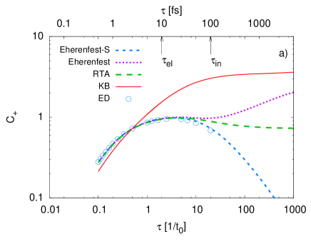
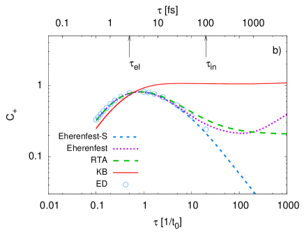
Figure 1: Average diffusivity $C_{+}(p)$ defined in Eq. (8) as a function of the timescale $\tau=p^{-1}$, at a temperature $T=0.2t_{0}=300K$. Panels (a) and (b) are respectively without $\Delta=0.0$ and with $\Delta=0.5t_{0}$ extrinsic disorder. The bold short-dashed curve (light blue) is obtained by solving the time-dependent Schrödinger equation on a $1024$-sites chain (Ehrenfest-S). The dotted curve (magenta) is the result of the dynamical Ehrenfest approach with vibrational frequency $\omega_{0}=0.05t_{0}$. The long-dashed line (green) is the RTA approximation with $\tau_{in}=\omega^{-1}_{0}$. The full (red) line is the result of the semiclassical Kubo bubble approximation Eq. (10). Open circles are results from exact diagonalization of a $256$-sites chain. The arrows mark the elastic and inelastic scattering times (see text).

Fig. 1 illustrates the function $C_{+}(p)$ defined in Eqs. (6)-(8), as calculated from the different methods outlined at the end of the preceding Section. This quantity has the meaning of a diffusivity averaged up to a time $\tau=1/p$ and therefore provides direct information on the quantum dynamics of electrons as a function of time. We fix $\lambda=0.17$, which is representative for the intrinsic electron-vibration coupling in rubrenereconcile09 , and set the temperature to $T=0.2t_{0}=300K$. The numerical results for a single electron in a pure organic semiconductor ($\Delta=0$) and in the presence of extrinsic disorder ($\Delta=0.5t_{0}=65meV$) are reported in Figs. 1a and 1b respectively. This value of $\Delta$ is close to the one that was derived from the analysis of angle-resolved photoemission spectra (ARPES) in crystalline pentacene filmsHatch .

All the methods outlined above yield a ballistic time evolution in the short-time limit. It can be shown that the average diffusivity at short times obeys exactly $C_{+}=2\langle v^{2}\rangle/p=2\langle v^{2}\rangle\tau$, which is ruled by the average band velocity $\langle v^{2}\rangle$ (cf. Appendix B). The ballistic regime is followed by a flattening of the average difusivity due to the onset of scattering processes, occurring on a timescale which we identify with the elastic scattering time, $\tau_{el}$ LeeRMP . From Fig. 1 we estimate approximately $\tau_{el}\sim 10^{-14}s$ in the pure case ($\Delta=0$), and $\tau_{el}\sim 5\cdot 10^{-15}s$ in the disordered case ($\Delta=0.5t_{0}$).

In the long time limit, the different methods yield qualitatively different behaviors reflecting the fundamentally distinct treatments of the intermolecular dynamics. Let us focus on the intrinsic case first, Fig. 1a. In the parent system with static disorder, the electrons are localized (Ehrenfest-S and ED, respectively blue short-dashed curve and open circles). The existence of a finite localization length $L(\tau)=const$ as $\tau\to\infty$ implies through Eq. (8) that the average diffusivity bends down and tends to $C_{+}\propto 1/\tau$ at long times. Restoring the dynamical nature of the inter-molecular vibrations via the RTA causes a departure from the localized behavior on the scale of the inelastic scattering time $\tau_{in}$, so that a diffusive behavior ($C_{+}=const$) is reached at long times (green long-dashed curve). We note that within the RTA the diffusion coefficient at $\tau\to\infty$ is necessarily lower than the maximum attainable value, which is obtained when $\tau_{in}\simeq\tau_{el}$.

Finally, the Ehrenfest method (purple, dotted line) also captures the departure from localization occurring at $\tau\simeq\tau_{in}$. However, this method yields a spurious superdiffusive behavior at long timesRTA11 , which is testified by a marked upturn of the diffusivity. This drawback leads to an overestimate of the mobility, whose value can vary strongly depending on the chosen simulation time. For this reason, the mobilities obtained from Ehrenfest simulations Troisi06 ; TroisiAdv ; Wang ; RTA11 ; Ishii should be taken with some care.

The results reported in Fig. 1a, that have been obtained using microscopic parameters appropriate for pure rubrene (the organic semiconductor with the highest mobility reported to date), indicate that even in ideal samples without extrinsic disorder the elastic scattering time at room temperature is shorter than the typical inelastic scattering time, $\tau_{el}<\tau_{in}$. This situation results from the combination of the large mass of the molecular units, which leads to low vibrational frequencies and therefore to large values of $\tau_{in}$, together with the typically weak inter-molecular transfer rates and their strong sensitivity to inter-molecular motions, which lead to short values of $\tau_{el}$. It is therefore expected to be a general feature of all organic semiconductors, resulting in a transport mechanism that is fundamentally different from that of inorganic materials. Specifically, a ”transient” localization regime emerges at intermediate times, $\tau_{el}<\tau<\tau_{in}$, where the electrons tend to localize (the diffusivity bends down) before a constant diffusivity sets back in at $\tau\gtrsim\tau_{in}$ (green long-dashed curve in Fig. 1a). When such transient localization is realized, the diffusion coefficient at long times depends on the history of the system at this intermediate stage, being inversely proportional to the inelastic time $\tau_{in}$, cf. Eq. (26).

The existence of a transient localization phenomenon invalidates in principle semiclassical treatments of electron transport, which are instead successful in inorganic materials. To illustrate this point we show in Fig. 1a the average diffusivity $C^{+}$ obtained from the semiclassical Kubo bubble approximation (red full line). Because in this approximation the backscattering processes at the origin of localization are neglected, the system evolves continuously from a ballistic to a diffusive behavior. Semiclassical approaches are therefore inadequate to describe electron transport in organic semiconductors where $\tau_{el}<\tau_{in}$. On the other hand, the present RTA is able to recover the semiclassical picture in the opposite regime where $\tau_{in}<\tau_{el}$. As discussed at the beginning of this Section we have that $C^{+}_{loc}(p)=2\langle v^{2}\rangle/p$ at short times. Using the RTA Eq. (25) and Eq. (11) yields a diffusion coefficient $D=\langle v^{2}\rangle\tau_{in}$, which is formally analogous to the Bloch-Boltzmann result.

The situation in the presence of extrinsic static disorder is not qualitatively modified with respect to the pure case, as can be seen from Fig. 1b. In particular, the inelastic scattering time remains unchanged, because it is determined by the intrinsic timescale of the intermolecular vibrations. However, an increased amount of disorder shifts the onset of localization $\tau_{el}$ to shorter times. This enlarges the time interval where the transient localization phenomenon is effective, with a consequent reduction of the diffusion coefficient.

Finally, one can wonder if the transient localization scenario, which was demonstrated here in the one-dimensional case, is robust in more realistic descriptions of OSC. For materials with a sizable in-plane anisotropy, i.e. such that the inter-molecular transfer rates in the transverse direction are much smaller than in the longitudinal direction, $t_{\perp}\ll t_{0}$, the one-dimensional picture is expected to remain valid up to times $t\simeq\hbar/t_{\perp}$. This is the situation that applies to Rubrene, according to recent photoemission data.Machida Because the elastic scattering time is very short, of the order of $\hbar/t_{0}$ or less (see Fig. 1), we have $\hbar/t_{\perp}\gg\tau_{el}$ and nothing prevents the transient localization to occur in this case. Backscattering processes remain relevant also in isotropic two-dimensional materials. Although the timescale for two-dimensional weak localization is known to be longer than $\tau_{el}$, LeeRMP the present scenario should remain qualitatively correct also in that case due to the strong intrinsic disorder present in OSC.

V.2 Temperature dependence of the mobility

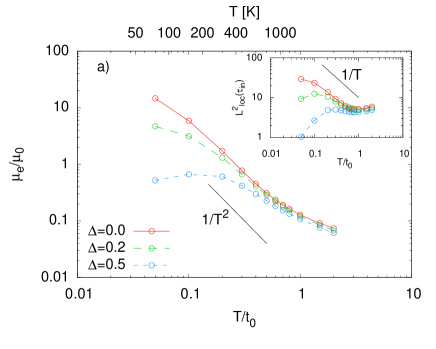
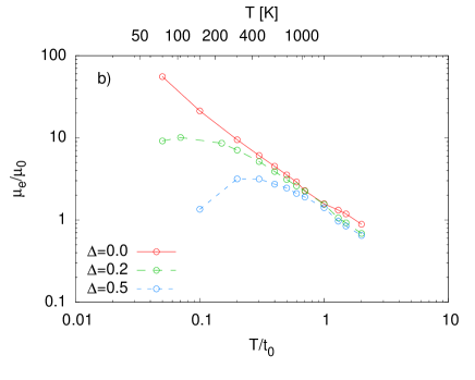
Figure 2: Mobility as a function of temperature calculated (a) within the RTA and (b) within the Kubo bubble approximation. The inset of panel (a) shows the behavior of the transient localization length $L^{2}_{loc}(\tau_{in})$ with $1/\tau_{in}=\omega_{0}=0.05t_{0}$. Mobilities are expressed in units of $\mu_{0}=ea^{2}/\hbar$, with $a$ the lattice spacing ($\mu_{0}=7cm^{2}/Vs$ taking $a=7.2\AA$ for rubrene). In this and all subsequent figures, we take $t_{0}$ as the unit of energy.

Fig. 2a shows the temperature dependence of the mobility as obtained from the RTA for different amounts of extrinsic disorder, $\Delta=0$, $0.2t_{0}$ and $0.5t_{0}$. The lowest accessible temperature is set by the limits of validity of our classical treatment for the molecular vibrations, namely $T\gtrsim\omega_{0}=0.05t_{0}$. The intrinsic mobility of pure compounds ($\Delta=0$, full red line) is a monotonically decreasing function of temperature, even though the microscopic transport mechanism is far from a conventional band transport, as discussed in Sec. V.1. Depending on the explored temperature window, a power law temperature dependence, $T^{-\gamma}$, can be identified. In practice the exponent $\gamma$ depends on how the transient localization length in Eq. (27) varies with temperature, due to the thermal increase of inter-molecular disorder.

The behavior of $L^{2}_{loc}(\tau_{in})$ is shown in the inset of Fig. 2a. In the temperature interval $T=200-600K$, the transient localization length decreases steadilyreconcile09 as $L^{2}_{loc}(\tau_{in})\propto a^{2}t_{0}/(\lambda T)$. Substituting this expression in Eq. (27) leads to a mobility $\mu_{e}\propto T^{-2}$  reconcile09 ; Troisi06 . Moreover, using explicitly the definition of $\lambda$ given in Sec. IV and the relation $1/\tau_{in}\sim\omega_{0}$ we obtain that the mobility in this regime increases with the third power of $\omega_{0}$, while it is independent of the transfer integral $t_{0}$. An analogous calculation in the semiclassical regime reconcile09 yields for the model under study a mobility proportional to $\omega_{0}$ and to $t_{0}^{1/2}$. In both cases, increasing $\omega_{0}$ results in an increase of the charge mobility, because it suppresses the effects of dynamical inter-molecular disorder. This observation suggests a possible strategy for the design of high mobility materials: rather than optimizing the inter-molecular $\pi$ overlaps that control the value of $t_{0}$, it could be advantageous to stiffen the inter-molecular vibrations either via an appropriate tayloring of the inter-molecular structure (e.g. by molecular functionalization) or via the interaction with a substrate (as in self-assembled monolayers).

The localization length becomes a weakly increasing function of T at very high temperatures, where a vibrationally assisted electron motion arises via the large fluctuations of the inter-molecular distances. This results in a weaker power law dependence of the mobility with exponent $\gamma<1$, which was termed “mobility saturation” in Ref. reconcile09 . Although such high temperatures are not attainable experimentally in rubrene, the mobility saturation regime could actually be observed in materials with a stronger electron-vibration coupling constant $\lambda$ than that considered here.

The inclusion of extrinsic disorder ($\Delta\neq 0$) causes a downturn of the mobility at low temperatures, that is reminiscent of a thermally activated behavior, i.e. $\mu_{e}$ increases with $T$. This behavior reflects a crossover between the extremely short $L^{2}_{loc}(\tau_{in})$ obtained at low temperatures and the larger intrinsic value at higher temperatures, as shown in the inset of Fig. 2a. note:transient The location of the crossover from extrinsic to intrinsic transport depends on the amount of extrinsic disorder, so that it can vary experimentally depending on the material and device quality. Correspondingly, a variety of behaviors ranging from thermal activation to a power law decrease can be realized in the experimental temperature window, which is possibly at the origin of the different temperature dependent mobilities observed in organic FETs.

The results of the semiclassical Kubo bubble approximation are shown in Fig. 2b for comparison. Despite the profound differences in the two descriptions of charge transport, the overall behavior obtained in the explored temperature interval is qualitatively similar. From a fundamental viewpoint, the fact that a thermally activated behavior is obtained for $\Delta\neq 0$ in both the RTA and the Kubo bubble approach indicates that the corresponding hopping processes (incoherent jumps from molecule to molecule) are already present at the semiclassical level, being captured by the Kubo bubble approximation in the strong disorder limit.Coehoorn This result means that the hopping behavior is not related to the quantum (backscattering) localization corrections, as the latter are not contained in the semiclassical treatment. As we proceed to show, the crossover from the intrinsic to the thermally activated regime can be explained in terms of the competition between highly conducting states located in the band range and weakly mobile states located in the band tails — a competition that is captured by both the RTA and the Kubo bubble approximation.

V.3 Energy resolved diffusivity and localization length

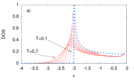
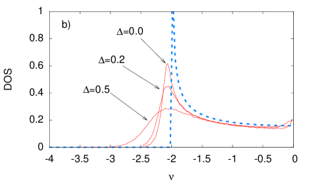
Figure 3: (a) Density of states in a pure crystal with intrinsic inter-molecular disorder and $\Delta=0$. The different curves correspond to increasing temperatures from $T=0.1t_{0}$ to $T=0.7t_{0}$. The dashed line is the DOS of the perfect crystal in the absence of thermal disorder ($\lambda=0$). (b) DOS at $T=0.2t_{0}$ for several values of the extrinsic disorder $\Delta$.

Based on Eq. (23), the electron mobility in a non-degenerate semiconductor arises from a weighted average of the energy-resolved diffusivity $D(\nu)$ via the thermal population of electronic states. The latter is measured by the thermally weighted DOS,

$$W(\nu)=\frac{\rho(\nu)e^{-\beta\nu}}{\int\rho(\nu)e^{-\beta\nu}},$$ (32)

which represents the normalized probability of occupation of the states at energy $\nu$. The functions $\rho(\nu)$, $D(\nu)$ and $W(\nu)$ are analyzed below.

Fig. 3 illustrates the evolution of the DOS $\rho(\nu)$ as a function of increasing thermal disorder in a pure sample (a) and upon increasing extrinsic disorder (b). The DOS of a perfectly ordered crystal is shown for reference (dashed). In both cases, the Van-Hove singularity marking the edge of the one-dimensional band at $\nu=-2t_{0}$ is rounded off and shifts deeper in energy, indicating an increase of the effective bandwidth. HoHu ; orgarpes11 ; Coropceanu12 In addition, tails are generated beyond the range of band states. Both the bandwidth increase and the extension of band tails are controlled by the amount of disorder. This can be quantified through the variance $s=\sqrt{8\lambda Tt_{0}}$ of the thermal fluctuations of the inter-molecular transfer intergrals in the intrinsic case reconcile09 (Fig.3a), and by the spread $\Delta$ of molecular energy levels in the extrinsic case HoHu (Fig.3b).

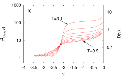
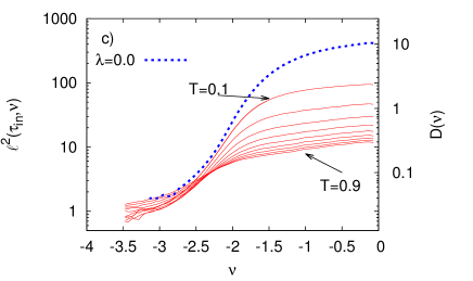
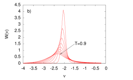
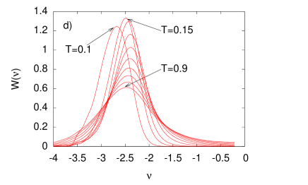
Figure 4: (a) Energy-resolved transient localization length squared $\ell^{2}(\tau_{in},\nu)$ (left axis) and diffusivity $D(\nu)$ (right axis) in a pure OSC, for increasing temperatures from $T=0.1t_{0}$ to $T=0.9t_{0}$. Parameters are the same as in the preceding figures. The length unit is the lattice spacing $a$. (b) Weighted DOS [see Eq. (32)] at the same temperatures. (c) and (d) show the same quantities in the presence of extrinsic disorder ($\Delta=0.5$). In panel (d) the temperature $T=0.15t_{0}$ has been added to highlight the crossover from extrinsic to intrinsic transport.

The diffusivity $D(\nu)$ obtained through the RTA in the pure case ($\Delta=0$) is shown in Fig. 4a (right axis scale). The diffusivity is directly related, through Eq. (29), to the square of the energy-resolved transient localization length, $\ell^{2}(\tau_{in},\nu)$, which is also shown on the same figure on the left axis. Analogous estimates for the localization length in the static disorder limit $\tau_{in}\to\infty$ can be found in Refs. reconcile09, ; Chang11, . The comparison with the DOS of Fig. 3a allows us to identify two distinct regions in the electronic spectrum, separated by a crossover region of width $\simeq s$ around the band edge. States located in the band region have a large diffusivity, that is strongly suppressed upon increasing the thermal disorder. Tail states induced by disorder below the band edge instead have a much lower diffusivity as a consequence of their more localized character. The diffusivity of tail states is essentially temperature independent and corresponds in our one-dimensional model to a minimum localization length of approximately one lattice spacing, $\ell(\tau_{in},\nu)\approx a$. We note that the existence of two distinct characteristic values of the localization length is in agreement with recent ESR measurements performed on pentacene transistors.Marumoto ; Matsui ; Mishchenko

The relative importance of band and tail states in the transport mechanism is determined by the weighting function $W(\nu)$, which is shown in Fig. 4b. At temperatures $T\lesssim 0.5t_{0}$, which includes the experimentally accessible range, the function $W(\nu)$ is peaked right in the crossover range that separates the band and tail states (cf. Fig. 3), with a sizable overlap on both sides. As expected for two conduction channels in parallel, the electronic transport in this case is dominated by the channel whose diffusivity is largest, i.e. the band states. Correspondingly, the temperature dependence of the mobility is governed by the suppression of the diffusivity in the band range, that is illustrated in Fig. 4a. Upon increasing the temperature, the weighting function progressively broadens and shifts towards the tail states. These eventually become the dominant transport channel, leading to the mobility saturation observed in Fig. 2a.

The energy-resolved diffusivity and transient localization length obtained in the presence of extrinsic disorder ($\Delta=0.5t_{0}$) are illustrated in Fig. 4c. The main difference with the pure case shown in Fig. 4a is that the crossover region separating tail and band states is now broadened by an amount $\propto\Delta$. Nevertheless, the typical values of the diffusivity both in the band region and in the tails remain close to their intrinsic values, provided that the temperature is not too low. This is more clearly seen in Fig. 5a, which shows the RTA diffusivity at increasing values of $\Delta$ for fixed $T=0.2t_{0}$. At lower temperatures ($T\leq 0.1t_{0}$) the extrinsic disorder eventually becomes dominant and the results tend to recover those obtained in the absence of intrinsic electron-vibration coupling ($\lambda=0$, dashed curve in Fig. 4c).

Since for $\Delta=0.5t_{0}$ the diffusivity is a monotonically decreasing function of $T$ for all states, the origin of the activated behavior of the mobility observed at low temperatures in Fig. 2a has to be sought elsewhere, i.e. in the weighting function $W(\nu)$. As illustrated in Fig. 4d, the behavior of $W(\nu)$ in the presence of extrinsic disorder is opposite to that of the pure case, Fig. 4b: at low temperature (here $T=0.1t_{0}$) the peak of the weighting function is located deep in the tail states and it moves towards the band upon increasing the temperature. Tail states with a low diffusivity therefore dominate the transport mechanism at low temperature, while the intrinsic regime is progressively recovered upon increasing the temperature. The crossover between these two regimes is signaled by a maximum in the mobility of Fig. 2a at a temperature that we denote $T^{*}$. By comparing the variances of intrinsic and extrinsic disorder given at the beginning of this Section, i.e. setting $s\simeq\Delta$, we obtain the following estimate for the crossover temperature: $T^{*}\simeq\Delta^{2}/(8\lambda t_{0})$. Taking $\Delta=0.5t_{0}$ and $\lambda=0.17$ gives $T^{*}=0.18t_{0}$, in good agreement with the data of Fig. 2a. The predicted crossover temperature for $\Delta=0.2t_{0}$ is $T^{*}=0.03t_{0}$, outside the studied range.

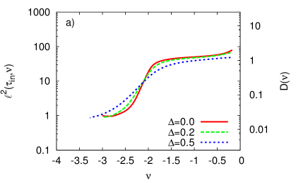
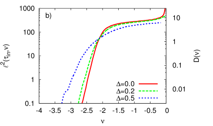
Figure 5: Energy resolved localization length squared $\ell^{2}(\tau_{in},\nu)$ within the RTA (a) and Kubo bubble approximations (b). In both cases we take $1/\tau_{in}=\omega_{0}=0.05t_{0}$

The Kubo bubble approximation yields qualitatively similar results for the temperature and $\Delta$ dependence of the diffusivity $D(\nu)$ (of course the DOS and weighting function $W(\nu)$ are exactly the same, as they are obtained in the common static limit). The main differences between the two methods are quantitative and arise from the inclusion or not of backscattering effects, i.e. they are indicative of the relevance of vertex corrections in the disordered system under study. As shown in Fig. 5, the diffusivity of band states in the Kubo bubble approximation is larger than in the RTA, corresponding to the fact that for band states the Kubo bubble essentially recovers the Boltzmann transport theoryreconcile09 where quantum localization phenomena are absent. This leads to larger values of the intrinsic mobility than in the RTA, as seen in Fig. 2b. Concerning tail states, the opposite is true. In the RTA the localization length and hence the diffusivity appear to be bound from below, which provides a lower bound to the mobility at low temperatures: taking $\ell(\tau_{in},\nu)>a$ from Fig. 5a yields $\mu_{e}>ea^{2}/(2\tau_{in}k_{B}T)$. This lower bound is absent in the Kubo bubble approximation, where $D(\nu)$ vanishes asymptotically for negative energies, being itself proportional to the DOS. It can actually be shown Coehoorn that a behavior of the form $\mu_{e}\propto e^{-(\Delta/2T)^{2}}$ is obtained from the Kubo bubble in the limit of strong disorder, $\Delta\gg t_{0}$. As a result the thermal activation at low temperatures is more pronounced in the Kubo bubble approximation than in the RTA. The two effects discussed here are at the origin of the much sharper crossover from extrinsic to intrinsic transport obtained in the Kubo bubble compared to the RTA, cf. Fig. 2.

VI Density dependence of the mobility

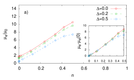
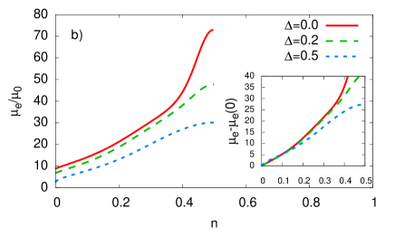
Figure 6: Mobility as a function of carrier concentration per molecule within (a) the RTA and (b) Kubo bubble approximation, for $T=0.2t_{0}$. The inset shows the variation of mobility with respect to its zero density limit.

The mobility obtained through Eq. (22) at finite electron concentration is shown in Fig. 6. The parameters are the same as in Fig. 1, i.e. $\lambda=0.17$, $T=0.2t_{0}=300K$. In both the RTA, Fig. 6a, and Kubo bubble approximation, Fig. 6b, we find a steady increase of the mobility with increasing density. This behavior can be understood as arising from a progressive filling of tail states, which occurs through a shift of the chemical potential towards the band region as the electron liquid becomes degenerate. This allows states with a higher diffusivity to be populated, via a shift of the the factor $-\partial f/\partial\nu$ in Eq. (22). This argument is only qualitatively correct however, because it neglects the fact that the diffusivity $D(\nu)$ itself depends on the density, which is instead correctly incuded in the results of Fig. 6. Based on the same argument, increasing the density of carriers will shift the crossover between the extrinsic and intrinsic regimes to lower temperatures. Such depinning effect can be achieved in OFETs through the application of a strong enough gate electric field.

We see from Fig. 6 that the curves describing the density dependence of the mobility for different degrees of extrinsic disorder are essentially parallel. The quantity $\mu_{e}-\mu_{e}(n=0)$, where the $n=0$ limiting value has been subtracted, is shown in the inset. Interestingly, it appears to be insensitive to the presence of extrinsic sources of disorder: the curves show a clear collapse for different values of the static disorder, that persists up to fairly large carrier concentrations. This indicates that at the considered temperature, $T=0.2t_{0}=300K$, the observed increase of mobility with density comes entirely from populating carriers with a strong band character (cf. Fig. 4). The quantity $\mu_{e}-\mu_{e}(n=0)$ could therefore be used to measure the mobility of band carriers even in samples with a sizable degree of disorder.

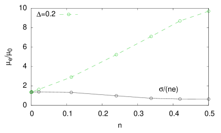
Figure 7: Mobility as a function of carrier concentration per molecule, obtained from the RTA for $T=0.2t_{0}$ and $\Delta=0.2t$ (dashed line, same as Fig. 6a). The full line is obtained by replacing the definition Eq. (15) by the expression $\mu_{e}=\sigma/(ne)$.

Finally, because large carrier concentrations are now customarily obtained in OFETs via liquid gating Frisbie ; Iwasa , the correct definition of the mobility, Eq. (15), should be used to analyze experiments, instead of the usual expression $\sigma/(ne)$ that only holds in the limit of vanishing density. To illustrate this point, we compare the results obtained with the two definitions in Fig. 7. Use of the low-density expression (black, full line) leads to an erroneous result, as it incorrectly predicts a reduction of the mobility upon increasing the density. To understand this result, we observe that for degenerate carriers, the susceptibility Eq. (20) is given by the DOS at the chemical potential, i.e. $\partial n/\partial\mu\simeq\rho(\mu)$. Using Eq. (15) we can then rewrite $\sigma/(ne)\simeq\mu_{e}k_{B}T\rho(\mu)/n$, which is itself proportional to the DOS (cf. Fig. 3b). In the present model an increase of the density implies a reduction of the DOS at the chemical potential, explaining the behavior observed in Fig. 7.

VII Conclusions

Based on a theoretical formalism that relates the Kubo formula for the conductivity to the time-resolved diffusivity of electronic states, we have analyzed the electronic transport mechanism in a model that accounts for several key ingredients relevant to organic semiconductors: the existence of narrow electronic bands, the dynamical disorder arising from the thermal vibrations of the molecules and the presence of extrinsic sources of disorder that are unavoidable in real samples and devices.

The presence of strong dynamical disorder is intrinsic to organic semiconductors and invalidates the usual semiclassical treatments of electronic transport that apply to inorganic semiconductors, calling for a theoretical approach that is able to treat quantum localization corrections in a controlled way. This is achieved here through a relaxation time approximation (RTA) that relates directly the carrier diffusivity to the localization properties of the electronic states. Within this theoretical scenario, the deviations from semiclassical transport are understood as arising from a transient localization of electrons, that takes place before the onset of a true diffusive behavior at long times. This phenomenon appears to be a characteristic feature of organic semiconductors, where the typical timescale of inter-molecular vibrations is longer than the elastic scattering time. The transient localization scenario is supported by numerical simulations on the time-dependent diffusivity RTA11 and by optical conductivity measurements in Rubrene OFETs Li ; Fischer .

Based on the present theory, the intrinsic transport mechanism in clean organic semiconductors is explained as the diffusive spread of localized wavefunctions rather than the scattering of delocalized waves by phonons and disorder. A power-law decay with temperature is predicted for the intrinsic mobility, which results from the reduction of the transient localization length as the thermal disorder increases. Our results suggest that the intrinsic mobility of organic semiconductors could be improved by tailoring crystal structures with stiffer inter-molecular bonds, as this would reduce the impact of thermal disorder on the charge transport.

The inclusion of extrinsic disorder causes a crossover from the intrinsic power-law behavior, persisting at high temperature, towards a thermally activated behavior induced by carrier trapping at low temperature. Increasing the electron concentration induces a depinning from trapped states, leading to an increase of the mobility and a progressive suppression of the thermally activated regime. Our results for the concentration dependence of the mobility generalize the findings obtained in the classical hopping limit $t_{0}\ll\Delta$ Bassler ; Coehoorn to the high mobility organic FETs of present interest, where the existence of electronic bands requires a quantum treatment of electron motion.

From a more general viewpoint, the present work demonstrates that the conductive properties of both pure and disordered organic semiconductors can be efficiently understood within a unified framework, by addressing the interplay between mobile states in the band region and strongly localized states in the band tails. The present results confirm and extend the considerations of Ref. reconcile09, by allowing for a proper inclusion of quantum localization phenomena. Interestingly, the relationship between the energy-resolved properties of electronic states and the resulting mobility, that we have exploited here, could also be generalized to study how the intrinsic polarizability of the organic crystals affects the transport characteristics, as was recently proposed in Ref. Minder, .

Appendix A Detailed balance and spectral representation

In this Appendix we set $e=1$ in addition to $\hbar=k_{B}=1$. By introducing the Laplace transform of the the retarded current-current correlation function $C_{+}(t)$

$$C_{+}(p)=\int_{0}^{\infty}dte^{-pt}C_{+}(t),$$ (33)

we can write the mean square displacement defined in Eq. (7) as

$$L^{2}(p)=\frac{C_{+}(p)}{p}.$$ (34)

Expressing $C_{+}(t)$ in terms of its Fourier transform $C_{+}(t)=\int\frac{d\omega}{2\pi}e^{-i\omega t}C_{+}(\omega)$ and using the reality of $C_{+}(t)$, which implies that $ReC_{+}(\omega)$ and $ImC_{+}(\omega)$ are respectively an even and an odd function of $\omega$, we have

$$C_{+}(p)=\int_{0}^{\infty}\frac{d\omega}{\pi}\frac{pReC_{+}(\omega)+\omega ImC_{+}(\omega)}{p^{2}+\omega^{2}}.$$ (35)

This equation can also be obtained using the analiticity of $C_{+}(\omega)$ in the complex upper half-plane with the help of Cauchy’s residue theorem for complex integration. The two terms in Eq. (35), respectively proportional to the real and imaginary part of $C^{+}$, bring the same contribution to the integral as can be checked via the Lehman representation of the correlation function

$$C_{+}(t)=\frac{1}{Z}\sum_{n,m}e^{-\beta E_{n}}|<n|J|m>|^{2}2\cos(\omega_{n,m}t),$$ (36)

where $|n>$ and $E_{n}$ are respectively the eigenvectors and eigenvalues of the Hamiltonian, that are supposed to be known, and $\omega_{n,m}=E_{n}-E_{m}$. The Fourier transform of Eq. (36) reads

$$ReC_{+}(\omega) = \frac{\pi}{Z}\sum_{n,m}e^{-\beta E_{n}}|<n|J|m>|^{2}\left[\delta(\omega-\omega_{n,m})+\delta(\omega+\omega_{n,m})\right]$$ (37)

$$ImC_{+}(\omega) = \frac{1}{Z}\sum_{n,m}e^{-\beta E_{n}}|<n|J|m>|^{2}\frac{2\omega}{\omega^{2}-\omega^{2}_{n,m}}$$ (38)

Using the result

$$P\int_{0}^{\infty}\frac{d\omega}{\pi}\frac{2\omega^{2}}{p^{2}+\omega^{2}}\frac{1}{\omega^{2}-\omega^{2}_{n,m}}=\frac{p}{p^{2}+\omega^{2}_{n,m}}$$ (39)

we arrive at

$$C_{+}(p)=\int_{0}^{\infty}\frac{d\omega}{\pi}\frac{2p}{p^{2}+\omega^{2}}ReC_{+}(\omega).$$ (40)

From this equation we can prove the limit used to obtain the Einstein’s relation Eq. (13), observing that as $p\rightarrow 0^{+}$ $\frac{1}{\pi}\frac{p}{p^{2}+\omega^{2}}\rightarrow\delta(\omega)$ then $\lim_{p\to 0}C_{+}(p)=\lim_{\omega\to 0}C_{+}(\omega)/2$.

Eqs. (3) and (8) are two relations which are not independent since the functions $C_{+}$ and $C_{-}$ are related by the detailed balance condition. The Fourier transforms of the retarded correlation functions $C_{\pm}(t)$ can be expressed as $C_{\pm}(\omega)=C_{>}(\omega)\pm C_{<}(\omega)$ where $C_{>}(\omega),C_{<}(\omega)$ are the Fourier transforms

$$C_{>}(\omega) = \int_{0}^{+\infty}dte^{i(\omega+i\delta)t}<\hat{J}(t)\hat{J}(0)>$$ (41)

$$C_{<}(\omega) = \int_{0}^{+\infty}dte^{i(\omega+i\delta)t}<\hat{J}(0)\hat{J}(t)>$$ (42)

and $\delta$ an infinitesimal positive quantity. The detailed balance condition reads Baym $ReC_{<}(\omega)=e^{-\beta\omega}ReC_{>}(\omega)$, which leads to

$$ReC_{-}(\omega)=\tanh\left(\frac{\beta\omega}{2}\right)ReC_{+}(\omega).$$ (43)

Applying the detailed balance Eq. (43) to Eq. (35) yields

$$C_{+}(p)=\int_{0}^{\infty}\frac{d\omega}{\pi}\frac{2p\;ReC_{-}(\omega)}{(p^{2}+\omega^{2})\tanh(\beta\omega/2)}$$ (44)

and using the Kubo formula Eq. (3) with the definition Eq. (34) we arrive at

$$L^{2}(p)=\int_{0}^{\infty}\frac{d\omega}{\pi}\frac{2\omega\sigma(\omega)}{(p^{2}+\omega^{2})\tanh(\beta\omega/2)}$$ (45)

which is Eq. (10) of the paper.

Similarly to Eq. (37), the Fourier transform of the anticommutator correlation function $C_{-}(\omega)$ can be expressed through its Lehman representation as

$$ReC_{-}(\omega)=\frac{\pi}{Z}\sum_{n,m}e^{-\beta E_{n}}|<n|J|m>|^{2}\left[\delta(\omega+\omega_{n,m})-\delta(\omega-\omega_{n,m})\right].$$ (46)

The two terms in the sum can be rearranged as

$$ReC_{-}(\omega)=\pi(1-e^{-\beta\omega})\frac{1}{Z}\left\{\sum_{n,m}e^{-\beta E_{n}}|<n|\hat{J}|m>|^{2}\delta(\omega+E_{n}-E_{m})\right\}.$$ (47)

We now consider single-particle Hamiltonians for which the number eigenstates $|\{n_{\alpha}\}>$ are such that $H|\{n_{\alpha}\}>=(\sum_{\beta}n_{\beta}\epsilon_{\beta})|\{n_{\alpha}\}>$. Once expressed using this basis Eq. (47) takes the form (in the grand canonical ensemble)

$$ReC_{-}(\omega)=\pi(1-e^{-\beta\omega})\frac{1}{Z}\left\{\sum_{\{n\}\{m\}}\Pi_{\alpha}e^{-\beta(\epsilon_{\alpha}-\mu)n_{\alpha}}|<\{n_{\alpha}\}|\hat{J}|\{m_{\alpha}\}>|^{2}\delta[\omega+\sum_{\alpha}\epsilon_{\alpha}(n_{\alpha}-m_{\alpha})]\right\}.$$ (48)

Since $\hat{J}$ is a single-particle operator, the individual eigenvalues obey $n_{\alpha}-m_{\alpha}=p_{\alpha}$ with $p_{\alpha}=-1,0,1$. Thus in the sum appearing in the $\delta$ function reduces to $\epsilon_{\alpha}-\epsilon_{\beta}$ where we have $p_{\gamma}=1$ when $\gamma=\alpha$, $p_{\gamma}=-1$ when $\gamma=\beta$ and $p_{\gamma}=0$ elsewhere. The matrix element of $\hat{J}$ reads in this case

$$|<\{n_{\alpha}\}|\hat{J}|\{m_{\alpha}\}>|^{2}=\sum_{\alpha,\beta}|<\alpha|\hat{J}|\beta>|^{2}n_{\alpha}(1-n_{\beta})$$ (49)

where $|\alpha>$ are single-particle states. The grand canonical averages appearing in Eq. (48) can be performed leading to

$$ReC_{-}(\omega)=\pi(1-e^{-\beta\omega})\sum_{\alpha,\beta}|<\alpha|\hat{J}|\beta>|^{2}<n_{\alpha}>(1-<n_{\beta}>)\delta(\omega+\epsilon_{\alpha}-\epsilon_{\beta}).$$ (50)

where we have made use of the vanishing of the diagonal elements of $\hat{J}$. We can introduce a dummy integration variable by writing

$$ReC_{-}(\omega)=\pi(1-e^{-\beta\omega})\int_{-\infty}^{\infty}d\nu f(\nu)[1-f(\omega+\nu)]\sum_{\alpha,\beta}|<\alpha|\hat{J}|\beta>|^{2}\delta(\omega+\nu-\epsilon_{\beta})\delta(\nu-\epsilon_{\alpha}).$$ (51)

where $f(\nu)$ is the Fermi function. Identifying the diagonal part of the spectral operator $\delta(\nu-\epsilon_{\alpha})=-\frac{1}{\pi}Im<\alpha|(\nu-\hat{H})^{-1}|\alpha>$ and taking into account that $(1-e^{-\beta\omega})f(\nu)(1-f(\omega+\nu))=f(\nu)-f(\omega+\nu)$ we finally arrive at

$$ReC_{-}(\omega)=\pi(1-e^{-\beta\omega})\int_{-\infty}^{\infty}d\nu f(\nu)(1-f(\omega+\nu))tr\left[\hat{\rho}(\nu)\hat{J}\hat{\rho}(\omega+\nu)\hat{J}\right].$$ (52)

Using Eq. (52) and Eq. (44) we obtain:

$$L^{2}(p)=\frac{2}{e^{2}}\int_{-\infty}^{\infty}d\nu\int_{0}^{\infty}d\omega\frac{1}{\omega^{2}+p^{2}}\frac{\left[f(\nu)-f(\omega+\nu)\right]}{\tanh(\beta\omega/2)}\ tr[\hat{\rho}(\nu)\hat{J}\hat{\rho}(\nu+\omega)\hat{J}]$$ (53)

Taking the low density limit, $\beta\mu\to-\infty$, we obtain

$$\frac{L^{2}(p)}{n}=\frac{2}{e^{2}Z}\int_{-\infty}^{\infty}d\nu e^{-\beta\nu}\int_{0}^{\infty}d\omega\frac{{1+e^{-\beta\omega}}}{\omega^{2}+p^{2}}\ tr[\hat{\rho}(\nu)\hat{J}\hat{\rho}(\nu+\omega)\hat{J}]$$ (54)

where the normalization factor is $Z={\int d\nu e^{-\beta\nu}\rho(\nu)}$.

Appendix B Optical conductivity sum-rules

Eq. (10) allows us to derive exact relationships between the asymptotic expansion of $C_{+}(p)$ [or equivalently $L^{2}(p)$] to certain integrals of the optical conductivity. Using the definition Eq. (34) we write Eq. (45) as

$$C_{+}(p)=\int_{0}^{\infty}\frac{d\omega}{\pi}\frac{2p\omega}{\omega^{2}+p^{2}}\frac{\sigma(\omega)}{\tanh(\beta\omega/2)}.$$ (55)

Taking the formal expansion in powers of $1/p$ we get

$$C_{+}(p)=\sum_{n=0}^{\infty}\frac{(-1)^{n}}{p^{2n+1}}S_{n}$$ (56)

where

$$S_{n}=\int_{0}^{\infty}\frac{d\omega}{\pi}\frac{2\omega^{2n+1}}{\tanh(\beta\omega/2)}{\sigma(\omega)}.$$ (57)

Taking into account the definition of the Laplace transform we obtain

$$C_{+}(p)=\sum_{n=0}^{\infty}\frac{2n+1}{p^{2n+1}}\frac{d^{n}C_{+}(t)}{dt^{n}}|_{t=0}.$$ (58)

The leading term of the asymptotic expansion ($n=0$) gives $C_{+}(p)\simeq C_{+}(t=0)/p$ where $C_{+}(t=0)=<J^{2}>$.

Equating the coefficients of the expansions we get

$$\frac{d^{n}C_{+}(t)}{dt^{n}}|_{t=0}=(-1)^{n}S_{n}$$ (59)

which reads for $n=0$

$$C_{+}(t=0)=\int_{0}^{\infty}\frac{d\omega}{\pi}\frac{2\omega}{\tanh(\beta\omega/2)}{\sigma(\omega)}.$$ (60)

Setting $p=1/\tau$ as in Fig. 1 we have that in the short time limit $C_{+}(\tau)=C_{+}(t=0)\tau=<J^{2}>\tau$. While the RTA obeys this sum rule because the correlation function $C^{+}$ is exact at short times, the Kubo bubble approximation does not, which results in the slight discrepancy observed in Fig. 1 in the ballistic regime. This can be related via Eq. (B6) to the different behaviour obtained for $\sigma(\omega)$ in the two approximations and points to the relevance of vertex corrections at all frequencies.

Appendix C Boltzmann theory from the RTA

The quantity $\ell(p,\nu)^{2}$ is evaluated in practice from

$$\ell^{2}(p,\nu)=\frac{2}{\rho(\nu)}\int_{0}^{\infty}\frac{d\omega}{p^{2}+\omega^{2}}\frac{1-e^{-\beta\omega}}{\tanh(\beta\omega/2)}tr[\hat{\rho}(\nu)\hat{J}\hat{\rho}(\nu+\omega)\hat{J}]$$ (61)

or, equivalently,

$$\ell^{2}(p,\nu)=\frac{2}{\rho(\nu)}\int_{-\infty}^{\infty}d\omega\frac{1}{p^{2}+\omega^{2}}tr[\hat{\rho}(\nu)\hat{J}\hat{\rho}(\nu+\omega)\hat{J}].$$ (62)

These relations are obtained from the definition Eq. (54) via Eq. (28).

The Bloch-Boltzmann theory is customarily obtained from the RTA by taking the noninteracting band eigenstates as the reference system. Within the present formalism this amounts to evaluating the trace in the above equation assuming that the eigenstates of the Hamiltonian are good momentum eigenstates, $|k\rangle$, with energy $E_{k}$. In that case $\langle k|\hat{J}|k\rangle=v_{k}=dE_{k}/dk$ and we obtain

$$\ell^{2}(p,\nu)=\frac{2}{\rho(E_{k})}\sum_{k}\frac{v_{k}^{2}}{p^{2}}\delta(\nu-E_{k})$$ (63)

Using Eqs. (23) and (29), with $\tau=1/p$ the relaxation time for momentum eigenstates yields the Boltzmann form of the mobility:

$$\mu=\frac{e}{k_{B}T}\langle\tau v_{k}^{2}\rangle$$ (64)

where the thermal average is defined as $\langle\tau v_{k}^{2}\rangle=\frac{\sum_{k}e^{-\beta E_{k}}\tau v_{k}^{2}}{\sum_{k}e^{-\beta E_{k}}}$.

References

- (1) V. Podzorov, E. Menard, J. A. Rogers, M. E. Gershenson, Phys. Rev. Lett. 95, 226601 (2005).
- (2) H. Xie, H. Alves, A. F. Morpurgo, Phys. Rev. B 80, 245305 (2009).
- (3) T.Sakanoue and H.Sirringhaus, Nat.Mater. 9, 736 (2010).
- (4) C. Liu, T. Minari, X. Lu, A. Kumatani, K. Takimiya, and K. Tsukagoshi, Adv. Mater. 23, 523 (2011).
- (5) N. A. Minder, S. Ono, Z. Chen, A. Facchetti, and A.F. Morpurgo, Adv. Mater. 24, 503 (2012).
- (6) L. Friedman, Phys. Rev. 140, A1649 (1965).
- (7) Y. C. Cheng et al., J. Chem. Phys. 118, 3764 (2003).
- (8) S. Ciuchi and S. Fratini, Phys. Rev. Lett. 106, 166403 (2011).
- (9) N. Vukmirović, C. Bruder and V. M. Stojanović, Phys. Rev. Lett. 109, 126407 (2012)
- (10) R. W. Munn and R. J. Silbey, J. Chem. Phys. 83, 1854 (1985).
- (11) A. Troisi & G. Orlandi, Phys. Rev. Lett. 96, 086601 (2006).
- (12) J.-D. Picon, M. N. Bussac, and L. Zuppiroli, Phys. Rev. B 75, 235106 (2007).
- (13) S. Fratini and S. Ciuchi, Phys. Rev. Lett. 103, 266601 (2009).
- (14) S. Ciuchi, S. Fratini and D. Mayou, Phys. Rev. B 83, 081202(R) (2011).
- (15) N. Karl, Organic Electronic Materials, edited by R. Farchioni and G. Grosso (Springer-Verlag, Berlin, 2001), pp. 283-326.
- (16) M. Fischer, M. Dressel, B. Gompf, A.K. Tripathi,and J. Pflaum, Appl. Phys. Lett. 89, 182103 (2006).
- (17) Z. Q. Li, V. Podzorov, N. Sai, M. C. Martin, M. E. Gershenson, M. DiVentra, and D. N. Basov, Phys. Rev. Lett. 99, 016403 (2007).
- (18) I. N. Hulea, S. Fratini, H. Xie, C. L. Mulder, N. N. Iossad, G. Rastelli, S. Ciuchi, A. F. Morpurgo, Nat. Mater. , 5, 982 (2006).
- (19) T. Richards, M. Bird, H. Sirringhaus, J. Chem. Phys. 128, 234905 (2008).
- (20) W.L. Kalb, S. Haas, C. Krellner, T. Mathis, and B. Batlogg, Phys. Rev. B 81, 155315 (2010).
- (21) J.-F. Chang, T. Sakanoue, Y. Olivier, T. Uemura, M.-B. Dufourg-Madec, S. G. Yeates, J. Cornil, J. Takeya, A. Troisi and H. Sirringhaus, Phys. Rev. Lett. 107, 066601 (2011)
- (22) D. Mayou, Phys. Rev. Lett. 85, 1290 (2000).
- (23) G. Trambly de Laissardière, J.-P. Julien, and D. Mayou, Phys. Rev. Lett. 97, 026601 (2006).
- (24) G. Trambly de Laissardière and D. Mayou, Mod. Phys. Lett. 25, 1019 (2011).
- (25) G. D. Mahan “Many particle physics”, second edition, Plenum Press N.Y. and London (1990).
- (26) We are using the same symbols for the Fourier and Laplace transforms for simplicity. These are however different functions and are implicitly specified by their argument, or respectively.
- (27) R. Kubo, J. Phys. Soc. Japan. 12, 570 (1957).
- (28) Y. Li, Y. Yi, V. Coropceanu and J.-L. Brédas, Phys., Rev. B 85, 245201 (2012).
- (29) S. Ciuchi, R. C. Hatch, H. Höchst, C. Faber, X. Blase, and S. Fratini, Phys. Rev. Lett. 108, 256401 (2012)
- (30) P. A. Lee and T. V. Ramakrishnan, Rev. Mod. Phys. 57, 287 (1985).
- (31) The full neglect of vertex corrections also amounts to setting the transport scattering time equal to the quasiparticle lifetime Mahan . In the band limit, this leads to an overestimate of the mobility by at most a factor of two. The multiplicative factor approaches one in the case where the transport is dominated by incoherent tail states.
- (32) S. Fratini and S. Ciuchi, Phys. Rev. Lett. 91, 256403 (2003).
- (33) H. Bässler, Phys. Status Solidi B 175, 15 (1993).
- (34) R. Coehoorn, W. F. Pasveer, P. A. Bobbert, and M. A. J. Michels, Phys. Rev. B 72, 155206 (2005).
- (35) D. J. Thouless, Phys. Rev. Lett. 39, 1167 (1977).
- (36) V. Cataudella, G. De Filippis, and C. A. Perroni, Phys. Rev. B 83, 165203 (2011).
- (37) A. Troisi, Adv. Mat. 19, 2000 (2007).
- (38) K. Hannewald & P. A. Bobbert. Phys. Rev. B 69, 075212 (2004).
- (39) L. J. Wang, Q. Peng, Q. K. Li, and Z. Shuai. J. Chem. Phys. 127, 044506 (2007).
- (40) L. Wang, D. Beljonne, L. Chen and Q. Shi, J. Chem. Phys. 134, 244116 (2011).
- (41) H. Ishii, K Honma, N. Kobayashi and K. Hirose, Phys. Rev. B 85, 245206 (2012).
- (42) S. Fratini and S. Ciuchi, Phys. Rev. B 72, 235107 (2005).
- (43) S. Machida, et al., Phys. Rev. Lett. 104, 156401 (2010).
- (44) The transient localization length is predicted to saturate to a constant value at very low temperatures, because is necessarily finite at any finite value of as [see Eq. (10)]. This implies a dependence at low temperature. This behavior however occurs beyond the limits of validity of our classical treatment for the molecular vibrations, so that it is not shown in Fig. 2.
- (45) K. Marumoto, S. I. Kuroda, T. Takenobu, and Y. Iwasa Phys. Rev. Lett. 97, 256603 (2006).
- (46) H. Matsui, A. S. Mishchenko, and T. Hasegawa, Phys. Rev. Lett. 104, 056602 (2010).
- (47) A. S. Mishchenko, H. Matsui and T. Hasegawa, Phys. Rev. B, 85, 085211 (2012).
- (48) G. Baym and L. P. Kadanoff, ”Quantum statistical mechanics: Green’s function methods in equilibrium and nonequilibrium problems” W. A: Benjamin, N.Y. (1962).
- (49) The Thouless Thouless definition adopted in Ref. reconcile09, for the localization length differs in principle from the definition Eq. (28) for two reasons. First, the localization length reported in Ref. reconcile09, was weighted by the density of states at energy . Second, the present represents the dynamical localization of electronic states on a timescale , while the Thouless length is defined in the static limit .
- (50) M. J. Panzer and C. D. Frisbie, Appl. Phys. Lett. 88, 203504 (2006)
- (51) H. Shimotani, H. Asanuma, J. Takeya and Y. Iwasa, Appl. Phys. Lett 89, 203501 (2006)