Engineering light localization in a fractal waveguide network

Abstract

We present an exact analytical method of engineering the localization of electromagnetic waves in a fractal waveguide network. It is shown that, a countable infinity of localized electromagnetic modes with a multitude of localization lengths can exist in a Vicsek fractal geometry built with diamond shaped monomode waveguides as the ‘unit cells’. The family of localized modes form clusters of increasing size. The length scale at which the onset of localization for each mode takes place can be engineered at will, following a well defined prescription developed within the framework of a real space renormalization group. The scheme leads to an exact evaluation of the wave vector for every such localized state, a task that is non-trivial, if not impossible for any random or deterministically disordered waveguide network.

I Introduction

Since its inception, the phenomenon of Anderson localization in a disordered lattice pwa1 has been found to be ubiquitous in diverse fields of condensed matter physics and materials science. While the popular domain of interest is related to electronic systems, where the quantum interference plays a pivotal role in localizing electronic eigenstates in presence of disorder angus ; thouless ; schreiber ; alberto1 ; alberto2 ; zilly , the effect is by no means, confined to electrons, and extend over a variety of phenomena ranging from spin freezing in one dimensional semiconductors echeverria , localization in optical lattices sankar1 ; edwards ; roati , or the localization of matter waves (cold atoms forming Bose-Einstein condensates) gavish ; lye , to name a few. Incidentally, the latter has recently been observed experimentally in one dimensional matter waveguides, where the random potential is generated by laser speckles billy .

In 1984 Sajeev John pointed out that the idea of localization goes far beyond the electronic systems, and is actually a general phenomenon common to any wave propagation in systems with disorder john . Anderson followed with a seminal paper considering the idea of localization of classical waves, in an attempt to work out the theory of white paints pwa2 . The field gathered momentum in the last couple of decades and a considerable volume of literature related to the localization of classical waves, particularly light, ultrasound and microwave is now in existence jovic1 ; bliokh ; jovic2 ; sutherland ; asatryan ; hodges ; he ; yablonovich1 ; shi .

The study of localization of light in disordered media has been patronized by the discovery of the photonic band gap (PBG) materials soukoulis ; john2 ; yablonovitch2 . These systems exhibit gaps in the frequency spectrum in which propagation of electromagnetic waves is forbidden. This has important implications in both fundamental science and technological applications.

Photonic gaps, apart from materials with a large dielectric constant, can also be observed in waveguide networks, as proposed by several groups over the past years zhang ; dobrzynski ; vasseur ; pradhan ; li ; sheelan1 ; sheelan2 ; lu1 ; lu2 . Anderson localized eigenmodes are observed inside the photonic gaps and excellent agreement between theory and experiments has been obtained zhang . The network models are able to localize a propagating wave by virtue of the geometrical arrangement of the waveguide segments. Of particular interest are a wide variety of models based on waveguide networks designed following a deterministic fractal geometry li ; sheelan1 ; sheelan2 ; lu1 ; lu2 , where the gaps result from the typical topology exhibited the hierarchical arrangement of the waveguide segments. The present communication also deals with a hierarchically designed (fractal geometry) waveguide network, but addresses a deeper fundamental question regarding wave localization in such systems, as explained below.

Fractals or hierarchical geometries in general cause an excitation to localize kadanoff ; rammal ; kappertz ; schwalm1 . The energy spectrum turns out to be singular continuous kadanoff , with a gap in the vicinity of every energy. Nevertheless, there can be a countable infinity of extended eigenfunctions with high (or even, perfect) transmittivity, even though there is no translational order in such systems. Once again, this is true for electrons bibhas ; anirban ; xiang ; arun1 ; macia ; moritz ; arun2 , and classical waves as well sheelan1 ; sheelan2 . A curious point, apparently gone unnoticed or un-appreciated so far is that, while a precise determination of the eigenvalues corresponding to the extended eigenmodes is possible in the above cases of hierarchically grown fractal networks, the task seems to be practically impossible when it comes to an exact evaluation of eigenvalues of the localized modes in such hierarchical systems in their thermodynamic limits. Direct diagonalization of the Hamiltonian (in the electronic case), or an exact numerical solution of the wave equation doesn’t help, as the overall character of the spectrum in all the cases is highly fragmented, and the eigenvalues obtained from a finite sized network are likely to slip away from the spectrum once we go over to a higher generation. This problem has recently been addressed in the context of electron localization in fractal space biplab , and we carry forward the central idea floated in Ref. biplab to evaluate the exact wavelengths (wave vectors) of electromagnetic waves that can be localized at will in a properly designed hierarchical single channel network. To the best of our knowledge, this issue remains unaddressed so far in the literature in the context of localization of wave, light in particular.

We design a Vicsek fractal network vicsek consisting of diamond shaped loops each arm of which mimics a single mode linear waveguide [see Fig. 1]. While examination of the localized mode eigenvalues and the nature of localization are indeed the major factors motivating this work, other interests in such a study are related to the general spectral character and classical wave transport in these systems.

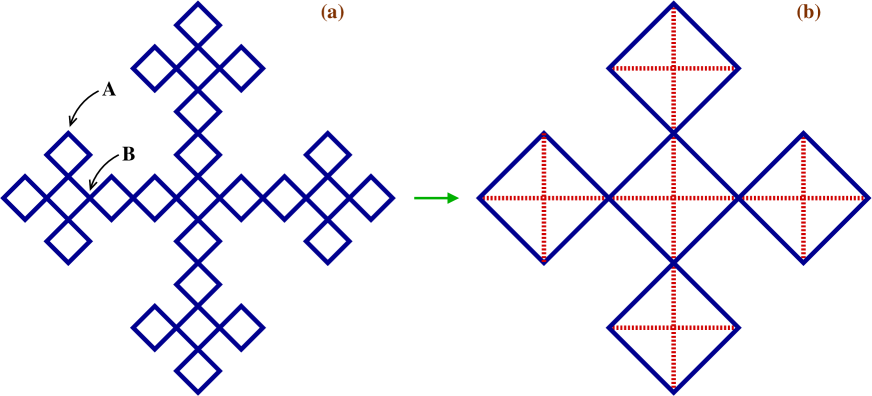
Figure 1: (Color online) (a) Schematic view of the second generation of an infinite diamond-Vicsek waveguide network. The vertices at the junction of two waveguides are named as ‘$A$’ in the text, while those in the bulk (at the crossing of four waveguides) are termed ‘$B$’. (b) Renormalized version of (a) with the dotted lines indicating the diagonal ‘hopping’ which is generated due to renormalization.

As one can easily appreciate, the geometry of a diamond-Vicsek network provides an interesting culmination of the ‘open’ character of a typical Vicsek pattern and closed loops at shorter scales of length. This is in marked contrast to the much studied Sierpinski gasket waveguide network li , which is a closed structure, or to the other deterministic waveguide networks sheelan2 ; lu1 . The presence of the loops generates a possibility of an effectively long ranged propagation of waves between the various vertices, and its effect on the localization or de- localization of waves is worth studying.

We find interesting results. For an infinite hierarchical geometry, such as presented above, a countable infinity of eigenmodes with a multitude of localization lengths can be precisely detected. One can work out an exact mathematical prescription to specify the length scale at which the onset of localization begins. The localization can in principle, be delayed (staggered) in position space and the corresponding wave vectors (or, wavelengths) can be exactly evaluated following the same prescription based on a real space renormalization group (RSRG) method southern . In addition, it is shown that for a given set of parameters, the center of the spectrum corresponds to a perfectly extended eigenmode, with the parameters describing the system exhibiting a fixed point behavior. This central extended mode is flanked on either side by localized wave functions with a hierarchy of localization lengths.

In what follows we describe the results. In Sec. II, the model and the mathematical method of handling the problem are presented. Section III discusses the results and their analyses, and in Sec. IV we draw our conclusions .

II The model and the method

II.1 The wave equation and its discretization

We have considered a waveguide network formed by waveguide segments having the same lengths arranged in a Vicsek fractal geometry vicsek . Each segment has a single channel for wave propagation. The wave function $\psi_{ij}$ between any two nodal points $i$ and $j$ satisfies the wave equation:

$$\frac{\partial^{2}\psi_{ij}(x)}{\partial x^{2}}+\frac{\omega^{2}}{c^{2}}\psi_{ij}(x)=0$$ (1)

where $\omega$ is the frequency of the wave, $c$ is the speed of wave propagation and $x$ is the distance measured from the $i$th node. The above equation has the solution of the form alexander ; ping

$$\psi_{ij}(x)=\psi_{i}\frac{\sin[k(\ell_{ij}-x)]}{\sin(k\ell_{ij})}+\psi_{j}\frac{\sin(kx)}{\sin(k\ell_{ij})}$$ (2)

where $k=\omega/c$, $\ell_{ij}$ is the length of the segment between the node $i$ and $j$, and $\psi_{i}$ and $\psi_{j}$ are the values of the wave function at the $i$th and $j$th nodes respectively. The flux conservation condition:

$$\sum_{j}\left[\frac{\partial}{\partial x}\psi_{ij}(x)\right]_{x=0}=0$$ (3)

where the summation $j$ is over all the nodes linked directly to $i$, leads to a discretized version of Eq. (1) ping , viz.,

$$-\psi_{i}\sum_{j}\cot\theta_{ij}+\sum_{j}\psi_{j}/\sin\theta_{ij}=0$$ (4)

where $\theta_{ij}=k\ell_{ij}=ka$, $a$ being the constant length of a waveguide, as considered in all the calculations which follow. Eq. (4) resembles a tight binding difference equation depicting the propagation of non-interacting electrons in a lattice, viz.,

$$(E-\epsilon_{i})\psi_{i}=\sum_{j}t_{ij}\psi_{j}$$ (5)

with the ‘electron energy’ $E$ can be put equal to $2\cos ka$, the ‘on-site potential’ $\epsilon_{i}=2\cos ka+\sum\limits_{j}\cot\theta_{ij}$ and ‘hopping matrix element’ $t_{ij}=1/\sin\theta_{ij}$. It should be appreciated that the choice of $E=2\cos ka$ is completely arbitrary, and this does not affect the final results in any way. As seen in Fig. 1, the Vicsek waveguide network has two types of nodal points, viz., type $A$ (having two neighboring nodal points) and type $B$ (having four neighboring nodal points). Accordingly, the equivalent ‘on-site potentials’ are assigned two values, viz., $\epsilon_{A}=2\cos ka+2\cot ka$ and $\epsilon_{B}=2\cos ka+4\cot ka$ respectively. The ‘overlap integral’ along an arm of the waveguide is $t=1/\sin ka$. There is no second neighbor tunneling of the wave to begin with. But it will grow with RSRG.

We now proceed to describe the physics of wave propagation in such a fractal geometry by exploiting this exact analogy with the corresponding electronic problem.

II.2 The RSRG scheme

A renormalized version of the fractal network is easily obtained by decimating a subset of vertices from the original geometry. This implies one has to eliminate a subset of the wave amplitudes from the difference equations (5) in terms of the surviving vertices [see Fig. 1(b)]. This results in the following set of recursion relations for the system parameters.

$$\epsilon_{A}^{\prime} = \epsilon_{A}+\left[\frac{2t^{2}}{E-\epsilon_{A}-\lambda}+\frac{\left(\lambda+\dfrac{2t^{2}}{E-\epsilon_{A}-\lambda}\right)^{2}\left\{(E-\epsilon_{B})-\dfrac{2t^{2}}{E-\epsilon_{A}-\lambda}-\xi\right\}}{\left\{(E-\epsilon_{B})-\dfrac{2t^{2}}{E-\epsilon_{A}-\lambda}-\xi\right\}^{2}-\left(\lambda+\xi\right)^{2}}\right],$$

$$\epsilon_{B}^{\prime} = \epsilon_{B}+2\left[\frac{2t^{2}}{E-\epsilon_{A}-\lambda}+\frac{\left(\lambda+\dfrac{2t^{2}}{E-\epsilon_{A}-\lambda}\right)^{2}\left\{(E-\epsilon_{B})-\dfrac{2t^{2}}{E-\epsilon_{A}-\lambda}-\xi\right\}}{\left\{(E-\epsilon_{B})-\dfrac{2t^{2}}{E-\epsilon_{A}-\lambda}-\xi\right\}^{2}-\left(\lambda+\xi\right)^{2}}\right],$$

$$t^{\prime} = \frac{t\left\{\lambda(E-\epsilon_{A}-\lambda)+2t^{2}\right\}^{2}}{\left\{E^{2}-(\epsilon_{A}+\epsilon_{B})(E-\lambda)-2E\lambda+\lambda^{2}-2t^{2}+\epsilon_{A}\epsilon_{B}\right\}^{2}-4t^{2}(E-\epsilon_{A}-\lambda)^{2}},$$

$$\lambda^{\prime} = \frac{\left(\lambda+\dfrac{2t^{2}}{E-\epsilon_{A}-\lambda}\right)^{2}\left(\lambda+\xi\right)}{\left\{(E-\epsilon_{B})-\dfrac{2t^{2}}{E-\epsilon_{A}-\lambda}-\xi\right\}^{2}-\left(\lambda+\xi\right)^{2}}.$$ (6)

where $\xi=2t^{2}(E-\epsilon_{A}-\lambda)/\Delta$ with $\Delta=(E-\epsilon_{A}-\lambda)(E-\epsilon_{B}-\lambda)-2t^{2}$, and $\lambda=0$ at the beginning.

The scaling generates an effective second neighbor ‘hopping’ (overlap) $\lambda^{\prime}$, as is obvious from the above set of recursion relations and the diagram 1(b). It is important to appreciate that, the growth of a $\lambda^{\prime}$, unlike the electronic case biplab , does not have any physical significance here, as there is no real ‘overlap’ of the wave amplitudes. The light is essentially confined within the waveguide.

These recursion relations will now be used to obtain information about the local density of eigenmodes at specific sites of the system, and the localized or extended character of the modes, as discussed below.

III Results and discussion

III.1 Local density of eigenmodes

As already stated, the exact mapping of the wave equation on to a discrete Schrödinger type equation allows us to extract information about the density of electromagnetic modes through a Green’s function analysis southern . We present in Fig. 2 the density of modes at a $B$-vertex, which is given by,

$$\rho^{(B)}(ka)=\lim_{\eta\rightarrow 0}\,\left[-\dfrac{1}{\pi}\,\text{Im}\,\{G^{(B)}(ka+i\eta)\}\right]$$ (7)

The distribution of eigenmodes, plotted within $ka<0<2\pi$, shows clusters of non-zero values over a finite range of the wave vector $k$, and is found to be symmetric around $ka=\pi/2$. The fragmented Cantor-like character, typical signature of a fractal spectrum, is apparent. An idea about the character of the eigenmodes can be obtained by observing the flow of $t$ under successive RSRG iterations. In general, for an arbitrary value of $ka$, for which the density of modes is non-zero, $t^{(n)}\rightarrow 0$ as the number of iterations $n$ increases, implying a localized character of the corresponding eigenmode southern ; bibhas . However, for $ka=(2m+1)\pi/2$, both the first and the second neighbor ‘hopping integrals’ $t$ and $\lambda$ remain non-zero for an indefinite number of iterations. In fact, we observe a one cycle fixed point of the entire parameter space, viz., $\{\epsilon_{A}^{\prime},\epsilon_{B}^{\prime},t^{\prime},\lambda^{\prime}\}=\{\epsilon_{A},\epsilon_{B},t,\lambda\}$. The fact that $t$ and $\lambda$ remain finite at all stages of RSRG implies that there is a non-zero overlap between the wave amplitudes at all scales of length, and the corresponding mode is an extended one.

The neighborhood of $ka=(2m+1)\pi/2$ has been scanned minutely. The self similarity of the spectrum is always seen with dense patches of eigenvalues clustered throughout the intervals. For many of these eigenvalues $t$ and $\lambda$ remain finite under successive decimation for a large number of steps. This indicates that every local band center at $ka=(2m+1)\pi/2$ is flanked either by extended modes or at least, eigenmodes with very large localization lengths.

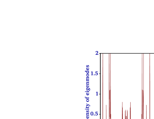
Figure 2: (Color online) Local density of eigenmodes at a bulk $B$-type vertex of an infinite diamond-Vicsek waveguide network.

III.2 Explicit construction of localized modes

The deterministic Vicsek fractal waveguide is self-similar at all scales of length. This feature allows us to explicitly construct a special distribution of wave functions by suitably exploiting the difference equations Eq. (5). These ‘special’ eigenmodes are localized and extend over clusters of single channel waveguide segments of various sizes. The planar extent of such clusters depends on the eigenvalue corresponding to the localized mode, and can be small or enormous, depending on the wavelength (or, wave vector). The construction is similar to our recent work biplab on electronic states.

To elaborate, let us set

$$E=\epsilon_{B}(n)-2\lambda(n)$$ (8)

where, $n$ refers to the stage of renormalization. This is in general, a polynomial equation in $E$ (and hence, in $k$). The zeros of this equation will be the allowed wave vectors for the infinite system if, and only if, with them, one can satisfy Eq. (5) locally at every vertex of the network. This task can be accomplished by trying to draw a non- trivial distribution of amplitudes for a value of $E$ ($ka$) obtained from Eq. (8) on the undecimated vertices of an $n$-step renormalized network, and then trying to figure out the amplitude distribution on the original waveguide structure at the bare length scale. This can indeed be done, as we demonstrate in Fig. 3(a) for $n=1$.

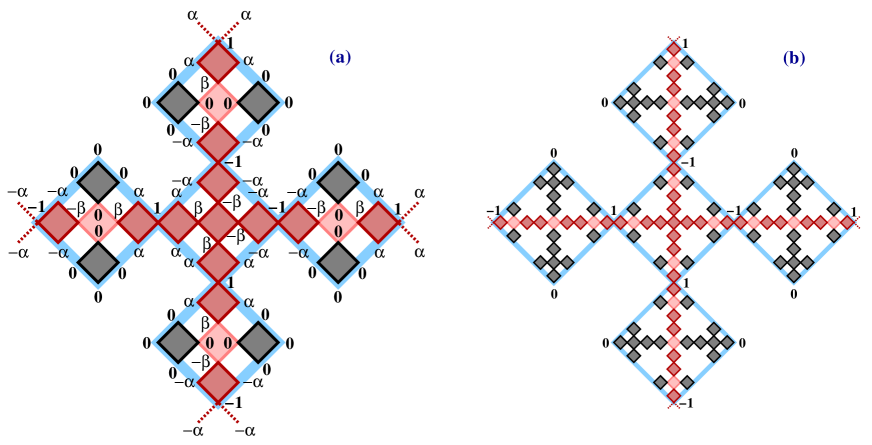
Figure 3: (Color online) (a) Distribution of amplitudes of the wave function for $ka=\pi/6$ (obtained by solving Eq. (8) for $n=1$) on a second generation network. The dark shaded plaquettes with black lines at the boundary embrace network vertices with zero amplitude. The deep red waveguide segments (covering a dark red shaded region) connect vertices with non-zero amplitude, and ‘glow’ with maximum intensity. The lighter red lines represent waveguide segments which have an intermediate intensity profile. The amplitudes of the wave are marked by the numbers $\pm 1$, $0$, $\pm\alpha$ and $\pm\beta$ respectively, where $\alpha=-\sqrt{3}/2$ and $\beta=1/2$. (b) The distribution of wave amplitudes for $ka=\pi/6$ on a third generation network. The thick blue highlighted lines represent one- and two-step renormalized lattices in (a) and (b) respectively.

For $n=1$ Eq. (8) reduces to

$$\cos ka(2\cos 2ka-1)=0$$ (9)

Roots of the above equation are $ka=\pm\pi/2$ and $ka=\pm\pi/6$. $ka=\pi/2$ (or, equivalently, $-\pi/2$) is of course, the extended mode. The root $ka=\pi/6$ leads to the construction of wave amplitudes as shown in Fig. 3. It is not difficult to extend the construction depicted in Fig. 3(a) even to a network of an arbitrarily large size, where the end vertices are not actually visible. We are still able to satisfy Eq. (5) locally at every vertex while drawing this distribution and thus, $k=\pi/6a$ definitely belongs to the spectrum of the infinite system, a fact that has been cross-checked by evaluation the LDOS at the $A$- and the $B$-sites at this special value of $k$. We get a stable, finite value of the LDOS which supports our argument above.

In Fig. 3(a) we show the distribution of amplitudes on the central cluster of an infinite diamond-Vicsek hierarchical network for $ka=\pi/6$. The deep red arms connect network vertices where the wave amplitudes are non-zero, and thus these arms are the brightest looking ones as far as the distribution of light intensity is concerned. The black lines represent waveguides which will appear completely dark, as the wave amplitudes at their vertices will have to be zero in order to satisfy Eq. (5). There will be arms connecting one vertex with zero amplitude and another with a non-zero one. These are depicted by a lighter shed of red, and will ‘glow’ with less intensity compared to the deep red ones. The distribution of intensity in any arm (apart from the black ones) is by no means uniform. The colors just represent the fact that the intensity is non- zero. The significant observation is that, clusters of non-zero amplitude span over a finite distance, but ultimately get ‘decoupled’ from each other on a larger scale of length. This can be appreciated if we look at Fig. 3(b) which is a larger version of the previous figure. The red shaded clusters are distributed along the principal $X$- and $Y$-axes, but are separated from each other beyond a certain extent by light red boxes. The black clusters representing amplitude-voids are now seen to span larger spatial distances. A similar construction is possible for $ka=-\pi/6$ which is another solution of Eq. (8) for $n=1$, but this does not have any additional significance. In terms of light, the entire hierarchical geometry will have an appearance where light will be localized with higher intensity at certain clusters of waveguides, decoupled from each other by completely dark patches.

It is apparent from the above discussion that the eigenfunction corresponding to $ka=\pm\pi/6$ will be localized in the fractal space. This is easily re-confirmed by studying the evolution of the hopping integrals under successive RSRG steps. The hopping integrals $t$ and $\lambda$ (zero initially, but grows later) remain non-zero at the first stage of RSRG (that is, $n=1$), indicating that the nearest neighboring sites on a one step renormalized lattice will have a non-zero overlap of the wave functions. They start decaying for $n>2$ with the decay in $\lambda(n)$ taking place at a much slower rate compared to $t(n)$. This indicates that over larger scale of length the corresponding states are localized, but the effect is a weak one.

III.3 The staggering effect

The previous observation immediately leads to an innovative way of exactly determining the wave vectors (wavelengths) corresponding to localized wave functions on such a deterministic geometry at an arbitrary scale of length. We do it using the following method.

We can solve Eq. (8) in principle, to get the desired $k$-values for any $n$. For example, we have done it explicitly for $n=2$. The roots are obtained from the equation,

$$\cos ka(2\cos 2ka-1)(\cos 2ka-2\cos 8ka)=0$$ (10)

and are given in Table 1.

$n$	Values of $ka$
$1$	$\pm 1.570796$, $\pm 0.523599$
	$\pm 1.570796$, $\pm 0.523599$,
	$\pm 2.617994$, $\pm 1.823731$,
$2$	$\pm 1.317862$, $\pm 2.132603$,
	$\pm 1.008990$, $\pm 2.531027$,
	$\pm 0.610566$, $\pm 3.008153$, $\pm 0.133440$

Table 1: Values of $ka$ obtained from the Eq. (8) for $n=1$ and $n=2$ respectively.

In every case, on beginning the RSRG iteration with the wave vector $k$ chosen arbitrarily from the above set, the nearest neighbor overlap integral $t$, and the diagonal one, viz., $\lambda$ remain non zero at least up to that specific $n$-th stage of renormalization. After that, as the RSRG progress, the hoppings flow to zero with $\lambda$ dominating over $t$ at every step of renormalization. This implies that for any such $k$-value one can draw a non-trivial distribution of wave-amplitudes on the renormalized fractal network. When mapped back on to the original lattice the amplitudes will be found to span clusters of increasing size. The exact size of the spanning clusters will be determined by the value of $n$. The size, for example, with $n=2$ exceeds that for $n=1$.

The spanning clusters finally get decoupled from similar clusters when one looks at the distribution over a large enough network. Speaking in terms of the red and grey shaded zones, it should be appreciated that the size of the red zone is much bigger for $n=2$ compared to the $n=1$ case. We refer the reader to Ref. biplab for understanding the result.

It is now obvious that higher the value of $n$, more will be the number of roots of the polynomial equation Eq. (8). The roots have a nice nesting property. The roots obtained from any $(n-1)$-th stage are found included in the solution for the $n$-th stage (see Table 1). The additional roots obtained at the $n$-th level over the existing roots from the $(n-1)$- th level keep the overlap integrals non-zero up to that specific $n$-th RSRG step. Beyond this step, the overlap finally starts to weaken in magnitude. This immediately implies that for larger values of $n$, the clusters of non- zero amplitudes span wider fractal space, and the localization effect begins much later. That is, on-set of localization can be delayed in space, at one’s will, by choosing to solve Eq. (8) for larger value of $n$. We can thus bring a staggering effect on the localization of light in such a fractal waveguide network.

III.4 Transmission of electromagnetic waves

To get the two terminal conductance for a finite size diamond-Vicsek fractal, we attach the system between two semi-infinite one-dimensional single channel waveguides. The wave equation obeyed by the incident wave in these waveguides is discretized, and the leads are artificially converted in to arrays of effective nodes characterized by a constant on-site potential $\epsilon_{l}=2\cos{ka}+2\cot{ka}$ as before, and a nearest neighbor overlap integral $t_{l}=1/\sin{ka}$. We then successively renormalize the finite network to reduce it into an effective two-vertex system, with renormalized effective on-site term equal to $\mathcal{U}$ and with an effective hopping integral $\mathcal{T}$ between them. The transmission coefficient across the effective dimer is given by the well known formula stone ,

$$T=\dfrac{4\sin^{2}ka}{\mathcal{D}_{1}^{2}+\mathcal{D}_{2}^{2}}$$ (11)

where $\mathcal{D}_{1}=\left[(M_{12}-M_{21})+(M_{11}-M_{22})\cos ka\right]$ and $\mathcal{D}_{2}=\left[(M_{11}+M_{22})\sin ka\right]$. The matrix elements $M_{ij}$ are given by, $M_{11}=\dfrac{(E-\mathcal{U})^{2}}{\mathcal{T}t_{l}}-\dfrac{\mathcal{T}}{t_{l}},\ M_{12}=-\dfrac{(E-\mathcal{U})}{\mathcal{T}},\ M_{21}=-M_{12},\ M_{22}=-\dfrac{t_{l}}{\mathcal{T}}$ and $\cos ka=(E-\epsilon_{l})/2t_{l}$, ‘$a$’ being the lattice constant and is taken to be equal to unity throughout the calculation.

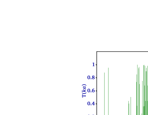
Figure 4: (Color online) Transmission characteristics for a $3$rd generation Vicsek waveguide network. The length of each monomode segment $a$ is chosen as unity.

In Fig. 4, we have shown the two-terminal transmission characteristics for a 3rd generation waveguide network system. The transmission spectrum is, as expected, full of gaps, with resonant transmission exhibited at certain $k$-values. With increasing generation, the resonances become rarer and the spectrum become much more fragmented.

IV Concluding remarks

In conclusion, we have examined the distribution of intensity of light (or any electromagnetic wave) on a Vicsek geometry consisting of diamond shaped single channel waveguides. The major result is that we have been able to identify a countable infinity of localized eigenmodes displaying a multitude of localization lengths. A prescription is given for an exact determination of the wave vectors corresponding to all such modes, a problem that is far from trivial in the case of a deterministically disordered system. The localized wave functions span the fractal space in clusters of increasing sizes, the size being precisely controlled by the length scale at which the wave vector ($k$) is evaluated. The onset of localization can be exactly predicted from the stage of RSRG and can be delayed (staggered) in space. The study provides a unique opportunity to experimentally observe the localization of light triggered by the lattice topology without bothering about the high dielectric constant materials. It may also be useful in developing novel photonic band gap structures, where the wavelengths to be screened or allowed to go through can be controlled over arbitrarily small domains exploiting the fractal character of the network.

- (1) P. W. Anderson, Phys. Rev. 109, 1492 (1958).
- (2) E. Abrahams, P. W. Anderson, D. C. Licciardello, and T. V. Ramakrishnan, Phys. Rev. Lett. 42, 673 (1979).
- (3) A. MacKinnon and B. Kramer, Phys. Rev. Lett. 49, 695 (1982).
- (4) D. J. Thouless, Phys. Rev. Lett. 61, 2141 (1988).
- (5) V. Uski, B. Mehlig, and M. Schreiber, Phys. Rev. B 66, 233104 (2002).
- (6) A. Rodriguez, L. J. Vasquez, K. Slevin, and R. A. Römer, Phys. Rev. Lett. 105, 046403 (2010).
- (7) A. Rodriguez, L. J. Vasquez, K. Slevin, and R. A. Römer, Phys. Rev. B 84, 134209 (2011).
- (8) M. Zilly, O. Ujsághy, M. Woelki, and D. E. Wolf, Phys. Rev. B. 85, 075110 (2012).
- (9) C. Echeverria-Arrondo and E. Ya. Sherman, Phys. Rev. B 85, 085430 (2012).
- (10) T. A. Sedrakyan, J. P. Kestner, and S. Das Sarma, Phys. Rev. A 84, 053621 (2011).
- (11) E. E. Edwards, M. Beeler, T. Hong, and S. L. Rolston, Phys. Rev. Lett. 101, 260402 (2008).
- (12) G. Roati, C. D’Errico, L. Fallani, M. Fattori, C. Fort, M. Zaccanti, G. Modugno, M. Modugno, and M. Inguscio, Nature (London), 453, 895 (2008).
- (13) U. Gavish and Y. Castin, Phys. Rev. Lett. 95, 020401 (2005).
- (14) J. E. Lye, L. Fallani, M. Modugno, D. S. Wiersma, C. Fort, and M. Inguscio, Phys. Rev. Lett. 95, 070401 (2005).
- (15) J. Billy, V. Josse, Z. Zuo, A. Bernard, B. Hambrecht, P. Lugan, D. Clément, L. Sanchez-Palencia, P. Bouyer, and A. Aspect, Nature (London) 453, 891 (2008).
- (16) S. John, Phys. Rev. Lett. 53, 2169 (1984).
- (17) P. W. Anderson, Phil. Mag. B 52, 505 (1985).
- (18) D. M. Jović, M. R. Belić, and C. Denz, Phys. Rev. A 85, 031801(R) (2012).
- (19) K. Y. Bliokh, S. A. Gredeskul, P. Rajan, I. V. Shadrivov, and Y. S. Kivshar, Phys. Rev. B 85, 014205 (2012).
- (20) D. M. Jović, Y. S. Kivshar, C. Denz, and M. R. Belić, Phys. Rev. A 83, 033813 (2011).
- (21) W. Gellermann, M. Kohmoto, B. Sutherland, and P. C. Taylor, Phys. Rev. Lett. 72, 633 (1994).
- (22) A. A. Asatryan, L. C. Botten, M. A. Byrne, V. D. Freilikher, S. A. Gredeskul, I. V. Shadrivov, R. C. McPhedran, and Y. V. Kivshar, Phys. Rev. B 85, 045122 (2012).
- (23) C. H. Hodges and J. Woodhouse, J. Acoust. Soc. Am. 74, 894 (1983).
- (24) S. He and J. D. Maynard, Phys. Rev. Lett. 57, 3171 (1986).
- (25) E. Yablonovitch and T. J. Gmitter, Phys. Rev. Lett. 63, 1950 (1989).
- (26) Z. Shi and A. Z. Genack, Phys. Rev. Lett. 108, 043901 (2012).
- (27) see, Photonic Band Gap Materials, edited by C. M. Soukoulis (Kluwer, Dordrecht, 1995).
- (28) S. John, Phys. Rev. Lett. 58, 2486 (1987).
- (29) E. Yablonovitch, Phys. Rev. Lett. 58, 2059 (1987).
- (30) Z. Q. Zhang, C. C. Wong, K. K. Fung, Y. L. Ho, W. L. Chan, S. C. Kan, T. L. Chan, and N. Cheung, Phys. Rev. Lett. 81, 5540 (1998).
- (31) L. Dobrzynski, A. Akjouj, B. Djafari-Rouhani, J. O. Vasseur, and J. Zemmouri Phys. Rev. B 57, R9388 (1998).
- (32) J. O. Vasseur, B. Djafari-Rouhani, L. Dobrzynski, A. Akjouj, and J. Zemmouri, Phys. Rev. B 59, 13446 (1999).
- (33) R. D. Pradhan and G. H. Watson, Phys. Rev. B 60, 2410 (1999).
- (34) M. Li, Y. Liu, and Z.-Q. Zhang, Phys. Rev. B 61, 16193 (2000).
- (35) S. Sengupta and A. Chakrabarti, Phys. Lett. A 341, 221 (2005).
- (36) S. Sengupta and A. Chakrabarti, Physica E 28, 28 (2005).
- (37) J. Lu, X. Yang, G. Zhang, and L. Cai, Phys. Lett. A 375, 3904 (2011).
- (38) J. Lu, X. Yang, and L. Cai, Optics Comm. 285, 459 (2012).
- (39) E. Domany, S. Alexander, D. Bensimon, and L. P. Kadanoff, Phys. Rev. B 28, 3110 (1983).
- (40) R. Rammal, J. Phys. (Paris) 45, 191 (1984).
- (41) P. Kappertz, R. F. S. Andrade, and H. J. Schellnhuber, Phys. Rev. B 49, 14711 (1994).
- (42) W. A. Schwalm, M. K. Schwalm, Phys. Rev. B 47, 7847 (1993).
- (43) A. Chakrabarti and B. Bhattacharyya, Phys. Rev. B 54, R12625 (1996).
- (44) A. Chakraborti, B. Bhattacharyya, and A. Chakrabarti, Phys. Rev. B 61, 7395 (2000).
- (45) X. R. Wang, Phys. Rev. B 51, 9310 (1995).
- (46) A. Chakrabarti, J. Phys.: Condens. Matt. 8, 10951 (1996).
- (47) E. Maciá, Phys. Rev. B 57, 7661 (1998).
- (48) W. A. Schwalm and B. J. Moritz, Phys. Rev. B 71, 134207 (2005).
- (49) A. Chakrabarti, Phys. Rev. B 72, 134207 (2005).
- (50) B. Pal and A. Chakrabarti, Phys. Rev. B 85, 214203 (2012).
- (51) T. Vicsek, Fractal Growth Phenomena (2nd Ed.), World Scientific, Singapore (1992).
- (52) B. W. Southern, A. A. Kumar, J. A. Ashraff, Phys. Rev. B 28, 1785 (1983).
- (53) S. Alexander, Phys. Rev. B 27, 1541 (1983).
- (54) Z.-Q. Zhang and P. Sheng, Phys. Rev. B 49, 83 (1994).
- (55) A. D. Stone, J. D. Joannopoulos, D. J. Chadi, Phys. Rev. B 24, 5583 (1981)