Measurement of anisotropic radial flow in relativistic heavy ion collisions

Abstract

We suggest the azimuthal distribution of mean transverse (radial) rapidity of the final state particles as a more direct measure of the transverse motion of the source than the standard azimuthal multiplicity distribution. Using a sample generated by the AMPT model with string melting, we demonstrate that the azimuthal amplitude of the suggested distribution characterizes the anisotropic radial flow, and coincides with the parameter of anisotropic radial rapidity extracted from a generalized blast-wave parametrization.

I Introduction

Relativistic heavy ion collisions provide a way to study the properties of strongly interacting matter. The observation of large elliptic flow at RHIC is considered one of the most important signatures for the formation of the strongly interacting Quark Gluon Plasma (sQGP) qgp ; gulassys . The flow harmonics are Fourier coefficients of the azimuthal multiplicity distribution of final state hadrons v2 . They are considered sensitive probes of the evolution of the system formed in relativistic heavy ion collisions Arthur .

One common feature of flow harmonics is their mass ordering in the low transverse momentum region Arthur . This phenomena can be well understood by hydrodynamics with a set of kinetic freeze-out constraints, i.e., the temperature, the radial flow, and the source deformation Heinz-PLB . The radial flow is usually described by 2 parameters. The first is the isotropic radial velocity (or rapidity, $v_{\rm T}=\tanh y_{\rm T}$). It presents the surface profile of isotropic transverse expansion of the source at kinetic freeze-out.

The other parameter is the anisotropic radial velocity (i.e., the azimuthal dependent radial velocity). It measures the difference of the radial flow strength in and out of the reaction plane. It is introduced to account for the anisotropic radial flow field which arises in non-central collisions. The observed elliptic flow can be generated by anisotropic radial flow Heinz-PLB ; Lisa . Moreover, the shear tension of viscous in hydrodynamics is supposed to be proportional to the gradient of radial velocity along the azimuthal direction Landao , which is directly related to anisotropic radial velocity. The proportionality constant is the shear viscosity.

In hydrodynamic model Kolb ; Huovinen ; Huichao Song , these parameters are not independent. They are related by the initial conditions and the equation of state and their determination is crucial for theoretical calculations.

The azimuthal distribution of the mean transverse rapidity of final state hadrons ($\langle y_{\rm T}(\phi)\rangle$) directly measures the transverse motion of the source at kinetic freeze-out lilin-cpc . It should be helpful in determining the parameters of the anisotropic radial rapidity. In contrast to the azimuthal multiplicity distribution, where only the number of particles is concerned, here the average is over all particles in a given azimuthal direction. The influence of the number of particles is excluded.

As we know, $\langle y_{\rm T}(\phi)\rangle$ should contain three parts: average isotropic radial rapidity, average anisotropic radial rapidity, and average thermal motion rapidity Arthur . Since both thermal and radial motions contribute to the isotropic rapidity of the distribution, the isotropic radial rapidity itself can not be directly obtained from the distribution. So conventionally, the radial flow parameters are extracted from the $p_{\rm T}$ spectra of the hadrons Schnedermann ; Broniowski , or dileptons Jajati ; Mohanty , by generalized blast-wave parametrizationHeinz-PLB ; Lisa .

Fortunately, the thermal motion is isotropic. As such, it does not contribute to the anisotropic radial flow. The azimuthal amplitude of the mean transverse rapidity distribution should correspond directly to the anisotropic radial rapidity. It is interesting to see the features of the azimuthal distribution of mean transverse rapidity, and how its azimuthal amplitude relates to the parameters of anisotropic radial rapidity extracted by a generalized blast-wave parametrization.

In the paper, we define the $\langle y_{\rm T}(\phi)\rangle$ in section II. Using a sample generated by the AMPT model with string melting  ampt1 ; ampt2 , the suggested distribution and its particle mass and centrality dependence are presented. These show that the isotropic and anisotropic parts of the suggested distribution behave as the expected radial flow (with a random thermal component), and anisotropic radial flow, respectively. In section III, the $p_{\rm T}$ spectra of 6 particle species and their corresponding elliptic flows, $v_{2}(p_{\rm T})$, are presented. Fitting these spectra and elliptic flows by a generalized blast-wave parametrization, the temperature, and the radial flow parameters are obtained. It is found that the parameter of anisotropic radial rapidity is well described by the azimuthal amplitude of the suggested distribution. Finally, the summary and conclusions are given in section IV.

II Azimuthal distribution of mean transverse rapidity

Usually, the transverse rapidity of a final state hadron is considered a good approximation of its transverse rapidity at kinetic freeze-out nature . It is defined as,

$$y_{\rm T}=\ln(\frac{m_{\rm T}+p_{\rm T}}{m_{0}})$$ (1)

where $m_{0}$ is the particle mass in the rest frame, $p_{\rm T}$ is transverse momentum, and $m_{\rm T}=\sqrt{m_{0}^{2}+p_{\rm T}^{2}}$ is the transverse mass. The mean transverse rapidity in a given azimuthal angle bin is defined as the summation of all particles’ rapidities divided by the total number of particles, i.e.,

$$\langle y_{\rm T}(\phi-\psi_{r})\rangle=\frac{1}{N_{\mathrm{event}}}\sum_{e=1}^{N_{\mathrm{event}}}\frac{1}{N^{e}_{m}}\sum_{i=1}^{N^{e}_{m}}y_{{\rm T},i}^{e}(\phi_{m}-\psi_{r}),$$ (2)

where $y_{T,i}^{e}$ is the transverse rapidity of the $i$th particle and $N_{m}^{e}$ is the total number of particles in $m$th azimuthal angle bin in $e$th event. The direction of reaction plane is given by $\psi_{r}$, which is zero in model calculation, and can be determined in experiment by 3 similar ways as that for the azimuthal multiplicity distribution arthur. By definition, the influence from the number of particles is therefore removed. Eq. (2) measures the mean transverse motion in azimuthal direction lilin-cpc .

In order to see the generic features of the defined distribution, we present the distribution from a sample of Au + Au collisions at 200 GeV generated by the AMPT model with string melting ampt2 in Fig. 1(a). For the following comparison, we use a longitudinal rapidity window of $|y_{\rm L}|<0.1$, the same as published spectra data from the STAR experiment STAR-v2 ; Abelev .

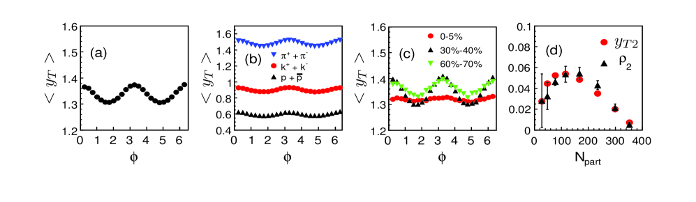
Figure 1: (Color online) (a) $\langle y_{\rm T}(\phi)\rangle$ of minimum bias sample, (b)$\langle y_{\rm T}(\phi)\rangle$ for 3 different mass particles, (c) $\langle y_{\rm T}(\phi)\rangle$ at three different centralities, $0-5\%$ (red points), $30\%-40\%$ (black triangles), and $60\%-70\%$ (green down triangles), (d) The centrality dependence of $y_{T2}$ (red points), and $\rho_{2}$ (black triangles).

From the figure, we can see it is a periodic function of azimuthal angle and can be well fitted by,

$$\langle y_{\rm T}(\phi)\rangle=y_{\rm T0}+y_{\rm T2}\cos(2\phi).$$ (3)

Eq. (3) consists of two parts: an isotropic mean rapidity, $y_{\rm T0}=1.3371\pm 0.0001$, and a mean azimuthal dependent rapidity amplitude, $y_{\rm T2}=0.0334\pm 0.0002$. This directly indicates the anisotropic distribution of transverse motion, in addition to the known anisotropy distribution of particle number. Further, the anisotropic amplitude, $y_{\rm T2}$, should correspond to the parameter of anisotropic radial rapidity.

The isotropic part is a combination of radial rapidity and thermal motion rapidity. As we know, the thermal motion is mainly determined by the temperature and particle mass. For a system at fixed temperature, the lighter particles should have larger thermal velocity. To see this feature in isotropic rapidity we plot the distributions of three different particle species, $\pi$, $k$, and $p$ in Fig. 1(b). It shows that the lightest particles (pions) have the largest isotropic rapidities, while the heaviest particles (protons) have the smallest isotropic rapidities, and intermediate mass particles (kaons) have rapidities between them. These indicate that their isotropic rapidities are ordered as expected from random thermal motion.

To see the influence of centrality on the anisotropic part, the azimuthal distributions of mean transverse rapidity at three typical centralities, $0-5\%$, $30\%-40\%$, and $60\%-70\%$, are presented in Fig 1(c). From the figure, we can see that the distributions are azimuthal angle dependent in non-central collisions, i.e., the mid-central and peripheral collisions with centralities of $30\%-40\%$ and $60\%-70\%$. It becomes almost flat and azimuthal angle independent in central collisions ($0-5\%$). So the azimuthal dependent part of the distribution appears only in non-central collisions.

This is consistent with the fact that only two parameters, the temperature and radial rapidity, are required to describe the observed $p_{\rm T}$ spectra in central collisions, as done in early blast-wave parametrization Lisa . However, the parameter of anisotropic radial flow is necessary for non-central collisions Heinz-PLB ; Lisa .

The centrality dependence of the azimuthal amplitude, $y_{\rm T2}$, is shown in Fig. 1(d) by red solid circles. It has a maximum in mid-central collisions, decreases toward peripheral and central collisions, and is close to zero in central collisions.

The disappearance of $y_{\rm T2}$ in central collisions also indicates that the thermal motion, which exists in central collisions as well, is isotropic and does not contribute to the anisotropic radial rapidity. Therefore, the azimuthal amplitude of the suggested distribution describes the parameter of anisotropic radial rapidity. In order to show this quantitatively, we will compare it with the parameter that is extracted from the same sample by a generalized blast-wave parametrization in the following section.

III The parameters of radial flow

The blast-wave model is currently the only model that simply includes the radial flow parameters. It is motivated from hydrodynamics with the kinetic freeze-out parameters Lisa ; Schnedermann ; Siemens ; STAR-v2 ; Adams2 ; blast-v2 . It is assumed that the longitudinal expansion is boost invariant Bjorken . The single-particle spectrum is given by the Cooper-Frye formalism (as in hydrodynamics) Cooper ,

$$E\frac{d^{3}N}{d^{3}p}\propto\frac{1}{(2\pi)^{3}}\int_{\Sigma_{f}}{p^{\mu}d\sigma_{\mu}(x)f(x,p)},$$ (4)

where $f(x,p)$ is the momentum distribution at space-time point $x$. Eq. (4) is an integral over a freeze-out hyper-surface, and sums over the contributions from all space-time points.

Originally, local thermal equilibrium is assumed to be reached at kinetic freeze-out and a Boltzman distribution of the momentum is applied Schnedermann . It has been shown recently that a Tsallis distribution provides an even better description for all $p_{\rm T}$ spectra from elementary to nuclear collisions Tsallis ; Shao . So, we use the Tsallis distribution for $f(x,p)$, i.e.,

$$f(x,p)=\Biggl{[}1+\frac{q-1}{T(x)}\biggl{(}p\cdot\hfill\break u(x)-\mu(x)\biggr{)}\Biggr{]}^{-\frac{1}{q-1}},$$ (5)

where $q$ is the parameter characterizing the degree of non-equilibrium, and $T$ is the kinetic freeze-out temperature. Thus the transverse momentum spectrum can be given by Tang ,

$$\frac{dN}{p_{\rm T}dp_{\rm T}d\phi} \propto \int_{0}^{2\pi}d\phi_{s}\int_{-y_{b}}^{y_{b}}dye^{\sqrt{y_{b}^{2}-y^{2}}}\cosh y\int_{0}^{R}m_{\rm T}rdr$$ (6)

$$\ \ \Biggl{[}1+\frac{q-1}{T}\biggl{(}m_{\rm T}\cosh y\cosh\rho$$

$$\qquad-p_{\rm T}\sinh\rho\cos(\phi_{b}-\phi)\biggr{)}\Biggr{]}^{-\frac{1}{q-1}}$$

where $m_{\rm T}$ and $p_{\rm T}$ are transverse mass and transverse momentum of the particle, respectively, and $y_{b}=\ln(\sqrt{s_{NN}}/m_{N})$ is the beam rapidity Wong .

According to the generalized blast-wave parametrization, the radial flow rapidity which controls the magnitude of the transverse expansion velocity is Lisa ; Poskanzer ; STAR-v2 ; Yongseok ,

$$\rho=\widetilde{r}\bigl{(}\rho_{0}+\rho_{2}\cos(2\phi_{b})\bigr{)}$$ (7)

where $\widetilde{r}=\sqrt{(r\cos(\phi_{s})/R_{X})^{2}+(r\sin(\phi_{s})/R_{Y})^{2}}$. $\rho_{0}$ is the isotropic radial flow rapidity, and $\rho_{2}$ is the amplitude of the anisotropic radial flow rapidity, respectively. The greater the magnitude of $\rho_{2}$, the larger the momentum-space anisotropy. Here, $\phi_{s}$ is the azimuthal angle in coordinate space and $\phi_{b}$ is the azimuthal angle of the boost source element defined with respect to the reaction plane. They are related by $\tan(\phi_{b})=(R_{X}/R_{Y})^{2}\tan(\phi_{s})$.

There are 5 undetermined parameters: the temperature ($T$), isotropic radial flow rapidity ($\rho_{0}$) and anisotropic radial flow rapidity ($\rho_{2}$), $q$ of the Tsallis distribution, and $R_{X}/R_{Y}$. Since all the particles are assumed to move with a common radial flow velocity, the mean kinetic freeze-out parameters are usually obtained by the simultaneous fitting of spectra from several hadrons  Abelev ; Adams2 and elliptic flow Lisa . Elliptic flow, $v_{2}(p_{\rm T}$), is the second coefficient of the Fourier expansion of azimuthal multiplicity distribution Ollitrault1 ; Voloshin , and defined as,

$$v_{2}(p_{\rm T})=\frac{\int_{-y_{b}}^{y_{b}}dy\int_{0}^{2\pi}d\phi\cos(2\phi)\frac{dN}{p_{\rm T}dp_{\rm T}dyd\phi}}{\int_{-y_{b}}^{y_{b}}dy\int_{0}^{2\pi}d\phi\frac{dN}{p_{\rm T}dp_{\rm T}dyd\phi}}.$$ (8)

In Fig. 2, the $p_{\rm T}$ spectra of six particles, $\pi^{\pm}$, $K^{\pm}$, $\overline{p}$, and $p$, of the same sample, are presented by red solid circles. The differential elliptic flow $v_{2}(p_{\rm T})$ of pions, kaons, and protons are presented in Fig. 3 by black triangles, red solid circles and blue triangles, respectively. The error bars only include statistical errors. They are very small in comparison with the experimental data STAR-v2 . Typically, the systematic errors are considered to be $5\%$ when fitting the simulated data Shan . Due to resonance decays in the low momentum region of pions Abelev , the data points in the low $p_{\rm T}$ regions of the spectra are excluded in this fitting.

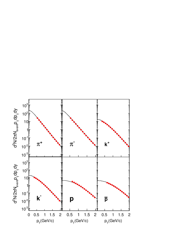
Figure 2: (Color online) The transverse momentum spectra for $\pi^{\pm}$, $K^{\pm}$, $\overline{p}$ and $p$ within $|y_{\rm L}|<0.1$ for the sample of Au+Au collisions at $\sqrt{s_{NN}}=200$ GeV generated by the AMPT model with string melting.

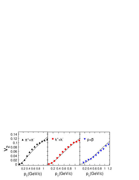
Figure 3: (Color online) The differential elliptic flow $v_{2}(p_{T})$ for different particle species within $|y_{\rm L}|<0.1$ for the sample of Au+Au collisions at $\sqrt{s_{NN}}=200$ GeV generated by the AMPT model with string melting.

Using Eqs. (6), and (8), the fitting curves in each plots of Fig. 2 and 3 are drawn. They describe well the corresponding data points of the $p_{\rm T}$ spectra and elliptic flow. The fitting parameters are $T=96.1\pm 1.0(MeV)$, $\rho_{0}=0.73\pm 0.01$, and $\rho_{2}=0.035\pm 0.003$. This temperature is the same magnitude as that given by hydrodynamics Heinz-PLB ; Huichao Song , and experimental data STAR-v2 . The parameter of anisotropic radial flow rapidity, $\rho_{2}$, is very close to the azimuthal amplitude of the suggested distribution, $y_{\rm T2}=0.0334\pm 0.0002$.

The centrality dependence of $\rho_{2}$ is shown in Fig. 1(d) by black triangles. We can see that at each centrality, $\rho_{2}$ is very close to $y_{\rm T2}$. The azimuthal amplitude of the suggested distribution coincides with the parameter of anisotropic radial flow rapidity extracted from a generalized blast-wave parametrization.

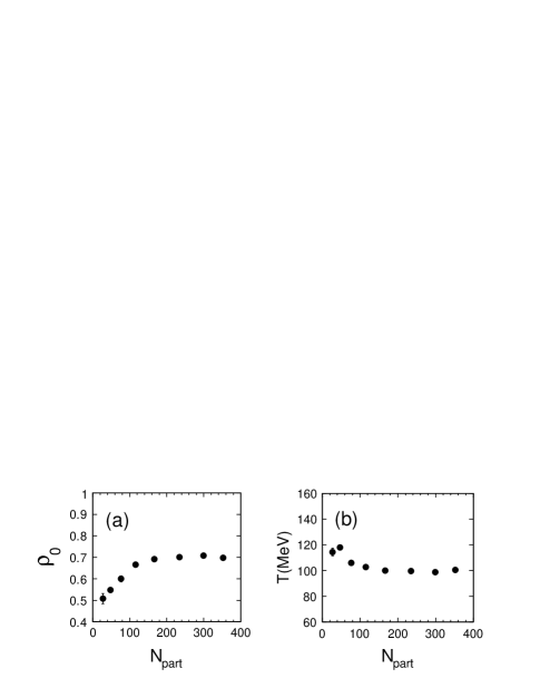
Figure 4: The centrality dependence of (a) the isotropic radial flow rapidity and (b) the temperature obtained by blast-wave parametrization from the sample of Au+Au collisions at 200 GeV generated by the AMPT model with string melting.

To complete the discussion of the fitting, the centrality dependence of $\rho_{0}$ and $T$ are shown in Figs. 4(a) and (b), respectively. We can see that $\rho_{0}$ increases with the increasing of number of participants, and reaches a maximum in central collisions. The temperature changes with centrality in the opposite way as that of radial flow, $\rho_{0}$. The radial flow and the temperature are negatively correlated, as expected Schnedermann ; Bearden . This is because the produced hadrons in central collisions have more time to cool down, rescatter, and form a stronger radial expansion flow. In peripheral collisions, there is not enough time to convert thermal energy to the collective flow motion.

IV Summary and conclusions

In this paper the measurement of the azimuthal distribution of mean transverse rapidity of final state hadrons is proposed as a more direct probe of the transverse motion of the source than the known azimuthal multiplicity distribution.

Using the sample generated by the AMPT model with string melting, we show that the isotropic part of the distribution is a combination of the radial and thermal motions. The azimuthally dependent part measures the anisotropy of transverse motion arising from non-central collisions.

Using a generalized blast-wave parametrization, we further extract the temperature and radial flow parameters from the same sample. It is found that the parameter of anisotropic radial rapidity coincides with the azimuthal amplitude of the suggested distribution.

The $\langle y_{\rm T}(\phi)\rangle$ provides a direct measurement of the anisotropic radial rapidity. This is important for hydrodynamic calculations and for a direct measurement of shear viscosity in relativistic heavy ion collisions Meijuan .

V Acknowledgement

We are grateful for the valuable comments of Dr. Zhangbu Xu, Fuqiang Wang and Terence Tarnowsky. The first author would thank Dr. Zebo Tang for effective helps in using Tsallis distribution. This work is supported in part by the NSFC of China with project No. 10835005 and 11221504, and MOE of China with project No. IRT0624 and No. B08033.

References

- (1) K. Adcox et al.(PHENIX Collaboration), Nucl. Phys. A757, 184-283(2005); John Adams et al.(STAR Collaboration), Nucl.Phys.A757, 102-183(2005); B. B. Back et al.(PHOBOS Collaboration), Nucl. Phys. A757, 28-101(2005); I. Arsene et al.(BRAHMS Collaboration), Nucl. Phys. A757, 1-27(2005).
- (2) Miklos Gyulassy, Larry McLerran, Nucl. Phys. A750 30-63(2005). B. Müller, Annu. Rev. Nucl. and Part. Phys., 1(2006).
- (3) J. Y. Ollitrault, Phys. Rev. D 46, 229 (1992); H. Sorge, Phys. Rev. Lett. 78, 2309 (1997); K.H. Ackermann et al., STAR Collaboration, Phys. Rev. Lett. 86, 402 (2001); Adams et al. (STAR Collaboration), Phys. Rev. Lett. 92, 052302 (2004).
- (4) Sergei A. Voloshin, Arthur M. Poskanzer, and Raimond Snellings, arXiv: 0809.2949.
- (5) P. Huovinen, P.F. Kolb, U. Heinz, P.V. Ruuskanen and S. Voloshin, Phys. Lett. B 503, 58 (2001).
- (6) F. Retiere and M.A. Lisa, Phys. Rev. C 70, 044907 (2004).
- (7) L.D.Landau, E.M. Lifschitz, Fluid Mechanics, Insti- tute of Physical Problems, U.S.S.R. Academy of Sci- ences,Volume 6, Course of Theoretical Physics.
- (8) P.F. Kolb, J. Sollfrank, U. Heinz, Phys. Lett. B 459, 667 (1999).
- (9) P. Huovinen and P. V. Ruuskanen, Ann. Rev. Nucl. Part. Sci. 56, 163 (2006). D. A. Teaney, arXiv: 0905.2433.
- (10) Huichao Song, arXiv:0908.3656.
- (11) Li Lin, Li Na and Wu Yuanfang, Chinese Physics C 36, 423 (2012).
- (12) E. Schnedermann, J. Sollfrank, and U. W. Heinz, Phys. Rev. C 48, 2462 (1993).
- (13) W.Broniowski and W.Florkowski. Phys. Rev. Lett. 87, 272302 (2001).
- (14) Jajati K. Nayak and Jan-e Alam, Phys. Rev. C 80, 064906 (2009).
- (15) Payal Mohanty, Jajati K Nayak, Jan-e Alam and Santosh K Das, arXiv: 0910:4856.
- (16) B. Zhang, C.M. Ko, B.A. Li and Z.W. Lin, Phys. Rev. C 61, 067901 (2000).
- (17) Zi-Wei Lin, Che Ming Ko, Bao-An Li, Bin Zhang and Subrata Pal, Phys. Rev. C 72, 064901 (2005).
- (18) P. Braun-Munzinger, J. Stachel, Nature 448 Issue 7151, 302-309 (2007).
- (19) J. Adams et al.(STAR Collaboration),Phys.Rev.C 72, 014904 (2005).
- (20) B.I.Abelev et al (STAR Collaboration) Phys. Rev. C 79, 034909 (2009).
- (21) J. Adams et al., Phys. Rev. Lett. 92, 112301 (2004).
- (22) W. Broniowski, A. Baran, W. Florkowski, AIP Conf. Proc. 660, 185 C195 (2003), nucl-th/0212053.
- (23) P. Siemens and J.O. Rasmussen, Phys. Rev. Lett. 42, 880 (1979).
- (24) J. D. Bjorken, Phys. Rev. D 27, 140 (1983).
- (25) F. Cooper and G. Frye, Phys. Rev. D 10, 186 (1974).
- (26) C. Tsallis, J. Stat. Phys. 52, 479 (1988).
- (27) Ming Shao, Li Yi, Zebo Tang, Hongfang Chen et al., J.Phys.G 37, 085104 (2010).
- (28) Zebo Tang et al.,arXiv: 1101.1912.
- (29) C.-Y. Wong, Phys. Rev. C 78, 054902 (2008).
- (30) Arthur M. Poskanzer, J.Phys. G 30, S1225-S1228 (2004).
- (31) Yongseok Oh, Zi-Wei Lin, Che Ming Ko, Phys. Rev. C 80, 064902 (2009).
- (32) J.-Y. Ollitrault, Phys. Rev. D 46, 229 (1992).
- (33) S. Voloshin, Y. Zhang, Z. Phys. C 70, 665 (1996).
- (34) Shan Lianqiang. J.Phys.G:Nucl.Part.Phys. 36, 055003 (2009).
- (35) Bearden I G et al (NA44 Collaboration) Phys. Rev. Lett. C 78, 2080 (1997).
- (36) Wang Meijuan, Li Lin, Liu Lianshou and Wu Yuanfang, J. Phys. G: Nucl. Part. Phys. 36, 064070(2009).