Effects of Asymmetric Flows in Solar Convection on Oscillation Modes

Abstract

Many helioseismic measurements suffer from substantial systematic errors. A particularly frustrating one is that time-distance measurements suffer from a large center to limb effect which looks very similar to the finite light travel time, except that the magnitude depends on the observable used and can have the opposite sign (Zhao et al., 2012). This has frustrated attempts to determine the deep meridional flow in the solar convection zone, with Zhao et al. (2012) applying an ad hoc correction with little physical basis to correct the data. In this letter we propose that part of this effect can be explained by the highly asymmetrical nature of the solar granulation which results in what appears to the oscillation modes as a net radial flow, thereby imparting a phase shift on the modes as a function of observing height and thus heliocentric angle.

1. Introduction

The meridional flow in the solar convection zone plays a key role in many solar dynamo models and an accurate measurement of the flow with depth and latitude would thus be invaluable for constraining solar dynamo models. There have been numerous attempts to obtain estimates using a variety of techniques, including time-distance (Giles, 2000; Zhao et al., 2012, in the following Z12), ring diagrams (Schou & Bogart, 1998; Haber et al., 2002), normal modes (Woodard et al., 2012, in the following W12), and supergranulation studies (Hathaway, 2011). While these studies have given reasonable numbers near the surface, they have suffered from large and unexplained systematic errors, preventing us from obtaining reliable numbers throughout the convection zone.

A meridional counter-cell at high latitude was first found by Haber et al. (2002); subsequent work (González Hernández et al., 2006; Zaatri et al., 2006) found this to be a periodic phenomena tightly correlated with the solar inclination angle ($B_{0}$). Zaatri et al. (2006), concluding that the counter-cells were likely spurious, applied a correction to remove them. Braun & Birch (2008) found that North–South travel times differed depending on the heliocentric longitude at which the measurement was performed. Most recently, Z12 used data from the Helioseismic and Magnetic Imager (HMI) to measure East–West travel time shifts along the equator and North–South travel time shifts along the central meridian in four different observables: continuum intensity, line core intensity, line depth (continuum minus line core), and Doppler velocity. They found large E–W travel time shifts along the equator, and found that they were quite different in different observables.

Although Z12 did not provide an explanation for the source of the error, they treated it as a heliocentric angle dependent phase or time shift. Using this assumption, they used the E–W travel time anomalies to correct the N–S travel time shifts — this brought the four different observables into good agreement, which was encouraging. Similarly, it was noted by W12 that a radially varying phase of the eigenfunctions coupled with the variation in the height of formation with changing heliocentric angle might be an explanation, but again no source of such a phase variation was identified.

It is evident that helioseismic observations should suffer from a phase error as a function of heliocentric angle — as Duvall & Hanasoge (2009) pointed out, the light travel time for an observation at disk center is different than for an observation near the limb by roughly 2s. When analyzing travel time residuals, however, they found the correct magnitude but opposite sign. They conlcuded that the measured travel times suffer from a systematic effect with twice the magnitude and opposite sign as the expected light travel time effect. Similar numbers were found by Schou et al. (2012), who found that a travel time error of 2–3s at a heliocentric angle of 60^∘ could explain their results.

In general, standing acoustic waves should have a constant phase with height. Many effects that are known to be poorly modeled or neglected entirely do not change this. What is required to add a phase shift with height is an asymmetric effect, e.g. an effect which knows whether a wave is traveling upwards or downwards. In the Sun, of course, the modes we observe are not purely standing, and mode damping due to, for example, non-adiabatic effects will have an effect. In this work we are considering low frequencies, however, so we neglect this.

Here we suggest that a phase variation arises from the large asymmetry between the upflows and downflows in the convection near the solar surface. In particular, the broad upflows and narrow downflows give rise to net vertical flows when horizontally averaged over length scales much smaller than the acoustic modes. As was shown by Gough & Hindman (2010) in the context of meridional flows, a flow introduces a phase shift in acoustic modes — one would expect the vertical convective flows in the Sun to introduce a phase shift with height in the solar atmosphere.

In the following discussion, we extract complex eigenfunctions from a detailed numerical simulation of convection to compute the phase delay as a function of height. We attempt to explain this phase shift as being due to the spatially averaged vertical flows by computing phases shifts to theoretical eigenfunctions with an imposed vertical flow and comparing these to the numerical eigenfunctions from the simulation. We use the phase shifts from the simulation data to predict systematic effects in travel-time measurements as a function of distance from disk center, and compare these effects to the observed discrepancies in solar data. Finally, we discuss some of the shortcomings of our models, how they might be improved, and discuss other observable consequences.

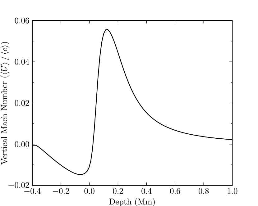
Figure 1.— Mach number as a function of depth from a model by Stein et al. (2009). The area average of the flow divided by the area average of the sound speed is used. To exclude the buffer zone used in the model the outer 5 grid points were excluded. The Mach number below 1Mm is negligible.

2. Models

We use a non-magnetic simulation of solar convection (Stein et al., 2009). Convection in the outer layers of the solar envelope and atmosphere are simulated in a small Cartesian box. We show the horizontally averaged vertical Mach number in Figure 1. In this work we assume that the modes ‘see’ only this horizontal average. For low degree modes, this is likely to be an adequate approximation for our purposes.

2.1. Simulation Results

The phase shifts of the eigenfunctions can be estimated by extracting them from a convection simulation, as previously done (Stein & Nordlund, 2001), but this time including the imaginary component. This is easily done by horizontally averaging the vertical velocity (to isolate radial modes) from such a simulation and taking a temporal Fourier transform at each depth. The phase shifts can be converted to time delays by dividing by the angular frequency $\omega$. Results of such an analysis are shown in Figure 2 for the two lowest frequency modes (those at higher $n$ are less well defined).

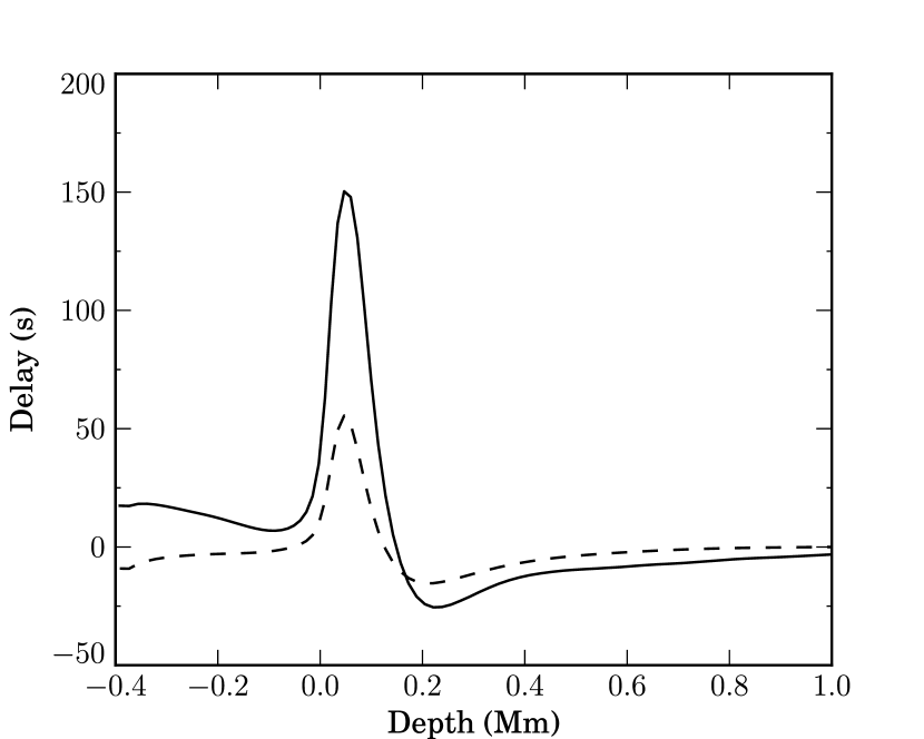
Figure 2.— Time delay as a function of depth from the simulation. Solid line is for lowest $n$ at 1142$\mu$Hz, dashed for the second lowest $n$ at 1761$\mu$Hz.

2.2. Explaining the Simulation Results: Theoretical Eigenfunctions

What is the cause of the phase shift we see in the standing waves in the simulation box? To get a crude estimate of the effect of the vertical flows, we start by considering the wind-in-a-pipe model of Gough & Hindman (2010), Section 3. Manipulating their equations and extending their Equation (9) to allow all variables to depend on position shows that the time shift introduced by a flow is given by

$$\Delta\tau(x)=\int_{x1}^{x2}\frac{U(x)}{c(x)^{2}}dx=\int_{x1}^{x2}\frac{M(x)}{c(x)}dx,$$ (1)

where $x$ is the distance from the end of the pipe. The results of this calculation are shown in Figure 3. It will be noted that, while some features of the numerical eigenfunctions are qualitatively reproduced (i.e. a negative slope in the atmosphere and a steeper positive slope just below the photosphere), there is a quantitative disagreement of more than an order of magnitude. This is not surprising, however, as this toy model assumes that the background model varies slowly compared to the wavelength, and that is manifestly not the case here.

A somewhat more sophisticated approach is to compute the oscillation eigenfunctions for a stellar envelope with a specified vertical flow $U(r)$. To do this, we perturb the equations of continuity, motion, and energy in the usual way (following, e.g., Unno et al., 1989), but with the added velocity term in the base equations. For simplicity, we consider only radial modes in this work, but the generalization to non-radial modes is straightforward. When a vertical flow is present, the solutions become complex, and we can compute a phase delay as a function of height.

By including only a horizontally averaged vertical flow, we are of course involving a certain physical inconsistency — that is, a horizontally invariant vertical flow is not consistent with a one dimensional background model, which requires a zero net mass flux. Because we are computing eigenfunctions in the linear perturbative regime, this is not necessarily an unreasonable inconsistency to accept, but it does require that we employ certain assumptions. As noted above, we assume here that the modes ‘see’ the horizontal spatial average of the convective flows. One consequence of this assumption is that we assume that variations on convective length scales (horizontally) do not affect the acoustic modes. For radial modes this is reasonable. It also also assumes that the correlations between flows and thermodynamic quantities — say, density — do not have an effect on the phases of these modes.

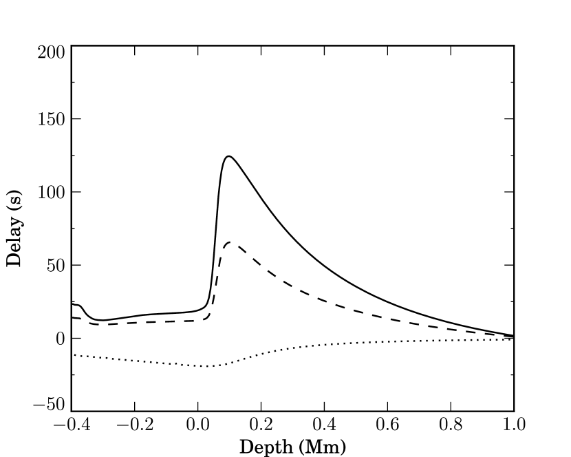
Figure 3.— Predicted effect of vertical velocity on mode eigenfunctions. The dotted line shows the result of integrating Equation 1, multiplied by a factor of 10 to that it can be seen on this scale. The solid and dashed lines show the predictions from a more detailed calculation, at 1142 $\mu$Hz and 1761 $\mu$Hz, respectively.

Using the horizontally averaged thermodynamic quantities and vertical flow from the simulation box, we integrate the oscillation equations for radial modes with frequencies of 1142$\mu$Hz, and 1761$\mu$Hz, which may be directly compared with the eigenfunction phases shifts shown in Figure 2. The calculated eigenfunction phase shifts are shown in Figure 3. As can be seen, there is a general qualitative agreement between the two sets of phase delays. Most prominently, we see a strong positive phase shift just below the photosphere, though we calculate a somewhat smaller shift, and also find the peak to be much broader below the surface. In the atmosphere itself we find a fairly constant phase, or a slight phase lag with height. This is not entirely in agreement with the numerical eigenfunctions, but there is some uncertainty in the numerical eigenfunctions due to noise. We consider the agreement to be sufficiently good to conclude that the phase shifts we observe in the convection simulations are due to the vertical convective flows.

2.3. Effects on observations

The HMI instrument measures, among other things, continuum intensity, line core intensity, and line-of-sight velocity. These observables are produced at a range of heights in the solar atmosphere (Fleck et al., 2011), and can be represented as the convolution of some contribution function of height and the actual variation of the quantity in the solar atmosphere. A contribution function for the HMI line core intensity measurements can be found in Fleck et al. (2011, Figure 2); the other observables have contribution functions that peak at different heights. The contribution function can be approximated by a Gaussian with a width of 250km. We will use this in the work that follows. A detailed study of the contribution function of the various HMI observables as a function of viewing angle is far beyond the scope of this letter.

To relate the change with height to the change with viewing angle we need to determine the relationship between these two quantities. Assuming that the atmosphere is isothermal and that the height of formation corresponds to the place where a certain column density of matter has been traversed from infinity, it can easily be shown that the change in height with angle is given by $\Delta h=-H\log(\cos(\theta))$, where $H\approx$120 km is the density scale height and $\theta$ is the angle between vertical and the line of sight. At $\theta=60^{\circ}$ this corresponds to about 80km.

In Figure 4 we show the time delays integrated over a Gaussian contribution function as a function of viewing angle for various disk-center formation heights. We also show the derivatives with respect to angular distance from disk center of the time delays. These derivatives give the travel time differences one would measure in the limit of infinitely small apperture size, and can provide a good approximation for the apperture sizes used in Z12. For direct comparison with Z12, the values of our derivatives must be multiplied by the apperture size used in the measurement.

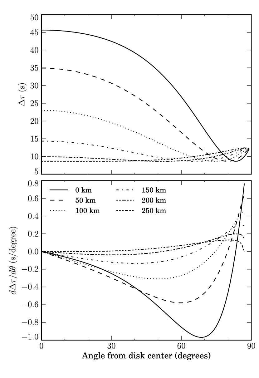
Figure 4.— Phase shifts as a function of viewing angle for different disk center formation heights, integrated over a Gaussian contribution function. The width of the Gaussian is 250km, chosen to match the contribution function from Fleck et al. (2011). The top panel shows the phases at different viewing angles; the bottom panel shows the derivative of the phases with viewing angle.

3. Discussion

We have explored the effects of vertical convective flows on solar acoustic modes. Can they explain the systematics that have been observed in solar data, for example the effect found in Z12? In that work, the authors showed East-West travel time differences across the the solar equator for different HMI observables (line-of-sight velocity, continuum intensity, line core intensity, and line depth). They found that all observables exhibited systematic effects along the equator that they believed to be spurious, but that each different observables had different signatures. Comparing their Figure 2 with the bottom panel of our Figure 4, we note some striking similarities. First, the continuum shows the largest anomaly — as does the 0km height measurement we predict, and with the same sign (negative). The Doppler signal, with a peak in the contribution function at approximately 150km, shows a much smaller anomaly but still the same sign. We predict the same thing (note that our 150km signal changes sign, but only above 60^∘ from disk center, which is further than the Z12 results go. Finally the line core intensity, with the highest formation height (250km), shows an anomaly with the opposite sign, and this is matched by our results. Furthermore, the Z12 anomalies show turnovers as the distance from disk center gets large, and we show the same.

The quantitative agreement is not as promising, however. In particular, the magnitude of the effect we predict, by multiplying the derivative of the phase shifts by the aperture size used in the measurements, is too small — at most a few seconds, as opposed to the more than 10 seconds Z12 find in continuum intensity. Furthermore, while we do predict the turnover observed, we do not accurately predict where this should happen.

Several approximations may be identified, some of which are easily amenable to improvement and others not. First of all the use of the area weighted vertical velocity is unlikely to be correct. In reality the propagation of waves in a medium with small scale ($\ll$ wavelength) variations is a complicated issue and the velocities would likely have to be weighted in some other way. In particular, variations in different quantities (significantly density and velocity) are correlated, which will need to be taken into account.

Another problem is that the granulation is not static on the timescale of the oscillations and that there are likely to be interactions between the two. This should be well captured by the simulations, but is probably difficult to model accurately — at least for the present authors.

Finally we have ignored complex issues of radiative transfer. In approximating the contribution function as a Gaussian, we have simplified the problem but done violence to the actual physics. For the present purposes we consider it sufficient, but the exact shape of the actual contribution functions (which are different both for different observables and for the same observable at different viewing angles) will have significant quantitative effects. It is not likely, however, that the qualitative results would be affected. At least this problem is well understood and has been addressed in detail for other purposes.

In addition to the phase shift with observing angle, there are other possible observational consequences. Perhaps most obviously there will be a phase shift between different observables, such as continuum intensity and Doppler shift, which might be misinterpreted as a propagation or non-adiabaticity effect.

Another effect is that even for the same observable there should be a phase difference between observation heights. This includes, e.g., Doppler shifts derived from different parts of the spectral line and even observations in the middle of granulation versus intergranular lanes.

In addition to the observational effects, the fact that eigenfunctions can be determined with significant accuracy from numerical simulations presents many opportunities, in particular ones involving the ability to determine if the depth variation of both the real and imaginary parts match models. Potentially this could be used to test models of the interaction of waves with granulation and non-adiabatic effects, hopefully leading to a better understanding of the physics behind such things as the surface terms currently being applied in an ad hoc way in structure inversions.

4. Conclusion

We have shown that the effect of the vertical flows from convection in the outer solar convection zone and atmosphere do affect the quantities we observe in helioseismology. We have further shown that the systematic errors that have been observed can be qualitatively explained by this effect. We conclude that the ad hoc correction applied by Z12 is likely justified.

A full quantitative prediction of the effects of the vertical flows requires a more sophisticated effort than that employed in this work. In particular, the modeling of the structure of the atmosphere must be very accurate and a proper treatment of the actual measurements we take must be done. This work, while non-trivial, is certainly feasible, and would be useful in addressing a number of different outstanding problems in helioseismology.

References

- Braun & Birch (2008) Braun, D. C., & Birch, A. C. 2008, ApJ, 689, L161
- Duvall & Hanasoge (2009) Duvall, Jr., T. L., & Hanasoge, S. M. 2009, in Astronomical Society of the Pacific Conference Series, Vol. 416, Solar-Stellar Dynamos as Revealed by Helio- and Asteroseismology: GONG 2008/SOHO 21, ed. M. Dikpati, T. Arentoft, I. González Hernández, C. Lindsey, & F. Hill, 103
- Fleck et al. (2011) Fleck, B., Couvidat, S., & Straus, T. 2011, Sol. Phys., 271, 27
- Giles (2000) Giles, P. M. 2000, PhD thesis, Stanford University
- González Hernández et al. (2006) González Hernández, I., Komm, R., Hill, F., et al. 2006, ApJ, 638, 576
- Gough & Hindman (2010) Gough, D., & Hindman, B. W. 2010, ApJ, 714, 960
- Haber et al. (2002) Haber, D. A., Hindman, B. W., Toomre, J., et al. 2002, ApJ, 570, 855
- Hathaway (2011) Hathaway, D. H. 2011, in AAS/Solar Physics Division Abstracts #42, 203
- Schou & Bogart (1998) Schou, J., & Bogart, R. S. 1998, ApJ, 504, L131
- Schou et al. (2012) Schou, J., Woodard, M. F., & Larson, T. P. 2012, in American Astronomical Society Meeting Abstracts, Vol. 220, American Astronomical Society Meeting Abstracts #220, 205.05
- Stein & Nordlund (2001) Stein, R. F., & Nordlund, Å. 2001, ApJ, 546, 585
- Stein et al. (2009) Stein, R. F., Nordlund, Å., Georgoviani, D., Benson, D., & Schaffenberger, W. 2009, in Astronomical Society of the Pacific Conference Series, Vol. 416, Solar-Stellar Dynamos as Revealed by Helio- and Asteroseismology: GONG 2008/SOHO 21, ed. M. Dikpati, T. Arentoft, I. González Hernández, C. Lindsey, & F. Hill, 421
- Unno et al. (1989) Unno, W., Osaki, Y., Ando, H., Saio, H., & Shibahashi, H. 1989, Nonradial oscillations of stars, 2nd edn. (Tokyo: University of Tokyo Press)
- Woodard et al. (2012) Woodard, M., Schou, J., Birch, A. C., & Larson, T. P. 2012, Sol. Phys., 179
- Zaatri et al. (2006) Zaatri, A., Komm, R., González Hernández, I., Howe, R., & Corbard, T. 2006, Sol. Phys., 236, 227
- Zhao et al. (2012) Zhao, J., Nagashima, K., Bogart, R. S., Kosovichev, A. G., & Duvall, Jr., T. L. 2012, ApJ, 749, L5