Noise Induced Pattern Switching in Randomly Distributed Delayed Swarm Patterns

Abstract

We study the effects of noise on the dynamics of a system of coupled self-propelling particles in the case where the coupling is time-delayed, and the delays are discrete and randomly generated. Previous work has demonstrated that the stability of a class of emerging patterns depends upon all moments of the time delay distribution, and predicts their bifurcation parameter ranges. Near the bifurcations of these patterns, noise may induce a transition from one type of pattern to another. We study the onset of these noise-induced swarm re-organizations by numerically simulating the system over a range of noise intensities and for various distributions of the delays. Interestingly, there is a critical noise threshold above which the system is forced to transition from a less organized state to a more organized one. We explore this phenomenon by quantifying this critical noise threshold, and note that transition time between states varies as a function of both the noise intensity and delay distribution.

I Introduction

The dynamics of interacting multi-agent or swarming systems in various biological and engineering fields is actively being studied. These systems are remarkable for their ability to self-organize into very diverse, complex spatio-temporal patterns. These studies have numerous biological applications with widely varying spatial and temporal scales. Among them are bacterial colonies, schooling fish, flocking birds, swarming locusts, ants, and pedestrians [1, 2, 3, 4, 5, 6, 7, 8]. In engineering, these studies have investigated systems of communicating robots [9, 10, 11, 12] and mobile sensor networks [13].

A fundamental problem for the engineering of systems of autonomous, communicating agents is the design of agent-interaction protocols to achieve robotic space-time path planning, consensus and cooperative functions, and other forms of spatio-temporal organization. A fruitful approach has resulted from applying the tools developed in the study of swarms in various biological and physical contexts to aid in the design of algorithms for systems of communicating robots. This has led to the successful use of a combination of inter-agent and external potentials to obtain agent organization and cooperation; however, it must be ensured that the results from these methods are scalable with respect to the number of agents. Important applications comprise the following: obstacle avoidance [11], boundary tracking [14, 15], environmental sensing [13, 16], decentralized target tracking [17], environmental consensus estimation [13, 18] and task allocation [19].

An important aspect that must be accounted for in the design of algorithms for the spatio-temporal organization of communicating robotic systems is that of time delay. Time delay arises in latent communication between agents, information processing times, hardware malfunction, as well as actuation lag times due to inertia. Time delays in robotic systems are important in the areas of consensus estimation [18] and task allocation, where, for example, there is a time delay as a consequence of the time required to switch between different tasks [19]. Previous work has shown the big impact that time delays may have in the dynamics of a system, such as destabilization and synchronization [20, 21]. Moreover, time delays have been used with success for control purposes [22]. The initial studies considered at most a few discrete time delays that are constant in time. Recent studies have extended the aforementioned investigations to consider randomly selected time delays [23, 24, 25] and distributed time delays, i.e., when the time evolution of the system is affected by its history over an extended time interval in its past, instead of at a discrete instants [26, 27, 28].

Robust algorithms for task planning with inter-agent and environmental interactions need to account for the presence of noise at all levels in the system. Noise in the swarm’s dynamics introduces higher complexity in the behavior and may produce transitions from one coherent pattern to another, something that may be detrimental to the algorithm’s purposes or, to the contrary, that may be exploited to escape unwanted states [29, 30, 31, 32].

Here, we investigate a swarming model where the coupling between agents occurs with randomly distributed time delays. We show that the attractive coupling, non-uniform, random time delays and external noise intensity combine to produce transitions between different coherent patterns. Remarkably, we show that under certain conditions, noise produces transitions that increase the phase space coherence of the particles.

II Swarm Model

We study the spatio-temporal dynamics of a two dimensional system of $N$ agents under the effects of two forces: self-propulsion and mutual attraction. We consider that the attraction between agents occurs in a time delayed fashion due to finite communication speeds and processing times. The dynamics of the particles is described by the following governing dimensionless equations:

$$\ddot{\mathbf{r}}_{i}= \left(1-|\dot{\mathbf{r}}_{i}|^{2}\right)\dot{\mathbf{r}}_{i}-\frac{a}{N}\mathop{\sum_{j=1}^{N}}_{i\neq j}(\mathbf{r}_{i}(t)-\mathbf{r}_{j}(t-\tau_{ij}))+\boldsymbol{\eta}_{i}(t),$$ (1)

for $i=1,2\ldots,N$. The 2D position and velocity vectors of particle $i$ at time $t$ are denoted by $\mathbf{r}_{i}(t)$ and $\dot{\mathbf{r}}_{i}(t)$, respectively. The self-propulsion of agent $i$ is modeled by the term $\left(1-|\dot{\mathbf{r}}_{i}|^{2}\right)\dot{\mathbf{r}}_{i}$. The quantity $a$ is called the coupling constant and measures the strength of attraction between agents. At time $t$, agent $i$ is attracted to the position of agent $j$ at the past time $t-\tau_{ij}$. The $N(N-1)$ different time delays $0<\tau_{ij}$ are distributed according to a distribution $\rho(\tau)$ whose mean is $\mu_{\tau}$ and whose standard deviation is $\sigma_{\tau}$. In contrast to some of our recent work, here we allow that $\tau_{ij}\neq\tau_{ji}$; i.e., time delays are not symmetric among pairs of agents [33, 34]. The form of our model is based on the normal form for particles near a supercritical bifurcation corresponding to the onset of coherent motion [35]. In addition, the functional form of the attractive terms may be thought of as representing the first term in a Taylor series around a stable equilibrium point of a more general time-delayed potential. Various models of this form have been extensively used to study the motion of swarms [36, 30, 37, 31, 35, 32]. Lastly, the term $\boldsymbol{\eta}_{i}(t)=(\eta_{i}^{(1)},\eta_{i}^{(2)})$ is a two-dimensional vector of stochastic white noise with intensity equal to $D$ and such that $\langle\eta_{i}^{(\ell)}(t)\rangle=0$ and $\langle\eta_{i}^{(\ell)}(t)\eta_{j}^{(k)}(t^{\prime})\rangle=2D\delta(t-t^{\prime})\delta_{ij}\delta_{\ell k}$ for $i,j=1,2,\ldots N$ and $\ell,k=1,2$.

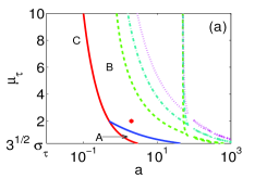
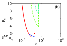
Figure 1: A selection of the bifurcation curves of the mean field model Eq. (2) in the parameter space of coupling strength $a$ and mean time delay $\mu_{\tau}$ for different values of the time delay standard deviation $\sigma_{\tau}=0.2$ (a) and 0.6 (b). In region A (a) the stationary state of the mean field is stable; this state corresponds to the ring state (see text) of the full swarm system Eq. (1). The swarm moves uniformly in region C (a), this ‘translating state’ disappears by merging with the stationary state along the curve $a\mu_{\tau}=1$ (red). The stationary state undergoes a first Hopf bifurcation along the curve above region A (a), making the mean field adopt a ‘rotating state’ in region B (a). The stationary state has an infinite series of higher order Hopf bifurcations; the first few members are shown in dashed curves (green, cyan and magenta). Comparing (a) and (b), we see how sensitive these additional Hopf curves are with respect to $\sigma_{\tau}$. The marker at $a=2$ and $\mu_{\tau}=2$ denotes the parameter values used for our numerical investigations. (Color online).

A mean field approximation of the swarm dynamics may be obtained by using coordinates relative to the center of mass $\mathbf{r}_{i}=\mathbf{R}+\delta\mathbf{r}_{i}$, for $i=1,2\ldots,N$, where $\mathbf{R}(t)=\frac{1}{N}\sum_{i=1}^{N}\mathbf{r}_{i}(t)$. Following [33], we use the following distributed delay equation to describe the mean field of the swarm:

$$\ddot{\mathbf{R}}= \left(1-|\dot{\mathbf{R}}|^{2}\right)\dot{\mathbf{R}}-a\left(\mathbf{\ R}(t)-\int_{0}^{\infty}\mathbf{R}(t-\tau)\rho(\tau)d\tau\right).$$ (2)

For Eq. (2) to be accurate, we require that $N$ be sufficiently large so that $\frac{1}{N(N-1)}\sum_{i=1}^{N}\mathop{\sum_{j=1}^{N}}_{i\neq j}\mathbf{R}(t-\tau_{ij})\approx\int_{0}^{\infty}\mathbf{R}(t-\tau)\rho(\tau)d\tau$ and that the swarm particles remain relatively close together. However, since the proximity of the particles is not controlled directly by any parameter, one must rely on numerical simulations of finite swarm populations to establish the parameter regimes where the approximation holds.

III Results

In the absence of noise, Eqs. (1) have been shown to possess a rich bifurcation structure, elucidated by the use of the mean field approximation Eq. (2) (Figure 1) [33]. In contrast to the mean field, the full system displays bistability of several coherent patterns. In particular, in wide portions of region B in Fig. 1a, Eqs. (1) possesses bistability of two different patterns: (i) a ‘ring state’, where the center of mass of the swarm is at rest and the agents rotate both clockwise and counterclockwise at a constant speed and radius $1/\sqrt{a}$; (ii) a ‘rotating state’, where the particles form a fairly dense clump and move along a circular arc at constant speed, with all velocity vectors approximately aligned. The initial alignment of the particle velocities and the width of the time delay distribution are instrumental in determining what pattern is adopted after the decay of transients. Specifically, decreasing initial velocity alignment and increasing width of the delay distribution results in a higher liklihood of convergence to the ring state.

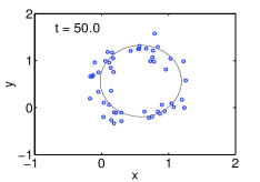
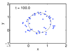
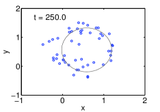
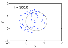
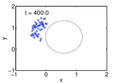
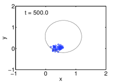
Figure 2: Snapshots of the swarm agents at different times, illustrating the transition from the ring state to the rotating state. Here $\sigma_{\tau}$=0.2 and $D=$0.23. The circle in the different panels is simply shown as a guide to the eye.

When noise is introduced, the combination of the coupling strength, the time delay and noise produces interesting pattern transitions due to the fluctuations of the agent’s alignment. Specifically, we find that when there is bistability of the ring and rotating state, there is a critical value of the noise intensity, $D_{crit}$, above which the swarm transitions from the ring state to the rotating state. In contrast, noise intensities below that critical value do not produce such a transition; that is, no such transition has been observed within the limits of our long-time numerical simulations. Figure 2 shows snapshots of the swarm, illustrating this transition. Here, and the rest of the simulations discussed below, the initial state of the particles is considered to be at rest and the particles are randomly distributed on the unit square. The new state of the swarm at each time step is found by updating the stochastic system (1) using Heun’s Method. In all simulations we assume the delays $\tau$ are uniformly distributed with a mean delay of $\mu_{\tau}$ and a standard deviation of $\sigma_{\tau}$. The noise is assumed to be Gaussian with intensity $D$. For all of our numerical studies, we use the values $N=50$, $a=2$ and $\mu_{\tau}=2$.

A remarkable fact is that noise intensities $D>D_{crit}$ produce a transition from a less coherent state into another with higher coherence. This is because the ring state is a disorganized state with both position and velocity vectors adopting wide probability distributions. In contrast, the rotating state is highly coherent, with particles having nearby locations (high density swarms) and almost perfect velocity alignment.

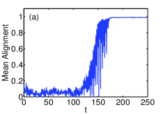
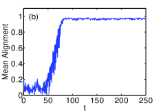
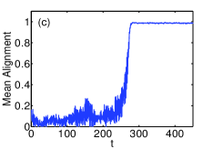
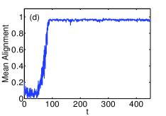
Figure 3: Time series showing the mean particle alignment as a function of time, for different parameter values. The top row has time delay standard deviation $\sigma_{\tau}=$0.2 and noise intensities $D=$0.25 (a) and 0.4 (b). The bottom row has time delay standard deviation $\sigma_{\tau}=$0.6 and noise intensities $D=$0.25 (c) and 0.4 (d). Please note the different scales on the abcissa axis.

In order to properly quantify the time required by the swarm to make this transition, we use a quantity called the mean alignment, which has been used in the past to describe the pattern adopted by the swarm as a whole [32]. This quantity is defined as follows. If the velocity of particle $j$ makes an angle $\theta_{j}$ with the velocity of the center of mass, then the mean alignment is simply the ensemble average of the cosines of all of the angles $\theta_{j}$, for $j=1,2\ldots N$. That is,

$$\textrm{Mean swarm alignment}=\frac{1}{N}\sum_{j=1}^{N}\cos\theta_{j}=\frac{1}{N}\sum_{j=1}^{N}\frac{\dot{\mathbf{r}}_{j}\cdot\dot{\mathbf{R}}}{|\dot{\mathbf{r}}_{j}||\dot{\mathbf{R}}|},$$ (3)

which ranges from -1 to 1. When all particles have perfectly aligned velocities, the mean alignment is equal to 1, regardless of their location in space or the magnitude of the individual particles’ speeds.

Figure 3 shows the mean particle alignment as a function of time, for different values of the noise intensity and the time delay standard deviation. The four panels show how the swarm starts with very low values of the mean alignment, since it initially adopts the ring state. After some dwell time in the ring state, the noise causes the swarm depart from that state and converge to the rotating state, where the mean alignment is almost 1.0. Once the agents begin to depart from the ring state, the transition time required to complete the transition is very short compared to the dwell time. For the simulations shown, the dwell time decreases with increasing noise intensity (Fig. 3a to 3b and Fig. 3c to 3d) and increases with increasing time delay standard deviation (Fig. 3a to 3c and Fig. 3b to 3d).

To better understand the onset of alignment due to noise, we probe different noise intensities for various choices of $\sigma_{\tau}$, with $\mu_{\tau}$ fixed, and then plot their asymptoptic mean alignment Figure 4. Each of the numerical experiments in Figure 4 was started in an initial state that, outside of the presence of noise, will stay indefinitely in the ring formation (unaligned). The simulation was run out to $t=2500$, in order to allow transients to pass, and to ensure we capture any transition between the two states. As reported in [32], we do see a critical value of the noise intensity $D$ at which the noise drives the particles into the highly aligned rotating state. Interestingly, as $\sigma_{\tau}$ is increased, the location of the $D_{crit}$ shifts so that a larger noise intensity is required to observe this transition. Thus, we observe a dependence of the critical noise threshold on the distribution width of the delays.

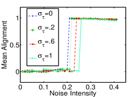
Figure 4: Asymptotic mean particle alignment as a function of the noise intensity parameter, $D$, and for different values of the time delay standard deviation $\sigma_{\tau}$. Each curve (labeling different values of the standard deviation of the time delay) has an extremely sharp transition that occurs at a critical value of the noise intensity $D_{crit}$ ($0.2<D_{crit}<0.25$). Below the transition point the swarm converges to the ring state and remains there for times as long as our simulations permit. In contrast, above the critical noise value, the swarm transitions to the more coherent, rotating sate.

Further, as observed in Fig. 3, increasing $\sigma_{\tau}$ also increases the amount of time the particles remain in the ring state before finally transitioning to the rotating state (assuming $D$ is large enough for such a transition to occur). To better understand this observation, we do single runs for various values of $\sigma_{\tau}$ and $D$. For each simulation, we monitor when a threshold value of the mean alignment is reached, and then record that time as the ‘dwell time’. While these dwell time values, shown in figure 5, record only single events, they do indicate that, generally speaking, below the threshold value $D<D_{crit}(\sigma_{\tau})$, we do not observe a transition out of the ring state, but for $D\geq D_{crit}(\sigma_{\tau})$, we observe that the dwell time is highest near the threshold, and then rapidly decreases as $D$ is increased. As one continues to increase $D$ even further, the rotating state will gradually become more disorganized until noise dominates the entire system.

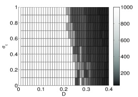
Figure 5: Dwelling time in the ring state, as a function of noise intensity, $D$, and the time delay standard deviation, $\sigma_{\tau}$. Below the $\sigma_{\tau}$-dependent, critical value of noise intensity, $D_{crit}$, the transition times diverge from the perspective of our long-time numerical simulations (white region). Above the value $D_{crit}$, the transition times become finite and accessible to computation from numerical simulations.

IV Discussion

We have considered the general problem of multi-agent swarms of particles where the communication is governed by a delay coupled potential field. In particular, we have considered the case where the delay coupling is fixed in time but randomly distributed from a chosen probability density. This corresponds to the fact that in many cases the delays in signal transmission and/or reception are caused by finite transmission times, processing and control delays, and the probability of dropped packets. Modeling the swarm as a globally coupled delay system, we have considered the role of temporal noise due to fluctuations from external forces which occur when the swarm is operating in a random field. In particular, we have considered parameters of the distributed delay system in which there exists bi-stability; i.e., there co-exists both a ring state and a rotating state.

For a given noise density and delay distribution, we have characterized the observation that a specific range of noise intensities forces a swarm from a disordered ring state, to a more ordered rotating state. By probing the effects of noise intensity along with the delay distribution width, we see a two parameter set which describes fluctuations which cause switching between disordered and ordered states. In particular, fluctuations due to sufficient noise intensities are observed to produce highly coherent and compact structures, which is clearly a non-intuitive result. We note once more that the patterns and the transitions between them, do not fundamentally change with the addition of small, local repulsive forces between particles. Stronger repulsion can, however, destabilize the coherent structures.

Understanding these types noise-induced transitions is key to preventing coherence collapse in delay-coupled autonomous systems, as well as formulating control strategies. In particular, the idea of a critical noise threshold which can serve to facilitate transitions between different dynamic patterns is very interesting and powerful, and understanding its dependence on the structure of delay-coupled systems is an area of ongoing interest.

We note that in the future, more work is required to understand the role of fluctuations on delay coupled systems. Towards this end, a general theory of switching for non-Gaussian noise is needed. In addition, more systematic numerical simulations will allow sufficient averaging to refine our understanding of the transitions discussed here. In addition, realistic networks of communication need to be considered beyond the globally coupled system modeled here.

V Acknowledgements

The authors gratefully acknowledge the Office of Naval Research for their support through ONR contract no. N0001412WX2003 and the Naval Research Laboratory 6.1 program contract no. N0001412WX30002. LMR and IBS are supported by Award Number R01GM090204 from the National Institute Of General Medical Sciences. The content is solely the responsibility of the authors and does not necessarily represent the official views of the National Institute Of General Medical Sciences or the National Institutes of Health. BSL is currently supported by a National Research Council fellowship.

References

- [1] E. Budrene and H. Berg, “Dynamics of formation of symmetrical patterns by chemotactic bacteria,” Nature, vol. 376, no. 6535, pp. 49–53, 1995.
- [2] J. Toner and Y. Tu, “Long-range order in a two-dimensional dynamical xy model: How birds fly together,” Phys. Rev. Lett., vol. 75, no. 23, pp. 4326–4329, 1995.
- [3] J. K. Parrish, “Complexity, pattern, and evolutionary trade-offs in animal aggregation,” Science, vol. 284, pp. 99–101, Apr 1999.
- [4] C. Topaz and A. Bertozzi, “Swarming patterns in a two-dimensional kinematic model for biological groups,” SIAM Journal on Applied Mathematics, vol. 65, no. 1, pp. 152–174, 2004.
- [5] D. Hebling and P. Molnar, “Social force model for pedestrian dynamics,” Phys. Rev. E., vol. 51, pp. 4282–4286, 1995.
- [6] F. D. C. Farrell, M. C. Marchetti, D. Marenduzzo, and J. Tailleur, “Pattern formation in self-propelled particles with density-dependent motility,” Phys. Rev. Lett., vol. 108, p. 248101, Jun 2012.
- [7] S. Mishra, K. Tunstrøm, I. D. Couzin, and C. Huepe, “Collective dynamics of self-propelled particles with variable speed,” Phys. Rev. E, vol. 86, p. 011901, Jul 2012.
- [8] C. Xue, E. O. Budrene, and H. G. Othmer, “Radial and spiral stream formation in Proteus mirabilis colonies,” PLoS Comput Biol, vol. 7, p. e1002332, 12 2011.
- [9] N. Leonard and E. Fiorelli, “Virtual leaders, artificial potentials and coordinated control of groups,” in Proc. of the 40th IEEE Conference on Decision and Control., vol. 3, pp. 2968–2973, 2002.
- [10] E. Justh and P. Krishnaprasad, “Steering laws and continuum models for planar formations,” in Proc. of the 42nd IEEE Conference on Decision and Control., vol. 4, pp. 3609–3614, 2004.
- [11] D. Morgan and I. B. Schwartz, “Dynamic coordinated control laws in multiple agent models,” Phys. Lett. A, vol. 340, no. 1-4, pp. 121–131, 2005.
- [12] Y.-L. Chuang, Y. R. Huang, M. R. D’Orsogna, and A. L. Bertozzi, “Multi-vehicle flocking: Scalability of cooperative control algorithms using pairwise potentials,” in Proc. of the 2007 IEEE International Conference on Robotics and Automation., pp. 2292–2299, 2007.
- [13] K. M. Lynch, P. Schwartz, I. B. Yang, and R. A. Freeman, “Decentralized environmental modeling by mobile sensor networks,” IEEE Trans. Robotics, vol. 24, no. 3, pp. 710–724, 2008.
- [14] C. Hsieh, Z. Jin, D. Marthaler, B. Nguyen, D. Tung, A. Bertozzi, and R. Murray, “Experimental validation of an algorithm for cooperative boundary tracking,” in Proc. of the 2005 American Control Conference., pp. 1078–1083, 2005.
- [15] I. Triandaf and I. B. Schwartz, “A collective motion algorithm for tracking time-dependent boundaries,” Mathematics and Computers in Simulation, vol. 70, pp. 187–202, 2005.
- [16] B. Lu, J. Oyekan, D. Gu, H. Hu, and H. F. G. Nia, “Mobile sensor networks for modelling environmental pollutant distribution,” Int. J. Sys. Sci., vol. 42, no. 9, SI, pp. 1491–1505, 2011.
- [17] T. Chung, J. Burdick, and R. Murray, “A decentralized motion coordination strategy for dynamic target tracking,” in Proc. 2006 Conference on International Robotics and Automation, pp. 2416–22, 2006.
- [18] A. Papachristodoulou and A. Jadbabaie, “Synchronization in oscillator networks with heterogeneous delays, switching topologies and nonlinear dynamics,” in Proc. of the 45th IEEE Conference on Decision and Control, pp. 4307 – 4312, 2007.
- [19] T. W. Mather and M. A. Hsieh, “Macroscopic modeling of stochastic deployment policies with time delays for robot ensembles,” Int. J. Robot Res., vol. 30, pp. 590–600, APR 2011.
- [20] A. Englert, S. Heiligenthal, W. Kinzel, and I. Kanter, “Synchronization of chaotic networks with time-delayed couplings: An analytic study,” Phys. Rev. E, vol. 83, APR 26 2011.
- [21] Z. Zuo, C. Yang, and Y. Wang, “A unified framework of exponential synchronization for complex networks with time-varying delays,” Phys. Lett. A, vol. 374, pp. 1989–1999, APR 19 2010.
- [22] K. Konishi, H. Kokame, and N. Hara, “Stabilization of a steady state in network oscillators by using diffusive connections with two long time delays,” Phys. Rev. E, vol. 81, JAN 2010.
- [23] A. Ahlborn and U. Parlitz, “Controlling spatiotemporal chaos using multiple delays,” Phys. Rev. E, vol. 75, JUN 2007.
- [24] D. Wu, S. Zhu, and X. Luo, “Cooperative effects of random time delays and small-world topologies on diversity-induced resonance,” EPL, vol. 86, JUN 2009.
- [25] A. C. Marti, M. Ponce C, and C. Masoller, “Chaotic maps coupled with random delays: Connectivity, topology, and network propensity for synchronization,” Physica A, vol. 371, pp. 104–107, NOV 1 2006.
- [26] T. Omi and S. Shinomoto, “Can distributed delays perfectly stabilize dynamical networks?,” Phys. Rev. E, vol. 77, APR 2008.
- [27] G. Q. Cai and Y. K. Lin, “Stochastic analysis of time-delayed ecosystems,” Phys. Rev. E, vol. 76, p. 041913, Oct 2007.
- [28] M. I. Dykman and I. B. Schwartz, “Large rare fluctuations in systems with delayed dissipation.” arXiv:1204.6519, 2012.
- [29] T. Vicsek, A. Czirók, E. Ben-Jacob, I. Cohen, and O. Shochet, “Novel type of phase transition in a system of self-driven particles,” Phys. Rev. Lett., vol. 75, no. 6, pp. 1226–1229, 1995.
- [30] U. Erdmann and W. Ebeling, “Noise-induced transition from translational to rotational motion of swarms,” Phys. Rev. E, vol. 71, no. 051904, 2005.
- [31] E. Forgoston and I. B. Schwartz, “Delay-induced instabilities in self-propelling swarms,” Phy. Rev. E, vol. 77, no. 035203(R), 2008. arXiv:0712.2950.
- [32] L. Mier-y Teran-Romero, E. Forgoston, and I. B. Schwartz, “Coherent pattern prediction in swarms of delay-coupled agents.” IEEE TRO, accepted. arXiv:1205.0195., 2011.
- [33] B. Lindley, L. Mier-y Teran, and I. B. Schwartz, “Randomly distributed delayed communication and coherent swarm patterns,” 2012 IEEE International Conference on Robotics and Automation (ICRA), pp. 4260-4265, 2012.
- [34] L. Mier-y Teran, B. Lindley, and I. B. Schwartz, ‘Statistical multi-moment bifurcations in random delay coupled swarms” arXiv:1205.2047 ., 2012.
- [35] A. S. Mikhailov and D. Zanette, “Noise-induced breakdown of coherent collective motion in swarms,” Phys. Rev. E, vol. 60, pp. 4571–4575, 1999.
- [36] M. D’Orsogna, Y. Chuang, A. Bertozzi, and L. Chayes, “Self-propelled particles with soft-core interactions: Patterns, stability, and collapse,” Phys. Rev. Lett., vol. 96, no. 104302, 2006.
- [37] J. Strefler, U. Erdmann, and L. Schimansky-Geier, “Swarming in three dimensions,” Phys. Rev. E, vol. 78, no. 031927, 2008.