Cosmological shock waves: clues to the formation history of haloes

Abstract

Shock waves developed during the formation and evolution of cosmic structures are key features encoding crucial information on the hierarchical formation of the Universe. We present the analysis of an Eulerian adaptive mesh refinement (AMR) hydrodynamical and N-body simulation in a $\Lambda$CDM cosmology especially focused on the study of cosmological shock waves. The combination of a shock-capturing algorithm together with the use of a halo finder allows us to study the morphological structures of the shock patterns, the statistical properties of shocked cells, and the correlations between the cosmological shock waves appearing at different scales and the properties of the haloes harbouring them. According to their localisation with respect to the population of haloes in the simulation, shocks can be split into two broad classes: internal weak shocks related with evolutionary events within haloes, and external strong shocks associated with large-scale events. The shocks segregation according with their characteristic sizes is also visible in the shock distribution function. This function contains information on the abundances and strength of the different shocks, and it can be fitted by a double power law with a break in the slope around a Mach number of 20. We introduce a generalised scaling relation that correlates the average Mach numbers within the virial radius of haloes and their virial masses. In this plane, Mach number - virial mass, two well-differentiated regimes appear. Haloes occupy different areas of such plane according to their early evolutionary histories: those haloes with a relatively quiet evolution have an almost constant Mach number independently of their masses, whereas haloes undergoing significant merger events very early in their evolution show a linear dependence with their masses. At high redshift, the distribution of haloes in this plane forms an L-like pattern that evolves with time bending the vertical branch towards the horizontal one. We prove that this behaviour is produced by haloes reaching low average Mach numbers as they evolve towards a virialised state. The analysis of the propagation speed and size of the shock waves developed around haloes could give some hints on the formation time and main features of the haloes. The possible future detection of all sort of cosmic shocks by the forthcoming telescopes, such as the SKA, could open a new window to indirectly unravel some of the main features of haloes and, therefore, the formation process of the cosmic structures.

1 Introduction

The cosmological shock waves develop as a consequence of the hierarchical formation of structures in the Universe and, therefore, they are crucial ingredients in a unified picture of the formation of cosmological structures. In a first phase, gravitational energy associated to the collapse of dark matter haloes corresponding to galaxy clusters and galaxies is transformed into internal energy of the intra cluster medium (ICM) and inter galactic medium (IGM) gaseous components. In the following phases, the evolution of those structures also produces mergers and accretion phenomena that modify the energetic balance of the gas through shock waves. Therefore, the shocks associated to cosmic structure formation and evolution encode information about the formation of the structures and their thermal impact on the gas.

The cosmological shocks can be broadly classified into two categories (e.g., Ryu et al., 2003): external and internal. External shocks surround filaments, sheets, and haloes, while internal shocks are located within the regions bound by external shocks and are created by flow motions correlated with structure formation and evolution. On large scales, the thermal history of galaxy clusters is dominated by the infall of material onto dark matter haloes and the conversion of gravitational energy into thermal energy of the gas. This process occurs through the heating of the gas via strong (external) accretion shocks surrounding galaxy clusters and filaments (e.g., Ryu et al., 2003; Miniati et al., 2001; Pfrommer et al., 2006). Inside collapsed structures, weaker (internal) shocks can be subdivided in three different classes: (i) accretion shocks caused by infalling gas in cosmic structures, (ii) merger shocks resulting from merging haloes, and (iii) random flow shocks inside nonlinear structures produced during hierarchical clustering. These internal shocks contribute to the virialization of haloes.

The role of shocks in cosmological structures has been studied from different complementary approaches. From the observational point of view, strong shocks usually develop in the external low-density regions of galaxy clusters where observable emission, such as X-ray emission, is weak. As a consequence, from an observational point of view, detecting shocks on large scales is still very challenging. Despite these difficulties, few large cosmic shocks have been positively detected by means of the so-called radio relics (e.g., Ensslin et al., 1998), commonly defined as elongated radio emission not associated with the cluster centre or an active cluster radio galaxy. These radio relics are found in $\sim 30$ clusters (e.g., Bagchi et al., 2006; Venturi et al., 2007; Bonafede et al., 2009; van Weeren et al., 2009). Peripheral radio relics on the outskirts of some massive clusters are the brightest of the cluster shock structures and are interpreted as externally propagating merger shocks that reach higher Mach numbers as they enter the low-density regions of the ICM. Concerning internal shocks, in a few cases, shocks driven by merging events have been observed with very low ($\approx 1.5-3$) Mach numbers (e.g., Markevitch, Sarazin & Vikhlinin, 1999; Markevitch et al., 2002; Markevitch & Vikhlinin, 2007).

From the theoretical point of view, several attempts to study shocks were done using semi-analytical approaches (Press & Schechter, 1974; Sheth & Tormen, 1999; Pavlidou & Fields, 2006; Fujita & Sarazin, 2001; Gabici & Blasi, 2003). However, the complexity of the considered scenario proved the use of numerical approaches as the most suited to study and characterise the shocks produced during the formation and evolution of cosmic structures. There have been numerical studies of shocks using both Eulerian, “single-grid” (e.g., Quilis, Ibá$\tilde{n}$ez & Sáez, 1998; Miniati et al., 2000; Ryu et al., 2003; Kang et al., 2007; Vazza, Brunetti & Gheller, 2009) and “AMR-grid” approaches (Skillman et al., 2008; Vazza et al., 2009, 2010), as well as SPH codes (e.g., Pfrommer et al., 2006; Pfrommer, Enßlin & Springel, 2008; Hoeft et al., 2008). Even when the debate about the benefits and drawbacks of different numerical techniques is still open (e.g., Agertz et al., 2007), the inherent shock-capturing properties of the Eulerian techniques based on Riemann solvers, able to deal with shocks by construction, seem to position this kind of tools as the recommended ones when tackling shock related processes. In this regard, Vazza et al. (2011) presented a numerical study of non-radiative cosmological simulations, at various resolutions and performed with different cosmological codes, comparing the properties of thermal gas and shock waves in large scale structures. Even when the bulk of thermal and shock properties were reasonably in agreement between the Eulerian and the SPH codes, they also reported some significant differences between them like, for instance, differences of large factors ($\sim 10-100$) in the values of average Mach numbers and shock thermal energy flux in the most rarefied regions of the simulations, significantly different phase diagrams of shocked cells in grid codes compared to SPH, or sizable differences in the morphologies of accretion shocks between grid and SPH methods.

Pioneering attempts to characterise shock waves in cosmological simulations were carried out by Quilis, Ibá$\tilde{n}$ez & Sáez (1998) and Miniati et al. (2000). They employed fix grid Eulerian simulations and shock-detecting schemes based on jumps in the main thermodynamical quantities. Later works adopted more refined shock-detecting algorithms and were more focused onto the distribution of energy dissipated at shocks (e.g., Miniati, 2002; Ryu et al., 2003; Pfrommer et al., 2006; Vazza, Brunetti & Gheller, 2009). Despite the important advances, in the first works using uniform grid-based codes, it was not possible to cover the spatial resolutions required to describe both the complex flows within haloes and their coupling to large-scale structures. Further improvement has been reached by Skillman et al. (2008) using a shock-detecting scheme looking for shocks in the direction of the temperature gradients on an AMR grid.

These numerical simulations have begun to reveal a rich network of shock structures throughout the ICM (e.g., Miniati et al., 2001b; Ryu et al., 2003; Pfrommer, Enßlin & Springel, 2008; Battaglia et al., 2009; Skillman et al., 2010; Vazza et al., 2010). However, in spite of all previous works, the identification and characterisation of shocks is still challenging due to the complex dynamics involved in the formation and evolution of cosmological structures and to the large dynamical range needed to describe all the scales involved by shocks.

Our purpose in the present paper is to pursue the analyses of the main properties of the shock waves developed during the evolution of a high resolution hydrodynamical and N-body simulation of a large cosmological volume performed with an AMR cosmological code. In addition, we will put especial emphasis in analysing the existing connection between the cosmological shock waves and the population of haloes. In order to do so, we have developed a numerical algorithm able of detecting and characterising shocks in 3-D AMR simulations. The use of AMR hydro codes turns out to be crucial so as to obtain good dynamical ranges with an advanced hydrodynamical algorithm that is able to capture shocks very accurately.

The paper is organised as follows. In Section 2, we present the technical details describing the simulation and the shock-finding algorithm. The results of the analysis of the simulation are presented in Section 3. Finally, in Section 4, we summarise and discuss our results.

2 Detecting shock waves

2.1 Simulation details

The simulation used in this paper was performed with the cosmological code MASCLET (Quilis, 2004). This code couples an Eulerian approach based on the so-called high-resolution shock-capturing techniques (e.g., LeVeque, 1992) for describing the gaseous component, with a multigrid particle mesh N-body scheme for evolving the collisionless components (dark matter and stars). Gas, dark matter, and stars are coupled by the gravity solver. Both schemes benefit of using an adaptive mesh refinement (AMR) strategy, which permits to gain spatial and temporal resolution.

The numerical simulation was run assuming a spatially flat $\Lambda CDM$ cosmology, with the following cosmological parameters: matter density parameter, $\Omega_{m}=0.25$; cosmological constant, $\Omega_{\Lambda}=\Lambda/{3H_{o}^{2}}=0.75$; baryon density parameter, $\Omega_{b}=0.045$; reduced Hubble constant, $h=H_{o}/100km\,s^{-1}\,Mpc^{-1}=0.73$; power spectrum index, $n_{s}=1$; and power spectrum normalisation, $\sigma_{8}=0.8$.

The initial conditions were set up at $z=50$, using a CDM transfer function from Eisenstein & Hu (1998), for a cube of comoving side length $64\,Mpc$ discretised in $512^{3}$ cubical cells.

A first level of refinement (level $l=1$) for the AMR scheme was set up from the initial conditions by selecting regions satisfying certain refining criteria, when evolved – until non-linear phase– using the Zel’dovich approximation. The dark matter component in the initial refined region was sampled with dark matter particles eight times lighter than those used in regions covered only by the coarse grid (level $l=0$). During the evolution, regions on the different grids are refined based on the local baryonic and dark matter densities. Thus, a cell is refined, independently of the refinement level, if its dark matter (gaseous) mass is larger than $4.74\times 10^{8}M_{\odot}\,(1.04\times 10^{8}M_{\odot})$. This is equivalent to refine the cell if its density increases a factor of eight. The ratio between the cell sizes for a given level ($l+1$) and its parent level ($l$) is, in our AMR implementation, $\Delta x_{l+1}/\Delta x_{l}=1/2$. This is a compromise value between the gain in resolution and possible numerical instabilities.

The simulation presented in this paper uses a maximum of six levels ($l=6$) of refinement, which gives a peak physical spatial resolution of $\sim 4\,kpc$. For the dark matter we consider two particles species which correspond to the particles on the coarse grid and the particles within the first level of refinement at the initial conditions. The best mass resolution is $\sim 2.7\times 10^{8}\,h^{-1}\,M_{\odot}$, equivalent to distribute $512^{3}$ particles in the whole box.

Our simulation includes cooling and heating processes which take into account inverse Compton and free-free cooling, UV heating (Haart & Madau, 1996) at $z\sim 6$, atomic and molecular cooling for a primordial gas, and star formation. In order to compute the abundances of each species ($H,\,He,\,H^{+},\,He^{+},\,He^{++}$), we assume that the gas is optically thin and in ionization equilibrium, but not in thermal equilibrium (Katz, Weinberg & Hernquist, 1996; Theuns et al., 1998). The tabulated cooling rates were taken from Sutherland & Dopita (1993) assuming a constant metallicity 0.3 relative to solar. The cooling curve was truncated below temperatures of $10^{4}\,K$. The cooling and heating were included in the energy equation (see Eq. 3 in Quilis, 2004) as extra source terms.

The star formation is introduced in the MASCLET code following the ideas of Yepes et al. (1997) and Springel & Hernquist (2003). In our particular implementation, we assume that cold gas in a cell is transformed into star particles on a characteristic time scale $t_{*}$ according to $\dot{\rho_{*}}=-\dot{\rho}=(1-\beta)\,{\rho}/{t_{*}(\rho)}$ where $\rho$ and $\rho_{*}$ are the gas and star densities, respectively. The parameter $\beta$ stands for the mass fraction of massive stars ($>8\,M_{\odot}$) that explode as supernovae, and therefore return to the gas component in the cells. We adopt $\beta=0.1$, a value compatible with a Salpeter IMF. For the characteristic star formation time, we make the common assumption $t_{*}(\rho)=t^{*}_{o}(\rho/\rho_{{}_{th}})^{-1/2}$, equivalent to $\dot{\rho}_{*}=\rho^{1.5}/t^{*}_{o}$ (Kennicutt, 1998). In this way, we introduce a dependence on the local dynamical time of the gas and two parameters, the density threshold for star formation ($\rho_{{}_{th}}$) and the corresponding characteristic time scale ($t^{*}_{0}$). In our simulation, we take $t^{*}_{0}=2\,Gyr$ and $\rho_{{}_{th}}=2\times 10^{-25}\,g\,cm^{-3}$. From the energetic point of view, we consider that each supernova dumps in the original cell $10^{51}\,erg$ of thermal energy.

In the practical implementation, we assume that star formation occurs once every global time step, $\Delta t_{l=0}$, and only in the cells at the highest level of refinement. Those cells at this level of refinement, where the gas temperature drops below $T<2\times 10^{4}\,K$, the divergence of the velocity of the gas is $\nabla\cdot{\bf v}<0$, and the gas density is $\rho>\rho_{{}_{th}}=2\times 10^{-25}\,g\,cm^{-3}$, are suitable to form stars. In these cells, collisionless star particles with mass $m_{*}=\dot{\rho}_{*}\Delta t_{l=0}\Delta x_{l}^{3}$ are formed. In order to avoid sudden changes in the gas density, an extra condition restricts the mass of the star particles to be $m_{*}={\rm min}(m_{*},\frac{2}{3}m_{gas})$, where $m_{gas}$ is the total gas mass in the considered cell.

According with the previously described scheme for the star formation in our simulations, we include only one simple case of feedback, that is, the contribution in mass and energy from type II supernovae. No feedback from active galactic nucleus (AGN) or type Ia supernovae are considered. Although this point could be improved, how to model AGN feedback in cosmological simulations is still a matter of discussion (e.g., Fabjan et al., 2010). Besides, we do not expect a dramatic change in our results linked with the inclusion or not of feedback, since the formation and evolution of the cosmological shock waves are supposed to be mainly driven by the assembly of cosmic structures and, therefore, gravity should be the main ingredient to model.

A final technical consideration concerning the numerical resolution of the simulation must be done. We have not performed any resolution test and assume that our numerical resolution is adequate to study the processes related with shocks. We base our assumption in the work by Vazza et al. (2011), where authors compare the properties of shocks using different cosmological codes. We must point out that our numerical resolution – in cell size and particles masses – is much better than in all the simulations considered in Vazza et al. (2011) (see Table 1 of this reference), where the authors conclude that a very good convergence, better than a $\sim 10$ per cent level, in the most important shock statistics is expected for spatial resolutions of $\sim 50-100$ kpc, which are above than our best resolution.

2.2 Basic relations

Shocks produce irreversible changes in the gas of the cosmic structures. As a consequence, the formation of a shock in a cosmological volume produces a jump in all the thermodynamical quantities. If we assume that the pre-shocked medium is at rest and in thermal and pressure equilibrium, the pre-shock and post-shock values for any of the hydrodynamical variables are unambiguously related to the shock Mach number, $\mathcal{M}$. The Mach number, which characterises the strength of a shock, is given by

$$\mathcal{M}=v_{s}/c_{s},$$ (1)

where $v_{s}$ is the shock speed and $c_{s}$ is the sound speed ahead of the shock.

All the information needed to evaluate $\mathcal{M}$ is contained in the Rankine-Hugoniot jump conditions. If the adiabatic index is set to $\gamma=5/3$ we obtain, for the density ($\rho$), the temperature (T), and the entropy ($S=T/\rho^{\gamma-1}$), the well-known relations (e.g., Landau & Lifshitz, 1966):

$$\frac{\rho_{2}}{\rho_{1}}=\frac{4\mathcal{M}^{2}}{\mathcal{M}^{2}+3}$$ (2)

$$\frac{T_{2}}{T_{1}}=\frac{(5\mathcal{M}^{2}-1)(\mathcal{M}^{2}+3)}{16\mathcal{M}^{2}}$$ (3)

$$\frac{S_{2}}{S_{1}}=\frac{(5\mathcal{M}^{2}-1)(\mathcal{M}^{2}+3)}{16\mathcal{M}^{2}}(\frac{\mathcal{M}^{2}+3}{4\mathcal{M}^{2}})^{2/3}$$ (4)

with indices $1,2$ referring to pre- and post-shock quantities, respectively.

The Mach number can be obtained from the jumps in any of the hydrodynamical variables (Eqs. 2–4) or from a combination of them. In the case of relatively large Mach numbers, since the value of the density jump saturates at $\rho_{2}/\rho_{1}=4$ (Eq. 2), strong shocks cannot be detected from density jumps. As a consequence, the most effective methods to measure $\mathcal{M}$ are those considering temperature and entropy jumps.

2.3 Shock-finding algorithm

Any shock-finding method relies on accurately identifying and quantifying the strength of shocks. Although, during the simulations using an Eulerian approach, the shocks are automatically detected by the Riemann solver within the hydrodynamical routine, the analysis of these shocks requires additional considerations.

Recent works on algorithms to find and track shocks in grid simulations have stablished two procedures. Both methods require a previous step to mark the cells which are involved in a shock at the time corresponding to the analysed output. Once the shocked cells have been identified, the two methods differ in how to define the shocks. The first method (e.g., Vazza, Brunetti & Gheller, 2009) relies on following temperature or velocity jumps across the previously tagged shocked cells along the different coordinate axes. We define this method as the coordiante or directional-splitting method. According with Vazza, Brunetti & Gheller (2009), the results seem to be quite insensitive to the use of temperature or velocity jumps, with minor differences in the most rarefied environments. This kind of methods has a minor drawback when examining shocks that do not propagate along the coordinate axes. The second group of methods to find shocks use the local temperature gradient to figure out the direction of the shock propagation (e.g., Skillman et al., 2008). These methods would be more precise when dealing with complex flows or weak shocks. So as to minimise a possible smearing of the shocks produced by the coordinate-splitting or other uncontrolled numerical effects, the so-called coordinate-splitting methods define the final Mach number as the average of the Mach numbers along each coordinate axis. With this implementation, the differences between schemes based on a precise estimate of the direction of the shock propagation and others based on the directional-splitting are not expected to be significative.

Our shock-finding algorithm is based on temperature jumps and, therefore, comparable to the method in Vazza, Brunetti & Gheller (2009). Thus, the main steps of the shock-finding algorithm used in this paper are the following:

1. All cells within the computational volume are classified as tentative shocked or not shocked. A cell is labelled as tentative shocked if the fluid inside the cell meets the following requirements:

   $$\nabla\cdot{\bf v}<0$$ (5)

   $$\nabla T\cdot\nabla S>0$$ (6)

   where ${\bf v}$, $T$ and $S$ are, respectively, the velocity field, the temperature and the entropy of the fluid (gas) within the cell.

2. Among all the tentative shocked cells, the cell where $\nabla\cdot{\bf v}$ is minimum is flagged as the first shocked cell.

3. The sense of shock propagation with respect to the computational grid is computed by moving outwards from the previously identified shocked cell along each of the three coordinate axes. This extension is done meanwhile there are tentative shocked cells and the temperature and the density in these tentative shocked cells satisfy that $T_{2}>T_{1}$ and $\rho_{2}>\rho_{1}$. The subscripts 1 and 2 refer to the tentative shocked cells ahead and behind of the central shock cell in the shock reference frame, respectively. The shock discontinuities caught in the simulations by this method are typically spread over a few cells.

4. Once the furthest shocked cell ahead and behind of the central cell of the shock – that we denote as the pre- and post-shock cells – in each coordinated direction are found, the temperatures $T_{1}$ (pre-shock) and $T_{2}$ (post-shock) of these cells are taken and three different Mach numbers (one for each direction) are calculated from Eq. 3.

5. The strength of the shock is computed by combining the Mach numbers measured along the three coordinate axes: $\mathcal{M}=(\mathcal{M}_{x}^{2}+\mathcal{M}_{y}^{2}+\mathcal{M}_{z}^{2})^{1/2}$, which minimises projection effects in case of diagonal shocks (e.g., Vazza, Brunetti & Gheller, 2009).

6. The shocked cell drops out of the list of the tentative shocked cells, and the process is iteratively repeated focusing on the cell with minimum $\nabla\cdot{\bf v}$ among the remaining tentative shocked cells.

The whole procedure identifies all the shocked cells within the computational box and obtains their Mach number. The assembly of all these shocked cells defines the characteristic shock surfaces associated to shock waves.

When this procedure is applied to an AMR simulation, the analysis is carried out in a hierarchical fashion, first on the most highly refined grids, moving down to progressively coarser levels of resolution. Given that this procedure is applied, independently, at each level of refinement of the simulation, the algorithm is able to find, in a natural way, shock waves related to different spatial scales provided by the simulation itself. Although this is a very useful and interesting feature of our approach, the use of an AMR grid makes the process more complicated compared with a fix grid approach, especially when shocks extend over several subgrids at different levels. In this case, the algorithm goes on looking for the boundaries of the shock wave on the parent subgrid – in a lower level of refinement – that contains the original subgrid on which the shock was originally identified. This mechanism can be applied recursively on several levels if needed.

In all the analysis performed in following sections of this paper, in order to avoid noisy shock patterns with very low Mach numbers, we have considered a Mach number minimum threshold equal to $1.3$.

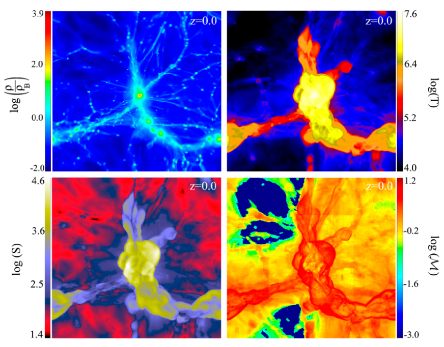
Figure 1: Large-scale distribution of several quantities at $z=0$. Each two-dimensional panel is $64$ Mpc side length. All quantities are integrated along a slice of thickness $L=10$ Mpc according with $q_{i}=\frac{1}{L}\int{qdx}$ where $q$ is a generic quantity to be projected and $q_{i}$ is the final plotted variable. The panels show: the integrated gas overdensity, $\rho/\rho_{{}_{B}}$, being $\rho_{{}_{B}}$ the background density (upper left), the integrated gas temperature in K (upper right), the integrated gas entropy in $keV\,cm^{2}$ (lower left) and the integrated Mach number (lower right). Different palettes have been used in order to highlight the particular features of each panel.

3 Results

3.1 Distribution of large-scale shocks

Shocks fill the simulated volume in a very complex pattern (e.g., Miniati et al., 2000; Ryu et al., 2003). Figure 1 illustrates typical structures found in large-scale cosmological simulations. The different two-dimensional panels ($64$ Mpc side length) represent the following integrated quantities along slices of $10$ Mpc thickness at $z=0$: the gas overdensity (upper left), the gas temperature (upper right), the gas entropy (lower left) and the Mach number (lower right). All the panels show the logarithm of the different quantities. The four projections are centred at the position of the largest cluster in the simulation ($M_{vir}\sim 8.0\times 10^{14}\,M_{\odot}$ and $R_{vir}\sim 2.4$ Mpc) which is almost at the centre of the box.

The panel presenting the gas overdensity in Fig. 1 shows the common picture of galaxy clusters connected through filaments. The shock waves, if existing, are not appreciable in this picture. The panel displaying the gas temperature clearly shows high temperature regions, where the gas has been heated up by shock moving outwards from the centre of the structure, and low temperature spots associated to regions where the gas cooled down during the cosmic evolution. The temperature plot gives a first preliminary idea of the regions which have been shocked. The entropy panel, as it would be expected, is a step forward highlighting the complex structure of shocks. In this particular panel, the boundaries of high temperature regions appear as high entropy zones indicating the presence of a shock or strong gradient. For completeness, the last panel shows the Mach number associated to the studied region. Now, the complex structure of shocks is clearly visible, showing a remarkable correlation with the entropy panel, although much sharper in this case. The Mach number map also allows to distinguish between high-Mach number shocks, wrapping the larger structures, and the low-Mach number shocks associated with internal small scale structures.

Figure 2: Left: Volume fraction occupied by shocked cells in the simulation as a function of redshift. Right: mean volume-weighted Mach number as a function of redshift.

The cosmic evolution of shock strengths encodes a valuable information about the thermal history of the baryonic component of the Universe. In Fig. 2, the filling volume factor of shocks – that is, the fraction of the computational volume occupied by shocked cells – is plotted versus redshift evolution (left panel), whereas the right panel shows the volume-weighted average Mach number for the same time evolution. A warning notice must be done at this point because, as already mentioned in Sec. 2.1, a resolution test has not been performed. Therefore, these results could be affected by resolution effects.

Early evolution ($z\gtrsim 6$) of the shocked volume evidences a non-negligible fraction of the computational box involved in shocks ($\sim 27\%$). This quantity increases towards its maximum at $z\sim 5$ when a step decline of the filling factor of shocks starts. The explanation of such behaviour is associated with huge amounts of gas falling into the potential wells created by cosmic structures – at different scales – at the beginning of their non-linear evolution. As the gas flows have relatively low densities and moderate velocities, they can easily reach supersonic regimes. Therefore, they can occupy an important volume of the simulated region. However, as it is shown in the right panel, these are weak shocks characterised by low volume-weighted Mach numbers.

As the non-linear evolution of cosmic structures continues, the number of collapsing regions increases, as well as the densities and velocities of the gas flows falling into such structures. The combination of these factors produces a maximum of the shocked volume and the shock strength around $z\sim 5$.

After this time two different trends appear depending on whether we look at the shocked volume or at the average shock strength. The first one continuously declines mainly due to the fact that structures start to collapse and to form bound haloes where the gas component is locked up and, therefore, the sizes of regions where shocks can appear get smaller as the time evolution goes on. On the other hand, the average shock strength shows the same behaviour immediately after its maximum but it changes its derivate around $z\sim 2$. The reason of this behaviour is strongly correlated with the increase of the merging rate among the already formed haloes of different masses and sizes. The final fraction of the simulated shocked volume reaches a value of $\sim 20\%$ at $z=0$.

This result on the temporal evolution of the fraction of the computational volume occupied by shocked cells seems to be in broad agreement with the results shown in Vazza, Brunetti & Gheller (2009) who obtained that the fraction of the simulated volume being shocked goes from roughly $30\%$ at high redshift ($z\geq 6$) down to $\sim 15\%$ at $z=0$.

A crucial tool in the study of cosmic structures is the mass distribution function of the different objects in the Universe. Following a similar approach to the mass function, we study the shocks distribution function (from now on SDF), defined as the variation of the number of shocked cells (volume-weighted) as a function of the Mach number. In Fig. 3 the differential SDF at $z=0$ is plotted – in logarithmic scale – to show the distribution of shocks in the simulated volume.

Figure 3: Shocks distribution function (SDF) at $z=0$ as a function of their Mach number in logarithmic bins.

The most remarkable feature of the SDF is the presence of two clearly differentiated regimes with different slopes. The first regime corresponds to low Mach numbers which are much more abundant. The second regime is steeper than the previous one and stands for strong shocks with higher Mach numbers which are the most rare in the studied volume. The transition between the two regimes takes place around $\mathcal{M}\sim 20$. This value for $\mathcal{M}$, as it will be discussed in the next sections, turns out to be a crucial number separating the internal shocks – located within the virial radius of the structures – and the external shocks at outer regions. The two different regions of the SDF can be fitted by power laws of the form $dN(\mathcal{M})/d\mathcal{M}\propto\mathcal{M}^{\alpha}$. Thus, for low Mach numbers (up to $\simeq 20$) we obtain a slope of $\alpha\simeq-1.7$, whereas for stronger shocks a steeper relation, $\alpha\simeq-4.1$, is found. Previous works already proved that the bulk of shocks in the universe is dominated by relatively weak shocks $(\mathcal{M}\leq 2)$, but there is also a population of stronger shocks located in the external regions of haloes where structures are not completely virialised (e.g., Ryu et al., 2003; Pfrommer et al., 2006; Vazza, Brunetti & Gheller, 2009).

We have also followed the time evolution of the SDF at several redshifts, finding very similar trends at all the epochs. The most relevant difference between the distributions obtained at different times is found at the high-Mach end of the relation, which slowly moves down to lower values when the redshift decreases. Only when quite high redshifts ($z\geq 6$) are reached, an important change in the shape of the distribution is appreciated although, probably, the information provided by the SDF at such high redshift is not relevant due to the early stage of evolution of the cosmic structures.

3.2 Shock waves and cosmic structures

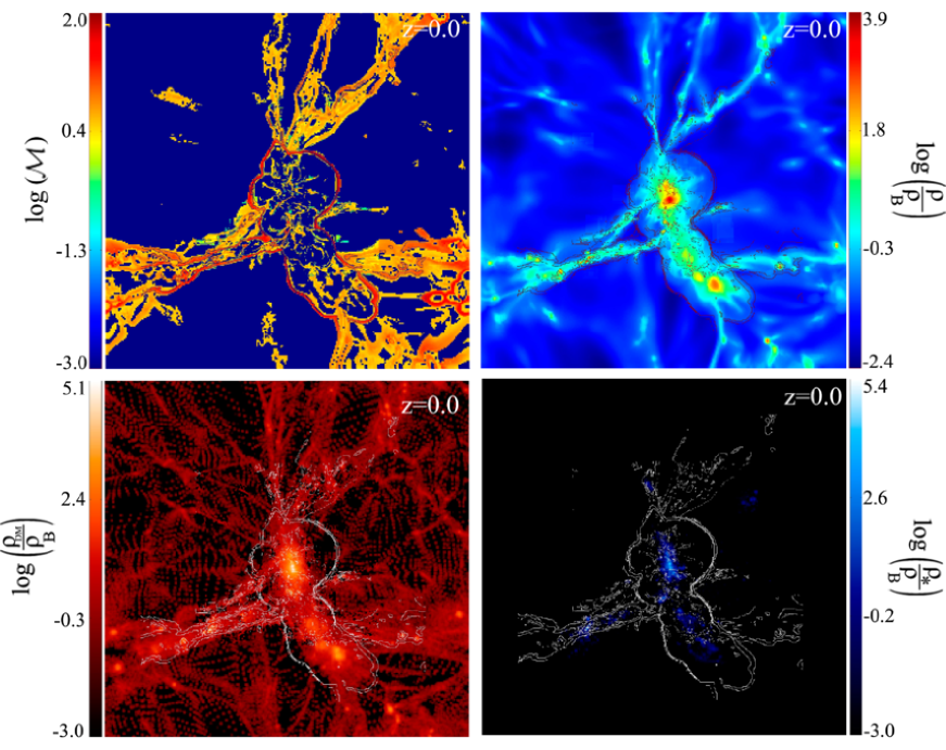
Figure 4: Distributions of Mach number compared with dark matter $(\rho_{DM}/\rho_{{}_{B}})$ , gas $(\rho/\rho_{{}_{B}})$ and stellar $(\rho_{*}/\rho_{{}_{B}})$ overdensities at $z=0$. Each panel is a thin slice of $0.2$ Mpc thickness and $64$ Mpc side length. They show the Mach number distribution (upper left) and the gas, dark matter and stellar overdensities (upper right, lower left, and lower right panels, respectively). In all the panels, the contours of the shock waves with high Mach numbers are overplotted.

Cosmological shocks derived from the formation and evolution of cosmic structures have to present some correlations with the main features of the distribution of such structures. In order to deepen in this connection, in the present Section we discuss the correlation between the distribution of cosmological shock waves and the halo population (galaxies and galaxy clusters).

The first analysis one can think about is to compare the shock pattern with the density distribution of the different components forming the haloes in the simulation. Thus, Fig. 4 shows a 2-D projection along the z axis of the Mach number distribution (upper left panel) to compare with the gas $(\rho/\rho_{{}_{B}})$, dark matter $(\rho_{DM}/\rho_{{}_{B}})$ and stellar $(\rho_{*}/\rho_{{}_{B}})$ overdensities (upper right, lower left, and lower right panels, respectively) at $z=0$. Each panel represents a thin slice of $0.2$ Mpc thickness and $64$ Mpc side length centred at the position of the most massive halo found in the computational box (the same than in Fig. 1). All the plotted quantities are in logarithmic scale. In all these panels, the contours of the strong shock waves – with high Mach numbers ($\mathcal{M}>20$) – are overplotted.

From Fig. 4 we can infer, as it was expected, that the shock pattern perfectly traces the cosmic web (e.g., Miniati et al., 2000). Nevertheless, this shock pattern has two clearly separated regimes. The first of these regimes gathers the high $\mathcal{M}$ shocks – overplotted as contour lines in Fig. 4 – that wrap filaments, sheets, and haloes. As these shocks are located out of the virial radius of the structures, they are classified as external shocks. These shocks have quasi-spherical geometries and can be located at distances of several virial radius from the centre of the structure where they were created (e.g., Vazza, Brunetti & Gheller, 2009). In general, such external shocks are the evolved state of the accretion shocks formed during the collapse of haloes. During their movement outwards from the halo centre, these accretion shocks interact among them creating, therefore, a more complex pattern.

Although for the sake of clarity the low-Mach number shocks are not plotted in Fig. 4, moving inwards the virial radius of haloes, more irregular and weaker shocks ($\mathcal{M}\leq 5$) are formed, in line with results from previous studies (e.g., Vazza, Brunetti & Gheller, 2009). This second regime corresponds to the internal shocks which are mainly associated to random flow motions and merger events within the haloes.

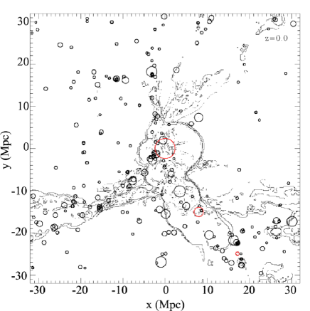
Figure 5: Distribution of dark matter haloes together with shock waves at $z=0$. The solid lines represent six contour levels of the higher-Mach number shock waves. This contour has been computed for a slice of the simulated box of $0.2$ Mpc depth and $64$ Mpc side length centred at the location of the most massive halo. Circles stand for all the found haloes in the computational box with masses larger than $\geq 10^{12}\,M_{\odot}$. We point out in red those haloes whose positions fit in the considered slice. The size of the circles represent the virial radius of the haloes.

In order to reinforce the previous idea, in Fig. 5 we compare the distribution of shock waves with high Mach numbers (given by the contour lines) with the spatial distribution of the dark matter haloes found in the simulation at $z=0$. This figure shows the same slice than in Fig. 4. The represented dark matter haloes have been identified with the ASOHF halo finder (Planelles & Quilis, 2010). Only objects with virial masses larger than $10^{12}\,M_{\odot}$ are considered. The total sample consists of $\sim$ 260 haloes at $z\sim 0$ within a range of masses between $1.0\times 10^{12}\,M_{\odot}$ and $8.0\times 10^{14}\,M_{\odot}$. The dark matter haloes are plotted as circles whose sizes represent their virial radius. Those haloes whose position perfectly fits in the analysed slice are drawn in red. It is clearly visible how the complex pattern of strong shocks – produced by the hierarchical evolution of the proto-haloes – surrounds the galaxy cluster (large red circle) from which these shocks stem from.

3.3 The Mach number scaling relation

The scaling relations are powerful tools in the understanding of the processes sculpting the formation and evolution of galaxy clusters and groups. The common way to use the scaling relations consists in plotting, for a given characteristic radius, the cluster mass against the temperature, the entropy, or the X-ray luminosity.

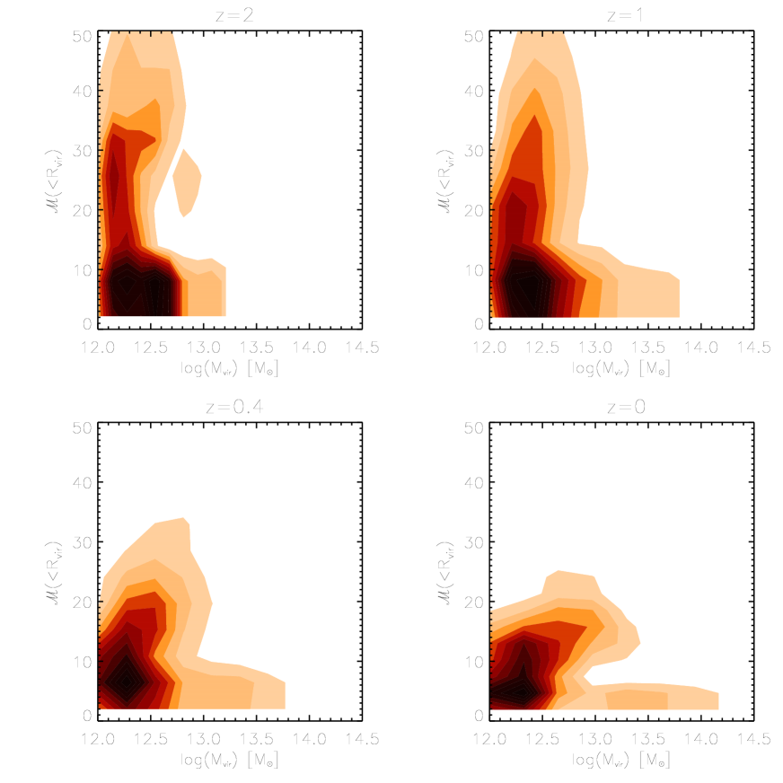
Figure 6: Halo distribution in the Mach number - virial mass plane. Results at $z\simeq 2,1,0.4$, and 0, are shown. The shaded regions have been computed by binning individual haloes into a two-dimensional grid in the plane $\mathcal{M}-M_{vir}$. Six contour lines equally spaced are plotted to highlight the two-dimensional distributions.

Starting from this idea, we generalize its fundamental concept and we introduce what we call the Mach number scaling relation. In order to build this relation we compute an average volume-weighted Mach number for each halo in our sample with $M_{vir}>10^{12}\,M_{\odot}$. This volume-weighted Mach number is computed within the virial radius of each halo and, therefore, it represents a virial Mach number. After that, we bin individual haloes into a two-dimensional grid of Mach number versus virial mass in order to have information on the number of haloes within a certain range of Mach numbers and viral masses. The obtained scaling relation is displayed in Fig. 6 in which we show different contour lines in order to highlight the shape of the 2-D distribution. Four different epochs corresponding to $z\simeq 2,1,0.4$, and 0, are shown. The sample of haloes with $M_{vir}>10^{12}\,M_{\odot}$ at these epochs ranges from $\sim 160$ haloes at $z\simeq 2$ to $\sim 260$ at $z=0$.

The analysis of Fig. 6 revels some striking features. Let us focus first on the analysis of the distribution at $z=0$ (lower right panel), where there are two well-differentiated trends. On the one hand, there is an almost constant region for low Mach numbers ($\mathcal{M}\lesssim 5$) which seems to be no-dependant on the mass of the haloes. On the other hand, a steeper trend along all the range of Mach numbers seems to be correlated with halo masses.

Our explanation for this distribution is that the first trend is occupied by haloes which started their evolution in a relatively smooth way, with no mergers or a few minor mergers. The shocks within the virial radius producing the average Mach numbers associated with these haloes are related with smooth accretion flows of gas falling into the objects during this quiescence evolution. Therefore, haloes that have been quietly set up since early phases of their evolution have low $\mathcal{M}$ an tend to be located at the bottom of the plane $\mathcal{M}-M_{vir}$ independently of their virial masses.

Complementary, haloes that initially were involved in merger events and in active phases of their evolution suffer violent events that produce stronger shocks compared with those in the previous region. In this branch of the $\mathcal{M}-M_{vir}$ plot, there is a strong dependence on the virial masses of haloes.

Therefore, the evolutionary history of each halo explains the bimodal segregation shown in Fig. 6, which is also observed through the temporal evolution. At early epochs, corresponding to the formation time of large galaxies and small groups of galaxies ($z\sim\,2$), an L-like pattern in the plane $\mathcal{M}-M_{vir}$ appears. These times correspond to highly non-linear epochs of the evolution of the haloes, with high rates of merger events and interaction among the structures at different spatial and mass scales. When advancing in time, the initial L-pattern trend progressively bends over to higher masses – corresponding to big galactic haloes and galaxy clusters – but lower Mach numbers, reaching the bimodal distribution, previously discussed, at $z\sim 0$.

In order to understand this behaviour, we have followed the global evolution of individual haloes looking at their overall drifts along the plane $\mathcal{M}-M_{vir}$. We have studied this evolution for the 22 more massive haloes in the simulation which, indeed, are the best numerically resolved. The haloes in this subsample evolve according to two different behaviours. Roughly the $50\%$ of this subsample of haloes begin, at high redshift, with a relatively high Mach number and evolve to progressively lower Mach numbers while increasing their mass. The remaining percentage of haloes depart from low-Mach number states ($\mathcal{M}<5$) and tend to move, during their evolution, almost parallel to the x-axis while augmenting their masses. Since our sample of haloes is far from being statistically complete we can not make a robust conclusion. However, our hypothesis to explain this behaviour is that the evolution of haloes along the plane $\mathcal{M}-M_{vir}$ is intimately related with their dynamical history. Like a gross trend, those haloes suffering important merger events (major mergers) early in their evolution only can evolve towards lower Mach numbers while reaching an equilibrium state producing, therefore, the decline of the initial L-like pattern into the flatter final distribution. On the other hand, haloes with a relatively quiet beginning show very low initial Mach numbers and evolve without significant changes in their virial Mach number and, consequently, they move almost parallel to the $M_{vir}$-axis while increasing their mass.

Let us point out that this general behaviour is not in contradiction with previous studies. Once haloes, due to their early evolution, are initially placed in the $\mathcal{M}-M_{vir}$ plane, shocks ($\mathcal{M}\leq 3$) inside their virial radius can be episodically found associated to merger events (e.g., Vazza, Brunetti & Gheller, 2009). However, the strength of these internal shocks is not enough to break the shape of the obtained L-like pattern.

Figure 6 also encloses relevant information on the evolution of global integrated quantities. In this regard, the time evolution of the mean Mach number of the overall sample of haloes clearly shows a progressively decline from higher values ($\mathcal{M}\simeq 10$) at high redshifts, down to lower values ($\mathcal{M}\simeq 5$) at $z=0$. This decrease of the mean Mach number is fully consistent with a picture of haloes evolving towards an equilibrium state.

This behaviour can be correlated with the one shown in Fig. 7. In this figure, we show the evolution with redshift of the mean mass-weighted virial Mach number for the entire population of haloes at a given epoch. In this analysis we are dealing with internal shocks and, therefore, the Mach numbers are relatively low, going from $\mathcal{M}\simeq 25$ at $z\simeq 6$ down to $\mathcal{M}\simeq 5$ at $z=0$. As when discussing Fig. 2, it is important to mention that resolution effects could affect the results, especially at high redshift.

In any case, and independently of the considered epoch, the mean Mach number of the bulk of haloes, as derived from Figs. 6 and 7, is always lower than $\simeq 20-25$. This result perfectly correlates with the turn observed in the distribution function of shocks discussed in Sec. 3.1 (see Fig. 3), representing the transition between external and internal shocks.

Figure 7: Mean mass-weighted virial Mach number for the entire population of haloes as a function of redshift.

3.4 Halo properties and shock waves

The results presented in Sec. 3.2 reveals the already expected conclusion that there should exist some sort of correlation between the external shocks surrounding clusters and galaxies and the dark matter haloes where such shock waves were probably originated. In this Section, we are going to study this correlation in detail and its possible implications to characterise the haloes where the shock waves are originated.

The collapse of an isolated and idealised halo would produce an accretion shock that, after the formation of the halo, would move outwards from the centre of the structure defining an spherical shell. In a more realistic scenario, and assuming that the formation of every halo produces an accretion shock, the shocks surrounding the haloes would not be perfectly spherical and in some cases the formed patterns can be extremely complex (e.g., Miniati et al., 2000). Nevertheless, there are situations where these shocks can be well defined even in a realistic case: i) for those haloes which have had a relatively quiet history, and ii) for the most massive haloes which usually have stronger accretion shocks at their outskirts than the smaller objects.

In Fig. 8 we display several images showing the distribution of shock waves at several redshifts $(z=1.4,1,0.5,0.2,0.13,0)$ around the most massive halo in the simulation. All the panels represent slices of $0.2$ Mpc thickness and $\sim$ 21 Mpc side length. In each of the panels in Fig. 8, in addition to the shock pattern, we overplot the position and size of the dark matter halo as a white circle whose radius represents the halo virial radius in comoving coordinates. At $z=0$, the quasi-spherical accretion shock wave associated to the halo is perfectly visible and easily identifiable. By simply tracking backwards in time in the different panels the position of the shock, we can arrive at the time when this accretion shock was formed. If we assume that the formation of the accretion shock can be defined as the formation time of the halo, this procedure produces a new and natural way to estimate the formation time of a galaxy cluster, in contrast to the common definition of the cluster formation time (Lacey & Cole, 1993), i.e., when the halo reaches half of its mass at $z=0$.

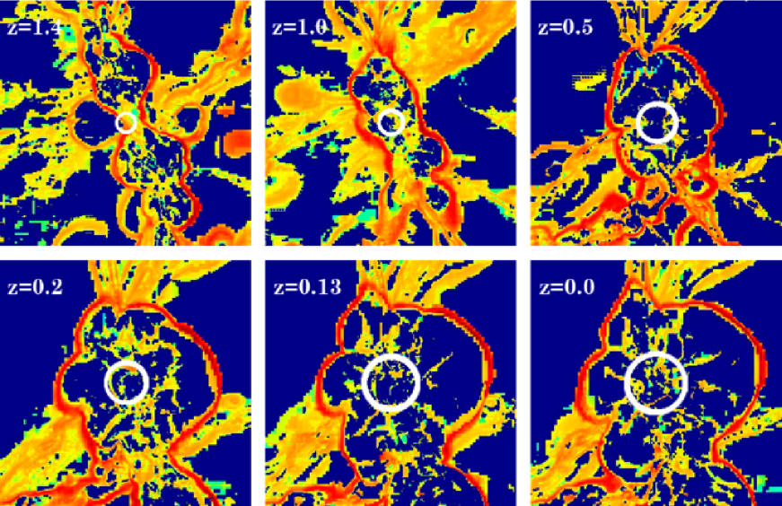
Figure 8: Distribution of shock Mach numbers in logarithmic scale at several redshifts. Each panel is a slice of $0.2$ Mpc thickness and $\sim$ 21 Mpc side length. The white circle in each panel represents the position of the main progenitor of the most massive halo at $z=0$. The redder the color used to plot the shock wave the higher the Mach number.

Besides the qualitative procedure just described, we have tried to track the movement of the accretion shock around the haloes in greater detail. In order to do so, we have visually identified and measured the most relevant quantities of the shocks. Unfortunately, the statistical limitation of our sample of massive haloes, plus the difficulty of the semi-manual methodology to follow the evolution of the accretion shocks, has made extremely difficult to perform this analysis and, as a consequence, we have been able to do it only for the most massive halo in the simulation. In Table 1, we summarise the main data corresponding to the studied halo and its associated external shock wave according to Fig. 8. The measured quantities are: the redshift (z), the cluster virial mass ($M_{vir}$), the cluster virial radius ($R_{vir}$), the comoving radius of the shell defined by the shock ($R_{s}$), and the shock speed ($v_{s}$). The radial distance from the halo centre to the shock, $R_{s}$, is estimated using a visual mechanism which can only produced approximated results. To do so, we make thin slices of the Mach number distribution like the ones plotted in Fig. 8. In these slices, we identify the halo and associate by eye the thin quasi-spherical shell having high and homogenous Mach numbers to the shock wave that wraps the halo. Then, considering several directions, we measure different values for the radial distance from the centre of the halo to the shock front. The final value for the shock radial distance, $R_{s}$, is obtained as the arithmetic mean. Using the same procedure, the modules of the gas velocity at the different points of the shock shell used to estimate $R_{s}$, are computed and averaged to produce the final shock speed, $v_{s}$.

Table 1: Main data describing the most massive halo and its associated external shock wave. The different columns stand for the redshift, z, the halo virial mass, $M_{vir}$, in units of $10^{14}\,M_{\odot}$, the halo virial radius, $R_{vir}$, in comoving Mpc, the radius of the shock wave, $R_{s}$, in comoving Mpc, and the shock speed, $v_{s}$, in $km/s$, respectively.

z	$M_{vir}$	$R_{vir}$	$R_{s}$	$v_{s}$
	$(10^{14}\,M_{\odot})$	$(Mpc)$	$(Mpc)$	(km/s)
0.0	8.3	2.4	9.5	901
0.13	6.1	2.1	8.4	900
0.2	2.9	1.6	7.7	920
0.3	2.7	1.5	6.9	900
0.4	2.6	1.5	6.4	970
0.5	2.8	1.5	5.5	950
0.6	2.2	1.4	4.4	945
0.8	0.92	1.0	3.3	942
1.0	0.81	0.9	2.6	950
1.2	0.61	0.8	2.2	900
1.4	0.46	0.7	1.5	890

The propagation of the shock wave surrounding the considered halo can be well summarised in Fig. 9, where the distance from the shock wave to the halo centre ($R_{s}$) is plotted against the time. As expected, the behaviour is consistent with the self-similar nature of an spherical isolated shock wave, being the slope of the line plotted in Fig. 9 the propagation speed of the shock.

The last column in Table 1 shows the shock speed ($v_{s}$) at different times. These values are consistent with a constant propagation speed. Nevertheless, there are deviations from a perfectly constant slope which are explained by the errors associated to the graphical method used to measure the positions and velocities of the shock wave, and by the non idealised environment surrounding the haloes where the external medium is far from being homogeneous.

Assuming all these uncertainties, we can use Fig. 9 to date the formation time of the studied halo around $z\sim 1.4$ and, therefore, it is nowadays $\sim 8.9\,Gyrs$ old. This redshift is the highest one at which the shock appears perfectly visible and well defined. At early stages, the situation is too messy and the crude method used to track the shock produces too much error. In this sense, this time should be taken as a rough estimate of the collapse of the halo. In any case, it is interesting to compare this formation time of the halo with its half mass formation time which for this particular cluster is $z\sim 0.2$.

Figure 9: Temporal evolution of the shock wave distance to the halo centre.

Under the hypothesis that the shocks associated with haloes could be observed and measured, we suggest the idea to use them as probes to infer the main characteristics of the haloes where they were created. Although the detection and measurement of large-scale shock waves is an observational challenge, there is hope that new coming instruments – i.e., SKA (Square Kilometre Array; e.g., Rawlings et al., 2004; Battaglia et al., 2009) – could shed some light on this scenario.

As it has been already mentioned, the properties of the shock waves have been derived by a graphical method. Besides, our sample is very reduced. Therefore, due to the uncertainties of the method and the statistical limitations, the results of this Section should be interpreted with caution, and only as a way to illustrate the potentiality of the study and observation of the shock waves associated to cosmic structures.

4 Summary and conclusions

In this paper, we focus on the properties of the shock waves developed during the hierarchical evolution of the cosmic structures by means of a cosmological AMR simulation.

To analyse the shock waves, we develop a numerical algorithm able of identifying shocks in 3-D AMR simulations. After labeling all the shocked cells (compression regions with $\nabla\cdot{\bf v}<0$) within the computational box, the Mach numbers of the shocks are computed by means of the Rankine-Hugoniot temperature-jump condition. The Eulerian nature of the adopted numerical scheme allows to accurately detect shocks. Besides, the AMR structure of the employed numerical method produces sets of grids mapping different levels of resolution that naturally permits to find shocks corresponding to different spatial scales.

We analyse the morphology of the shock patterns detected in the simulated volume which turns out to be rather complex. In qualitative agreement with previous works (e.g., Ryu et al., 2003; Pfrommer et al., 2006; Vazza, Brunetti & Gheller, 2009), the shocks morphologies follow the shape of the cosmic web, being filaments, sheets, and haloes surrounded by strong external shocks, while more irregular and weaker internal shocks are found within the virial radius of haloes. From the morphological point of view, it is remarkable that the external shocks associated to the most massive haloes – galaxy clusters – show a quasi-spherical shape around them.

The statistical analysis of the shocks found in the simulation has produced several important conclusions. We have estimated that the filling factor of shocks – the fraction of the total volume occupied by shocked cells – at $z=0$ is roughly the $20\%$ of the simulated volume with a mean Mach number of $\simeq 4$.

Following with this analysis, we have computed the differential shock distribution function within the simulated volume as a function of the shock Mach numbers. This function can be fitted by two different power laws with the form $dN(\mathcal{M})/d\mathcal{M}\propto\mathcal{M}^{\alpha}$, having the low Mach numbers (up to $\simeq 20$) a slope of $\alpha\simeq-1.7$, whereas a steeper relation ($\alpha\simeq-4.1$) stands for stronger shocks. This turn has a crucial meaning as it shows the transition between the scales associated to internal and external shocks. The distribution function also reveals that most part of cosmological shocks are essentially weak shocks ($\mathcal{M}\leq 2$), as already demonstrated by other authors (e.g., Ryu et al., 2003; Pfrommer et al., 2006; Vazza, Brunetti & Gheller, 2009).

In agreement with the information derived from the shock distribution function, we find that the average Mach number within the virial radius of haloes at $z=0$ is $\mathcal{M}\approx 5$. If we look at higher redshifts, this average Mach number is always below $\approx 20-25$, which perfectly correlates with the turn obtained in the shock distribution function.

When haloes, according to their properties, are located in the plane formed by the two axes, virial mass and average Mach number inside the virial radius, we observe two well-separated trends at $z=0$. One stands for a group of haloes with almost constant low Mach numbers (up to 5) which seems to be non dependent on the halo mass. This population of haloes, characterised by low virial Mach numbers, could stem from the primordial formation of structures which have been initially set up in a quasi-relaxed and smooth process.

The second group of haloes spreads all over the range of Mach numbers but showing a clear correlation with the halo masses. They represent the haloes where strong shocks took place during their early evolution as a consequence of early mergers and violent accretion processes. We conclude that the evolution of haloes along the plane $\mathcal{M}-M_{vir}$ is intimately related with their merging history and with their initial set up. In that sense, possible estimates of $\mathcal{M}$ for a given halo could lead to know whether it has suffered merger events in the past, and it may correlate with other relevant features like the existence or not of cool cores.

Finally, we speculate about the possibility that new radio observations may observe the shocks associated with the formation and evolution of the cosmic structures. Assuming that this could be feasible in the near future, we propose to turn the argument around, and to use the main features of shocks – position and strength – to infer import features of the halo harbouring the shock like, for instance, the formation time of the halo, or its total mass. This last application could be a powerful new tool for cluster mass estimation if we are able to detect the accretion shocks with radio observations (e.g., Giacintucci et al., 2008).

Our main conclusion is that shock waves play a crucial role in the formation and evolution of galaxies and galaxy clusters. Despite this general and obvious statement, direct evidence of shocks, both from the cosmic web formation processes (large scales) and those due to cluster merging events (small scales), has been found only in a relatively small number of clusters thanks to observations of radio relics and temperature maps in X-rays. Therefore, we believe that it is necessary to pursue the study of the role of shocks in cosmological context as they are fundamental players in the paradigm of structure formation in the Universe. Their complete theoretical description together with their detection and observation are still a challenge.

References

- Agertz et al. (2007) Agertz O. et al., 2007, MNRAS, 380, 963
- Bagchi et al. (2006) Bagchi, J., Durret, F., Neto, G. B. L., & Paul, S., 2006, Science, 314, 791
- Battaglia et al. (2009) Battaglia, N., Pfrommer, C., Sievers, J. L., Bond, J. R., & Enßlin, T. A., 2009, MNRAS, 155
- Bonafede et al. (2009) Bonafede, A., Giovannini, G., Feretti, L., Govoni, F., & Murgia, M., 2009, A&A, 494, 429
- (5) Bryan G.L., Norman M.L., 1998, ApJ, 495, 80
- Eisenstein & Hu (1998) Eisenstein D.J., Hu W., 1998, ApJ, 511, 5
- Ensslin et al. (1998) Ensslin T. A., Biermann P. L., Klein U., Kohle S., 1998, A&A, 332, 395
- Fabjan et al. (2010) Fabjan, D., Borgani, S., Tornatore, L., et al. 2010, MNRAS, 401, 1670
- Fujita & Sarazin (2001) Fujita Y., Sarazin C.L., 2001, ApJ, 563, 660
- Gabici & Blasi (2003) Gabici S., Blasi P., 2003, ApJ, 583, 695
- Giacintucci et al. (2008) Giacintucci S., Venturi T., Macario G., Dallacasa D., Brunetti G., Markevitch M., Cassano R., Bardelli S., Athreya R., 2008, A&A, 486, 347
- Haart & Madau (1996) Haart F., Madau P., 1996, ApJ, 461, 20
- Hoeft et al. (2008) Hoeft M., Brüggen M., Yepes G., Gottlöber S., & Schwope A., 2008, MNRAS, 391, 1511
- Kang et al. (2007) Kang H., Ryu D., Cen R., Ostriker J.P., 2007, ApJ, 669, 729
- Katz, Weinberg & Hernquist (1996) Katz N., Weinberg D., Hernquist L., 1996, ApJS, 105, 19
- Kennicutt (1998) Kennicutt, R.C., 1998, ApJ, 498, 541
- Lacey & Cole (1993) Lacey C., Cole S., 1993, MNRAS, 262, 627
- Landau & Lifshitz (1966) Landau L. D., Lifshitz E. M., 1966, hydr.book
- LeVeque (1992) LeVeque R.J., 1992, Numerical methods for conservation laws, Birkhäuser Verlag
- Markevitch, Sarazin & Vikhlinin (1999) Markevitch M., Sarazin C. L., Vikhlinin A., 1999, ApJ, 521, 526
- Markevitch et al. (2002) Markevitch M., Gonzalez A. H., David L., Vikhlinin A., Murray S., Forman W., Jones C., Tucker W., 2002, ApJ, 567, L27
- Markevitch & Vikhlinin (2007) Markevitch M., Vikhlinin A., 2007, Physics Reports, 443, 1
- Miniati et al. (2000) Miniati F., Ryu D., Kang H., Jones T. W., Cen R., Ostriker J. P., 2000, ApJ, 542, 608
- Miniati et al. (2001) Miniati F., Ryu D., Kang H., Jones T. W., 2001, ApJ, 559, 59
- Miniati et al. (2001b) Miniati F., Jones T. W., Kang H., Ryu D., 2001, ApJ, 562, 233
- Miniati (2002) Miniati F., 2002, MNRAS, 337, 199
- Pavlidou & Fields (2006) Pavlidou V., Fields B. D., 2006, ApJ, 642, 734
- Pfrommer et al. (2006) Pfrommer C., Springel V., Enßlin T. A., Jubelgas M., 2006, MNRAS, 367,113
- Pfrommer, Enßlin & Springel (2008) Pfrommer C., Enßlin T. A., Springel V., 2008, MNRAS, 385,1211
- Planelles & Quilis (2010) Planelles S., Quilis V., 2010, A&A, 519:A94
- Press & Schechter (1974) Press W. H., Schechter P., 1974, ApJ, 425, 187
- Quilis, Ibáez & Sáez (1998) Quilis V., Ibáez J. M., Sáez D., 1998, ApJ, 502, 518
- Quilis (2004) Quilis V., 2004, MNRAS, 352, 1426
- Rawlings et al. (2004) Rawlings S., Abdalla F.B., Bridle S.L., Blake C.A., Baugh C.M., Greenhill J.L., van der Hulst J.M., 2004, New Astronomy Reviews, 48, 1013
- Ryu et al. (2003) Ryu D., Kang H., Hallman E., Jones T. W., 2003, ApJ, 593, 599
- Sheth & Tormen (1999) Sheth R., Tormen G., 1999, MNRAS, 308, 119
- Skillman et al. (2008) Skillman S. W. , O’Shea B. W., Hallman E. J., Burns J. O., Norman M. L., 2008, ApJ, 689, 1063
- Skillman et al. (2010) Skillman S. W., Hallman E. J., O’Shea B. W., Burns J. O., Smith B. D., Turk M. J., 2010, ApJ, 735, 96
- Springel & Hernquist (2003) Springel V., Hernquist L., 2003, MNRAS, 339, 289
- Sutherland & Dopita (1993) Sutherland R., Dopita M. S., 1993, ApJS, 88, 253
- Theuns et al. (1998) Theuns T., Leonard A., Efstathiou G., Pearce F. R., Thomas P. A, 1998, MNRAS, 301, 478
- van Weeren et al. (2009) van Weeren, R. J., et al., 2009, A&A, 506, 1083
- Vazza, Brunetti & Gheller (2009) Vazza F., Brunetti G., Gheller C., 2009, MNRAS, 395, 1333
- Vazza et al. (2009) Vazza F., Brunetti G., Kritsuk A., Wagner R., Gheller C., Norman M., 2009, A&A, 504, 33
- Vazza et al. (2010) Vazza F., Brunetti G., Gheller C., Brunino R., 2010, New Astronomy, 15, 695
- Vazza et al. (2011) Vazza F., Dolag K., Ryu D., Brunetti G., Gheller C., Kang H., Pfrommer C., 2011, MNRAS, 418, 960
- Venturi et al. (2007) Venturi T., Giacintucci S., Brunetti G., Cassano R., Bardelli S., Dallacasa D., & Setti G., 2007, A&A, 463, 937
- Yepes et al. (1997) Yepes G., Kates R., Khokhlov A., Klypin A., 1997, MNRAS, 284, 235