Non-equilibrium transport with self-consistent renormalised contacts for a single-molecule nanodevice with electron-vibron interaction

Abstract

We present an application of a new formalism to treat the quantum transport properties of fully interacting nanoscale junctions [Phys. Rev. B 84, 235428 (2011)]. We consider a model single-molecule nanojunction in the presence of two kinds of electron-vibron interactions. In terms of electron density matrix, one interaction is diagonal in the central region and the second is off-diagonal in between the central region and the left electrode. We use a non-equilibrium Green’s function technique to calculate the system’s properties in a self-consistent manner. The interaction self-energies are calculated at the Hartree-Fock level in the central region and at the Hartree level for the crossing interaction. Our calculations are performed for different transport regimes ranging from the far off-resonance to the quasi-resonant regime, and for a wide range of parameters. They show that a non-equilibrium (i.e. bias dependent) static (i.e. energy independent) renormalisation is obtained for the nominal hopping matrix element between the left electrode and the central region. Such a renormalisation is highly non-linear and non-monotonic with the applied bias, however it always lead to a reduction of the current, and also affects the resonances in the conductance. Furthermore, we show that the relationship between the non-equilibrium charge susceptibility and dynamical conductance still holds even in the presence of crossing interaction.

I Intro

The theory of quantum transport in nano-scale devices has evolved rapidly over the past decade, as advances in experimental techniques have made it possible to probe transport properties (at different temperatures) down to the single-molecule scale. Furthermore simultaneous measurement of charge and heat transport through single molecules is now also possible Widawsky et al. (2012). The development of accurate theoretical methods for the description of quantum transport at the single-molecule level is essential for continued progress in a number of areas including molecular electronics, spintronics, and thermoelectrics.

One of the longstanding problems of quantum charge transport is the establishment of a theoretical framework which allows for quantitatively accurate predictions of conductance from first principles. The need for methods going beyond the standard approach based on density functional theory combined with Landauer-like elastic scattering Hirose and Tsukada (1994); DiVentra et al. (2000); Taylor et al. (2001); Nardelli et al. (2001); Brandbyge et al. (2002); Gutierrez et al. (2002); Frauenheim et al. (2002); Xue and Ratner (2003); Louis et al. (2003); Thygesen et al. (2003); García-Suárez et al. (2005) has been clear for a number of years. It is only recently that more advanced methods to treat electronic interaction have appeared, for example those based on the many-body $GW$ approximation Strange et al. (2011); Rangel et al. (2011); Darancet et al. (2007). Alternative frameworks to deal with the steady-state or time-dependent transport are given by many-body perturbation theory based on the non-equilibrium (NE) Green’s function (GF) formalism: in these approaches, the interactions and (initial) correlations are taken into account by using conserving approximations for the many-body self-energy Baym (1962); von Barth et al. (2005); van Leeuwen et al. (2006); Kita (2010); Tran (2008); Myöhänen et al. (2008, 2010); Perfetto et al. (2010); Velický et al. (2010); von Friesen et al. (2009).

Other kinds of interactions, e.g. electron-vibron coupling, also play an important role in single-molecule quantum transport. Inelastic tunneling spectroscopy constitutes an important basis for spectroscopy of molecular junctions, yielding insight into the vibrational modes and ultimately the atomic structure of the junction Arroyo et al. (2010). There have been many theoretical investigations focusing on the effect of electron-vibron coupling in molecular and atomic scale wires Ness and Fisher (1999); Ness et al. (2001); Ness and Fisher (2002); Flensberg (2003); Mii et al. (2003); Montgomery et al. (2003); Troisi et al. (2003); Chen et al. (2005a); Lorente and Persson (2000); Frederiksen et al. (2004); Galperin et al. (2004a, b); Mitra et al. (2004); Pecchia et al. (2004); Pecchia and di Carlo (2004); Chen et al. (2005b); Paulsson et al. (2005); Ryndyk and Keller (2005); Sergueev et al. (2005); Viljas et al. (2005); Yamamoto et al. (2005); Cresti et al. (2006); Kula et al. (2006); Paulsson et al. (2006); Ryndyk et al. (2006); Troisi and Ratner (2006); de la Vega et al. (2006); Toroker and Peskin (2007); Frederiksen et al. (2007); Galperin et al. (2007); Ryndyk and Cuniberti (2007); Schmidt et al. (2007); Troisi et al. (2007); Asai (2008); Benesch et al. (2008); Paulsson et al. (2008); Egger and Gogolin (2008); Monturet and Lorente (2008); McEniry et al. (2008); Ryndyk et al. (2009); Schmidt et al. (2008); Tsukada and Mitsutake (2009); Loos et al. (2009); Secker et al. (2011); Härtle and Thoss (2011); Härtle et al. (2011). In all these studies, the interactions have always been considered to be present in the central region (i.e. the molecule) only, and the latter is connected to two non-interacting terminals. Interactions are also assumed not to cross at the contracts between the central region and the leads. When electronic interactions are present throughout the system, as within density-functional theory calculations, they are treated at the mean-field level and do not allow for any inelastic scattering events. However, there are good reasons to believe that such approximations are only valid in a very limited number of practical cases. The interactions, in principle, exist throughout the entire system.

In a recent paper we derived a general expression for the current in nano-scale junctions with interaction present everywhere in the system Ness and Dash (2011). With such a formalism, we can calculate the transport properties in those systems where the interaction is present everywhere. The importance of extended interaction in nano-scale devices has also been addressed, for electron-electron interaction, in recently developed approaches such as Refs. [Strange et al., 2011; Perfetto et al., 2012].

In the present paper, we also consider interactions existing beyond the central region. We apply our recently developed formalism Ness and Dash (2011) for fully interacting systems to a specific model of a single-molecule nanojunction. We focuss on a model system in the presence of electron-vibron interaction within the molecule and between the molecule and one of the leads. We show how the interaction crossing at one interface of the molecular nanojunctions affects the transport properties by renormalising the coupling at the interface in a bias-dependent manner. We also study the relationship between the non-equilibrium charge susceptibility Ness and Dash (2012b) and the dynamical conductance for the present model of interaction crossing at the contacts.

The paper is organised as follows: In Sec. II, we briefly recall the main result of our current expression for fully interacting systems. In Sec. III, we present the model Hamiltonian for the system which include two kinds of electron-vibron interaction, an Holstein-like Hamiltonian combined with a Su-Schrieffer-Heeger-like Hamiltonian. In this section, we also describe how the corresponding self-energies are calculated and the implications of such approximations on the current expression at the left and right interfaces. In Sec. IV, we show that our approximations are fully consistent with the constraint of current conservation. Then the effects of the static non-equilibrium (i.e. energy-independent but bias-dependent) renormalisation of the coupling at the contact on both the current and the dynamical conductance are studied for a wide range of parameters. We also show that the NE charge susceptibility is still related to the dynamical conductance even in the presence of crossing interaction at the contact. We finally conclude and discuss extensions of the present work in Sec. V.

II General theory for quantum transport

We consider a two-terminal device, made of three regions left-central-right, in the steady-state regime. In such a device, labelled $L-C-R$, the interaction—which we specifically leave undefined (e.g. electron-electron or electron-phonon)—is assumed to be well described in terms of the single-particle self-energy $\Sigma^{\rm MB}$ and spreads over the entire system.

We use a compact notation for the Green’s function $G$ and the self-energy $\Sigma$ matrix elements $M(\omega)$. They are annotated $M_{C}$ ($M_{L}$ or $M_{R}$) for the elements in the central region $C$ (left $L$, right $R$ region respectively), and $M_{LC}$ (or $M_{CL}$) and $M_{RC}$ (or $M_{CR}$) for the elements between region $C$ and region $L$ or $R$. There are no direct interactions between the two electrodes, i.e. $\Sigma^{\rm MB}_{LR/RL}=0$.

In Refs. [Ness and Dash, 2011, 2012a], we showed that for a finite applied bias $V$ the steady-state current $I_{L}(V)$ flowing through the left $LC$ interface is given by:

$$\begin{split}I_{L}&=\frac{e}{\hbar}\int\frac{d\omega}{2\pi}\\ &{\rm Tr}_{\{C\}}\left[G^{r}_{C}\tilde{\Upsilon}^{L,l}_{C}+G^{a}_{C}(\tilde{\Upsilon}^{L,l}_{C})^{\dagger}+G^{<}_{C}(\tilde{\Upsilon}^{L}_{C}-(\tilde{\Upsilon}^{L}_{C})^{\dagger})\right]\\ +&{\rm Tr}_{\{L\}}\left[\Sigma^{{\rm MB},>}_{L}G^{<}_{L}-\Sigma^{{\rm MB},<}_{L}G^{>}_{L}\right]\end{split}$$ (1)

where the $\Upsilon_{C}$ quantities are

$$\begin{split}\tilde{\Upsilon}^{L}_{C}(\omega)&=\Sigma^{a}_{CL}(\omega)\ \tilde{g}^{a}_{L}(\omega)\ \Sigma^{r}_{LC}(\omega),\\ (\tilde{\Upsilon}^{L}_{C})^{\dagger}&=\Sigma^{a}_{CL}\ \tilde{g}^{r}_{L}\ \Sigma^{r}_{LC},\\ \tilde{\Upsilon}^{L,l}_{C}&=\Sigma^{<}_{CL}\left(\tilde{g}^{a}_{L}-\tilde{g}^{r}_{L}\right)\Sigma^{r}_{LC}+\Sigma^{r}_{CL}\ \tilde{g}^{<}_{L}\ \Sigma^{r}_{LC}.\end{split}$$ (2)

By definition $\Sigma_{LC}(\omega)=V_{LC}+\Sigma^{\rm MB}_{LC}(\omega)$ (similarly for the $CL$ components) where $V_{LC/CL}$ are the nominal coupling matrix elements between the $L$ and $C$ regions. $\tilde{g}^{x}_{L}(\omega)$ are the GF of the region $L$ renormalised by the interaction inside that region, where $x=r,a,<$ stands for the retarded, advanced and lesser GF components. For example, for the advanded and retarded components, we have $(\tilde{g}^{r/a}_{L}(\omega))^{-1}=({g}^{r/a}_{L}(\omega))^{-1}-\Sigma^{{\rm MB},r/a}_{L}(\omega)$ where all quantities are defined only in the subspace $L$.

The first line in the current equation Eq. (1) corresponds to a generalisation of the Meir and Wingreen Meir and Wingreen (1992) result to the cases for which the interactions are present in the three $L,C,R$ regions as well as in between the $L/C$ and $C/R$ regions. The second trace in Eq. (1) corresponds to inelastic events induced by the interaction in the $L$ lead. When a local detailed balance equation helds, this terms vanishes since locally one has $\Sigma^{{\rm MB},>}G^{<}=\Sigma^{{\rm MB},<}G^{>}$.

Eq. (1) bears some resemblance to the expression derived by Meir and Wingreen Meir and Wingreen (1992) when written as:

$$\begin{split}I_{L}^{\rm MW}&=\frac{e}{\hbar}\int\frac{{\rm d}\omega}{2\pi}\\ &{\rm Tr}_{\{C\}}\left[G^{r}_{C}\Sigma^{L,<}_{C}+G^{a}_{C}(\Sigma^{L,<}_{C})^{\dagger}+G^{<}_{C}(\Sigma^{L,a}_{C}-\Sigma^{L,r}_{C})\right].\end{split}$$ (3)

where we use the definitions $\Sigma^{L,<}_{C}=-(\Sigma^{L,<}_{C})^{\dagger}=V_{CL}\ {g}^{<}_{L}\ V_{LC}={\rm i}f_{L}\Gamma_{L}$ and $\Sigma^{L,a}_{C}-\Sigma^{L,r}_{C}=V_{CL}({g}^{a}_{L}-g^{r}_{L})V_{LC}={\rm i}\Gamma_{L}$. Hence $I_{L}^{\rm MW}$ becomes

Hence one can see by comparing Eq. (1) and Eq. (3) that the quantities $\tilde{\Upsilon}_{LC}$ ($\tilde{\Upsilon}^{\dagger}_{LC}$) and $\tilde{\Upsilon}^{l}_{LC}$ are playing the role of the $L$ lead self-energy $\Sigma^{a}_{L}$ ($\Sigma^{r}_{L}$) and $\Sigma^{<}_{L}$ respectively when the interactions cross at the $LC$ interface. In Meir and Wingreen model, the leads are non-interacting, hence the second trace ${\rm Tr}_{\{L\}}\left[...\right]$ in Eq. (1) does not exist.

III Model for the interaction

III.1 Hamiltonians

We consider a single-molecule junction in the presence of electron-vibron interaction inside the central region and crossing at the contacts. Using a model system to reduce these calculations to a tractable size, we concentrate on a single molecular level coupled to a single vibrational mode. A full description of our methodology, for the interaction inside the region $C$, is provided in Refs. [Dash et al., 2010; Ness et al., 2010; Dash et al., 2011]. Furthermore, we consider that the electron-vibron interaction exist also at one contact (the left $L$ electrode for instance). This model typically corresponds to an experiment for a molecule chemisorbed onto a surface (the left electrode) with a tunneling barrier to the right $R$ lead.

In the following model, we consider two kinds of electron-vibron coupling: a local coupling in the sense of an Holstein-like coupling of the electron charge density with a internal degree of freedom of vibration inside the central region, and an off-diagonal coupling in the sense of a Su-Schrieffer-Heeger-like coupling Heeger et al. (1988); Ness et al. (2001) to another vibration mode involving the hopping of an electron between the central $C$ region and the $L$ electrode.

The Hamiltonian for the region $C$ is

$$\begin{split}H_{C}=\varepsilon_{0}d^{\dagger}d+\hbar\omega_{0}a^{\dagger}a+\gamma_{0}(a^{\dagger}+a)d^{\dagger}d,\end{split}$$ (4)

where $d^{\dagger}$ ($d$) creates (annihilates) an electron in the molecular level $\varepsilon_{0}$. The electron charge density in the molecular level is coupled to the vibration mode of energy $\omega_{0}$ via the coupling constant $\gamma_{0}$, and $a^{\dagger}$ ($a$) creates (annihilates) a vibration quantum in the vibron mode $\omega_{0}$. The central region $C$ is nominally connected to two (left and right) one-dimensional tight-binding chains via the hopping integral $t_{0L}$ and $t_{0R}$. The corresponding electrode $\alpha=L,R$ self-energy is $\Sigma^{r}_{\alpha}(\omega)=t_{0\alpha}^{2}/\beta_{\alpha}\exp^{{\rm i}k_{\alpha}(\omega)}$ with the dispersion relation $\omega=\varepsilon_{\alpha}+2\beta_{\alpha}\cos(k_{\alpha}(\omega))$ where $\varepsilon_{\alpha}$ and $\beta_{\alpha}$ are the tight-binding on-site and off-diagonal elements of the electrode chains.

To describe the electron-vibron interaction existing at the left contact, we consider that the hopping integral $t_{0L}$ is actually dependent on some generalised coordinate $X$. The latter represents either the displacement of the centre-of-mass of the molecule or of some chemical group at the end of the molecule link to the $L$ electrode. At the lowest order, the matrix element can be linearised as $t_{0L}(X)=t_{0L}+t^{\prime}_{0L}X$. Hence the hopping of an electron from the $C$ region to the $L$ region (and vice versa) is coupled to a vibration mode (of energy $\omega_{A}$) via the coupling constant $\gamma_{A}$ (itself related to $t^{\prime}_{0L}$). The corresponding Hamiltonian is given by

$$H_{LC}=\gamma_{A}(b^{\dagger}+b)(c^{\dagger}_{L}d+d^{\dagger}c_{L})+\omega_{A}b^{\dagger}b,$$ (5)

where $b^{\dagger}$ ($b$) creates (annihilates) a vibration quantum in the vibron mode $\omega_{A}$, the generalised coordinate is $X=\sqrt{{\hbar}/{(2m_{A}\omega_{A})}}(b^{\dagger}+b)$, and $c^{\dagger}_{L}$ ($c_{L}$) creates (annihilates) an electron in the level $\varepsilon_{L}$ of the $L$ electrode.

The Hamiltonians Eq. (4) and Eq. (5) are used to calculate the corresponding electron self-energies at different orders of the interaction $\gamma_{0}$ and $\gamma_{A}$ using conventional non-equilibrium diagrammatics techniques Dash et al. (2010, 2011).

Furthermore, at equilibrium, the whole system has a single and well-defined Fermi level $\mu^{\rm eq}$. A finite bias $V$, applied across the junction, lifts the Fermi levels as $\mu_{L,R}=\mu^{\rm eq}+\eta_{L,R}eV$. The fraction of potential drop Datta et al. (1997) at the left contact is $\eta_{L}$ and $\eta_{R}=\eta_{L}-1$ at the right contact, with $\mu_{L}-\mu_{R}=eV$ and $\eta_{L}\in[0,1]$.

III.2 Self-energies for the interactions

The electron-vibron self-energies in the central region $C$ are calculated within the Born approximation. The details of the calculations are reported elsewhere Dash et al. (2010, 2011) so we briefly recall the different expressions for the self-energies $\Sigma^{{\rm MB},x}_{C}=\Sigma^{H,x}_{C}+\Sigma^{F,x}_{C}$ with

$$\begin{split}\Sigma^{H,r}_{C}=\Sigma^{H,a}_{C}=2\frac{\gamma_{0}^{2}}{\omega_{0}}\int\frac{d\omega^{\prime}}{2\pi}iG^{<}_{C}(\omega^{\prime})=-2\frac{\gamma_{0}^{2}}{\omega_{0}}\langle n_{C}\rangle\ ,\end{split}$$ (6)

with $\langle n_{C}\rangle=-i\int{d\omega}/{2\pi}\ G^{<}_{C}(\omega)$ and

$$\Sigma^{F,\lessgtr}_{C}(\omega)=i\gamma_{0}^{2}\int\frac{du}{2\pi}\ D_{0}^{\lessgtr}(u)\ G^{\lessgtr}_{C}(\omega-u)\ ,$$ (7)

and

$$\begin{split}\Sigma^{F,r}_{C}(\omega)=i\gamma_{0}^{2}\int\frac{du}{2\pi}&D_{0}^{r}(\omega-u)\left(G^{<}_{C}(u)+G^{r}_{C}(u)\right)\\ +&D_{0}^{<}(\omega-u)G^{r}_{C}(u)\ ,\end{split}$$ (8)

with the usual definitions for the bare vibron GF $D_{0}^{x}$:

$$\begin{split}D_{0}^{\lessgtr}(\omega)&=-2\pi i\left[\langle N_{0}\rangle\delta(\omega\mp\omega_{0})+\langle{N_{0}}\rangle+1)\delta(\omega\pm\omega_{0})\right]\\ D_{0}^{r}(\omega)&=\frac{1}{\omega-\omega_{0}+i0^{+}}-\frac{1}{\omega+\omega_{0}+i0^{+}}\ ,\end{split}$$ (9)

where $\langle{N_{0}}\rangle$ is the averaged number of excitations in the vibration mode of frequency $\omega_{0}$ given by the Bose-Einstein distribution at temperature $T_{\rm vib}$. In the following, we work in the limit of low temperature for which $\langle N_{0}\rangle=0$.

As a first application of our transport formalism for crossing interactions, we consider a mean-field approximation for the electron-vibron coupling at the $LC$ interface. This leads to the Hartree-like expressions for the many-body self-energies at the $LC$ interface:

$$\Sigma^{{\rm MB},r/a}_{LC}=-2\frac{\gamma_{A}^{2}}{\omega_{A}}\langle n_{LC}\rangle,$$ (10)

where

$$\langle n_{LC}\rangle=-i\int\frac{{\rm d}\omega}{2\pi}\ G^{<}_{LC}(\omega).$$ (11)

Similarly the self-energy $\Sigma^{{\rm MB},r/a}_{CL}$ is obtained from $\langle n_{CL}\rangle=-i\int{\rm d}\omega/{2\pi}\ G^{<}_{CL}(\omega)$.

One can see that the interaction crossing at the $LC$ interface induces a static (however bias-dependent) renormalisation of the nominal coupling $V_{CL}=V_{LC}=t_{0L}$ between the $L$ and $C$ regions. This non-equilibrium renormalisation will induce, amongst other effects, a bias-dependent modification of the broadening of the spectral features of the $C$ region. Since the renormalisation is static at the Hartree level, we use a “potential” notation to represent the normalised coupling: $\Sigma^{r/a}_{LC}\equiv\tilde{V}_{LC}$ with

$$\tilde{V}_{LC}=V_{LC}-2\frac{\gamma_{A}^{2}}{\omega_{A}}\langle n_{LC}\rangle,$$ (12)

and similarly for $\tilde{V}_{CL}$.

The static renormalisation of the nominal coupling $t_{0L}$ is driven by the ratio ${\gamma_{A}^{2}}/{\omega_{A}}$. In the following numerical applications, we consider small to larger renormalisation effects, for which the ratio ${\gamma_{A}^{2}}/({\omega_{A}t_{0L}})$ is ranging from $\sim 0.1$ to $\sim 5.0$. One should note, however, that in all the calculations we have performed, the density matrix element $\langle n_{LC}\rangle$ is always of the order of $10^{-2}$. Therefore the renormalisation effects are always smaller than the nominal coupling $t_{0L}$ itself.

In order to get the renormalised couplings $\tilde{V}_{LC/CL}$, we need the off-diagonal elements $G^{<}_{LC}$ and $G^{<}_{CL}$. The closed expression for the $G^{<}_{LC}$ GF matrix element is obtained from the corresponding Dyson equation $G^{<}_{LC}=[g\Sigma G]^{<}_{LC}$. After formal manipulation, we find that

$$G^{<}_{LC}(\omega)=g^{<}_{L}\tilde{V}_{LC}G^{a}_{C}+G^{r}_{LC}\left(\tilde{V}_{CL}g^{<}_{L}\tilde{V}_{LC}+\Sigma^{<}_{C}+V_{CR}g^{<}_{R}V_{RC}\right)G^{a}_{C},$$ (13)

with $G^{a}_{C}$ is the renormalised advanced GF of the central region

$$G^{a}_{C}(\omega)=\left[[g^{a}_{C}]^{-1}-\Sigma^{a}_{C}-V_{CR}g^{a}_{R}V_{RC}-\tilde{V}_{CL}g^{a}_{L}\tilde{V}_{LC}\right]^{-1},$$ (14)

and the off-diagonal element $G^{r}_{LC}$ is given by

$$G^{r}_{LC}(\omega)=G^{r}_{L}\tilde{V}_{LC}\left[[\tilde{g}^{r}_{C}]^{-1}-V_{CR}g^{r}_{R}V_{RC}\right]^{-1},$$ (15)

where $\tilde{g}^{r}_{C}$ is the renormalised GF of the disconnected C region $[\tilde{g}^{r}_{C}]^{-1}=[g^{r}_{C}]^{-1}-\Sigma^{r}_{C}$. After further manipulation, we get the following expression for $G^{r}_{LC}$ by using the notation $Y_{C}^{R,r}=V_{CR}g^{r}_{R}V_{RC}$ for the non-interacting $R$ lead self-energy:

$$G^{r}_{LC}(\omega)=\left[[g^{r}_{L}]^{-1}-\tilde{V}_{LC}\left[[\tilde{g}^{r}_{C}]^{-1}-Y_{C}^{R,r}\right]^{-1}\tilde{V}_{CL}\right]^{-1}\tilde{V}_{LC}\left[[\tilde{g}^{r}_{C}]^{-1}-Y_{C}^{R,r}\right]^{-1}.$$ (16)

Similarily we can calculate the off-diagonal element $G^{<}_{CL}$ from the corresponding Dyson equations $G^{<}_{CL}=[g\Sigma G]^{<}_{CL}$. We find

$$G^{<}_{CL}(\omega)=G^{r}_{C}\tilde{V}_{CL}g^{<}_{L}+G^{r}_{C}\left(\tilde{V}_{CL}g^{<}_{L}\tilde{V}_{LC}+\Sigma^{<}_{C}+V_{CR}g^{<}_{R}V_{RC}\right)G^{a}_{CL},$$ (17)

where $G^{r}_{C}(\omega)$ is the retarded version of Eq. (14) and

$$G^{a}_{CL}(\omega)=\left[[\tilde{g}^{a}_{C}]^{-1}-Y_{C}^{R,a}\right]^{-1}\tilde{V}_{CL}G^{a}_{L}.$$ (18)

As expected from the definition of the different GFs, we can see that indeed $(G^{<}_{CL}(\omega))^{*}=-G^{<}_{LC}(\omega)$ and $(G^{a}_{CL}(\omega))^{*}=G^{r}_{LC}(\omega)$.

III.3 Calculations

Calculations are performed in a self-consistent manner. There are different ways to calculate the GF and the self-energies in a self-consistent way: in the present work, we first perform self-consistent calculations for the central region $C$. The new hopping matrix elements between the $C$ and $L$ regions given by Eq. (12) are then updated via the use of Eqs. (17) and (13). The calculations are then re-iterated until full self-consistency for all self-energies and GF in the region $C$ and at the left contact $\Sigma^{{\rm MB},r/a}_{LC/CL}$ is obtained.

For the model of crossing interaction we are considering here, further simplications can be introduced in the calculation of the current. Since there is no other interaction inside the $L$ and $R$ regions, the current expression is given only by the first line of Eq.(1). Furthermore, there are no lesser and greater components for the self-energy $\Sigma^{{\rm MB}}_{LC}$ at the mean-field level. The current expression Eq. (1) reduces to:

$$\begin{split}I_{L}&=\frac{e}{\hbar}\int\frac{d\omega}{2\pi}\\ &{\rm Tr}_{\{C\}}\left[G^{r}_{C}\tilde{\Upsilon}^{L,l}_{C}+G^{a}_{C}(\tilde{\Upsilon}^{L,l}_{C})^{\dagger}+G^{<}_{C}(\tilde{\Upsilon}^{L}_{C}-(\tilde{\Upsilon}^{L}_{C})^{\dagger})\right]\ ,\end{split}$$ (19)

with the following simplified expressions for the $\Upsilon_{C}$ quantities

$$\begin{split}\tilde{\Upsilon}^{L}_{C}&=\tilde{V}_{CL}\ {g}^{a}_{L}\ \tilde{V}_{LC},\\ (\tilde{\Upsilon}^{L}_{C})^{\dagger}&=\tilde{V}_{CL}\ {g}^{r}_{L}\ \tilde{V}_{LC},\\ \tilde{\Upsilon}^{L,l}_{C}&=\tilde{V}_{CL}\ {g}^{<}_{L}\ \tilde{V}_{LC},\\ (\tilde{\Upsilon}^{L,l}_{C})^{\dagger}&=-\tilde{V}_{CL}\ {g}^{<}_{L}\ \tilde{V}_{LC},\\ \end{split}$$ (20)

since $\Sigma^{r/a}_{LC}=\tilde{V}_{LC}$ and $\Sigma^{\lessgtr}_{LC}=0$.

Furthermore, the current at the $CR$ interface has a conventional Meir and Wingreen expression, since there are no crossing interactions:

$$\begin{split}I_{R}^{\rm MW}&=-\frac{e}{\hbar}\int\frac{{\rm d}\omega}{2\pi}\\ &{\rm Tr}_{\{C\}}\left[G^{r}_{C}\Sigma^{R,<}_{C}+G^{a}_{C}(\Sigma^{R,<}_{C})^{\dagger}+G^{<}_{C}(\Sigma^{R,a}_{C}-\Sigma^{R,r}_{C})\right]\ ,\end{split}$$ (21)

where we use the conventional definition for the $R$ lead self-energies: $\Sigma^{R,x}_{C}(\omega)=Y_{C}^{R,r}(\omega)=V_{CR}g^{x}_{R}(\omega)V_{RC}$ with $V_{CR}=V_{RC}=t_{0R}$.

The main differences between the expression for the left and right currents $I_{L}$ and $I_{R}^{\rm MW}$ arise from the non-equilibrium static renormalisation of the coupling between the central region $C$ and the $L$ lead given in Eq. (12).

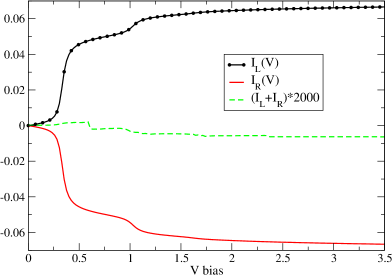
Figure 1: (Color online) Current at the left and right interfaces $I_{L}(V)$ (black line with dots) and $I_{R}(V)$ (red line) given respectively by Eq. (19) and Eq. (21). The current is fully conserved as can be seen by the green dashed line which shows $I_{L}+I_{R}$ magnified by a factor of 2000. The parameters are $\varepsilon_{0}=0.3$, $\omega_{0}=0.30$, $\gamma_{0}=0.21$, $t_{0R}=t_{0L}=0.15$, $\gamma_{A}=0.11$, $\omega_{A}=0.10$, $\beta_{\alpha}=2.0,\epsilon_{\alpha}=0.0$.

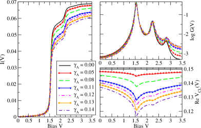
Figure 2: (Color online) Far off-resonant transport regime with $\varepsilon_{0}=0.9$. Current $I(V)$ (left panel), dynamical conductance $G(V)=dI/dV$ in logarithmic scale (top-right panel) and the real part of non-equilibrium renormalized static coupling $V_{CL}(V)$ (bottom-right panel) for different values of the coupling $\gamma_{A}$ strength at the left interface between $0.0$ and $0.14$, corresponding to the follow ratio: ${\gamma_{A}^{2}}/(\omega_{A}t_{0L})=0.0,0.167,0.427,0.807,0.96,1.127,4.667$. The NE renormalization of $\tilde{V}_{CL}(V)$ corresponds to a non-monotonic reduction of the nominal hopping integral $t_{0L}$ with applied bias, which induces a diminution of the current, and modifications of the widths of the conductance peaks accompanied with a slight shift of the conductance peaks at high bias. See text for a complete discussion. The other parameters are $\omega_{0}=0.30$, $\gamma_{0}=0.21$, $t_{0R}=t_{0L}=0.15$, $\gamma_{A}=0.10$, $\beta_{\alpha}=2.0,\epsilon_{\alpha}=0.0$.

IV Results

We have perfomed calculations for many different values of the parameters in the Hamiltonians. We present below the most characteristic results for different transport regimes and for different coupling strengths $\gamma_{A}$, while the interaction in the region $C$ is taken to be in the intermediate coupling regime $\gamma_{0}/\omega_{0}=0.7$. The nominal couplings between the central region and the electrodes $t_{0L,R}$, before NE renormalisation, are not too large, so that we can discrimate clearly between the different vibron side-band peaks in the spectral functions. The values chosen for the parameters are typical values for realistic molecular junctions L. K. Dash and Godby (2012); Dash et al. (2011).

The different transport regimes considered bellow are called the far off-resonant, the off-resonant, the intermediate regime and the quasi-resonant regime. They correspond to different position of the molecular level $\varepsilon_{0}$ with respect to the Fermi level $\mu^{\rm eq}$ at equilibrium. With the static renormalised molecular level $\tilde{\varepsilon}_{0}=\varepsilon_{0}-\gamma_{0}^{2}/\omega_{0}$, the far off-resonant regime corresponding to $\tilde{\varepsilon}_{0}-\mu^{\rm eq}\gg 0$ and $\gg$ several $\omega_{0}$, the off-resonant regime corresponds to $\tilde{\varepsilon}_{0}-\mu^{\rm eq}\gg 0$ and $\sim$ one or two $\omega_{0}$, the intermediate regime corresponds to $\tilde{\varepsilon}_{0}-\mu^{\rm eq}\sim\omega_{0}$ and the quasi-resonant regime corresponds to $\tilde{\varepsilon}_{0}-\mu^{\rm eq}<\omega_{0}$.

In the following the current is given in units of charge per time, the conductance in unit of quantum of conductance $G_{0}=2e^{2}/\hbar$ and the bias $V$ and the normalised coupling $\tilde{V}_{CL}$ in natural units of energy where $e=1$ and $\hbar=1$.

IV.1 Current conservation

One of the most important physical conditions that our formalism needs to fulfil is the constraint of current conservation. We use conserving approximations to calculate the interaction self-energies in the central region $C$ and for the crossing interaction at the left interface. However, since there is no interaction crossing at the $CR$ interface while the interaction is crossing at the $LC$ interface, we have to check that the current given by Eq. (19) for $I_{L}(V)$ is equal to the Meir and Wingreen current given by Eq. (21) for $I_{R}(V)$, i.e. $I_{L}+I_{R}=0$. Figure 1 shows that the condition of current conservation is indeed fulfilled, as expected. We have carefully checked that the current is conserved for all the calculations presented in the present paper, i.e. that $|I_{L}+I_{R}|/|I_{L}|\sim|I_{L}+I_{R}|/|I_{R}|<10^{-5}$.

IV.2 Static non-equilibrium renormalisation

In Figures 2 to 5, we show the dependence of the current $I(V)$, of the dynamical conductance $G(V)=dI/dV$ and of the renormalised coupling $\tilde{V}_{CL}(V)$ on the applied bias $V$, for different values of the interaction strength $\gamma_{A}$ at the left contact. We consider different transport regimes ranging from the far off-resonant regime (Fig. 2), the off-resonant regime (Fig. 3), the intermediate regime (Fig. 4) and finally the quasi-resonant regime (Fig. 5).

The NE renormalisation of the coupling at the left contact given by Eq. (12) corresponds to an effective decrease of the hopping integral leading to a decrease of the current for increasing values of $\gamma_{A}$, as can be seen in the left panels of figs. 2 to 5. The real part of $\tilde{V}_{CL}(V)$ shows a non-monotonic behaviour with the applied bias and presents features (local dips) at applied biases corresponding to peaks in the dynamical conductance (bottom right panels of figs. 2 to 5). Therefore, the interaction crossing at the left contact not only decreases the value of the current but also affects the width of the peaks in the conductance, as can be seen in the top right panels of figs. 2 to 5.

In all our calculations, it appears that each conductance peak now has an asymmetric shape, i.e. a different broadening on each side of the peak, which is due to the non-monotonic and asymmetric behaviour of $\tilde{V}_{CL}$ versus applied bias. The detailed understanding of such a behaviour is rather complex. However, one can obtain a qualitative understanding of our results by considering the following analysis.

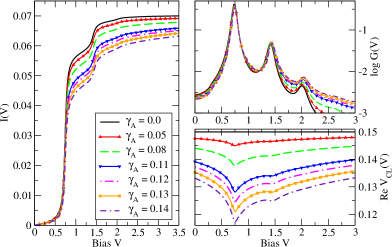
Figure 3: (Color online) Intermediate off-resonant transport regime with $\varepsilon_{0}=0.5$. The other parameters are the same as in figure 2. See text for a complete discussion.

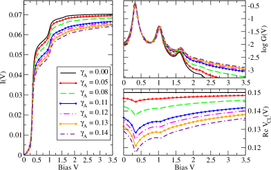
Figure 4: (Color online) Intermediate off-resonant/resonant regime with $\varepsilon_{0}=0.3$. The other parameters are the same as in figure 2. See text for a complete discussion.

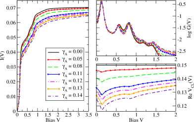
Figure 5: (Color online) Quasi-resonant transport regime with $\varepsilon_{0}=0.2$. Same parameters as in figure 2. See text for a complete discussion.

We can use the current expressions for $I_{L}$ and $I_{R}$ given by Eq. (19) and Eq. (21) respectively to obtain a symmetrized current $I=(I_{L}-I_{R})/2$ expression within a good approximation Meir and Wingreen (1992) :

$$I=\frac{e}{\hbar}\int\frac{d\omega}{2\pi}\ (f_{L}-f_{R})\ \frac{\tilde{\Gamma}_{C}^{L}\Gamma_{C}^{R}}{\tilde{\Gamma}_{C}^{L}+\Gamma_{C}^{R}}\ \pi A_{C}(\omega)\ ,$$ (22)

where $\pi A_{C}(\omega)=-\Im mG_{C}^{r}(\omega)$ and

$$G_{C}^{r}=\left[\omega-\varepsilon_{0}-\Sigma_{C}^{H+F,r}-\tilde{\Sigma}_{C}^{L,r}-\Sigma_{C}^{R,r}\right]^{-1}\ ,$$ (23)

with the self-energy in the central region $\Sigma_{C}^{H+F,r}(\omega)$ given by the sum of Eq. (6) and Eq. (8); and we recall that

$$\begin{split}\tilde{\Sigma}_{C}^{L,r}(\omega)=\tilde{V}_{CL}\ {g}^{r}_{L}(\omega)\ \tilde{V}_{LC}=\Re e\Sigma_{C}^{L,r}-i\tilde{\Gamma}_{C}^{L}/2,\\ \Sigma_{C}^{R,r}(\omega)=V_{CR}\ {g}^{r}_{R}(\omega)\ V_{RC}=\Re e\Sigma_{C}^{R,r}-i\Gamma_{C}^{R}/2.\end{split}$$ (24)

In the off-resonant regime and for small bias $V<\omega_{0}$, one can consider that $\Im m\Sigma_{C}^{H+F,r}\sim 0$ (see Ref. [Ness and Dash, 2011]), hence

$$I\propto\int\frac{d\omega}{2\pi}\ \frac{(f_{L}-f_{R})\ \tilde{\Gamma}_{C}^{L}\Gamma_{C}^{R}}{(\omega-\varepsilon_{0}-\Re e\Sigma_{C}^{\rm tot})^{2}+(\tilde{\Gamma}_{C}^{L}+\Gamma_{C}^{R})^{2}/4}\ .$$ (25)

We can now use Eq. (25) to understand the behaviour of the current. In Figure 6 we show the parametric curves $I(V)-\tilde{V}_{CL}(V)$ obtained for the far off-resonant transport regime (shown in Fig. 2). Figure 6 shows a complex dependence of the current versus the NE renormalised coupling $\tilde{V}_{CL}$. However at low bias, one can consider that $\tilde{\Gamma}_{C}^{L}$ and $\Gamma_{C}^{R}$ are independent of $\omega$ and hence take such quantities out of the integral in Eq. (25). Therefore we have $I\propto\tilde{\Gamma}_{C}^{L}$ and the current is quadratic in $\tilde{V}_{CL}$ since $\tilde{\Gamma}_{C}^{L}\propto(\tilde{V}_{CL})^{2}$. Such a dependence can be clearly seen in Figure 6 for the low bias regime where $I_{L}<0.01$.

At larger bias, one can no longer neglect the $\omega$ dependence of $\tilde{\Gamma}_{C}^{L}$ (and $\Gamma_{C}^{R}$) and more importantly the effects of the interaction in the central region, i.e. $\Im m\Sigma_{C}^{H+F,r}\neq 0$. Hence the quadratic dependence of $I$ on $V_{CL}$ is lost.

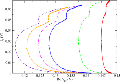
Figure 6: (Color online) Parametric curve $I(V)-\tilde{V}_{CL}(V)$ for the far off-resonant transport regime shown in Fig. 2 (using the same legend for the different $\gamma_{A}$ values). The starting points of the parametric curves, i.e. $V=0$, are at the bottom of the graph (zero current values), and increasing $V$ corresponds to increasing values of the current. At low bias ($I_{L}<0.01$), $I_{L}$ is quadratic in $\tilde{V}_{CL}$.

We now turn onto the effect of the strength of the nominal hopping integral $t_{0L}$ on the renormalised coupling $\tilde{V}_{CL}(V)$ at fixed values of the crossing interaction strength $\gamma_{A}$. Figure 7 shows the relative dependence of $\tilde{V}_{CL}(V)$ on the nominal coupling $t_{0L}$ at the left interface versus applied bias. The figure shows that there is no simple relationship between $\tilde{V}_{CL}(V)$ and $t_{0L}$ for the whole range of parameters explored. There is a small linear regime at low applied bias, otherwise the dependence of $\tilde{V}_{CL}$ on both $t_{0\alpha}$ and $V$ is highly non-linear. There is a progressive washing-out of the features in $\tilde{V}_{CL}(V)$ for increasing values of $t_{0\alpha}$, since a general increase of the coupling to the leads generates to a global broadening of the features in the spectral functions.

IV.3 Non-equilibrium charge susceptibility

In a recent paper Ness and Dash (2012b), we have developed the concept of the generalized susceptibilities for nonlinear systems Safi and Joyez (2011) and applied it to the charge transport properties in two-terminal nano-devices. We have introduced the non-equilibrium charge susceptibility $\chi_{c}^{\rm NE}(V)$ concept, defined by $\chi_{c}^{\rm NE}(V)=\partial\langle n_{C}\rangle/\partial V$. We have shown that $\chi_{c}^{\rm NE}(V)$ is related to the dynamical conductance $G(V)$. The relationship is formally different than the one obtained at equilibrium. In spectroscopic terms, both $\chi_{c}^{\rm NE}(V)$ and $G(V)$ contain features versus applied bias when charge fluctuation occurs in the corresponding electronic resonance. This relationship has been demonstrated for model calculations of interacting nanoscale devices but only when the interaction is present in the central region Ness and Dash (2012b). We now check the validity of such a relationship between $\chi_{c}^{\rm NE}(V)$ and $G(V)$ when interaction crossing at the left contact is also taken into account.

Figure 8 shows the results we obtain for $\chi_{c}^{\rm NE}(V)$ and $G(V)$ for different sets of parameters corresponding to the off-resonant and quasi-resonant transport regimes. Once more, we find that $\chi_{c}^{\rm NE}(V)$ and $G(V)$ present features at the same applied bias. Such a behaviour validates the relationship between the non-equilibrium charge susceptibility and the dynamical conductance even when interactions cross at the contacts (at least at the static mean-field level).

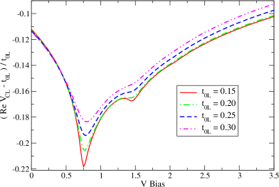
Figure 7: (Color online) Renormalised coupling $\tilde{V}_{CL}(V)$ for the off-resonant transport regime ($\varepsilon_{0}=0.50$) and $\gamma_{A}=0.14$ versus applied bias and for different values of the nominal hopping integrals $t_{0\alpha}$ ($\alpha=L,R$). The relative dependence of $\tilde{V}_{CL}$, shown here for $(\Re e\tilde{V}_{CL}(V)-t_{0\alpha})/t_{0\alpha}$, is linear only for small bias. Otherwise the dependence of $\tilde{V}_{CL}$ on both $t_{0\alpha}$ and $V$ is highly non-linear. The other parameters are the same as in Fig. 3.

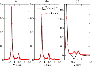
Figure 8: (Color online) Non-equilibrium charge susceptibility $\chi_{c}^{\rm NE}(V)$ and dynamical conductance $G(V)$ versus applied bias for different sets of parameters. $\chi_{c}^{\rm NE}(V)$ is rescaled by a factor of 7. (a) Off-resonant regime $\varepsilon_{0}=0.5$ and $\gamma_{A}=0.08$. (b) Off-resonant regime $\varepsilon_{0}=0.5$ and $\gamma_{A}=0.14$, (c) Quasi-resonant regime $\varepsilon_{0}=0.2$ and $\gamma_{A}=0.05$. $\chi_{c}^{\rm NE}(V)$ and $G(V)$ present features at the same applied bias. Note the negative contribution to $\chi_{c}^{\rm NE}$ around $V\sim 0.56$. See main text for a complete discussion. The other parameters are the same as in Fig. 3.

Finally, one should note the negative contribution to $\chi_{c}^{\rm NE}(V)$ in panel (c) of Figure 8. Such a behaviour originates from the properties of $\chi_{c}^{\rm NE}$ and not from the approximation used to calculate the crossing interaction Ness:unpub2012 . In fact, there are always two contributions to $\chi_{c}^{\rm NE}$, one is positive and corresponds to electron fluctuation and the other is negative and corresponds to hole fluctuation. By electron (hole) fluctuations, we mean the variation of the occupancy (versus applied bias) of electronic resonances located nominally above (below) the Fermi level at equilibrium (or at small bias). Therefore, for the off-resonant transport regime with $\varepsilon_{0}\gg\mu^{\rm eq}$, the features in $\chi_{c}^{\rm NE}(V)$ corresponds to positive peaks (as shown in Panels (a) and (b) in Figure 8 and in the different figures of Ref. [Ness and Dash, 2012b]). For the off-resonant regime with $\varepsilon_{0}\ll\mu^{\rm eq}$, one would get negative peaks in $\chi_{c}^{\rm NE}(V)$. For the intermediate and quasi-resonant transport regime, one obtains both positive and negative contributions in $\chi_{c}^{\rm NE}(V)$ as shown in panel (c) of Figure 8. The most peculiar case corresponds to a fully electron-hole symmetric system, i.e. the spectral function $A_{C}(\omega)$ is fully symmetric around the equilibrium Fermi level and for any applied bias $V$ with $\mu_{L,R}=\mu^{\rm eq}\pm eV/2$. In that case, one can easily show that $\langle n_{C}\rangle=-i\int{\rm d}\omega\ G_{C}^{<}(\omega)/2\pi$ is actually given by $\langle n_{C}\rangle\sim\int_{-\infty}^{+\infty}{\rm d}\omega\ A_{C}(\omega)$ for symmetry reasons. Hence $\langle n_{C}\rangle$ is independent of the applied bias for conserving approximations for the self-energies, and consequently $\chi_{c}^{\rm NE}(V)=0$. Such a behaviour can also be interpreted with the previous picture: for a fully electron-hole symmetric system, any contributions from electron fluctuation is exactly cancelled out by the opposite contribution from hole fluctuation, and $\chi_{c}^{\rm NE}(V)$ is flat and equal to zero for each bias Ness:unpub2012 .

V Conclusion

We have studied the transport properties through a two-terminal nanoscale device with interactions present not only in the central region but also with interaction crossing at the interface between the left lead and the central region. To calculate the current for such an fully interacting system, we have used our recently developed quantum transport formula Ness and Dash (2011) based on the NEGF formalism. As a first practical application, we have considered a prototypical single-molecule nanojunction with electron-vibron interaction. In terms of the electron density matrix, the interaction is diagonal in the central region for the first vibron mode and off-diagonal between the central region and the left electrode for the second vibron mode. The interaction self-energies are calculated in a self-consistent manner using the lowest order Hartree-Fock-like diagram in the central region and the Hartree-like diagram for the crossing interaction. Our calculations were performed for different transport regimes ranging from the far off-resonance to the quasi-resonant regime, and for a wide range of parameter values. They shown that, for this model, we obtain a non-equilibrium (i.e. bias dependent) static (i.e. energy independent) renormalisation of the nominal hopping matrix element between the left electrode and the central region. The renormalisation is such that the amplitude of the current is reduced in comparison with the current values obtained when the interaction is only present in the central region. Such a result could provide an partial explanation for the fact in conventional density-functional based calculations, the values of the current are always much larger than in the corresponding experiments, since no non-equilibrium renormalisation of the contacts is taken into account in those calculations. However, even though it provides the right trends, the decrease in the current obtained by NE renormalisation of the coupling to the leads is not as important as the effects obtained from a proper calculation of the band-gap and band-alignment in realistic molecular system Toher and Sanvito (2007); Thygesen (2008); Rostgaard et al. (2010); Strange et al. (2011).

The NE static renormalisation of the contact is highly non-linear and non-monotonic in function of the applied bias, and the larger effects occur at applied bias corresponding to resonance peaks in the dynamical conductance. The conductance is also affected by the NE renormalisation of the contact, showing asymmetric broadening around the resonance peaks and some slight displacement of the peaks at large bias in function of the coupling strengh $\gamma_{A}$.

Furthermore, we have also shown that, even in the presence of crossing interactions, the relationship between the NE charge susceptibility and dynamical conductance Ness and Dash (2012b) still holds for the different transport regimes considered here.

Extensions of the present study are now considered. One route is to develop more accurate NE renormalisation by considering, for example, a quasi-particle approach within a dynamical mean-field-like treatement of the crossing interaction self-energy Ness:unpub2012 . Another route is to go beyond the Hartree approximation for the crossing interaction self-energy using other many-body diagrams Dash et al. (2011). This would lead to dynamical NE renormalisation of the contact involving inelastic scattering processes.

Finally, it should be noted that for the model system we considered here, one could also solve the problem by using more standard approaches (typically the original Meir and Wingreen approach) by extending the size of the central region to include all the interaction. The results then obtained should be strictly equivalent to our calculations. We have already commented in detail on this point (in a formal and theoretical point of view) in Refs.[Ness and Dash, 2012a, 2011]. However our approach offers a more intuitive physical interpretation of the results, i.e. renormalisation of the contact (in the present case in a static NE mean-field scheme). Using an extended central region will not provide an easy physical interpretation of the results; and as a matter of principle, it will not always be possible to increase at will the size of the central region, more especially when one considers future application of the method to much large molecular system with much more complex coupling to the leads.

References

- Widawsky et al. (2012) J. R. Widawsky, P. Darancet, J. B. Neaton, and L. Venkataraman, Nano Letters 12, 354 (2012).
- Hirose and Tsukada (1994) K. Hirose and M. Tsukada, Physical Review Letters 73, 150 (1994).
- DiVentra et al. (2000) M. DiVentra, S. T. Pantelides, and N. D. Lang, Physical Review Letters 84, 979 (2000).
- Taylor et al. (2001) J. Taylor, H. Guo, and J. Wang, Physical Review B 63, 245407 (2001).
- Nardelli et al. (2001) M. B. Nardelli, J.-L. Fattebert, and J. Bernholc, Physical Review B 64, 245423 (2001).
- Brandbyge et al. (2002) M. Brandbyge, J.-L. Mozos, P. Ordejón, J. Taylor, and K. Stokbro, Physical Review B 65, 165401 (2002).
- Gutierrez et al. (2002) R. Gutierrez, G. Fagas, G. Cuniberti, F. Grossmann, R. Schmidt, and K. Richter, Physical Review B 65, 113410 (2002).
- Frauenheim et al. (2002) T. Frauenheim, G. Seifert, M. Elstner, T. Niehaus, C. Köhler, M. Amkreutz, M. Sternberg, Z. Hajnal, A. D. Carlo, and S. Suhai, Journal of Physics: Condensed Matter 14, 3015 (2002).
- Xue and Ratner (2003) Y. Xue and M. A. Ratner, Physical Review B 68, 115406 (2003).
- Louis et al. (2003) E. Louis, J. A. Vergés, J. J. Palacios, A. J. Pérez-Jiménez, and E. SanFabiàn, Physical Review B 67, 155321 (2003).
- Thygesen et al. (2003) K. S. Thygesen, M. V. Bollinger, and K. W. Jacobsen, Physical Review B 67, 115404 (2003).
- García-Suárez et al. (2005) V. M. García-Suárez, A. R. Rocha, S. W. Bailey, C. J. Lambert, S. Sanvito, and J. Ferrer, Physical Review B 72, 045437 (2005).
- Strange et al. (2011) M. Strange, C. Rostgaard, H. Häkkinen, and K. S. Thygesen, Physical Review B 83, 115108 (2011).
- Rangel et al. (2011) T. Rangel, A. Ferretti, P. E. Trevisanutto, V. Olevano, and G.-M. Rignanese, Phys. Rev. B 84, 045426 (2011).
- Darancet et al. (2007) P. Darancet, A. Ferretti, D. Mayou, and V. Olevano, Phys. Rev. B 75, 075102 (2007).
- Baym (1962) G. Baym, Physical Review 127, 1391 (1962).
- von Barth et al. (2005) U. von Barth, N. E. Dahlen, R. van Leeuwen, and G. Stefanucci, Physical Review B 72, 235109 (2005).
- van Leeuwen et al. (2006) R. van Leeuwen, N. E. Dahlen, G. Stefanucci, C.-O. Almbladh, and U. von Barth, Lecture Notes in Physics 706, 33 (2006).
- Kita (2010) T. Kita, Progress of Theoretical Physics 123, 581 (2010).
- Tran (2008) M.-T. Tran, Physical Review B 78, 125103 (2008).
- Myöhänen et al. (2008) P. Myöhänen, A. Stan, G. Stefanucci, and R. van Leeuwen, EuroPhysics Letters 84, 67001 (2008).
- Myöhänen et al. (2010) P. Myöhänen, A. Stan, G. Stefanucci, and R. van Leeuwen, Journal of Physics: Conference Series 220, 012017 (2010).
- Perfetto et al. (2010) E. Perfetto, G. Stefanucci, and M. Cini, Physical Review Letters 105, 156802 (2010).
- Velický et al. (2010) B. Velický, A. Kalvová, and V. Špička, Physical Review B 81, 235116 (2010).
- von Friesen et al. (2009) M. P. von Friesen, C. Verdozzi, and C.-O. Almbladh, Physical Review Letters 103, 176404 (2009).
- Arroyo et al. (2010) C. R. Arroyo, T. Frederiksen, G. Rubio-Bollinger, M. Vélez, A. Arnau, D. Sánchez-Portal, and N. Agraït, Physical Review B 81, 075405 (2010).
- Ness and Fisher (1999) H. Ness and A. J. Fisher, Physical Review Letters 83, 452 (1999).
- Ness et al. (2001) H. Ness, S. A. Shevlin, and A. J. Fisher, Physical Review B 63, 125422 (2001).
- Ness and Fisher (2002) H. Ness and A. J. Fisher, Europhysics Letters 57, 885 (2002).
- Flensberg (2003) K. Flensberg, Physical Review B 68, 205323 (2003).
- Mii et al. (2003) T. Mii, S. Tikhodeev, and H. Ueba, Physical Review B 68, 205406 (2003).
- Montgomery et al. (2003) M. J. Montgomery, J. Hoekstra, A. P. Sutton, and T. N. Todorov, Journal of Physics: Condensed Matter 15, 731 (2003).
- Troisi et al. (2003) A. Troisi, M. A. Ratner, and A. Nitzan, Journal of Chemical Physics 118, 6072 (2003).
- Chen et al. (2005a) Y. C. Chen, M. Zwolak, and M. di Ventra, Nano Letters 4, 1709 (2005a).
- Lorente and Persson (2000) N. Lorente and M. Persson, Physical Review Letters 85, 2997 (2000).
- Frederiksen et al. (2004) T. Frederiksen, M. Brandbyge, N. Lorente, and A. P. Jauho, Physical Review Letters 93, 256601 (2004).
- Galperin et al. (2004a) M. Galperin, M. A. Ratner, and A. Nitzan, Nano Letters 4, 1605 (2004a).
- Galperin et al. (2004b) M. Galperin, M. A. Ratner, and A. Nitzan, Journal of Chemical Physics 121, 11965 (2004b).
- Mitra et al. (2004) A. Mitra, I. Aleiner, and A. J. Millis, Physical Review B 69, 245302 (2004).
- Pecchia et al. (2004) A. Pecchia, A. di Carlo, A. Gagliardi, S. Sanna, T. Frauenhein, and R. Gutierrez, Nano Letters 4, 2109 (2004).
- Pecchia and di Carlo (2004) A. Pecchia and A. di Carlo, Reports on Progress in Physics 67, 1497 (2004).
- Chen et al. (2005b) Z. Chen, R. Lü, and B. Zhu, Physical Review B 71, 165324 (2005b).
- Paulsson et al. (2005) M. Paulsson, T. Frederiksen, and M. Brandbyge, Physical Review B 72, 201101 (2005).
- Ryndyk and Keller (2005) D. A. Ryndyk and J. Keller, Physical Review B 71, 073305 (2005).
- Sergueev et al. (2005) N. Sergueev, D. Roubtsov, and H. Guo, Physical Review Letters 95, 146803 (2005).
- Viljas et al. (2005) J. K. Viljas, J. C. Cuevas, F. Pauly, and M. Häfner, Physical Review B 72, 245415 (2005).
- Yamamoto et al. (2005) T. Yamamoto, K. Watanabe, and S. Watanabe, Physical Review Letters 95, 065501 (2005).
- Cresti et al. (2006) A. Cresti, G. Grosso, and G. P. Parravicini, Journal of Physics: Condensed Matter 18, 10059 (2006).
- Kula et al. (2006) M. Kula, J. Jiang, and Y. Luo, Nano Letters 6, 1693 (2006).
- Paulsson et al. (2006) M. Paulsson, T. Frederiksen, and M. Brandbyge, Nano Letters 6, 258 (2006).
- Ryndyk et al. (2006) D. A. Ryndyk, M. Hartung, and G. Cuniberti, Physical Review B 73, 045420 (2006).
- Troisi and Ratner (2006) A. Troisi and M. A. Ratner, Nano Letters 6, 1784 (2006).
- de la Vega et al. (2006) L. de la Vega, A. Martín-Rodero, N. Agraït, and A. Levy-Yeyati, Physical Review B 73, 075428 (2006).
- Toroker and Peskin (2007) M. C. Toroker and U. Peskin, Journal of Chemical Physics 127, 154706 (2007).
- Frederiksen et al. (2007) T. Frederiksen, M. Paulsson, M. Brandbyge, and A.-P. Jauho, Physical Review B 75, 205413 (2007).
- Galperin et al. (2007) M. Galperin, A. Nitzan, and M. A. Ratner, Physical Review B 74, 075326 (2007).
- Ryndyk and Cuniberti (2007) D. A. Ryndyk and G. Cuniberti, Physical Review B 76, 155430 (2007).
- Schmidt et al. (2007) B. B. Schmidt, M. H. Hettler, and G. Schön, Physical Review B 75, 115125 (2007).
- Troisi et al. (2007) A. Troisi, J. M. Beebe, L. B. Picraux, R. D. van Zee, D. R. Stewart, M. A. Ratner, and J. G. Kushmerick, Proceedings of the National Academy of Sciences of the USA 104, 14255 (2007).
- Asai (2008) Y. Asai, Physical Review B 78, 045434 (2008).
- Benesch et al. (2008) C. Benesch, M. Čížek, J. Klimeš, I. Kondov, M. Thoss, and W. Domcke, Journal of Physical Chemistry C 112, 9880 (2008).
- Paulsson et al. (2008) M. Paulsson, T. Frederiksen, H. Ueba, N. Lorente, and M. Brandbyge, Physical Review Letters 100, 226604 (2008).
- Egger and Gogolin (2008) R. Egger and A. O. Gogolin, Physical Review B 77, 113405 (2008).
- Monturet and Lorente (2008) S. Monturet and N. Lorente, Physical Review B 78, 035445 (2008).
- McEniry et al. (2008) E. J. McEniry, T. Frederiksen, T. N. Todorov, D. Dundas, and A. P. Horsfield, Physical Review B 78, 035446 (2008).
- Ryndyk et al. (2009) D. A. Ryndyk, R. Gutiérrez, B. Song, and G. Cuniberti, in Energy Transfer Dynamics in Biomaterial Systems, edited by I. Burghardt, V. May, D. A. Micha, and E. R. Bittner (Springer Berlin Heidelberg, 2009), vol. 93 of Springer Series in Chemical Physics, pp. 213–335, ISBN 978-3-642-02306-4.
- Schmidt et al. (2008) B. B. Schmidt, M. H. Hettler, and G. Schön, Physical Review B (Condensed Matter and Materials Physics) 77, 165337 (2008).
- Tsukada and Mitsutake (2009) M. Tsukada and K. Mitsutake, Journal of the Physical Society of Japan 78, 084701 (2009).
- Loos et al. (2009) J. Loos, T. Koch, A. Alvermann, A. R. Bishop, and H. Fehske, Journal of Physics: Condensed Matter 21, 395601 (2009).
- Secker et al. (2011) D. Secker, S. Wagner, S. Ballmann, R. Hartle, M. Thoss, and H. B. Weber, Physical Review Letters 106, 136807 (2011).
- Härtle and Thoss (2011) R. Härtle and M. Thoss, Physical Review B 83, 115414 (2011).
- Härtle et al. (2011) R. Härtle, M. Butzin, O. Rubio-Pons, and M. Thoss, Physical Review Letters 107, 046802 (2011).
- Ness and Dash (2011) H. Ness and L. Dash, Physical Review B 84, 235428 (2011).
- Ness and Dash (2012a) H. Ness and L. Dash, Journal of Physics A: Mathematical and Theoretical 45, 195301 (2012a).
- Meir and Wingreen (1992) Y. Meir and N. S. Wingreen, Physical Review Letters 68, 2512 (1992).
- Perfetto et al. (2012) E. Perfetto, G. Stefanucci, and M. Cini, Physical Review B 85, 165437 (2012).
- Ness and Dash (2012b) H. Ness and L. Dash, Physical Review Letters 108, 126401 (2012b).
- Dash et al. (2010) L. K. Dash, H. Ness, and R. W. Godby, Journal of Chemical Physics 132, 104113 (2010).
- Ness et al. (2010) H. Ness, L. Dash, and R. W. Godby, Physical Review B 82, 085426 (2010).
- Dash et al. (2011) L. K. Dash, H. Ness, and R. W. Godby, Physical Review B 84, 085433 (2011).
- Heeger et al. (1988) A. J. Heeger, S. Kivelson, J. R. Schrieffer, and W.-P. Su, Review of Modern Physics 60, 781 (1988).
- Datta et al. (1997) S. Datta, W. D. Tian, S. H. Hong, R. Reifenberger, J. I. Henderson, and C. P. Kubiak, Physical Review Letters 79, 2530 (1997).
- L. K. Dash and Godby (2012) M. V. L. K. Dash, H. Ness and R. W. Godby, Journal of Chemical Physics 136, 064708 (2012).
- Safi and Joyez (2011) I. Safi and P. Joyez, Physical Review B 84, 205129 (2011).
- (85) H. Ness and L. K. Dash, unpublished.
- Toher and Sanvito (2007) C. Toher and S. Sanvito, Physical Review Letters 99, 056801 (2007).
- Thygesen (2008) K. S. Thygesen, Physical Review Letters 100, 166804 (2008).
- Rostgaard et al. (2010) C. Rostgaard, K. W. Jacobsen, and K. S. Thygesen, Physical Review B 81, 085103 (2010).