Easy-axis ferromagnetic chain on a metallic surface

Abstract

The phases and excitation spectrum of an easy-axis ferromagnetic chain of $S=1/2$ magnetic impurities built on the top of a clean metallic surface are studied. As a function of the (Kondo) coupling to the metallic surface and at low temperatures, the spin chain exhibits a quantum phase transition from an Ising ferromagnetic phase with long-range order to a paramagnetic phase where quantum fluctuations destroy the magnetic order. In the paramagnetic phase, the system consists of a chain of Kondo-singlets where the impurities are completely screened by the metallic host. In the ferromagnetic phase, the excitations above the Ising gap are damped magnons, with a finite lifetime arising due to the coupling to the substrate. We discuss the experimental consequences of our results to spin-polarized electron energy loss spectroscopy (SPEELS), and we finally analyze possible extensions to spin chains with $S>1/2$.

1 Introduction

Recent progress in scanning tunneling microscopy (STM) and other surface-manipulation techniques at the atomic scale has made it possible to build low-dimensional magnetic structures with unprecedented control [1, 2]. Atomic-scale magnetic structures possess an enormous potential for applications in spintronics as well as in classical and quantum computation due to their ability to store and process (quantum) information in the atomic spins. However, in order to build reliable atomic-size memories or qubits out of such systems, it is crucial to understand how the coupling to the environment affects their properties. For instance, it is known that quantum nanomagnets coupled to electronic degrees of freedom are prone to the effects of decoherence induced by Ohmic quantum dissipation [3, 4].

In addition to their interest for information technologies, low-dimensional magnetic systems coupled to dissipative environments are also very important from the point of view of fundamental physics. This is because they allow to study the crossover from quantum to classical behavior as the coupling to the environment is increased [5, 4]. Current theoretical models that describe local quantum degrees of freedom coupled to sources of dissipation predict rich and interesting physical phenomena at low temperatures, including quantum phase transitions and quantum criticality [6, 7, 8, 9], as well as broken continuous symmetries and long-range order (LRO) in low-dimensional systems [10, 11, 12, 13, 14, 15]. The interplay between quantum fluctuations, which are induced by quantum confinement and reduced dimensionality, and quantum dissipation, caused by the interaction with the environment, is at the core of this exotic behavior. From this perspective, magnetic nanostructures built on the top of clean metals offer a unique platform to test our understanding on dissipative quantum systems. For instance, the simplest zero-dimensional (0D) case of a single magnetic impurity coupled to a metallic environment [such like a Co or Mn adatom sitting on a Au(111) surface] is a practical realization of the celebrated Kondo effect, one of the most paradigmatic phenomena in the physics of strongly correlated electrons [16]. This phenomenon is the spin-compensation by the conduction electrons of the magnetic moment $\mathbf{S}_{i}$ of an impurity embedded in a metallic host at temperatures $T\ll T_{K}$, where $T_{K}$ is the so-called Kondo temperature. Eventually, at $T=0$, the ground state of the system is a many-body singlet (termed a ‘Kondo singlet’), formed by a linear superposition of $\mathbf{S}_{i}$ and the spin of a cloud of conduction electrons that is anti-ferromagnetically correlated with the impurity local moment. The original magnetic impurity $\mathbf{S}_{i}$ is thus completely screened by the metallic environment. In the context of magnetic adatoms deposited on clean metallic surfaces, this is a well-established phenomenon, which reveals itself as a narrow Fano resonance at the Fermi energy in the STS spectra [17, 18, 19].

Unfortunately, the extension of the single Kondo impurity to the case of many interacting magnetic impurities embedded in a metallic host represents a formidable theoretical challenge. Due to the many-body nature of the problem, exact methods are only limited to simple cases (i.e., consisting of few magnetic impurities), and at the cost expensive numerical calculations [20]. On the other hand, dynamical mean-field theory (DMFT) methods [21] provide reliable results in the case of bulk 3D compounds, but are much less successful when applied to low-dimensional systems.

One particular class of such low-dimensional systems, namely, one-dimensional (1D) chains of magnetic atoms or organic molecules with active magnetic atoms, are currently under intensive experimental investigation [22, 23, 24, 25, 26]. Thus, by depositing $\simeq 0.1$ monolayer (ML) of Co on Pt(997), which is a vicinal surface containing steps, chains of magnetic atoms have been recently created [22]. The magnetic Co atoms decorate the steps and form ferromagnetic chains, which, when probed by an external magnetic field, typically exhibit superparamagnetism. However, in the case of Co chains at temperatures $T\lesssim 8$ K, the magneto-crystalline anisotropy results in relaxation times which are longer than the experimental typical timescale, and the response of the system becomes effectively ferromagnetic [22]. Another recently reported system, consisting of chains of Co atoms on Cu(775), has been shown to undergo a Peierls distortion leading to dimerization [27]. This dimerized phase has been explained by the strong correlations existing in the partially filled $d$ shells of the Co atoms, which are in the high spin configuration. Maintaining the high spin in a geometry where the overlap between the d orbitals is small and correlations are strong, favors a ferromagnetic ground state, which in turn makes the charge-density wave instability possible.

In the above-mentioned systems, the coupling to the metallic substrate was assumed to be weak, and therefore was neglected in their analysis. However, as we show below, the metallic environment can have dramatic effects for the phase diagram at low temperatures, and it cannot be neglected when studying the magnetic excitations of the chain. With these systems in mind, in this contribution we focus on the analysis of an easy-axis ferromagnetic (FM) 1D spin chain deposited on the top of a metallic surface. Interestingly, as a function of the coupling with the substrate, we predict a quantum phase transition from an Ising ferromagnetic phase with long range order to a paramagnetic phase where quantum fluctuations proliferate and destroy the ordered phase. Although modifying the coupling to the substrate in the experimental systems created so far may be hard, in the future other systems can be created where the coupling to the substrate could be tuned, uncovering even more interesting phenomena.

The article is organized as follows: In the next Section, we introduce a simple model to describe an easy-axis $S=1/2$ ferromagnetic chain on a metallic substrate. This model is studied in the framework of mean-field theory in Section 3, and the quantum phase diagram is thus obtained. The phase diagram is displayed in Fig. 4, and it is one of the most important results of this work. In Section 4 we consider the excitation spectra of the ferromagnetic phase. We show that a weak coupling with the metallic substrate can have important consequences for the magnetic excitations of the ferromagnetic chain. This properties of the excitations, and in particular, the substrate-induced damping, can be accessible by experimental probes such as spin-polarized electron energy loss spectroscopy (SPEELS). In Fig. 5, we plot the spin-response of the 1D spin chain due the substrate-modified magnon excitation spectrum, which is also an important result of this work. Finally, in Section 6, we offer our conclusions and outlook for future research directions. In the A, we give more details about the technical aspects of our calculations.

2 Model

Let us consider a chain of magnetic atoms deposited on top of metallic surface (see Fig. 1). We model the magnetic interactions between the atoms are using the spin-$\frac{1}{2}$ XXZ Hamiltonian:

$$H_{0}=-\sum_{i=1}^{N}\left[J_{H}^{\perp}\left(S_{i}^{x}S_{i+1}^{x}+S_{i+1}^{y}S_{i}^{y}\right)+J_{H}^{z}S_{i}^{z}S_{i+1}^{z}\right].$$ (1)

In the above expression, we have assumed anisotropic exchange interactions, which originate from the reduced symmetry of the surface crystal environment, as well as from spin-orbit interactions of the electrons in the metallic substrate [2]. Assuming that the impurity spin is $S=\frac{1}{2}$ implies that the single-ion anisotropy $D\sum_{i}(S_{i}^{z})^{2}$ reduces to a constant term. Furthermore, for $S=\frac{1}{2}$, exchange terms like $\sum_{i}\left(\mathbf{S}_{i}\cdot\mathbf{S}_{i+1}\right)^{2}$ can be expressed in terms of $\sum_{i}\left(\mathbf{S}_{i}\cdot\mathbf{S}_{i+1}\right)$. However, for impurities with $S>\frac{1}{2}$ such terms must be taken into account, but we shall not pursue their analysis here.

The nature of the ground state of Eq. (1) depends crucially on the ratio $\Delta=J_{H}^{z}/J_{H}^{\perp}$, where we assume $J_{H}^{\perp}\geqslant 0$ and $J^{z}_{H}>0$. For $\Delta>1$ $\left(\Delta<-1\right)$, Eq. (1) describes an easy-axis (i.e. Ising-like) ferromagnet (anti-ferromagnet). In this system, the spin waves (magnons) and their bound states are separated from the ground state by a gap [28, 29]. On the other hand, for $\left|\Delta\right|<1$, the spin chain Hamiltonian (1) exhibits a XY phase with a gapless spin-wave spectrum [30, 31]. However, as anticipated in the introduction, in what follows we will focus only on the FM Ising limit $\Delta>1$ of (1), and we refer the reader to Ref. [15] for a complementary study in the case of easy-plane anisotropy, where the spin chain exhibits an XY phase. Nevertheless, we note that the results reported in Section 3 are also applicable to the antiferromagnetic (AFM) regime corresponding to $\Delta<-1$ (see Section 6). Finally, for the sake of simplicity, we have neglected longer-range magnetic exchange interactions in Eq. (1), may be present due to the Rudermann-Kittel-Kasuya-Yosida (RKKY) mechanism mediated by the metallic substrate [32]. We note that these interactions can be easily included, as long as they do not modify the nature of the Ising FM ground state.

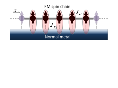
Figure 1: Graphical representation of a FM spin chain deposited on the top of a metallic surface. Kondo-screening of the individual spins at low temperatures $T\ll T_{K}$ tends to destroy the FM long-range order and induce a quantum phase transition to a paramagnetic phase (cf. Fig. 4).

The coupling between the spin chain and the metallic substrate is described by an anisotropic Kondo-exchange Hamiltonian [16]:

$$H_{K} = \sum_{i=1}^{N}J_{K}^{\perp}\left[S_{i}^{x}s^{x}\left(\mathbf{R}_{i}\right)+S_{i}^{y}s^{y}\left(\mathbf{R}_{i}\right)\right]+J_{K}^{z}S_{i}^{z}s^{z}\left(\mathbf{R}_{i}\right),$$ (2)

where $s^{a}\left(\mathbf{R}_{i}\right)$ ($a=x,y,z$) is the spin-density of conduction electrons at the position of the $i$-th spin impurity in the surface $\mathbf{R}_{i}=i.a_{0}$ (with $a_{0}$ the lattice parameter of the chain). Note that this model bears some similarity with the Kondo-lattice model, which is used to describe the properties of heavy-fermion systems [16, 33, 34]. In the case of impurities with $S>\frac{1}{2}$, the Kondo exchange involves more channels (with channel-dependent couplings) and results in a dynamical screening of the impurity spins occurring in several stages, involving different Kondo temperatures [35]. We shall not pursue such an analysis here.

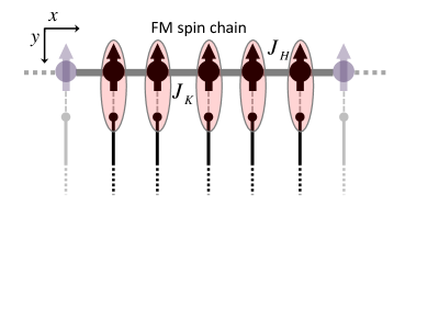
Figure 2: Local bath approximation. For impurities embedded in a 2D or 3D metallic substrate, the interference of Kondo screening clouds is negligible when the impurities are separated by a few Fermi wave numbers $k_{F}^{-1}$ [36, 37, 38], and therefore can be considered as independently screened [15].

Despite its simplicity, the model introduced above still represents a formidable theoretical challenge, and in order to make analytical progress we shall introduce some simplifying assumptions. We approximate the metallic substrate by a collection of one-dimensional metals (cf. Fig. 2) described by the Hamiltonian

$$H_{F} = \sum_{i=1}^{N}\sum_{k,\alpha}\left(\epsilon_{k}-\mu\right)\>c_{\alpha i}^{\dagger}\left(k\right)c_{\alpha i}\left(k\right),$$ (3)

where $c_{\alpha i}^{\dagger}\left(k\right)$ creates an electron with linear momentum $k$ and spin projection $\alpha$. The index $i$ indicates that the electron reservoir described by the operators $c_{\alpha i}^{{\dagger}}\left(k\right),c_{\alpha i}\left(k\right)$ is only coupled to the impurity located at $\mathbf{R}_{i}$ and not to others with $j\neq i$. For this reason, we dubbed this approximation the “local bath approximation” (LBA) [15]. Within the LBA, the spin-density operator reads:

$$s^{a}\left(\mathbf{R}_{i}\right) = \sum_{\alpha,\beta}c_{\alpha i}^{\dagger}\left(k\right)\left(\frac{\sigma^{a}}{2}\right)_{\alpha\beta}c_{\beta i}\left(k\right),$$ (4)

where $\sigma^{a}$ are the Pauli matrices.

The dimensionality of the substrate is crucial for the justification of the LBA. When the magnetic impurities embedded in a high-dimensional (2D or 3D) metallic substrate are separated by a distance of the order of a few $k_{F}^{-1}$, with $k_{F}$ the Fermi wavevector of conduction electrons, the interference of Kondo screening clouds that dynamically quench the magnetic moments, becomes negligible [36, 37, 38]. Consequently, at distances $a_{0}\gtrsim k_{F}^{-1}$ the impurities can be considered as independently screened [15]. This is an important difference with respect to the case of a strictly 1D metallic substrate, as in the case of the 1D Kondo-lattice model [39]. In that case, the single Kondo-impurity limit is reached only at distances $a_{0}\gg\xi_{K}\sim v_{F}/T_{K}$. Since the Kondo temperature $T_{K}$ is an exponentially small scale, in the purely 1D geometry the single-impurity regime is only reached at extremely dilute impurity-spin concentrations [36, 37, 38].

In actual experiments, although the magnetic nanostructures are built on the top of a metallic surface, $k_{F}$ is determined by the 3D bulk electron density due to a non-vanishing overlap between the bulk and surface conduction states [19]. For instance, the Fermi wave number for Au bulk free conduction electrons is $\pi/k_{F}^{\textrm{bulk}}=2.6\textrm{\AA}$, while for Au(111) surface states is $\pi/k_{F}^{\textrm{surf}}=16.6\textrm{\AA}$ [40]. This fact dramatically increases the range of applicability of the LBA. The physical picture provided by the LBA is also supported by the behavior of the STS Fano line shapes in experiments on magnetic Co atoms deposited on Cu$(100)$ and separated by distances $a_{0}>8\>\textrm{\AA}$, which are identical to the single-impurity STS line shapes [41].

In addition, although in the actual experimental realizations the limit $a_{0}\gg k_{F}^{-1}$ might not be strictly realized, the model resulting from applying the LBA to Eqs. (1,2) can be considered as the simplest “toy model” that captures the competition between the Kondo physics, which is a local quantum critical phenomenon, and the magnetic interactions along the chain [15]. Concerning the latter, it is worth noting that the LBA cannot reproduce the non-local RKKY exchange coupling mediated by the metal and arising at order $\mathcal{O}\left(J_{K}^{2}\right)$. As mentioned before, this is not a crucial drawback, since one can always redefine the couplings $J_{H}^{\perp},J_{H}^{z}$ in Eq. (1) to take the RKKY contribution explicitly into account. More importantly, what eventually justifies the separate treatment of RKKY and Kondo interactions is that, although they both originate in the same Hamiltonian (2), the RKKY interaction results from electronic states deep inside the Fermi sea and is a static coupling, while the Kondo effect is purely dynamical effect originated predominantly in the Fermi surface [42, 34].

3 Mean-field analysis of the $T\rightarrow 0$ phase diagram

In order to gain insight into the low-temperature phase diagram of the system, we now focus on the limit $\Delta>1$ of Eq. (1), describing an isolated FM Ising spin chain. In that case, the ground state of the isolated chain is separated from the single-magnon excitation spectrum by a gap $E_{g}=J_{H}^{z}\left(1-\Delta^{-1}\right)$ and by a gap $E_{g}^{\prime}=J_{H}^{z}\left(1-\Delta^{-2}\right)>E_{g}$ from the two-magnon bound states  [28, 29]. This means that the long-range FM order in the isolated chain is stable at low temperatures and, to a first approximation, it is safe to take $J_{H}^{\perp}=0$ in Eq. (1).

We now introduce the coupling to the substrate Eq. (2), which has important consequences for the low-temperature behavior of the the spin chain. For instance, the nature of the ferromagnetic to paramagnetic phase transition is profoundly modified. As we show in the A, in the case $J_{H}^{\perp}=0$ the model for the Ising chain coupled to the substrate can be mapped onto the 1D dissipative quantum Ising model, which is in the universality class of the classical 3D (instead of 1D) Ising model. In the following, we exploit this fact to introduce a mean-field (MF) approach, which therefore provides a good description of the phases of the spin chain in the (easy-axis) Ising limit.

We introduce the MF approximation to the Ising term in Eq. (1) by making the replacement $S_{i}^{z}S_{i+1}^{z}\rightarrow S_{i}^{z}\left\langle S_{i+1}^{z}\right\rangle+\left\langle S_{i}^{z}\right\rangle S_{i+1}^{z}-\left\langle S_{i}^{z}\right\rangle\left\langle S_{i+1}^{z}\right\rangle$, which leads to the MF Hamiltonian of the spin chain:

$$H_{0}^{MF} = \frac{Nh_{\text{eff}}^{2}}{4J_{H}^{z}}-\sum_{i=1}^{N}h_{\text{eff}}S_{i}^{z},$$ (5)

where

$$h_{\text{eff}} = 2J_{H}^{z}\left\langle S_{i}^{z}\right\rangle$$ (6)

is the local Weiss field. The MF Hamiltonian of the system is therefore written as

$$H^{MF} = \sum_{i=1}^{N}\mathcal{H}_{i}^{MF}+\frac{Nh_{\text{eff}}^{2}}{4J_{H}^{z}},$$ (7)

$$\mathcal{H}_{i}^{MF} = J_{K}^{\perp}\left[S_{i}^{x}s^{x}\left(\mathbf{R}_{i}\right)+S_{i}^{y}s^{y}\left(\mathbf{R}_{i}\right)\right]+J_{K}^{z}S_{i}^{z}s^{z}\left(\mathbf{R}_{i}\right)$$ (8)

$$-h_{\text{eff}}S_{i}^{z}+\mathcal{H}_{Fi},$$

with $\mathcal{H}_{Fi}=\sum_{k\alpha}\epsilon_{k}\>c_{\alpha i}^{\dagger}\left(k\right)c_{\alpha i}\left(k\right)$ describing the $i$-th conduction electron bath. In the following we drop the lattice sub-index $i$ in $\mathcal{H}_{i}^{MF}$ and $\mathcal{H}_{Fi}$ in order to lighten the notation.

We note that the MF approximation together with the LBA leads to a set of independent Kondo-impurity problems in an effective magnetic field $h_{\text{eff}}$, which is a quantity that must be obtained self-consistently. The MF thermodynamical properties of the spin-chain can therefore be obtained from the free-energy $f\left(T,h_{\text{eff}}\right)=-T\ln\text{Tr }\left[e^{-\mathcal{H}^{MF}\left(h_{\text{eff}}\right)/T}\right]$ for a single Kondo impurity in a magnetic field $h_{\text{eff}}$. Note that the Weiss field $h_{\mathrm{eff}}$ does not act upon the conduction electrons, it only acts on the impurity. The mean-field self-consistency condition is obtained from the relation between the impurity magnetization,

$$m_{\text{imp}}\left(T,h_{\text{eff}}\right)=\left\langle S^{z}\right\rangle=-\frac{\partial f\left(T,h_{\text{eff}}\right)}{\partial h_{\text{eff}}}$$ (9)

and the definition of the Weiss field Eq. (6):

$$m_{\text{imp}}\left(T,h_{\text{eff}}\right) = \frac{h_{\text{eff}}}{2J_{H}^{z}}.$$ (10)

To make further progress we now need to know the function $m_{\text{imp}}\left(T,h_{\text{eff}}\right)$ for a single Kondo impurity. Introducing the Abelian bosonization method [31] to describe the metallic 1D chains in Fig. 2, and the unitary Emery-Kivelson transformation [43] [cf. Eq. (48)], the anisotropic Kondo model can be mapped onto the resonant-level model [44, 45, 46]. The resonant-level model is exactly solvable when the parameter $J_{K}^{z}$ is chosen at the so-called “Toulouse line” [47], defined by $\tan^{-1}\left(\pi\rho_{0}b_{0}J_{K}^{z*}/4\right)=\frac{\pi}{2}\left(1-\frac{1}{\sqrt{2}}\right)$, where $\rho_{0}$ and $b_{0}$ are the density of states and lattice parameter of the bosonized 1D chains, respectively (cf. A). In combination with the renormalization group (RG) approach [48], which describes the flow of parameters $\left\{J_{K}^{z}\left(\ell\right),J_{K}^{\perp}\left(\ell\right)\right\}$ of the anisotropic Kondo model as a function of the conduction-band cutoff parametrized by $\Lambda\left(\ell\right)=\Lambda_{0}e^{-\ell}$, the mapping to the resonant-level model allows to describe the physical properties of the strong coupling limit of the Kondo model. One starts with the “bare” couplings $\left\{J_{K}^{z},J_{K}^{\perp}\right\}=\left\{J_{K}^{z}\left(\ell=0\right),J_{K}^{\perp}\left(\ell=0\right)\right\}$, and renormalizes up to the point where $J_{K}^{z}\left(\ell^{*}\right)=J_{K}^{z*}$, and at that point we use the exact solution of the resonant-level model [31]. However, we stress that $m_{\text{imp}}\left(T,h_{\text{eff}}\right)$ can be obtained in a more general case (and with more sophistication) using any “impurity-solver” method, such as the numerical renormalization group (NRG) [16]. The mapping to the resonant-level model yields the result [44, 45, 46]

$$m_{\text{imp}}\left(T,h_{\text{eff}}\right) = \frac{1}{\pi}\text{Im}\>\left[\psi\left(\frac{1}{2}+\frac{T_{K}}{2\pi T}+\frac{ih_{\text{eff}}}{2\pi T}\right)\right],$$ (11)

where $\psi\left(z\right)$ is the digamma function [49] and the broadening of the resonant level $\Gamma=\rho_{0}b_{0}\left(\frac{J_{K}^{\perp}\left(\ell^{*}\right)}{4\sqrt{\pi}}\right)^{2}$ can be interpreted as $T_{K}\sim\Gamma$.

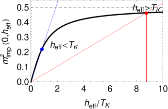
Figure 3: Graphical solution of the mean-field equation, Eq. 10, for $T=0$. For $J_{H}^{z}$ larger than the critical value there are two kinds of mean-field solutions: those for which $h_{\text{eff}}<T_{K}$ and those for which $h_{\text{eff}}>T_{K}$. In the first case, the coupling between the impurities does not suffice to destroy the Kondo singlet. However, in the latter case, the coupling is strong enough to break the Kondo singlets.

The phase boundary between the FM phase where $\left\langle S^{z}\right\rangle\propto h_{\text{eff}}\neq 0$, and the paramagnetic phase with $\left\langle S^{z}\right\rangle=0$ is obtained from (10) in the limit $h_{\text{eff}}\rightarrow 0$ (cf. Fig 3). For $\left\{T/T_{K},h_{\text{eff}}/T_{K}\right\}\ll 1$, the impurity exhibits a characteristic (Pauli) paramagnetic response $m_{\text{imp}}\left(T,h_{\text{eff}}\right)=\chi_{\text{imp}}\left(T\right)\,h_{\text{eff}}$, where

$$\chi_{\text{imp}}\left(T\right) = \frac{1}{2\pi^{2}T}\psi^{\prime}\left(\frac{1}{2}+\frac{T_{K}}{2\pi T}\right),$$ (12)

$$\approx \chi_{\text{imp}}\left(0\right)\left[1-\frac{\pi^{2}}{3}\left(\frac{T}{T_{K}}\right)^{2}+\mathcal{O}\left(\frac{T}{T_{K}}\right)^{4}\right],$$ (13)

where $\chi_{\text{imp}}\left(0\right)=1/\pi T_{K}$ is the magnetic susceptibility of the impurity at $T=0$. On the other hand, for $h_{\text{eff}}\gg\text{min}\left\{T_{K},T\right\}$, $m_{\mathrm{imp}}\left(T,h_{\text{eff}}\right)$ approaches the saturation limit of $1/2$ as

$$m_{\mathrm{imp}}\left(T,h_{\text{eff}}\right) \simeq \frac{1}{\pi}\arctan\left[\frac{h_{\text{eff}}}{2\pi T+T_{K}}\right].$$ (14)

The above result can be also obtained using the scaling equations, and it is modified by anisotropy at the Toulouse point. Thus, a non-vanishing solution for $h_{\text{eff}}$ is found from Eq. (10) in the limit $h_{\text{eff}}\rightarrow 0$

$$\frac{1}{2J_{H}^{z}} < \chi_{\text{imp}}\left(0\right)\left[1-\frac{\pi^{2}}{3}\left(\frac{T}{T_{K}}\right)^{2}\right].$$ (15)

From the above considerations, the phase boundary is therefore given by the critical line

$$\frac{T_{c}}{T_{K}} = \frac{\sqrt{3}}{\pi}\sqrt{1-\frac{\pi T_{K}}{2J_{H}^{z}}},$$ (16)

and from here we can obtain the MF phase diagram of the spin chain (See Fig. 4).

It is interesting to note that, in the FM phase, as $J_{H}^{z}/T_{K}$ increases from the phase boundary, the value of the Weiss field $h_{\mathrm{eff}}$ crosses over from a regime $h_{\mathrm{eff}}\ll T_{K}$ where the Kondo singlet is still robust, to the regime of large $h_{\mathrm{eff}}\gg T_{K}$ where the Kondo singlet is destroyed (cf. Fig. 3). Therefore, the above mean-field theory yields a regime where the Kondo effect and a FM LRO coexist. In the following Section, we shall return to this point again.

It is also worth mentioning that the result in Eq. (16) clearly contrasts with the case of the isolated Ising chain, for which the analytical form of $T_{c}$ Eq. (16), is very different from the expression for $T_{c}$ encountered in the study of the classical Ising model, where $T_{c}\propto J_{H}^{z}$ [50]. Physically, in the present case, the spin-flip processes induced by the Kondo coupling to the metal Eq. (2) can be considered as quantum fluctuations that tend to destroy the LRO in the Ising chain as $T\rightarrow 0$ for $J_{H}^{z}/T_{K}\lesssim 1.6$ (See Fig. 4).

In the following Section we characterize the excitations of the ordered FM phase.

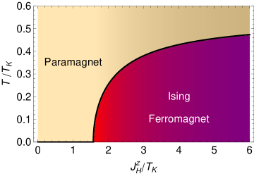
Figure 4: Mean-field phase diagram of the Ising chain coupled to the metallic substrate. At low enough temperatures, and in the regime $J_{H}^{z}\ll T_{K}$ quantum fluctuations induced by the (Kondo) coupling to the substrate completely destroy the long-range magnetic order.

4 Magnetic excitations in the FM phase

We next focus on the FM phase, in the regime $J_{H}^{z}/T_{K}\gtrsim 1$ (right-bottom region in Fig. 4), where the spectrum of the system is gapped and the effective Weiss field $h_{\text{eff}}$ is large enough so as to inhibit the Kondo screening of the impurities. We shall focus in particular on single magnon excitations that can be created by probes (such like spin-polarized electron energy loss spectroscopy, SPEELS, see Section 5) that couple weakly to the ferromagnetic chains. Such probes are assumed to produce single spin-flips, and thus the calculation of the system response can be carried out within linear response theory. This approximation allows us to neglect the effect of magnon bound states in the spectrum of the FM XXZ chain. Thus, the low-lying excitations involving a single spin-flip can be described using the Holstein-Primakoff (HP) representation of the spin operators [51]:

$$S_{i}^{+} = b_{i}^{\dagger}\sqrt{2S-b_{i}^{\dagger}b_{i}}=\sqrt{2S}\left[b_{i}^{\dagger}+O\left(\frac{1}{S}\right)\right],$$ (17)

$$S_{i}^{-} = \sqrt{2S-b_{i}^{\dagger}b_{i}}b_{i}=\sqrt{2S}\left[b_{i}+O\left(\frac{1}{S}\right)\right],$$ (18)

$$S_{i}^{z} = \left(b_{i}^{\dagger}b_{i}-S\right),$$ (19)

where $b_{i},b_{i}^{\dagger}$ are bosonic annihilation and destruction operators, obeying $\left[b_{i},b_{j}^{\dagger}\right]=\delta_{ij}$, which physically represent a single spin-flip. For the XXZ chain introduced in Sec. 2, we should take $S=\frac{1}{2}$ in the above expressions. However, below we shall work assuming that $S$ is large, which is known to provide an accurate description of the lowest energy excitations [51]. Assuming $S$ large means that our results also apply to spin chains with $S>\frac{1}{2}$, provided the Hamiltonian is of the XXZ form and we assume that the Kondo-exchange coupling with the substrate describes the strongest channel of substrate electrons that couple to each impurity along the chain. Thus, working to leading order in $S$ (i.e. in the large-$S$ approximation), we find:

$$H_{0}^{HP} \simeq \sum_{i=1}^{N}\left[-J_{H}^{z}S^{2}-J_{H}^{\perp}S\left(b_{i}^{\dagger}b_{i+1}+b_{i+1}^{\dagger}b_{i}\right)\right.$$ (20)

$$\left.+J_{H}^{z}S\left(b_{i}^{\dagger}b_{i}+b_{i+1}^{\dagger}b_{i+1}\right)\right],$$

which can be easily diagonalized in a running-wave basis

$$b_{i} = \frac{1}{\sqrt{N}}\sum_{q}e^{iqR_{i}}\>b_{q},$$ (21)

and leads to

$$H_{0}^{HP} = \sum_{q}E_{q}b_{q}^{\dagger}b_{q}-NJ_{H}^{z}S^{2}+\mathcal{O}\left(1\right),$$ (22)

where

$$E_{q} = 2SJ_{H}^{z}-2SJ_{H}^{\perp}\cos\left(qa_{0}\right),$$ (23)

$$\simeq 2S\left(J_{H}^{z}-J_{H}^{\perp}\right)+2SJ_{H}^{\perp}\frac{q^{2}a^{2}_{0}}{2}+\mathcal{O}\left(q^{4}\right),$$

is the dispersion relation for magnons, and $a_{0}$ is the lattice parameter. In addition, in Eq. (22) we have neglected terms of $\mathcal{O}\left(1\right)$, which involve interactions between the magnons. From Eq. (23), we see that for $J_{H}^{z}>J_{H}^{\perp}>0$ (i.e. $\Delta>1$) the excitation spectrum of the spin chain is gapped, and the spin waves exhibit a quadratic dispersion for momentum $q\to 0$.

Let us next consider on the Kondo-exchange coupling to the metal, Eq. (2). We shall treat this coupling using the HP representation in the large-$S$ limit:

$$H_{K}^{HP} \simeq \sum_{i=1}^{N}\left[J_{K}^{\perp}\sqrt{S/2}\left(b_{i}^{\dagger}s^{-}\left(\mathbf{R}_{i}\right)+s^{+}\left(\mathbf{R}_{i}\right)b_{i}\right)\right.$$ (24)

$$\left.+\left(b_{i}^{\dagger}b_{i}-S\right)s^{z}\left(\mathbf{R}_{i}\right)\right].$$

As we will see, although this Hamiltonian no longer describe the Kondo effect (we recall that we are working in the limit of large $h_{\text{eff}}$), the coupling to the gapless degrees of freedom in the metal still can have important consequences to the spin chain. To make further progress, we now need to integrate out the electronic degrees of freedom in the conduction band. To this end, we shall rely upon the coherent-state functional integral representation of the partition function [52]:

$$Z = \int\prod_{i=1}^{N}\mathcal{D}\left[\bar{b}_{i},b_{i}\right]\;e^{-\mathcal{S}_{\mathrm{eff}}^{HP}\left[\bar{b},b\right]},$$ (25)

where $\mathcal{S}_{\mathrm{eff}}^{HP}\left[\bar{b}_{i},b_{i}\right]$ is the effective Euclidean action of the spin chain

$$\mathcal{S}_{\mathrm{eff}}^{HP}\left[\bar{b},b\right] = \mathcal{S}_{0}^{HP}\left[\bar{b},b\right]+\mathcal{S}_{\text{diss}}^{HP}\left[\bar{b},b\right],$$ (26)

where the first term is the Euclidean action corresponding to (22)

$$\mathcal{S}_{0}^{HP}\left[\bar{b},b\right] = \sum_{q}\int_{0}^{\hbar\beta}d\tau\bar{b}_{q}\left(\tau\right)\left[\partial_{\tau}+E_{q}/\hbar\right]b_{q}\left(\tau\right),$$ (27)

$$= \frac{1}{\hbar^{2}\beta}\sum_{q,\omega_{n}}\left[-i\hbar\omega_{n}+E_{q}\right]\bar{b}_{q}\left(\omega_{n}\right)b_{q}\left(\omega_{n}\right),$$ (28)

and $\mathcal{S}_{\text{diss}}^{HP}\left[\bar{b},b\right]=-\ln\left\langle\exp\left[-\int_{0}^{\hbar\beta}d\tau\;H_{K}^{HP}\left(\tau\right)\right]\right\rangle_{Fi}$ is the contribution arising from Hamiltonian (24), where we integrate over the fermions $\left(c_{\alpha i},\bar{c}_{\alpha i}\right)$. Note that this can be done exactly, as $H_{F}$ is quadratic (we assume that Fermi liquid theory applies) and leads to

$$\mathcal{S}_{\text{diss}}^{HP}\left[\bar{b},b\right] = \frac{S}{4\hbar}\sum_{i=1}^{N}\int_{0}^{\hbar\beta}d\tau d\tau^{\prime}\,\left\{\left(J_{K}^{\perp}\right)^{2}\left[\bar{b}_{i}\left(\tau\right)\chi_{F}^{\pm}\left(\tau-\tau^{\prime}\right)b_{i}\left(\tau^{\prime}\right)\right]\right.$$ (29)

$$+\left(J_{K}^{z}\right)^{2}\left[\bar{b}_{i}\left(\tau\right)b_{i}\left(\tau\right)-S\right]\chi_{F}^{zz}\left(\tau-\tau^{\prime}\right)$$

$$\left.\times\left[\bar{b}_{i}\left(\tau^{\prime}\right)b\left(\tau^{\prime}\right)-S\right]\right\},$$

where we have introduced the spin correlation functions in the conduction band:

$$\chi_{F}^{\pm}\left(\tau\right) = -\frac{1}{\hbar}\langle s^{+}\left(\mathbf{R}_{i},\tau\right)s^{-}\left(\mathbf{R}_{i},0\right)\rangle_{F},$$ (30)

$$\chi_{F}^{zz}\left(\tau\right) = -\frac{1}{\hbar}\langle s^{z}\left(\mathbf{R}_{i},\tau\right)s^{z}\left(\mathbf{R}_{i},0\right)\rangle_{F}.$$ (31)

Note that these correlation functions do not depend on $\mathbf{R}_{i}$ because all the local fermion baths are identical. Now, since these baths are assumed to be Fermi liquids, we have that at $T=0$ and for $\tau\gg\frac{\hbar}{\epsilon_{F}}$ (where $\epsilon_{F}$ is the Fermi energy of the metallic substrate):

$$\chi_{F}^{\pm}\left(\tau\right)\sim-\frac{\lambda^{\pm}}{\tau^{2}},\quad\chi_{F}^{zz}\left(\tau\right)\sim-\frac{\lambda^{zz}}{\tau^{2}},$$ (32)

which follows from the existence of a $\sim\omega$ (where $\omega$ is the excitation energy) spectrum of particle-hole excitations in the Fermi sea at low energies. Note that since $\chi_{F}^{\pm}$ and $\chi_{F}^{zz}$ have units of $\left(E\times t\right)^{-1}$ (where $E$ and $t$ denote energy and time units, respectively), which stem from the prefactor of $\hbar$ in Eq. 30 and 31; then $\lambda^{\pm},\lambda^{zz}$ have units $t/E$ . In Fourier representation, we express (32) as:

$$\chi_{F}^{\pm}\left(\omega_{n}\right) \sim \lambda^{\pm}\left|\omega_{n}\right|,$$ (33)

$$\chi_{F}^{zz}\left(\omega_{n}\right) \sim \lambda^{zz}\left|\omega_{n}\right|,$$ (34)

where $\omega_{n}=2\pi n/\beta$ are the Matsubara frequencies, and therefore Eq. (29) becomes

$$S_{\text{diss}}^{HP}\left[\bar{b},b\right] \simeq \frac{\left(J_{K}^{\perp}\right)^{2}S\lambda^{\pm}}{4\hbar^{2}\beta}\sum_{\omega_{n}\neq 0}\sum_{i=1}^{N}|\omega_{n}|\bar{b}_{i}\left(\omega_{n}\right)b_{i}\left(\omega_{n}\right),$$ (35)

where we have dropped the last term in Eq. (29) because it amounts to a (retarded) magnon-magnon interaction. This is consistent with neglecting magnon interactions in (23). The above contribution is quadratic, and replacing it into (26) leads to the effective action

$$S_{\text{eff}}^{HP}\left[\bar{b},b\right] = -\frac{1}{\hbar^{2}\beta}\sum_{q,\omega_{n}}\left[g_{q}\left(\omega_{n}\right)\right]^{-1}\bar{b}_{q}\left(\omega_{n}\right)b_{q}\left(\omega_{n}\right),$$ (36)

where we have defined the magnon propagator [52]

$$g_{q}\left(\omega_{n}\right) = \frac{1}{i\hbar\omega_{n}-E_{q}-\alpha|\omega_{n}|},$$ (37)

with $\alpha\propto\lambda^{\pm}\left(J_{K}^{\perp}\right)^{2}$ a dimensionless parameter quantifying the dissipation caused by the conduction electrons on the spin chain. We next perform the analytic continuation to real frequencies, in order to obtain the retarded magnon propagator. Thus, replacing $i\omega_{n}\to\omega+i0^{+}$ and $|\omega_{n}|\to-i\omega$, yields

$$g_{q}^{R}\left(\omega\right)=\frac{1}{\hbar\omega-E_{q}+i\alpha\omega},$$ (38)

Thus, the pole of the propagator becomes $\hbar\omega_{q}=E_{q}\left(1+i\alpha/\hbar\right)^{-1}\simeq E_{q}-i\frac{\alpha E_{q}}{\hbar}$, for small $\alpha$, which implies that the coupling to the metal Eq. (24) induces a finite lifetime $\Gamma=\hbar\alpha^{-1}$ and damping on the magnon excitations. Physically, this happens due to the presence of gapless particle-hole excitations in the excitation spectrum of the metallic substrate, and it can be interpreted as Landau damping [53, 54, 55]. Interestingly, this damping does not vanish in the limit $q\to 0$. At first sight, this may seem surprising, since in the $q\to 0$ limit, magnon excitations correspond to a uniform magnetization along the $z$ direction. Thus, the total projection of the spin along $z$, i.e., $S_{T}^{z}=\sum_{i=1}^{N}S_{i}^{z}$, is a conserved quantity in the absence of coupling to the substrate. In other words, the number of magnons $\sum_{q}b_{q}^{{\dagger}}b_{q}$ is a conserved quantity of Hamiltonian in (20). However, in the presence of $H_{K}^{HP}$ [Eq. (24)], $S_{T}^{z}$ is no longer conserved (i.e. the magnons $b_{i}$ can “leak out” from the chain), and therefore total magnetization fluctuations also become damped out by the coupling to the substrate.

The above treatment is valid provided the coupling to the substrate is weak and can be treated perturbatively. At stronger coupling, we have to worry about the possibility that the magnetic moments of the impurities are Kondo-screened by the substrate electrons. To deal with this situation, we shall rely on the non-perturbative treatment discussed in the A. As shown there, in the strong-coupling limit where Kondo correlations are important, it is possible to map the model introduced in Section 2 to a dissipative quantum Ising model. When coarse-grained over distances $\gg a_{0}$, this model can be described by a dissipative $\phi^{4}$ field theory, whose partition function is $Z=\int\left[d\phi\right]\,e^{-\mathcal{S}\left[\phi\right]}$, where the action $\mathcal{S}\left[\phi\right]$ is given by the expression [11]:

$$\mathcal{S}\left[\phi\right]=\frac{1}{2}\sum_{q,\omega_{n}}\left[\left|\omega_{n}\right|+Dq^{2}+r\right]\left|\phi\left(q,\omega_{n}\right)\right|^{2}+\frac{g}{4}\int dxd\tau\,\phi^{4}\left(x,\tau\right),$$ (39)

being $\phi\left(x,\tau\right)=\left(L\hbar\beta\right)^{-1/2}\sum_{q,\omega_{n}}\phi\left(q,\omega_{n}\right)\>e^{i\left(qx-\omega_{n}\tau\right)}$ ($\beta=1/T$) is the coarse-grained magnetization along the easy axis, i.e. $\left\langle\phi\left(x=x_{i}\right)\right\rangle=R^{-1}\sum_{j=-R/2}^{R/2}\left\langle S_{i+j}^{z}\right\rangle$, where $1\ll R\ll N$. This result suggests that the quantum critical point (QPC) separating the paramagnetic and ferromagnetic ground states (cf. Fig 4) can be described by this field theory, and therefore the critical exponents around the QCP will correspond to those of the Wilson-Fisher fixed-point of the renormalization group (see e.g. Ref. [56], for a survey). However, in deriving the map to the dissipative quantum Ising model, we have neglected the Heisenberg term $\sim\frac{J_{H}^{\perp}}{2}\sum_{i}\left[S_{i}^{+}S_{i+1}^{-}+\mathrm{H.c.}\right]$ from Eq. (1). If this term is included, we cannot rule out that the actual values of the critical exponents near the QCP turn out to be different from those of the Wilson-Fisher universality class. Addressing this question in detail require a numerical investigation of the full model, which is beyond the scope of the present work.

Nevertheless, the field theory of Eq. (39), is capable of describing the phases of the system. Focusing on the ferromagnetic phase where $\left\langle\phi\left(x,\tau\right)\right\rangle\neq 0$, which corresponds to $r<0$, it can be seen that the magnon excitations are indeed described by the propagator:

$$\left\langle\phi^{*}\left(q,\omega_{n}\right)\phi\left(q,\omega_{n}\right)\right\rangle=\frac{1}{\left|\omega_{n}\right|+Dq^{2}+E_{g}},$$ (40)

where $E_{g}=2\left|r\right|\sim J_{H}^{z}-J_{H}^{\perp}$ is the energy gap. This magnon propagator indicates that the magnetic excitations of the chain in the strong coupling regime are overdamped by their coupling to the metallic substrate. Physically, this makes sense as the impurity spins are screened by the metal electrons and thus their magnetic moments undergo strong damping by the collective nature of their screening clouds. This regime must be contrasted with the weak-coupling regime, where we found the damping to be weak. Thus, a physical picture emerges that allows us to distinguish the two mean-field solutions that we briefly described at the end of Section 3 (cf. Fig. 3): In the weak coupling regime, the strong Weiss field (i.e. $h_{\mathrm{eff}}\gg T_{K}$) due to the FM coupling of the impurities along the chain does not allow for the Kondo screening of the local moments of the atoms in the chain. As a consequence, the magnetic excitations of the chain are only weakly affected by their coupling to the substrate, and thus acquire a small line-width . On the other hand, in the strong coupling regime, the Weiss field is much weaker (i.e. $h_{\mathrm{eff}}\ll T_{K}$) and the magnetic moments are effectively screened by the metal electrons, leading to overdamped magnetic excitations. In the next Section, we shall study some experimental consequences of our findings.

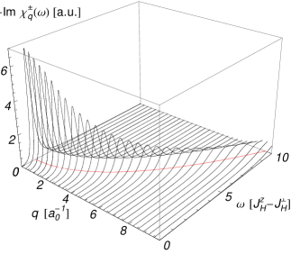
Figure 5: Spin-response $\text{Im }\chi_{q}^{\pm}\left(\omega\right)$ as a function of $q$ and $\omega$. This quantity is proportional to the SPEELS $d^{2}P/d\Omega d\omega$ signal and provides information about the magnon dispersion relation (red line in the bottom $q-\omega$ plane) and the FM Ising gap. The broadening of the magnon excitation is originated in the (Kondo) coupling to the metallic substrate Eq. (2).

5 Relation to SPEELS experiments

In this Section, we focus on the effects of the dissipative environment on observable quantities. The magnetic properties of low dimensional spin systems deposited on metals have been studied with a variety of experimental techniques, like X-ray magnetic circular dichroism (XMCD), used to measure directly the magnetization of FM 1D spin chains [22], or local probes, like spin polarized STM, which can provide information on the magnon dispersion relation [57]. Here we focus on the spin-polarized electron energy-loss spectroscopy (SPEELS) experiment [58, 59, 60], which provides direct information of the magnon dispersion relation.

The SPEELS cross section $d^{2}P/d\Omega d\omega$ corresponds to the fractional number of electrons which emerge onto the solid angle $d\Omega$ after being scattered by a magnetic excitation $\omega\left(\mathbf{q}\right)$ in the energy range $d\omega$. According to the theory of the SPEELS experiment [58], $d^{2}P/d\Omega d\omega$ is related to the spin response function by

$$\frac{d^{2}P}{d\Omega d\omega} \propto -\text{Im }\chi_{\mathbf{q}}^{\pm}\left(\omega\right),$$ (41)

where $\chi_{\mathbf{q}}^{\pm}\left(\omega\right)$ is the retarded spin correlation function obtained by analytic continuation from $\chi_{\mathbf{q}}^{\pm}\left(\omega\right)=\left[\chi_{\mathbf{q}}^{\pm}\left(\omega_{n}\right)\right]_{\omega_{n}\rightarrow\omega+i0^{+}}$with

$$\chi_{\mathbf{q}}^{\pm}\left(\omega_{n}\right) = \int d^{3}\mathbf{R}\int d\tau\;e^{i\mathbf{q.R}}e^{-i\omega_{n}\tau}\left\langle S^{-}\left(\mathbf{R},\tau\right)S^{+}\left(0,0\right)\right\rangle.$$ (42)

Using the HP representation Eqs. (17)-(19), we can express

$$\chi_{q}^{\pm}\left(\omega_{n}\right) \approx 2S\left\langle b_{q}\left(\omega_{n}\right)\bar{b}_{q}\left(\omega_{n}\right)\right\rangle,$$ (43)

$$= \frac{2S}{i\hbar\omega_{n}-\alpha|\omega_{n}|-E_{q}},$$ (44)

where we have used Eqs. (36) and (37), and the fact that in the 1D geometry $\mathbf{q}\rightarrow q$. Introducing this result into Eq. (41) and performing the analytic continuation to real frequencies, we obtain:

$$\text{Im }\chi_{q}^{\pm}\left(\omega\right)=-\frac{\alpha\omega}{\left(\hbar\omega-E_{q}\right)^{2}+\alpha^{2}\omega^{2}}.$$ (45)

In Fig. (5) we show the spin response function $-\text{Im }\chi_{q}^{\pm}\left(\omega\right)$ as a function of $q$ and $\omega$. The curves $-\text{Im }\chi_{q}^{\pm}\left(\omega\right)$ show resonances centered at the magnon frequencies $\omega=E_{q}$ (red line in the bottom $q-\omega$ plane), which are broadened by the effect of $\alpha$, the dimensionless coupling to the metal.

6 Conclusions and Outlook

We have studied the phase diagram and the excitation spectrum of a magnetic chain of atoms or molecules with easy-axis ferromagnetic interactions. We focused on a simple model of $S=\frac{1}{2}$ magnetic impurities displaying a Kondo-exchange interaction with the substrate. In the Ising limit, which provides a good approximation to the ground state of an easy-axis ferromagnet, we obtained the phase diagram using a mean-field theory approach. We find that this system exhibits two possible phases at zero temperature: a paramagnetic phase where the impurity spins are screened by the substrate, and a gapped ferromagnetic phase whose excitations are damped by the magnetic (Kondo) exchange with the metallic substrate. Using a bosonic representation for the spins as well as various types of mathematical mappings between models, we have also investigated the excitation spectrum in the ferromagnetic phase, which may be accessible through probes like spin-polarized electron energy loss (SPEELS). Although we have focused mainly on an easy-axis ferromagnetic (FM) chain, it is worth describing how our results can be modified in the case of the anti-ferromagnetic (AFM) chain corresponding to the parameter regime $\Delta<-1$ of the XXZ chain described by Eq. (1). An experimental motivation to extend our results to this regime can be found, for instance, in Ref. [24]. Relying on the local bath approximation (LBA) and in the Ising limit, it is possible to apply the transformation $S_{i}^{z}\to\left(-1\right)^{i}S_{i}^{z}$, which maps the AFM to onto FM Ising chain. In presence of the Kondo exchange, this transformation must be supplemented by another rotation which takes $s_{c}^{z}\left(\mathbf{R}_{i}\right)\to\left(-1\right)^{i}s_{c}^{z}\left(\mathbf{R}_{i}\right)$ and $s^{x}\left(\mathbf{R}_{i}\right)\leftrightarrow s^{y}\left(\mathbf{R}_{i}\right)$ provided that $(-1)^{i}=-1$. For $\Delta<-1$, the excitations are separated from the ground state by a gap $\sim\sqrt{\left(J_{H}^{z}\right)^{2}-\left(J_{H}^{\perp}\right)^{2}}$. Using the Holstein-Primakoff representation [51], we can compute the spectrum of an antiferromagnetic XXZ chain, which yields $E_{q}^{\text{AFM}}=2S\sqrt{\left(J_{H}^{z}\right)^{2}-\left(J_{H}^{\perp}\cos qa_{0}\right)^{2}}$. The results of Sections 4 and 5 carry over to the AFM ($\Delta<-1$) case provided we replace $E_{q}$ by $E_{q}^{\text{AFM}}$. A feature of the AFM regime that is also worth noticing is that bound states of magnons are absent from the spectrum [28, 29].

Finally, let us discuss our outlook for future research directions. One such direction is the study of the phases of chains of impurities with higher (i.e. $S>\frac{1}{2}$) spin. In this case, it is also possible to apply the same mean-field theory employed in Section 3. However, in order to obtain the impurity magnetization $m_{\text{imp}}\left(h_{\text{eff}},T\right)=\langle S^{z}\rangle$ we must in general resort to an impurity solver such as Wilson’s numerical renormalization group [20, 16]. This is specially true for $S>\frac{1}{2}$, which will will undergo a several stage Kondo effect [16, 35] and possibly underscreening [61]. Another interesting direction will be to asses the accuracy of the local bath approximation employed throughout. This remains quite a challenge, which will most likely require to rely on numerical methods, such as quantum Monte Carlo. Indeed, it is possible that this approximation only provides an rough picture of the paramagnetic phase, which must be corrected by the inclusion of the coupling between the different baths that screen the magnetic impurities individually. However, we believe that such effects will be less important in the ferromagnetic phase (specially for large $J_{H}^{z}$), due to the existence of a gap that separates the ferromagnetic ground state from the excitations and therefore protects the ground state from perturbations.

Appendix A Bosonization of the fermionic chains and mapping to the dissipative quantum Ising model

In this Appendix, we implement the Abelian bosonization approach to the semi-infinite fermionic 1D chains along the $y$ direction in Fig. (2) [31, 62]. This procedure is standard and has been successfully applied to describe the low-energy properties of the single Kondo-impurity. We refer the reader to the standard bibliography [31, 62, 44, 43, 63, 64]. In the present case, the LBA greatly simplifies the complexity of the problem and enables a straightforward generalization to the case of many-impurities, each one coupled to an independent fermionic bath. At low temperature, in the bosonic representation [64] the Hamiltonians (3) and (2) become

$$H_{F} = \sum_{i,\nu=\left\{c,s\right\}}\frac{v_{F}}{4\pi}\int_{-\infty}^{\infty}dy\;\left(\nabla\phi_{i,\nu}^{R}\left(y\right)\right)^{2},$$ (46)

$$H_{K} = \sum_{i}-\frac{2\delta_{s}}{\pi\rho_{0}}S_{i}^{z}\frac{\nabla\phi_{i,s}^{R}\left(0\right)}{\sqrt{2}\pi}$$ (47)

$$+\frac{J_{K}^{\perp}b_{0}}{2}\left[S_{i}^{+}\frac{e^{-i\sqrt{2}\phi_{i,s}^{R}\left(0\right)}}{2\pi b_{0}}+S_{i}^{-}\frac{e^{i\sqrt{2}\phi_{i,s}^{R}\left(0\right)}}{2\pi b_{0}}\right],$$

where $\phi_{i,c}^{R}\left(y\right),\phi_{i,s}^{R}\left(y\right)$ are bosonic chiral fields which obey the commutation relations $\left[\phi_{i,\nu}^{R}\left(y\right),\phi_{j,\eta}^{R}\left(y^{\prime}\right)\right]=i\pi\text{sign}\left(y-y^{\prime}\right)\delta_{i,j}\delta_{\nu,\eta}$, and which are related to charge and spin density-fluctuations in the 1D fermionic chains through the relations $\rho_{i}\left(y\right)=-\frac{1}{\pi}\nabla\phi_{i,c}^{R}\left(y\right)$ and $s_{i}\left(y\right)=-\frac{1}{\pi}\nabla\phi_{i,s}^{R}\left(y\right)$, respectively [31, 64]. In Eq. (46) $v_{F}$ is the Fermi velocity, and in Eq. (47) $\delta_{s}=\tan^{-1}\left(\pi\rho_{0}J_{K}^{z}b_{0}/4\right)$ is the scattering phase-shift associated with the potential $J_{K}^{z}S_{i}^{z}/2$, $\rho_{0}=\left(2\pi v_{F}\right)^{-1}$ the conduction electron density of states at the Fermi energy, and $b_{0}$ the lattice parameter in the fermionic chain. For simplicity we assume these parameters to be identical for all chains. We then introduce the (Emery-Kivelson) unitary transformation [43]

$$\mathcal{U} = \exp\left[-i\gamma\sum_{i}S_{i}^{z}\phi_{i,s}^{R}\left(0\right)\right],$$ (48)

under which the bosonic field $\nabla\phi_{i,s}^{R}\left(y\right)$ and the spin operator $S_{i}^{+}$ transform as

$$\mathcal{U}^{\dagger}\nabla\phi_{i,s}^{R}\left(y\right)\mathcal{U} = \left[\nabla\phi_{i,s}^{R}\left(y\right)+\delta\left(y\right)2\pi\gamma S_{i}^{z}\right],$$ (49)

$$\mathcal{U}^{\dagger}S_{i}^{+}\mathcal{U} = S_{i}^{+}e^{i\gamma\phi_{i,s}^{R}\left(0\right)}.$$ (50)

Upon this transformation, the total Hamiltonian of the spin-chain coupled to the metallic bath, $H=H_{0}+H_{K}+H_{F}$, transforms as $\tilde{H}=\mathcal{U}^{\dagger}H\mathcal{U}=\tilde{H}_{0}+\tilde{H}_{K}+\tilde{H}_{F}$, with

$$\tilde{H}_{0} = -\sum_{i}\left\{J_{H}^{z}S_{i}^{z}S_{i+1}^{z}\right.$$ (51)

$$\left.+\frac{J_{H}^{\perp}}{2}\left[e^{i\gamma\left[\phi_{i,s}^{R}\left(0\right)-\phi_{i+1,s}^{R}\left(0\right)\right]}S_{i}^{+}S_{i+1}^{-}+\text{H.c.}\right]\right\},$$

$$\tilde{H}_{K} = \sum_{i}\left\{-\frac{2\tilde{\delta}_{s}}{\pi\rho_{0}}S_{i}^{z}\frac{\nabla\phi_{i,s}^{R}\left(0\right)}{\sqrt{2}\pi}\right.$$ (52)

$$\left.+\frac{J_{K}^{\perp}b_{0}}{2}\left[S_{i}^{+}\frac{e^{-i\left(\sqrt{2}-\gamma\right)\phi_{i,s}^{R}\left(0\right)}}{2\pi b_{0}}+\text{H.c.}\right]\right\},$$

$$\tilde{H}_{F} = H_{F},$$ (53)

where we have defined $\tilde{\delta}_{s}\equiv\delta_{s}-\pi\gamma/2\sqrt{2}$. Note that the local bath approximation Eq. (3) is crucial to implement bosonization along the chains, and to put these ideas on a clear mathematical framework. It is also interesting to note that in the transformed representation, the quantum dynamics of the bath [represented by the chiral field $\phi_{i,s}^{R}\left(0\right)$] appears explicitly in the Heisenberg term $\sim-J_{H}^{\perp}\left(S_{i}^{+}S_{i+1}^{-}e^{i\gamma\left[\phi_{i,s}^{R}\left(0\right)-\phi_{i+1,s}^{R}\left(0\right)\right]}+\text{H.c.}\right)$ [15]. Physically, this means that the Heisenberg interaction is now “dressed” by the spin-density fluctuations of the electron gas. In the case of an easy-axis spin chain in Ising limit $J_{H}^{z}\gg J_{H}^{\perp}$, the effect of this term is negligible and can be ignored in a first approximation.

We now exploit the freedom to choose $\gamma$ and set $\gamma=\sqrt{2}$. In this case, the Hamiltonian reads

$$\tilde{H} = \tilde{H}_{0}+\tilde{H}_{K}+\tilde{H}_{F}$$ (54)

$$\simeq \sum_{i}\left[J_{H}^{z}S_{i}^{z}S_{i+1}^{z}-\frac{2\tilde{\delta}_{s}}{\pi\rho_{0}}\frac{\nabla\phi_{i,s}^{R}\left(0\right)}{\sqrt{2}\pi}S_{i}^{z}+\frac{J_{K}^{\perp}}{2\pi}S_{i}^{x}\right]+H_{F},$$

This Hamiltonian corresponds to the 1D dissipative quantum Ising model (DQIM), where now the Kondo Hamiltonian $\tilde{H}_{K}$ is equivalent to the spin-boson model with Ohmic dissipation [63, 5, 4, 14] with $\tilde{\delta}_{s}$ related to the dissipative parameter $\alpha$ in the context of macroscopic quantum coherence through $\alpha=\left(2\tilde{\delta}_{s}/\pi\right)^{2}$, and with the in-plane Kondo interaction playing the role of a magnetic field along the $x-$axis $h_{x}=-J_{K}^{\perp}/2\pi$. At $T=0$, the 1D DQIM is known to display a paramagnetic to ferromagnetic quantum phase transition which is in the universality class of quantum dissipative systems and whose dynamical critical exponent is $z=2$ [11]. Note that this is very different with the case of the 1D quantum Ising chain, which is in the universality class of the 2D classical Ising model and where $z=1$. The critical properties of this model near the quantum phase transition have been studied in the context of antiferromagnetic instabilities of Fermi liquids [56, 11] using the framework of the Hertz-Moriya-Millis theory [65, 66, 67] This theory describes critical quantum fluctuations of the order parameter around the Gaussian fixed point of the theory. The predicted value of the critical dynamical exponent $z=2$ and has been confirmed numerically with Monte Carlo simulations [12, 13]. Physically speaking, such a dynamical exponent implies that the effective dimensionality of the 1D spin chain coupled to the metallic bath is $d_{\text{eff}}=1+z=3$, and therefore fluctuations of the order parameter are expected to be much less important than the case of the non-dissipative classical or quantum Ising model. This fact supports our MF approximation, which allows to extend these results to $T>0$.

References

- [1] Roland Wiesendanger. Spin mapping at the nanoscale and atomic scale. Rev. Mod. Phys., 81(4):1495–1550, Nov 2009.
- [2] Carlo Carbone, Sandra Gardonio, Paolo Moras, Samir Lounis, Marcus Heide, Gustav Bihlmayer, Nicolae Atodiresei, Peter Heinz Dederichs, Stefan Blügel, Sergio Vlaic, Anne Lehnert, Safia Ouazi, Stefano Rusponi, Harald Brune, Jan Honolka, Axel Enders, Klaus Kern, Sebastian Stepanow, Cornelius Krull, Timofey Balashov, and Pietro Mugarza, Aitor Gambardella. Adv. Funct. Mater., 21:1212, 2011.
- [3] N. V. Prokof’ev and P. C. E. Stamp. Rep. Prog. Phys., 63:669, 2000.
- [4] U. Weiss. Quantum Dissipative Systems (2nd edition), volume 10. World Scientific Publishing Co. Pte. Ltd., Singapore, 1999.
- [5] A. J. Leggett, S. Chakravarty, A. T. Dorsey, M. P. A. Fisher, A. Garg, and W. Zwerger. Rev. Mod. Phys., 59:1, 1987.
- [6] A. O. Caldeira and A. J. Leggett. Influence of dissipation on quantum tunneling in macroscopic systems. Phys. Rev. Lett., 46(4):211–214, Jan 1981.
- [7] Sudip Chakravarty. Phys. Rev. Lett., 49:681, 1982.
- [8] A. J. Bray and M. A. Moore. Phys. Rev. Lett., 49:1545, 1982.
- [9] A. Schmid. Phys. Rev. Lett., 51:1506, 1983.
- [10] A. H. Castro Neto, C.deC. Chamon, and C. Nayak. Phys. Rev. Lett., 79:4629, 1997.
- [11] Sergey Pankov, Serge Florens, Antoine Georges, Gabriel Kotliar, and Subir Sachdev. Phys. Rev. B, 69:054426, 2004.
- [12] Philipp Werner, Klaus Völker, Matthias Troyer, and Sudip Chakravarty. Phys. Rev. Lett., 94:047201, 2005.
- [13] Philipp Werner, Matthias Troyer, and Subir Sachdev. J. Phys. Soc. Jpn., 74:67, 2005.
- [14] Peter P. Orth, Ivan Stanic, and Karyn Le Hur. Phys. Rev. A, 77:051601, 2008.
- [15] Alejandro M. Lobos, Miguel A. Cazalilla, and Piotr Chudzinski. Phys. Rev. B, 86:035455, 2012.
- [16] A. C. Hewson. The Kondo Problem to Heavy Fermions. Cambridge University Press, Cambridge, 1993.
- [17] Jiutao Li, Wolf-Dieter Schneider, Richard Berndt, and Bernard Delley. Phys. Rev. Lett., 80:2893–2896, 1998.
- [18] V. Madhavan, W. Chen, T. Jamneala, M. F. Crommie, and N. S. Wingreen. Science, 280:567, 1998.
- [19] N. Knorr, M. A. Schneider, L. Diekhoner, P. Wahl, and K. Kern. Phys. Rev. Lett., 88:096804, 2002.
- [20] Ralf Bulla, Theo A. Costi, and Thomas Pruschke. Numerical renormalization group method for quantum impurity systems. Rev. Mod. Phys., 80:395–450, Apr 2008.
- [21] A. Georges, G. Kotliar, W. Krauth, and M. J. Rozenberg. Rev. Mod. Phys., 68, 1996.
- [22] P. Gambardella, A. Dallmeyer, K. Maiti, M. C. Malagoli, W. Eberhardt, K. Kern, and C. Carbone. Nature, 416:301, 2002.
- [23] Cyrus F. Hirjibehedin, Christopher P. Lutz, and Andreas J. Heinrich. Science, 312:1021, 2006.
- [24] Andrew DiLullo, Shih-Hsin Chang, Nadjib Baadji, Kendal Clark, Jan-Peter Klöckner, Marc-Heinrich Prosenc, Stefano Sanvito, Roland Wiesendanger, and Saw-Wai Hoffmann, Germarand Hla. Nano Lett., 12:3174, 2012.
- [25] Sebastian Loth, Susanne Baumann, Christopher P. Lutz, D. M. Eigler, and Andreas J. Heinrich. Science, 335:196, 2012.
- [26] Stefan Müllegger, Mohammad Rashidi, Michael Fattinger, and Reinhold Koch. 2012.
- [27] Nader Zaki, Chris A. Marianetti, Danda P. Acharya, Percy Zahl, Peter Sutter, Junichi Okamoto, Peter D. Johnson, Andrew J. Millis, and Richard M. Osgood. Spin-exchange-induced dimerization of an atomic 1-d system. 2012.
- [28] T. Schneider and E. Stoll. Excitation spectrum of the ferromagnetic ising-heisenberg chain at zero field. Phys. Rev. B, 25:4721, 1982.
- [29] Daniel C. Mattis. The Theory of Magnetism I. Statics and Dynamics, 2nd Edition. Springer-Verlag, 1988.
- [30] E. Brezin and J. Zinn-Justin, editors. Fields, Strings and Critical Phenomena, Amsterdam, 1988. Elsevier Science Publishers.
- [31] T. Giamarchi. Quantum Physics in One Dimension. Oxford University Press, Oxford, 2004.
- [32] M. A. Ruderman and C. Kittel. Phys. Rev., 96:66, 1954.
- [33] H.V. Löhneysen. J. Magn. Magn. Mat., 200:532, 1999.
- [34] Quimiao Si and Frank Steglich. Science, 329, 2010.
- [35] P. Nozières and A. Blandin. J. Phys. (Paris), 41:193, 1980.
- [36] Lucio Claudio Andreani and Hans Beck. Phys. Rev. B, 48:7322–7337, 1993.
- [37] Victor Barzykin and Ian Affleck. Phys. Rev. B, 61:6170, 2000.
- [38] J. Simonin. cond-mat/0708.3604, 2007.
- [39] O. Zachar, S. A. Kivelson, and V. J. Emery. Exact results for a 1d kondo lattice from bosonization. Phys. Rev. Lett., 77:1342, 1996.
- [40] O. Újsághy, J. Kroha, Szunyogh, and A. Zawadowski. Phys. Rev. Lett., 85:2557, 2000.
- [41] P. Wahl, P. Simon, L. Diekhöner, V. S. Stepanyuk, P. Bruno, M. A. Schneider, and K. Kern. Exchange interaction between single magnetic adatoms. Phys. Rev. Lett., 98(5):056601, Jan 2007.
- [42] A. H. Castro Neto and B. A. Jones. Phys. Rev. B, 62:14975–15011, 2000.
- [43] V. J. Emery and S. A. Kivelson. In H. van Beijeren and M. E. Ernst, editors, Fundamental Problems in Statistical Mechanics VII: Proceedings of the 1993 Altenberg Summer School, Amsterdam, 1994. North Holland.
- [44] P. Schlottmann. J. Phys. (Paris), C6:1486, 1978.
- [45] P. B. Wiegmann and A. M. Finkelshtein. Sov. Phys. JETP, 48:102, 1978.
- [46] A. M. Tsvelick and P. B. Wiegmann. Adv. Phys., 32:453, 1983.
- [47] G. Toulouse. C. R. Acad. Sci. B, 268:1200, 1969.
- [48] P. W. Anderson, G. Yuval, and D. R. Hamann. Phys. Rev. B, 1:4464, 1970.
- [49] M. Abramowitz and I. Stegun. Handbook of mathematical functions. Dover, New York, 1972.
- [50] N. W. Ashcroft and N. D. Mermin. Solid State Physics. Saunders College, Philadelphia, 1976.
- [51] A. Auerbach. Interacting Electrons and Quantum Magnetism. Springer, Berlin, 1998.
- [52] J.W. Negele and H. Orland. Quantum Many Particle systems. Frontiers in Physics. Addison-Wesley, Reading, Mass., 1987.
- [53] A. T. Costa, R. B. Muniz, and D. L. Mills. Theory of spin excitations in fe(110) multilayers. Phys. Rev. B, 68:224435, 2003.
- [54] A. T. Costa, R. B. Muniz, and D. L. Mills. Theory of spin waves in ultrathin ferromagnetic films: The case of co on cu(100). Phys. Rev. B, 69:064413, Feb 2004.
- [55] Paweł Buczek, Arthur Ernst, and Leonid M. Sandratskii. Interface electronic complexes and landau damping of magnons in ultrathin magnets. Phys. Rev. Lett., 106:157204, 2011.
- [56] Subir Sachdev. Quantum Phase Transitions. Cambridge University Press, Cambridge, UK, 2000.
- [57] T. Balashov, A. F. Takács, W. Wulfhekel, and J. Kirschner. Magnon excitation with spin-polarized scanning tunneling microscopy. Phys. Rev. Lett., 97:187201, 2006.
- [58] M. P. Gokhale, A. Ormeci, and D. L. Mills. Phys. Rev. B, 46:8978–8993, 1992.
- [59] J. Prokop, W. X. Tang, Y. Zhang, I. Tudosa, T. R. F. Peixoto, Kh. Zakeri, and J. Kirschner. Magnons in a ferromagnetic monolayer. Phys. Rev. Lett., 102:177206, 2009.
- [60] Y. Zhang, P. A. Ignatiev, J. Prokop, I. Tudosa, T. R. F. Peixoto, W. X. Tang, Kh. Zakeri, V. S. Stepanyuk, and J. Kirschner. Elementary excitations at magnetic surfaces and their spin dependence. Phys. Rev. Lett., 106:127201, Mar 2011.
- [61] P. Mehta, N. Andrei, P. Coleman, L. Borda, and G. Zaránd. Regular and singular fermi-liquid fixed points in quantum impurity models. Phys. Rev. B, 72:014430, 2005.
- [62] A. O. Gogolin, A. A. Nersesyan, and A. M. Tsvelik. Bosonization and Strongly Correlated Systems. Cambridge University Press, Cambridge, 1999.
- [63] F. Guinea, V. Hakim, and A. Muramatsu. Phys. Rev. B, pages 4410–4418, 1985.
- [64] Gabriel Kotliar and Qimiao Si. Phys. Rev. B, 53:12373–12388, 1996.
- [65] John A. Hertz. Phys. Rev. B, 14:1165, 1976.
- [66] T. Moriya and J. Kawabata. J. Phys. Soc. Jpn., 34:639, 1973.
- [67] A. J. Millis. Phys. Rev. B, 48:7183–7196, 1993.