Lattice measurement of ฮฑssubscript๐›ผ๐‘ \alpha_{s} with a realistic charm quark

B.ย Blossier benoit.blossier@th.u-psud.fr Ph.ย Boucaud M.ย Brinet F.ย De Soto X.ย Du V.ย Morรฉnas O.ย Pรจne K.ย Petrov J.ย Rodrรญguez-Quintero Laboratoire de Physique Thรฉorique, Universitรฉ de Paris XI, Bรขtiment 210, 91405 Orsay Cedex, France Laboratoire de Physique Subatomique et de Cosmologie, CNRS/IN2P3/UJF; 53, avenue des Martyrs, 38026 Grenoble, France Dpto. Sistemas Fรญsicos, Quรญmicos y Naturales, Univ. Pablo de Olavide, 41013 Sevilla, Spain Laboratoire de Physique Corpusculaire, Universitรฉ Blaise Pascal, CNRS/IN2P3 63177 Aubiรจre Cedex, France Laboratoire de lโ€™Accรฉlรฉrateur Linรฉaire โ€“ IN2P3/CNRS, Centre Scientifique dโ€™Orsay, Bรขtiment 200 โ€“ BP 34, 91898 Orsay Cedex, France Dpto. Fรญsica Aplicada, Fac. Ciencias Experimentales; Universidad de Huelva, 21071 Huelva; Spain
Abstract

We report on an estimate of ฮฑssubscript๐›ผ๐‘ \alpha_{s}, renormalised in the $\overline{MS}$ scheme at the $\tau$ and $Z^{0}$ mass scales, by means of lattice QCD. Our major improvement compared to previous lattice calculations is that, for the first time, no perturbative treatment at the charm threshold has been required since we have used statistical samples of gluon fields built by incorporating the vacuum polarisation effects of $u/d$, s๐‘ s and $c$ sea quarks. Extracting ฮฑssubscript๐›ผ๐‘ \alpha_{s} in the Taylor scheme from the lattice measurement of the ghost-ghost-gluon vertex, we obtain ฮฑsMSยฏโ€‹(mZ2)=0.1200โ€‹(14)subscriptsuperscript๐›ผยฏMS๐‘ subscriptsuperscript๐‘š2๐‘0.120014\alpha^{\rm\overline{MS}}_{s}(m^{2}_{Z})=0.1200(14) and ฮฑsMSยฏโ€‹(mฯ„2)=0.339โ€‹(13)subscriptsuperscript๐›ผยฏMS๐‘ subscriptsuperscript๐‘š2๐œ0.33913\alpha^{\rm\overline{MS}}_{s}(m^{2}_{\tau})=0.339(13).

โ€ โ€ journal: Nuc. Phys. (Proc. Suppl.)

1 Introduction

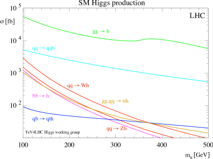
The recent announcement by ATLAS and CMS of their observation at 5 $\sigma$ significance of a new particle with a mass around 125 GeV [1], interpreted as the Brout-Englert-Higgs (BEH) boson, makes even more crucial than before a satisfying control on theoretical inputs of analytical expression of the Higgs decay channels. Indeed, the era of precise Higgs physics (measurement of the couplings, โ€ฆ) will certainly open soon: assessing the sensitivity of forthcoming detectors will be a key ingredient. There are different modes of Higgs boson production: however the gluon-gluon fusion is by far the dominant process, as shown in Fig.ย 1. Over the uncertainty $\Delta\sigma^{\rm th}_{gg\to H\to X}$ of 20 - 25 % claimed at LHC ($\sqrt{s}=7\,{\rm TeV})$, about 4 % come from the uncertainty ฮดโ€‹ฮฑs๐›ฟsubscript๐›ผ๐‘ \delta\alpha_{s} on ฮฑsโ€‹(mZ02)subscript๐›ผ๐‘ subscriptsuperscript๐‘š2superscript๐‘0\alpha_{s}(m^{2}_{Z^{0}}) [2]. A complementary approach of the ฮฑssubscript๐›ผ๐‘ \alpha_{s} measurement from the analysis of Deep Inelastic Scattering data, physics of jets, $\tau$ decay and $e^{+}e^{-}\to$ hadrons [3] is its computation by numerical simulations. In the following section we will report on the work performed by the ETM Collaboration to measure ฮฑssubscript๐›ผ๐‘ \alpha_{s} from $N_{f}=2+1+1$ gauge configurations [4].

Refer to caption

Figure 1: Prediction of the Standard Model BEH boson production in function of its mass for different production channels at LHC

2 ฮฑssubscript๐›ผ๐‘ \alpha_{s} from numerical simulations

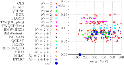
In the past years tremendous progresses have been made by the lattice community to perform simulations that are closer to the physical point. It means including more and more quark species in the sea, $u/d$ quarks $(N_{f}=2)$, then the strange $(N_{f}=2+1)$ and even the charm $(N_{f}=2+1+1)$ since a couple of years. Pion masses $\sim 250$ MeV are now common and several collaborations are even able to simulate a real pion, either in a small volume (PACS-CS Collaboration) [5] or using a quark regularisation with a rather aggressive cut-off of the UV regime (BMW Collaboration) [6]. Discretisation errors are kept under control by considering lattice spacings $a$ smaller than 0.1 fm and lattice extensions $L$ are such that $Lm_{\pi}\gtrsim 3.5$ to get rid of finite size effects. We have collected in Fig.ย 2 the simulation points performed by the lattice community using different quark and gluon regularisations.

Refer to caption

Figure 2: Simulation points obtained by the lattice community in the plane ($a$, $m_{\pi}$)

$F(p^{2})$

Refer to caption

Figure 3: Raw and cured data of the ghost propagator dressing function

The more vacuum polarisation effects are incorporated in the Monte-Carlo sample, the more reliable any result on ฮฑssubscript๐›ผ๐‘ \alpha_{s} is. Several methods are proposed in the literature to extract it: for instance analysing the static quark potential $V(r)$ at short distance [7], comparing the moments of charmonium 2-pt correlation function with a perturbative formula after an extrapolation to the continuum limit [8], integrating the $\beta$ function at discrete points in a finite volume renormalisation scheme, for instance in the Schrรถdinger Functional scheme [9] or fitting 3-gluons amputated Green functions in the framework of Operator Product Expansion (OPE) [10]. A last and particularly elegant approach consists in applying the OPE formulae to the ghost-ghost-gluon amputated Green function [11], that we will discuss in more details.
The starting point is to consider the bare gluon and ghost propagators in Landau gauge:

$\displaystyle\left(G^{(2)}\right)_{\mu\nu}^{ab}(p^{2},\Lambda)$ $\displaystyle=$ $\displaystyle\frac{G(p^{2},\Lambda)}{p^{2}}\ \delta_{ab}\left(\delta_{\mu\nu}-\frac{p_{\mu}p_{\nu}}{p^{2}}\right)\,,$
$\displaystyle\left(F^{(2)}\right)^{ab}(p^{2},\Lambda)$ $\displaystyle=$ $\displaystyle-\delta_{ab}\ \frac{F(p^{2},\Lambda)}{p^{2}}\,.$

Choosing a MOM scheme, the renormalised dressing functions $G_{R}$ and $F_{R}$, defined by

$\displaystyle G_{R}(p^{2},\mu^{2})$ $\displaystyle=$ $\displaystyle\ \lim_{\Lambda\to\infty}Z_{3}^{-1}(\mu^{2},\Lambda)\ G(p^{2},\Lambda)\,,$
$\displaystyle F_{R}(p^{2},\mu^{2})$ $\displaystyle=$ $\displaystyle\ \lim_{\Lambda\to\infty}\widetilde{Z}_{3}^{-1}(\mu^{2},\Lambda)\ F(p^{2},\Lambda)\,,$

read $G_{R}(\mu^{2},\mu^{2})=F_{R}(\mu^{2},\mu^{2})=1$. The amputated ghost-gluon vertex is given by

$\displaystyle\widetilde{\Gamma}^{abc}_{\nu}(-q,k;q-k)$ $\displaystyle=$ kqq-k
$\displaystyle=$ $\displaystyle ig_{0}f^{abc}\left[q_{\nu}H_{1}(q,k)\right.$
$\displaystyle\left.+(q-k)_{\nu}H_{2}(q,k)\right]\,.$

The renormalised vertex is $\widetilde{\Gamma}_{R}=\widetilde{Z}_{1}\Gamma$; with a MOM prescription it reads

$\displaystyle\lim_{\Lambda\to\infty}\widetilde{Z}_{1}(\mu^{2},\Lambda)\left.(H_{1}(q,k;\Lambda)+H_{2}(q,k;\Lambda))\right|_{q^{2}=\mu^{2}}=1.$

The renormalised strong coupling constant is given by $g_{R}(\mu^{2})=\ \lim_{\Lambda\to\infty}g_{0}(\Lambda)\ \frac{Z_{3}^{1/2}(\mu^{2},\Lambda)\widetilde{Z}_{3}(\mu^{2},\Lambda)}{\widetilde{Z}_{1}(\mu^{2},\Lambda)}$. In the case of a zero incoming ghost momentum $k=0$, we are in a kinematical configuration where the non renormalisation theorem by Taylor [12] applies: $H_{1}(q,0;\Lambda)+H_{2}(q,0;\Lambda)=1$ and then $\widetilde{Z}_{1}(\mu^{2},\Lambda)=1$. The renormalised coupling in the Taylor scheme reads finally

$\displaystyle\alpha_{T}(\mu^{2})\equiv\frac{g^{2}_{T}(\mu^{2})}{4\pi}=\ \lim_{\Lambda\to\infty}\frac{g_{0}^{2}(\Lambda)}{4\pi}G(\mu^{2},\Lambda)F^{2}(\mu^{2},\Lambda).$

The main advantage of the MOM Taylor scheme is that there is no need to compute any 3-pt correlation function: it is enough to extract the dressing functions of gluon and ghost propagators.
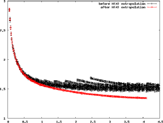
We have analysed the $N_{f}=2+1+1$ ensembles produced by the ETM Collaboration [13], with bare couplings $\beta=2.1$, $1.95$ and $1.9$ that correspond to $a_{\beta=2.1}\sim 0.06$ fm, $a_{\beta=1.95}\sim 0.08$ fm and $a_{\beta=1.9}\sim 0.09$ fm, respectively. Pion masses are in the rang [250-325] MeV. Landau gauge is obtained by standard methods to minimise $A^{\mu}A_{\mu}$ [14] while the ghost propagator is computed by inverting the discretised Faddeev-Popov operator. However, as the O(4) symmetry is broken on the lattice to the H(4) group, getting $\alpha_{T}$ from the dressing functions $G$ and $F$ is not straightforward: ${\cal O}(a^{2}p^{2})$ and H(4) invariants artifacts, the so-called hypercubic artifacts, have to be properly taken into account [15]:

$\displaystyle\alpha_{T}^{\rm Latt}\left(a^{2}p^{2},a^{2}\frac{p^{[4]}}{p^{2}},\dots\right)$ $\displaystyle=$ $\displaystyle\ \widehat{\alpha}_{T}(a^{2}p^{2})$
$\displaystyle+$ $\displaystyle\left.\frac{\partial\alpha_{T}^{\rm Latt}}{\partial\left(a^{2}\frac{p^{[4]}}{p^{2}}\right)}\right|_{a^{2}\frac{p^{[4]}}{p^{2}}=0}\!\!\!\!a^{2}\frac{p^{[4]}}{p^{2}}\ +\ \dots\,,$

$p^{[4]}=\sum_{i}p_{i}^{4}$. We have shown in Fig.ย 3 that a โ€fishboneโ€ structure, that are those hypercubic artifacts, is clearly present in $F$ but curable, as also seen on the plot.

$\hat{\alpha}_{T}(p^{2})$

Refer to caption

Figure 4: Strong coupling constant obtained after the elimination of the dominant hypercubic artifacts

Refer to caption

Figure 5: Raw data of $\alpha_{T}(p^{2})$ compared to a purely perturbative running and OPE with power corrections

Refer to caption

Figure 6: Subtraction of $\alpha_{T}(p^{2})$ from the perturbative running
compared to generic power corrections.

Refer to caption

Figure 7: Comparison of ฮฑsโ€‹(mฯ„)subscript๐›ผ๐‘ subscript๐‘š๐œ\alpha_{s}(m_{\tau}) measured on the lattice with estimates
based on phenomenological analyses of $\tau$ decay data [18], [17].

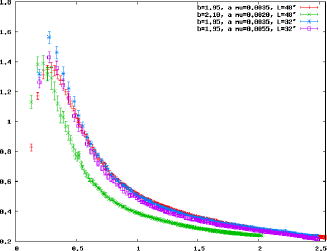
The remaining cut-off effects are removed by fitting $\hat{\alpha}_{T}(p^{2})$ according to the formula $\widehat{\alpha}_{T}(a^{2}p^{2})\ =\ \alpha_{T}(p^{2})\ +\ c_{a2p2}\ a^{2}p^{2}\ +\ {\cal O}(a^{4})$. Fig.ย 4 illustrates the benefit, in term of statistical error on $\alpha_{T}$, to do the calculation in Taylor scheme, as we pointed earlier in the text.
We then use the OPE formalism so that we can relate ฮฑTโ€‹(p2)subscript๐›ผ๐‘‡superscript๐‘2\alpha_{T}(p^{2}) to ฮฑTpertโ€‹(p2)superscriptsubscript๐›ผ๐‘‡pertsuperscript๐‘2\alpha_{T}^{\rm pert}(p^{2}) [16], including power corrections: ฮฑTโ€‹(p2)=ฮฑTpertโ€‹(p2)โ€‹[1+Cโ€‹(p,q0)โ€‹gT2โ€‹(q02)โ€‹โŸจA2โŸฉq02Rp2+dp6+โ‹ฏ]subscript๐›ผ๐‘‡superscript๐‘2subscriptsuperscript๐›ผpert๐‘‡superscript๐‘2delimited-[]1๐ถ๐‘subscript๐‘ž0subscriptsuperscript๐‘”2๐‘‡superscriptsubscript๐‘ž02subscriptsuperscriptdelimited-โŸจโŸฉsuperscript๐ด2๐‘…superscriptsubscript๐‘ž02superscript๐‘2๐‘‘superscript๐‘6โ‹ฏ\alpha_{T}(p^{2})=\alpha^{\rm pert}_{T}(p^{2})\left[1+\frac{C(p,q_{0})g^{2}_{T}(q_{0}^{2})\langle A^{2}\rangle^{R}_{q_{0}^{2}}}{p^{2}}+\frac{d}{p^{6}}+\cdots\right], with q0subscript๐‘ž0q_{0} fixed to 10 GeV and C๐ถC a combination of a Wilson coefficient and a running of the gluonic operator โŸจA2โŸฉdelimited-โŸจโŸฉsuperscript๐ด2\langle A^{2}\rangle. Eventually ฮฑTpertsubscriptsuperscript๐›ผpert๐‘‡\alpha^{\rm pert}_{T} is expressed at N3โ€‹LOsuperscriptN3LO\rm{N^{3}LO} in function of ฮ›Tsubscriptฮ›๐‘‡\Lambda_{T} with ฮ›MSยฏฮ›Tโ‰กexpโก(โˆ’507โˆ’40โ€‹Nf792โˆ’48โ€‹Nf)subscriptฮ›ยฏMSsubscriptฮ›๐‘‡50740subscript๐‘๐‘“79248subscript๐‘๐‘“\frac{\Lambda_{\overline{\rm MS}}}{\Lambda_{T}}\ \equiv\exp\left(\displaystyle-\frac{507-40N_{f}}{792-48N_{f}}\right). The parameters to be fitted are thus aโ€‹ฮ›MSยฏ๐‘Žsubscriptฮ›ยฏMSa\Lambda_{\overline{\rm MS}}, gT2โ€‹โŸจA2โŸฉsubscriptsuperscript๐‘”2๐‘‡delimited-โŸจโŸฉsuperscript๐ด2g^{2}_{T}\langle A^{2}\rangle, d๐‘‘d and the ratios of lattice spacings aฮฒ/a1.9subscript๐‘Ž๐›ฝsubscript๐‘Ž1.9a_{\beta}/a_{1.9} obtained by imposing that the various curves of ฮฑTsubscript๐›ผ๐‘‡\alpha_{T} merge onto a universal one. 
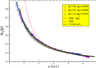
We have shown in Fig.5 that the purely perturbative running formula does not match with the ฮฑTโ€‹(p2)subscript๐›ผ๐‘‡superscript๐‘2\alpha_{T}(p^{2}) data, adding the 1/p21superscript๐‘21/p^{2} fits nicely with them down to p=3.5๐‘3.5p=3.5 GeV while including the 1/p61superscript๐‘61/p^{6} term improves our ability to describe them
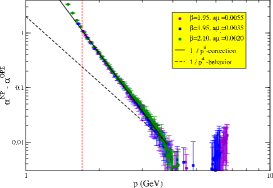
 further down to the ฯ„๐œ\tau mass scale. One could expect a 1/p41superscript๐‘41/p^{4} power correction but Fig.6 indicates that the fit is meaningless: still we do not exclude that the corresponding Wilson coefficient would mimic an additional
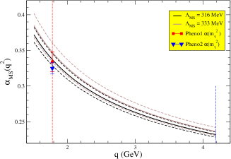
 1/p21superscript๐‘21/p^{2} factor. Collecting in Tab.ย 1 ฮ›MSยฏsubscriptฮ›ยฏMS\Lambda_{\rm\overline{MS}}, g2โ€‹โŸจA2โŸฉsuperscript๐‘”2delimited-โŸจโŸฉsuperscript๐ด2g^{2}\langle A^{2}\rangle and the d๐‘‘d coefficient, with the lattice spacing a1.9=0.08612โ€‹(42)subscript๐‘Ž1.90.0861242a_{1.9}=0.08612(42) fm [13], we can run ฮฑsMSยฏsubscriptsuperscript๐›ผยฏMS๐‘ \alpha^{\overline{\rm MS}}_{s} up to the Z0superscript๐‘0Z^{0} mass scale or at the ฯ„๐œ\tau mass scale. For the latter we obtain ฮฑsMSยฏโ€‹(mฯ„2)=0.337โ€‹(8)subscriptsuperscript๐›ผยฏMS๐‘ subscriptsuperscript๐‘š2๐œ0.3378\alpha^{\rm\overline{MS}}_{s}(m^{2}_{\tau})=0.337(8) and ฮฑsMSยฏโ€‹(mฯ„2)=0.342โ€‹(10)subscriptsuperscript๐›ผยฏMS๐‘ subscriptsuperscript๐‘š2๐œ0.34210\alpha^{\rm\overline{MS}}_{s}(m^{2}_{\tau})=0.342(10) with our 2 estimates of ฮ›MSยฏsubscriptฮ›ยฏMS\Lambda_{\rm\overline{MS}}; combining both of them and adding in quadrature the errors we get ฮฑsMSยฏโ€‹(mฯ„2)=0.339โ€‹(13)subscriptsuperscript๐›ผยฏMS๐‘ subscriptsuperscript๐‘š2๐œ0.33913\alpha^{\rm\overline{MS}}_{s}(m^{2}_{\tau})=0.339(13). It is in very good agreement with ฯ„๐œ\tau decay data analysed with dispersion relations [17], [18], as plotted in Fig.7. Running ฮฑssubscript๐›ผ๐‘ \alpha_{s} up to the MSยฏยฏMS{\rm\overline{MS}} scheme b๐‘b quark mass mbsubscript๐‘š๐‘m_{b}, by using the ฮฒ๐›ฝ\beta function and the ฮ›MSยฏNf=4subscriptsuperscriptฮ›subscriptNf4ยฏMS\Lambda^{\rm N_{f}=4}_{\rm\overline{MS}} parameter we have measured, we can match with the Nf=5subscriptNf5{\rm N_{f}}=5 theory: ฮฑMSยฏNf=5โ€‹(mb2)=ฮฑMSยฏNf=4โ€‹(mb2)โ€‹(1+โˆ‘ncnโ€‹0โ€‹(ฮฑMSยฏNf=4โ€‹(mb))n)subscriptsuperscript๐›ผsubscriptNf5ยฏMSsubscriptsuperscript๐‘š2๐‘subscriptsuperscript๐›ผsubscriptNf4ยฏMSsubscriptsuperscript๐‘š2๐‘1subscript๐‘›subscript๐‘๐‘›0superscriptsubscriptsuperscript๐›ผsubscriptNf4ยฏMSsubscript๐‘š๐‘๐‘›\alpha^{\rm N_{f}=5}_{\rm\overline{MS}}(m^{2}_{b})=\alpha^{\rm N_{f}=4}_{\rm\overline{MS}}(m^{2}_{b})\left(1+\sum_{n}c_{n0}(\alpha^{\rm N_{f}=4}_{\rm\overline{MS}}(m_{b}))^{n}\right). Then a second running is applied up to the Z0superscript๐‘0Z^{0} mass scale. We obtain ฮฑsMSยฏโ€‹(mZ02)=0.1198โ€‹(9)subscriptsuperscript๐›ผยฏMS๐‘ subscriptsuperscript๐‘š2superscript๐‘00.11989\alpha^{\rm\overline{MS}}_{s}(m^{2}_{Z^{0}})=0.1198(9) and ฮฑsMSยฏโ€‹(mZ02)=0.1203โ€‹(11)subscriptsuperscript๐›ผยฏMS๐‘ subscriptsuperscript๐‘š2superscript๐‘00.120311\alpha^{\rm\overline{MS}}_{s}(m^{2}_{Z^{0}})=0.1203(11) with, again, our 2 estimates of ฮ›MSยฏsubscriptฮ›ยฏMS\Lambda_{\rm\overline{MS}}; combining both results and adding in quadrature the errors we get ฮฑsMSยฏโ€‹(mZ02)=0.1200โ€‹(14)subscriptsuperscript๐›ผยฏMS๐‘ subscriptsuperscript๐‘š2superscript๐‘00.120014\alpha^{\rm\overline{MS}}_{s}(m^{2}_{Z^{0}})=0.1200(14). We have shown in Fig.8 a comparison between lattice results [8], [19] and [4], DIS data [20], the world average quoted by the Particle Data Group [21] (WA โ€™12) and a world average realised by replacing the Nf=2+1subscript๐‘๐‘“21N_{f}=2+1 lattice results by the Nf=2+1+1subscript๐‘๐‘“211N_{f}=2+1+1 one (WAโ€™ โ€™12), theoretically more reliable. In [3] one can find an almost exhaustive collection of results. A single, very precise, lattice value dominates strongly the weighted world average of ฮฑsMSยฏโ€‹(mZ02)subscriptsuperscript๐›ผยฏMS๐‘ subscriptsuperscript๐‘š2superscript๐‘0\alpha^{\rm\overline{MS}}_{s}(m^{2}_{Z^{0}}); removing it enlarges its uncertainty. Our estimates is in the same ballpark as other approaches and is using a complementary framework.

Table 1: Fit parameters of $\alpha_{T}(p^{2})$ analysed by means of OPE.
$\Lambda_{\overline{\rm MS}}^{N_{f}=4}$ (MeV) $g^{2}(q_{0}^{2})\langle A^{2}\rangle^{R}_{q^{2}_{0}}$ (GeV2) $d^{1/6}$ (GeV) $\alpha(m_{Z})$
316(13) 4.5(4) 0.1198(9)
324(17) 3.8(1.0) 1.72(3) 0.1203(11)

3 Conclusions

We have reported on the first measurement of ฮฑssubscript๐›ผ๐‘ \alpha_{s} from lattice simulations taking into account the vacuum polarisation effects by charm quark in the so-called ${\rm N_{f}}=2+1+1$ theory. The main benefit of our set-up is that there is no perturbative treatment at the charm threshold. We have used the OPE formalism to analyse gluon and ghost propagators to extract the strong coupling in the MOM Taylor scheme. We have taken care of the hypercubic artifacts and included power corrections in the OPE, that cannot be neglected. An on-going project is to study whether other Green functions (3-gluon vertex, quark propagator,โ€ฆ) present the same feature: our extraction of $\Lambda_{\rm\overline{MS}}$ presented here will help us to reduce the uncertainty on the fits of those Green functions.

K. Petrov acknowledges the support of โ€P2IOโ€ Laboratory of Excellence.

0.1160.1180.120.122ฮฑsโ€‹(mZ)subscript๐›ผ๐‘ subscript๐‘š๐‘\alpha_{s}(m_{Z})${\rm N_{f}}=2+1+1$ ${\rm N_{f}}=2+1$ ${\rm N_{f}}=2+1$DISETMC โ€™12 PACS-CS โ€™11 HPQCD โ€™10 MSTW โ€™08WA โ€™12WAโ€™ โ€™12
Figure 8: Collection of results on ฮฑsโ€‹(mZ)subscript๐›ผ๐‘ subscript๐‘š๐‘\alpha_{s}(m_{Z}).

References

  • [1] ATLAS Collaboration, [arXiv:1207.7214]; CMS Collaboration, [arXiv:1207.7235].
  • [2] J. Baglio and A. Djouadi, JHEP 1103, 055 (2011) [arXiv:1012.0530].
  • [3] S. Bethke et al, [arXiv:1110.0016].
  • [4] B. Blossier et al, Phys. Rev. D 85, 034503 (2012) [arXiv:1110.5829 [hep-lat]]; Phys. Rev. Lett. 108, 262002 (2012) [arXiv:1201.5770].
  • [5] S. Aoki et al, Phys. Rev. D 81, 074503 (2010) [arXiv:0911.2561].
  • [6] S. Dรผrr et al, JHEP 1108, 148 (2011) [arXiv:1011.2711].
  • [7] A. X. El-Khadra et al, Phys. Rev. Lett. 69, 729 (1992).
  • [8] I. Allison et al, Phys. Rev. D 78, 054513 (2008) [arXiv:0805.2999].
  • [9] M. Lรผscher et al, Nucl. Phys. B 389, 247 (1993) [hep-lat/9207010]; Nucl. Phys. B 413, 481 (1994) [hep-lat/9309005].
  • [10] B. Alles et al, Nucl. Phys. B 502, 325 (1997) [hep-lat/9605033]; Ph. Boucaud et al, JHEP 9810, 017 (1998) [hep-lat/9810322]; Phys. Rev. D 63, 114003 (2001) [hep-ph/0101302].
  • [11] A. Sternbeck et al PoS LAT2007, 256 (2007) [arXiv:0710.2965]; Ph. Boucaud et al, Phys. Rev. D 79, 014508 (2009) [arXiv:0811.2059].
  • [12] J. Taylor, Nucl. Phys. B 33, 436 (1971).
  • [13] R. Baron et al, JHEP 1006, 111 (2010) [arXiv:1004.5284]; PoS LATTICE2010, 123 (2010) [arXiv:1101.0518].
  • [14] L. Giusti et al, Int. J. Mod. Phys. A 16, 3487 (2001) [hep-lat/0104012]
  • [15] D. Becirevic et al, Phys. Rev. D 60, 094509 (1999) [hep-ph/9903364]; F. De Soto and C. Roiesnel, JHEP 0709, 007 (2007) [arXiv:0705.3523].
  • [16] B. Blossier et al, Phys. Rev. D 82, 034510 (2010) [arXiv:1005.5290].
  • [17] S. Narison, Phys. Lett. B 673, 30 (2009) [arXiv:0901.3823].
  • [18] A. Pich, [arXiv:1107.1123].
  • [19] S. Aoki et al, JHEP 0910, 053 (2009) [arXiv:0906.3906].
  • [20] A. Martin et al, Eur. Phys. J. C 64, 653 (2009) [arXiv:0905.3531].
  • [21] J. Beringer et al, Phys. Rev. D 86, 010001 (2012).