Calculations of electric fields for radio detection of Ultra-High Energy particles

Abstract

The detection of electromagnetic pulses from high energy showers is used as a means to search for Ultra-High Energy cosmic ray and neutrino interactions. An approximate formula has been obtained to numerically evaluate the radio pulse emitted by a charged particle that instantaneously accelerates, moves at constant speed along a straight track and halts again instantaneously. The approximate solution is applied to the particle track after dividing it in smaller subintervals. The resulting algorithm (often referred to as the ZHS algorithm) is also the basis for most of the simulations of the electric field produced in high energy showers in dense media. In this work, the electromagnetic pulses as predicted with the ZHS algorithm are compared to those obtained with an exact solution of the electric field produced by a charged particle track. The precise conditions that must apply for the algorithm to be valid are discussed and its accuracy is addressed. This comparison is also made for electromagnetic showers in dense media. The ZHS algorithm is shown to describe Cherenkov radiation and to be valid for most situations of interest concerning detectors searching for Ultra-High Energy neutrinos. The results of this work are also relevant for the simulation of pulses emitted from air showers.

I Introduction

The study of Ultra High Energy Cosmic Rays (UHECR) and neutrinos (UHE$\nu$s) is currently a high priority in Astroparticle Physics with many experimental efforts being dedicated to these two related areas of research. UHECRs are routinely detected through the Extensive Atmospheric Showers (EAS) they produce when interacting in the atmosphere. Despite the recent advances in the measurement of the flux of UHECRs  HiRes_spectrum ; Auger_spectrum , their primary composition remains unknown Auger_Xmax ; HiRes_Xmax , and this is one of the main obstacles to extract precise conclusions on their origin. There are strong reasons to believe that UHE$\nu$s should be produced in the interactions of UHECRs with the material surrounding the sources, and/or in their propagation through the observed Cosmic Microwave Background radiation Olinto . However their detection has not yet been achieved. Efforts are being made to improve the experimental situation in both fields. The challenge is to instrument sufficiently large target volumes to compensate for the low cross section and low fluxes for UHE$\nu$ detection, and to find measurements that provide large aperture at the highest energies and help to constrain the primary composition of UHECRs. The radio technique is being explored in both fields.

As early as in 1962, G. Askaryan proposed to detect UHECRs and UHE$\nu$s by observing the coherent radio pulse from the excess of electrons in a shower developing in a dense, dielectric and nonabsorptive to radiowaves medium Askaryan62 . Soon after, pulses were observed in coincidence with air shower arrays Jelley ; Allan . The emission is coherent in wavelengths which are large compared to the characteristic size of the electric charge and current distributions associated to the induced showers. The technique has been receiving a lot of attention in the field of Astroparticle Physics in the last decade because of the relatively low cost of the antennas needed for the detection systems. Also, coherence implies that the pulse energy scales with the square of the primary energy which favours long range detection, a requirement to achieve large areas and volumes both for UHECR and UHE$\nu$ detection. Indeed, quadratic scaling has been confirmed in accelerator experiments  Saltzberg_SLAC_sand ; Miocinovic_SLAC_sand ; Gorham_SLAC_salt ; Gorham_SLAC_ice leading to very strong pulses associated to UHE energy showers.

A large number of initiatives have been made or are currently in development or planning stages. In dense media neutrino-induced showers are less than a meter in width and full coherence is expected to be mantained up to the GHz range (see for instance ZHS92 ). A variety of past and present experiments search for pulses at those frequencies produced by neutrinos in ice RICE03 ; ANITA_2009_limits , the moon regolith Parkes96 ; GLUElimits ; NuMoon ; Kalyazin ; LUNASKA ; RESUN or salt domes Gorham_SLAC_salt . The largest and most promising experiments are in planning stages looking at ice ARA ; ARIANNA . Electromagnetic pulses emitted in the MHz-GHz frequency range by EAS induced by UHECR are being measured in the hope of using this complementary information to constrain its composition and/or to develop new cost effective detection systems AERA ; CODALEMA . In addition the ANITA balloon flown antennas, initially devised to search for neutrinos, has recorded coherent pulses up to the GHz range ANITA_UHECR consistent with EAS induced by UHECRs and there are plans for future developments EVA .

The success of the radio technique requires an accurate and computationally efficient calculation of the radio emission properties of UHE showers. It is necessary to perform this in an efficient way since the number of particles in a shower at EeV energies is $\geq 10^{9}$. Simulation techniques for evaluating pulses in dense media have been used for more than 20 years ZHS91 ; ZHS92 ; alz97 ; alz98 ; alvz99 ; alvz00 ; razzaque01 ; almvz03 ; razzaque04 ; McKay_radio ; alvz06 ; aljpz09 ; ARZ10 ; ZHAireS_ice ; ARZ11 . The shower is simulated to obtain, for every particle track, the information needed to calculate its contribution to the electric field. The formula used for this purpose stems from an approximate solution of Maxwell’s equations in the Fraunhofer limit Allan adapted for simulation purposes in ZHS92 . The electric field due to a short charged particle track, assumed to be travelling at a constant speed, can be approximated by two terms which correspond to the start and end of the track. The resulting electric field depends on the particle speed and the angle between the line of sight from the track to the observer  ZHS92 ; ARZ10 . To calculate the emission in a shower, tracks are chosen so that the particle velocity can be approximated to be constant, and all track contributions are added taking into account interference effects.

Although the approximate formula is sufficient for many practical applications, its range of validity is limited in frequency and position of the observer with respect to the track. It is possible to extend its range of validity by subdividing each track in sub-intervals. The resulting algorithm (often referred to as “ZHS algorithm”) is easy to implement and fast enough for the simulation of particle showers. This is convenient since it has allowed the simulation of pulses in the Fresnel region for neutrino detection alz98 and in measurements of EAS ZHAireS_air . Although the range of applicability of the algorithm is enhanced when used in this way, it is not obvious that the sum of the subcontributions correclty accounts for all the radiation in regions close to the emission source.

The object of this article is to study the conditions for the ZHS algorithm to be valid and to establish its accuracy. For this purpose we obtain in Section II an exact solution to the problem of a charged particle instantaneously accelerating to a constant speed and stopping abruptly after a discrete time interval Tamm . This allows us to establish the precise conditions necessary to turn this solution into the basic formula of the ZHS algorithm. In Section III we compare the exact solutions for an infinite and a finite track to the result of the ZHS algorithm, and stress the compatible interpretation of the radiation regime in terms of Cherenkov radiation for both cases. In Section IV we compare the exact solution of the single track problem in nearby regions with the results of applying the ZHS algorithm with track subdivisions to test its validity and accuracy. Section V is devoted to discussing the ZHS algorithm in relation to other approximations made to calculate the pulses emitted from showers. Section VI presents the summary and conclusions of our work.

II Electromagnetic field of a single charged particle track

Let us assume an electron ejected from an atom at time $t=t_{1}$ that travels at constant speed $\mathbf{v}$ through a medium along a finite track until it is absorbed by another atom at time $t_{2}$. Neglecting the movement of the atoms, we can model the electric current associated to the electron as,

$$\mathbf{J}(\mathbf{x},t)=-e\mathbf{v}\delta^{(3)}(\mathbf{x}-\mathbf{x_{0}}-\mathbf{v}t)~{}\Theta(t-t_{1})\Theta(t_{2}-t)$$ (1)

where $e=|e|$ is the charge of a positron, $\mathbf{x}(t)$ is its position and $\mathbf{x_{0}}$ an arbitrary reference position. The step $\Theta$-functions account for the fact that the electron only moves in the time interval ($t_{1}$, $t_{2}$).

In a dielectric medium with permitivity $\epsilon$ and magnetic susceptibility $\mu$, Maxwell’s equations for the vector potential in the frequency domain $\mathbf{A}(\mathbf{x},\omega)$ can be written as Jackson :

$$\begin{split}&\nabla^{2}\mathbf{A}(\mathbf{x},\omega)+\mu\epsilon\omega^{2}\mathbf{A}(\mathbf{x},\omega)-\\ &\nabla[\nabla\cdot\mathbf{A}(\mathbf{x},\omega)-i\epsilon\mu\omega~{}\phi(\mathbf{x},\omega)]=-\mu\mathbf{J}(\mathbf{x},\omega),\end{split}$$ (2)

where $\phi(\mathbf{x},\omega)$ is the Fourier transform of the scalar potential and we use the following convention for the Fourier-transform of a function $f(t)$: $f(\omega)=\int_{-\infty}^{\infty}\mathrm{d}t\ e^{i\omega t}f(t)$. In principle $\epsilon$ and $\mu$ can depend on frequency and our results below would be equally valid, but we drop the explicit dependence of $\epsilon$ and $\mu$ with $\omega$ for simplicity.

We use the Lorenz gauge condition which implies that Eq. (2) for the vector potential becomes:

$$\nabla^{2}\mathbf{A}+k^{2}\mathbf{A}=-\mu\mathbf{J},$$ (3)

with $k=n\omega/c$ and $n$ the refractive index of the medium. The Lorenz gauge condition in the frequency domain Jackson :

$$\nabla\cdot\mathbf{A}(\mathbf{x},\omega)=i\epsilon\mu\omega~{}\phi(\mathbf{x},\omega),$$ (4)

implies that the scalar potential for non-zero frequencies is entirely determined by the divergence of the vector and only the vector potential is needed to calculate the field.

II.1 Exact solution

The solution of the Helmholtz equation in Eq. (3) is standard physics and can be obtained, using Green’s method, as an integral over source positions Jackson :

$$\mathbf{A}(\mathbf{x},\omega)=\frac{\mu}{4\pi}\int\mathrm{d}^{3}\mathbf{x^{\prime}}\frac{e^{ik|\mathbf{x}-\mathbf{x^{\prime}}|}}{|\mathbf{x}-\mathbf{x^{\prime}}|}\mathbf{J}(\mathbf{x^{\prime}},\omega)$$ (5)

where from now on, $\mathbf{x}$ will denote the position of the observer and $\mathbf{x^{\prime}}$ the position of the source.

For simplicity we rewrite the current in Eq. (1) as:

$$\mathbf{J}(\mathbf{x},t)=qv~{}Z(t)~{}P(\mathbf{x},t)~{}\hat{z}$$ (6)

with $q=-e$; $Z(t)=\Theta(t-t_{1})\Theta(t_{2}-t)$ and $P(\mathbf{x,t})=\delta^{(3)}(\mathbf{x}-vt\hat{z}-z_{0}\hat{z})$, where we assume without loss of generality that the electron travels along the $z$-axis which is parallel to $\hat{z}$. The equations that follow below are clearly valid for any continuous and differentiable functions $Z(t)$ and $P(\mathbf{x},t)$. They are also valid for the case considered in Eq. (1) which can be obtained as a limiting case of suitable continuous and differentiable functions.

Transforming this definition of the current to the frequency domain and substituting into Eq. (5) for the vector potential we obtain:

$$\mathbf{A}(\mathbf{x},\omega)=\frac{\mu}{4\pi}~{}qv~{}\hat{z}~{}\int\mathrm{d}^{3}\mathbf{x^{\prime}}\mathrm{d}t^{\prime}~{}e^{i\omega t^{\prime}}\frac{e^{ik|\mathbf{x}-\mathbf{x^{\prime}}|}}{|\mathbf{x}-\mathbf{x^{\prime}}|}Z(t^{\prime})P(\mathbf{x^{\prime}},t^{\prime})$$ (7)

In the Lorenz gauge, the only non-zero component of the vector potential for a charge moving along $z$ is the $z$-component. The scalar potential $\phi$ is obtained through Eq. (4). For this purpose we need to obtain $\nabla\cdot\mathbf{A}$:

$$\nabla\cdot\mathbf{A}(\mathbf{x},\omega)=\frac{\partial A_{z}}{\partial z}=\frac{\mu}{4\pi}~{}qv~{}\int\mathrm{d}^{3}\mathbf{x^{\prime}}\mathrm{d}t^{\prime}~{}Z(t^{\prime})P(\mathbf{x^{\prime}},t^{\prime})$$

$$e^{i\omega t^{\prime}}~{}\frac{e^{ik|\mathbf{x}-\mathbf{x^{\prime}}|}}{|\mathbf{x}-\mathbf{x^{\prime}}|}\left[ik-\frac{1}{|\mathbf{x}-\mathbf{x^{\prime}}|}\right]\frac{(z-z^{\prime})}{|\mathbf{x}-\mathbf{x^{\prime}}|}$$

The electric field $\mathbf{E}(\mathbf{x},\omega)$ can be obtained from the scalar and vector potentials Jackson as:

$$\mathbf{E}(\mathbf{x},\omega)=-\nabla\phi(\mathbf{x},\omega)+i\omega\mathbf{A}(\mathbf{x},\omega)$$ (8)

Due to the cylindrical symmetry of a charged particle track we calculate only the radial ($E_{\rho}$) and $z$ ($E_{z}$) components of the field. Since $\mathbf{A}$ only has $z$-component, then the radial component of the field is given by:

$$E_{\rho}(\mathbf{x},\omega)=-\frac{\partial\phi(\mathbf{x},\omega)}{\partial\rho}=-\partial_{\rho}\frac{\nabla\cdot\mathbf{A}(\mathbf{x},\omega)}{i\mu\epsilon\omega}$$ (9)

where $\rho=\sqrt{x^{2}+y^{2}}$ is the radial coordinate, and $\partial_{\rho}$ denotes $\partial/\partial\rho$.

The $z-$component of the field is given by:

$$E_{z}(\mathbf{x},\omega)=-\partial_{z}\phi(\mathbf{x},\omega)+i\omega A_{z}(\mathbf{x},\omega)$$

$$=-\partial_{z}\frac{\nabla\cdot\mathbf{A}(\mathbf{x},\omega)}{i\omega\mu\epsilon}+i\omega A_{z}(\mathbf{x},\omega)$$ (10)

with $\partial_{z}$ denoting $\partial/\partial z$.

Performing the derivatives in Eqs. (9) and (10) we obtain:

$$\begin{split}&E_{\rho}(\mathbf{x},\omega)=i~{}\frac{qv}{\omega}~{}\frac{1}{4\pi\epsilon}\int_{t_{1}}^{t_{2}}\mathrm{d}t^{\prime}~{}e^{i\omega t^{\prime}}~{}\frac{e^{ikr}}{r^{3}}\times\\ &\rho\times(z-z_{0}-vt^{\prime})\times\left[b\left(b-\frac{1}{r}\right)+\frac{1}{r^{2}}\right]\end{split}$$ (11)

and,

$$\begin{split}&E_{z}(\mathbf{x},\omega)=i~{}\frac{qv}{\omega}~{}\frac{1}{4\pi\epsilon}~{}\int_{t_{1}}^{t_{2}}\mathrm{d}t^{\prime}~{}e^{i\omega t^{\prime}}\frac{e^{ikr}}{r^{2}}~{}\times\\ &\Bigg{[}b^{2}\frac{(z-z_{0}-vt^{\prime})^{2}}{r}~{}+~{}\frac{(z-z_{0}-vt^{\prime})^{2}}{r^{3}}~{}-~{}\\ &b\left(\frac{(z-z_{0}-vt^{\prime})^{2}}{r^{2}}-1\right)\Bigg{]}~{}+~{}\\ &i\omega~{}\frac{\mu}{4\pi}~{}qv~{}\int_{t_{1}}^{t_{2}}\mathrm{d}t^{\prime}~{}e^{i\omega t^{\prime}}~{}\frac{e^{ikr}}{r}\end{split}$$ (12)

where $r=r(t^{\prime})$ and $b=b(t^{\prime})$ are both functions of the source time $t^{\prime}$ which is defined as,

$$r(t^{\prime})=|\mathbf{x}-\mathbf{x^{\prime}}|=\sqrt{\rho^{2}+(z-z_{0}-vt^{\prime})^{2}}$$ (13)

and

$$b(t^{\prime})=ik-\frac{1}{r(t^{\prime})}$$ (14)

Eqs. (11) and (12) provide an exact solution for the electric field of a finite track. In general they do not have an analytical form and a numerical integration needs to be performed to obtain the field. For the calculations in this paper, we have divided the integration interval and applied Simpson’s rule, increasing the number of divisions until the integral converged. Under certain conditions, however, we can give analytical approximations for relevant physical situations.

In the following we show that the basic expression used in the ZHS algorithm is a particular case of Eqs. (11) and (12) under certain approximations.

II.2 The ZHS expression

A simple expression for the approximate calculation of the electric field from a single charged particle track moving at constant speed was found in ZHS92 . In this section we derive the expression used for the ZHS algorithm from the exact solution and compare the electric field as obtained in both the exact calculation and with the ZHS expression. This allows us to establish under which circumstances the formula gives a good account of the electric field.

The ZHS algorithm can be obtained from Eqs. (11) and (12) if the following set of conditions are fulfilled:

1. The observer is in the “far field” zone i.e.

   $$kr\gg 1$$ (15)

2. The Fraunhofer approximation holds. This can be stated as a condition for the phase factor to be approximated as:

   $$kr=k|\mathbf{x}-\mathbf{x^{\prime}}|\approx k[R-v(t-t_{0})\cos\theta]$$ (16)

   where $R$ is the distance from the observation point to a reference point along the track where the particle is located at a reference time $t_{0}$, and $\theta$ is the angle between the particle track and the direction from the reference point to the observer. This approximation holds provided the parameter $\eta\ll 1$ with $\eta$ defined as:

   $$\eta(t)=\frac{k[v(t-t_{\rm 0})]^{2}}{R}\sin^{2}\theta,$$ (17)

   This condition should be fulfilled at any time $t$ from $t_{1}$ to $t_{2}$. A more commonly used and nearly equivalent form of this condition buniy02 is:

   $$\eta^{\prime}=\frac{kL^{2}}{R}\sin^{2}\theta\ll 1,$$ (18)

   where $L=v(t_{2}-t_{1})$ is the length of the track. This condition is necessary to ensure that the second and higher order terms for the phases $i(\omega t+kr)$ in Eqs. (11) and (12) have no relevance, even when the sum of the leading and first order terms in the Taylor expansion of the phases is zero, as it occurs for observation at the Cherenkov angle Afanasiev_book defined as $\cos\theta_{C}=1/\beta n$ with $\beta=v/c$.

3. Finally the distance to the observer appearing in the denominators of several terms of Eqs. (11) and (12) must be approximated as:

   $$\frac{1}{r(t)}\approx\frac{1}{R}$$ (19)

   over the length $L$ of the track, where $R$ is the distance to a reference point along the track (in the ZHS algorithm the mid-point of the track is selected). The error when making this approximation is of order $L/R$.

In particular, the condition in Eq. (15) implies:

$$b(t^{\prime})\approx ik~{};\qquad b-\frac{1}{r}\approx b~{};\qquad b^{2}+\frac{1}{r^{2}}\approx b^{2}$$ (20)

With these approximations the radial component of the field in Eq. (11) becomes:

$$\begin{split}&E_{\rho}\approx i\frac{qv}{\omega}~{}\frac{1}{4\pi\epsilon}~{}\frac{e^{ikR}}{R}~{}(ik)^{2}~{}\sin\theta\cos\theta~{}e^{i\mathbf{k}\cdot\mathbf{v}t_{0}}~{}\\ &\int_{t_{1}}^{t_{2}}\mathrm{d}t^{\prime}~{}e^{i(\omega-\mathbf{k}\cdot\mathbf{v})t^{\prime}}\end{split}$$ (21)

where we have used:

$$\frac{\rho}{r}\approx\frac{\rho}{R}=\sin\theta,$$ (22)

and

$$\frac{z-z_{0}-vt}{r}\approx\frac{z-z_{0}-vt_{0}}{R}=\cos\theta.$$ (23)

Eq. (21) can be easily integrated yielding:

$$\begin{split}&E_{\rho}=-iq~{}\omega~{}\frac{\mu}{4\pi}~{}v\sin\theta\cos\theta~{}\frac{e^{ikR}}{R}~{}\\ &e^{i\mathbf{k}\cdot\mathbf{v}t_{0}}~{}\left[\frac{e^{i(\omega-\mathbf{k}\cdot\mathbf{v})t_{2}}-e^{i(\omega-\mathbf{k}\cdot\mathbf{v})t_{1}}}{i(\omega-\mathbf{k}\cdot\mathbf{v})}\right].\end{split}$$ (24)

If we make $t_{0}=t_{1}$ this becomes the expression for the radial field as used in the ZHS algorithm ZHS92 except for a factor 2 due to the Fourier transform convention used in ZHS92 .

Similarly applying the approximations in Eqs. (16), (19) and (20) to Eq. (12) for the $z$-component of the field, and using that $kR\gg 1\Rightarrow k^{2}\gg k/R$, it is straightforward to show that:

$$\begin{split}&E_{z}\approx-i\omega^{2}~{}\frac{qv}{\omega}\frac{\mu}{4\pi}~{}\frac{e^{ikR}}{R}~{}e^{i\mathbf{k}\cdot\mathbf{v}~{}t_{0}}\cos^{2}\theta~{}\int_{t_{1}}^{t_{2}}\mathrm{d}t\ e^{i(\omega-\mathbf{k}\cdot\mathbf{v})t}\\ &+iqv~{}\omega~{}\frac{\mu}{4\pi}~{}\frac{e^{ikR}}{R}~{}e^{i\mathbf{k}\cdot\mathbf{v}t_{0}}~{}\int_{t_{1}}^{t_{2}}\mathrm{d}t\ e^{i(\omega-\mathbf{k}\cdot\mathbf{v})t}~{},\end{split}$$ (25)

which can be cast as:

$$E_{z}=iq~{}\omega~{}\frac{\mu}{4\pi}~{}v\sin^{2}\theta~{}\frac{e^{ikR}}{R}~{}e^{i\mathbf{k}\cdot\mathbf{v}t_{0}}\int_{t_{1}}^{t_{2}}\mathrm{d}t\ e^{i(\omega-\mathbf{k}\cdot\mathbf{v})t}$$ (26)

Performing the integral, and taking $t_{0}=t_{1}$, the ZHS formula is recovered:

$$\begin{split}&E_{z}=iq~{}\omega\frac{\mu}{4\pi}~{}v\sin^{2}\theta~{}\frac{e^{ikR}}{R}~{}\\ &e^{i\mathbf{k}\cdot\mathbf{v}t_{1}}~{}\left[\frac{e^{i(\omega-\mathbf{k}\cdot\mathbf{v})t_{2}}~{}-e^{i(\omega-\mathbf{k}\cdot\mathbf{v})t_{1}}}{i(\omega-\mathbf{k}\cdot\mathbf{v})}\right]~{}.\end{split}$$ (27)

II.3 The ZHS algorithm

To calculate the electric field of the pulse emitted from a current distribution, such as that produced in a high energy shower, the ZHS algorithm uses the ZHS expressions in Eqs. (24) and (27) to calculate the emission from all the charged particle tracks. The final result is obtained adding up all the contributions. The value of $R$ used for the phase factor in each particle track is the distance from the first point of the track to the observation point. This definition is consistent with the convention to account for the phase change between emission arising from the start and end points of the track. The actual value of $R$ used for the denominator is the distance between the midpoint of the track and the observer which is for all practical purposes the same value when the approximation is valid. The algorithm used in alternative simulation programs is similar but different in these technical details endpoints .

Naturally it is possible to divide any charged particle track into arbitrarily small subtracks in order to make the computation more accurate. This will extend the range of validity of the approximation. It is interesting to note that it makes absolutely no difference to subdivide the track of a uniformly moving charge when observed in the Fraunhofer limit because the term associated to the end of one subtrack cancels the term associated to the beginning of the next subtrack. This is because in this limit the differences in $R$ between adjacent subtracks are arbitrarily small. However in practical situations this cancelation is not exact if $R$ is allowed to change from a track to the next one according to geometry. In the original ZHS program ZHS91 the tracks were not subdivided but soon it was realized that a more accurate result was obtained by subdividing all tracks at every point there was a discrete interaction in the simulation program ZHS95 ; alvz00 . This was the main modification that was ever made to the original ZHS Monte Carlo ZHS91 ; ZHS92 and has been effective since then. With this subdivision the distribution of tracks for a shower in ice has a peak at about $L\sim 1~{}$mm.

III Cherenkov radiation

The exact electric field for a charged particle track derived in Eqs. (11) and (12) must account for every single feature of the electric field, since no approximations have been made. In particular, it must reproduce Cherenkov radiation which is the only radiation emitted by a charged particle moving at constant speed, when $v>c/n$ in the limit of an infinite track. An analytical solution for the electric field produced by such particle can be obtained and it is given in Afanasiev_book (chapter 4). The radial $\rho$ and $z-$components of the fields given in Afanasiev_book converted to SI units, and using the Fourier transform convention adopted in this work, can be written as:

$$E_{\rho}(\rho,z,\omega)=\frac{q}{2\pi\epsilon v}e^{i\frac{\omega}{v}z}uK_{1}(u\rho)$$ (28)

$$E_{z}(\rho,z,\omega)=\frac{i\omega\mu q}{2\pi}e^{i\frac{\omega}{v}z}\left(1-\frac{1}{\mu\epsilon v^{2}}\right)K_{0}(u\rho)~{},$$ (29)

where $\rho$ is the radial coordinate, $K_{0}$ and $K_{1}$ are the modified Bessel functions of the second kind, and $u=u(\omega)$ is a function that can take two different values depending on the magnitude of the particle speed, $v<c/n$ or $v>c/n$ (subluminal or superluminal regime). In our convention:

$$v<\frac{c}{n}\Rightarrow u(\omega)=\frac{\omega}{v}\left|\sqrt{1-n^{2}\beta^{2}}\right|$$ (30)

$$v>\frac{c}{n}\Rightarrow u(\omega)=-i\frac{\omega}{v}\left|\sqrt{n^{2}\beta^{2}-1}\right|.$$ (31)

If the particle travels below the speed of light in the medium, the argument $u(\omega)$ of the Bessel functions is real and the particle does not radiate as shown in Afanasiev_book . On the contrary, if the speed of the particle is larger than the speed of light, then $u(\omega)$ is imaginary and the particle radiates. The latter case corresponds to pure Cherenkov radiation Afanasiev_book .

With the help of the asymptotic forms for the Bessel functions, we can obtain the limits of Eqs. (28) and (29) when $|u\rho|\ll 1$ i.e. for small distances to the track compared to the radiation wavelength. Conversely we can also obtain the limits when $|u\rho|\gg 1$ i.e. for large distances compared to the wavelength. If $|u\rho|\ll 1$ the $K_{1}$ Bessel function dominates over the $K_{0}$ and only the radial component of the field $E_{\rho}$ matters. In this case,

$$\lim_{|u\rho|\rightarrow 0}|E_{\rho}|=\frac{|q|}{2\pi\epsilon v}\frac{1}{\rho}$$ (32)

and a $1/\rho$ dependence with distances is obtained, as well as no dependence with frequency.

If $|u\rho|\gg 1$ and keeping in mind that when $v>c/n$ the argument $u$ is imaginary the fields can be written as:

$$\lim_{u\rho\rightarrow\pm i\infty}|E_{\rho}|=\frac{|q|}{2\pi\epsilon v}\sqrt{\frac{\pi}{2}}\left|(n^{2}\beta^{2}-1)^{1/4}\sqrt{\frac{\omega}{v\rho}}\right|$$ (33)

$$\lim_{u\rho\rightarrow\pm i\infty}|E_{z}|=\frac{\mu|q|}{2\pi}\left(1-\frac{1}{\mu\epsilon v^{2}}\right)\sqrt{\frac{\pi}{2}}$$

$$\left|\frac{1}{(n^{2}\beta^{2}-1)^{1/4}}\sqrt{\frac{v\omega}{\rho}}\right|$$ (34)

In this case the field is proportional to $\sqrt{\omega/\rho}$. This is in agreement with buniy02 where the same behavior is deduced using simple arguments of energy conservation through a cylindrical surface surrounding the track.

In Fig. 1 the Fourier components of the modulus of the electric field for an infinite track as obtained from Eqs. (28) and (29) are shown, for different frequencies, as a function of $\rho$, the radial distance to the track. The particle speed is $v\simeq c>c/n$ travelling in homogeneous ice with refractive index $n=1.78$. Under these circumstances the quantity $|u\rho|$ can be approximated as:

$$|u\rho|\approx 3\left(\frac{\nu}{100~{}{\rm MHz}}\right)~{}\left(\frac{\rho}{1~{}{\rm m}}\right)$$ (35)

At large distances to the track when $|u\rho|\gg 1$ the fields shown in Fig. 1 scale with distance as $1/\sqrt{\rho}$ and with frequency as $\sqrt{\omega}$, in agreement with the aysmptotic field components in Eqs. (33) and (III). This behavior takes place when $\rho>0.1$, 1 and 10 m for frequencies $\nu=1$ GHz, 100 MHz and 10 MHz respectively, in agreement with Eq. (35), as can be seen in Fig. 1.

As the distance to the track decreases and the condition $|u\rho|\ll 1$ starts to be valid, the field behaves as $1/\rho$ and does not depend on frequency as expected from Eq. (32). As can be clearly seen in Fig. 1, the transition from the $1/\rho$ behaviour to $\sqrt{\omega/\rho}$ occurs at a distance that depends on frequency because $|u\rho|$ involves the frequency (Eq. 35). For instance at distances $\rho<0.01$ m the condition $|u\rho|\ll 1$ applies for both $\nu=100$ and 10 MHz. The Fourier component of the field scales with $1/\rho$ and has the same value for the two frequencies as seen in Fig. 1, while this is not the case for a frequency of $\nu=1$ GHz.

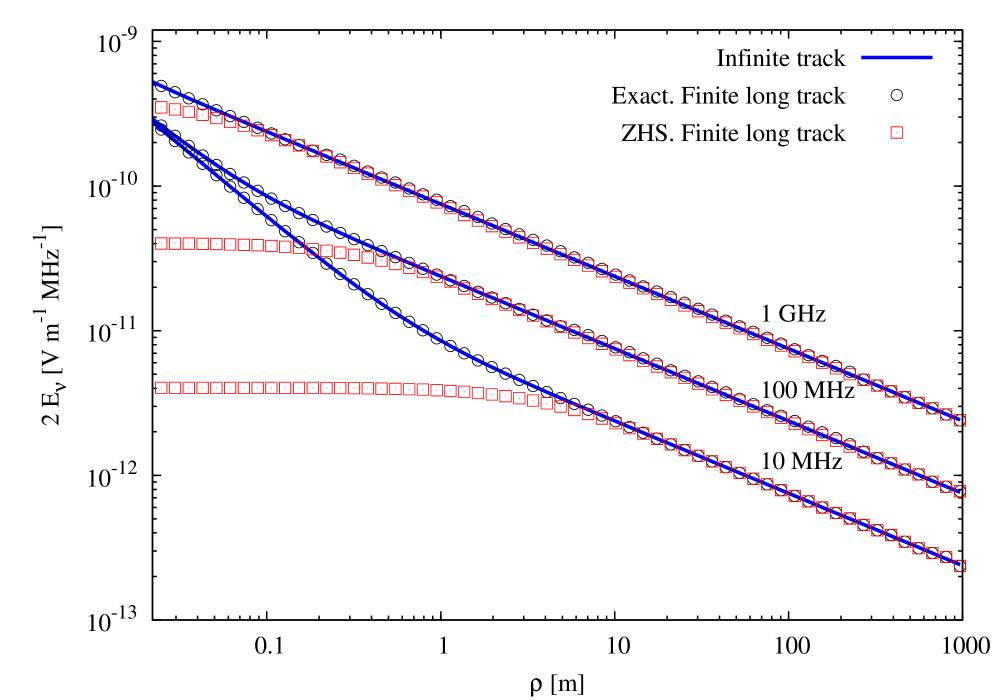
Figure 1: Fourier components of the electric field modulus as a function of distance to the particle track for an infinite track as obtained from Eqs. (28) and (29) (solid line), and for a track of length $L=1200$ m as obtained with the exact formulas derived in this work (Eqs. (11) and (12)) (open circles) and with the ZHS algorithm (Eqs. (24) and (27)) (open squares). From top to bottom, the observation frequencies are $1$ GHz, $100$ MHz and $10$ MHz. The $1/\rho$ and $1/\sqrt{\rho}$ regimes are apparent.

In Fig. 2 the modulus of the field for a charged particle in an infinite track - as obtained from Eqs. (28) and (29) - is shown as a function of frequency for an observer at a fixed radial distance. At large enough frequencies so that the condition $|u\rho|\gg 1$ applies, the field scales as $\sqrt{\omega}$ as expected from Eqs. (33) and (III), while it is constant with frequency for small enough frequencies so that $|u\rho|\ll 1$ as predicted from the asymptotic Eq. (32). More quantitatively, since the observer in Fig. 2 is located at $\rho\sim 10$ m, the field should behave as $\sqrt{\omega}$ for $\nu\lower 3.01385pt\hbox{$\;\stackrel{{\scriptstyle\textstyle>}}{{\sim}}\;$}10$ MHz (applying Eq. (35)). This is approximately the case as can be seen in Fig. 2.

The result of the exact calculation for a track of length $L=1.2$ km is also shown in Figs. 1 and 2. The agreement between both calculations is excellent because the finite track is long compared to observation distance. This confirms that Eqs. (11) and (12) must also account for Cherenkov radiation. As can be appreciated in Fig. 2, the exact results for finite and infinite tracks differ for wavelengths larger than the length of the track - frequencies typically below $\nu_{0}\sim(c/n)/\lambda$ with $\lambda\sim L=1.2$ which gives $\nu\lower 3.01385pt\hbox{$\;\stackrel{{\scriptstyle\textstyle<}}{{\sim}}\;$}0.1$ MHz.

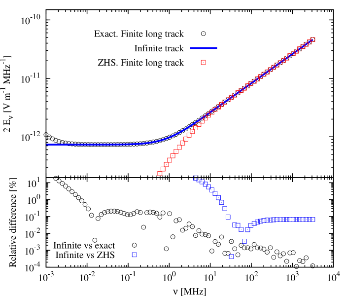
Figure 2: Top panel: Fourier components of the electric field modulus as a function of frequency for an infinite track as obtained from Eqs. (28) and (29) (solid line), and for a track of length $L=1200$ m as calculated in this work from Eqs. (11) and (12) (open circles). The observer is placed at a lateral distance to the infinite track $\rho=8.27$ m. Also shown is the modulus of the field for the same finite track ($L=1.2$ km) as obtained with the ZHS algorithm, Eqs. (24) and (27) (open squares). At high frequencies, the field behaves with $\sqrt{\omega}$ (see text for explanations). Bottom panel: Relative difference (in $\%$) between the solution for an infinite track and the exact solution for a finite long track (open circles) and between the solution for an infinite track and that obtained with the ZHS algorithm (open squares).

IV Comparison of the exact calculation and the ZHS algorithm

We have numerically evaluated the exact expressions for the $z$ and $\rho$ components of the electric field in Eqs. (11) and (12) at different frequencies and observer distances, for a single tracks of different lenghts, and for the tracks constituting a shower in ice as obtained in full simulations performed with the ZHS Monte Carlo code ZHS92 . In this section we present the results of this comparison.

IV.1 Fourier components of the electric field for a single track

The applicability of the ZHS expressions in Eqs. (24) and (27) relies on the conditions $1-3$ in Section II.2. Eqs. (17) and (19) are easily fulfilled for any wavenumber $k$ simply by dividing the particle track in a sufficiently large number of subtracks. Once this is guaranteed, the ZHS expression is applied to every sub-track and the electric field is obtained adding the corresponding contributions. The validity of this procedure will be numerically confirmed below when comparing the exact calculation with the electric field obtained using the ZHS algorithm in the manner just described. However the condition $kr\gg 1$, Eq. (15), does not depend on the size of the track and cannot be enforced by applying the procedure outlined above. As a consequence $kr\gg 1$ is an intrinsic limit to the range of observing frequencies and distances in which the ZHS algorithm gives accurate results as will be shown in the following.

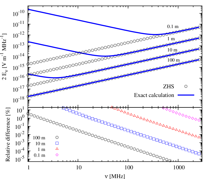
Figure 3: Top panel: Fourier components of the electric field modulus for a single particle track as obtained with the exact calculation Eqs. (11) and (12) (solid lines) and with the ZHS algorithm Eqs. (24) and (27) (open symbols). The length of the track is $L=1.2~{}10^{-3}$ m and the field is shown for observers at distances (from top to bottom lines) $R=0.1$ m, 1 m, 10 m and 100 m, with respect to the center of the track, and placed at the Cherenkov angle. Bottom panel: Relative difference (in $\%$) between the exact solution and that obtained with the ZHS algorithm for the same distances.

In Fig. 3 we compare the Fourier components of the electric field modulus for a single particle track as obtained with the exact calculation, Eqs. (11) and (12), to that obtained with the ZHS algorithm. The length of the track is chosen to be small $L=1.2~{}10^{-3}$m (close to the peak value of the distribution of track lengths in the standard ZHS code). To test the validity of the ZHS algorithm, we have calculated the spectra for observers at different distances ($R$) measured with respect to the center of the track and placed at the Cherenkov angle.

The condition $kR\gg 1$ in ice with refractive index $n=1.78$ can be cast as:

$$kR\sim 3.7~{}\left(\frac{\nu}{100~{}{\rm MHz}}\right)~{}\left(\frac{R}{1~{}{\rm m}}\right)\gg 1$$ (36)

For observers at distances $R=100,~{}10,~{}1$ and $0.1$ m from the particle track, the condition in Eq. (36) is fulfilled as long as $\nu\lower 3.01385pt\hbox{$\;\stackrel{{\scriptstyle\textstyle>}}{{\sim}}\;$}1,10,100$ MHz and 1 GHz respectively. The ZHS algorithm is expected to reproduce the results of the exact calculation in this range. This can be seen in Fig. 3. The relative difference between the ZHS and exact calculations is less than $\sim 2\%$ at the frontier of the validity range in the explored frequency and distance space. The accuracy can be however orders of magnitude better. If $kR>37$ is enforced for instance the corresponding relative difference is below $\sim 0.01\%$. This condition is satisfied for $R>10$ m and $\nu\lower 3.01385pt\hbox{$\;\stackrel{{\scriptstyle\textstyle>}}{{\sim}}\;$}100$ MHz what corresponds to a range of frequencies and distances typically encountered in experiments that search for neutrino induced radio transients.

What is striking is that these conclusions also apply in the “near field” provided the track is subdivided in sufficiently small sub-tracks. This can be seen in Fig. 4 comparing the exact and ZHS results for a $L=1.2$ m track. The same range of validity is obtained because conditions (16), (17) and (19) are guaranteed by reducing the length of the sub-tracks.

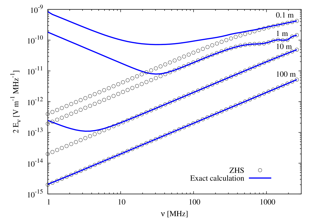
Figure 4: Same as top panel of Fig. 3 for a single particle track of length $L=1.2$ m.

For fixed frequencies the condition in Eq. (36) only applies at sufficiently large distances $R$ to the track. This is illustrated in Fig. 5 for a track of length $L=1.2$ m. The Fourier components at frequencies of $\nu=10$, 100 MHz and 1 GHz are in agreement with the exact calculation respectively at $R\lower 3.01385pt\hbox{$\;\stackrel{{\scriptstyle\textstyle>}}{{\sim}}\;$}10$, 1 and 0.1 m as expected. Since the typical distance between antennas in experiments such as the Askaryan Radio Array (ARA) ARA is $\sim 10-100$ m, we expect the results of the ZHS algorithm obtained through the procedure outlined above, to be accurate enough in most practical situations.

It has been questioned whether the ZHS algorithm reproduces Cherenkov radiation from a single charged particle track endpoints . In Figs. 1 and 2 the algorithm is shown to be in very good agreement with the exact solution for a 1.2 km track as long as $kR\gg 1$ as explained above. The emission from such track is in turn practically equivalent to the Cherenkov emission from an infinite track (also displayed) and it follows that the ZHS calculation must account for Cherenkov radiation.

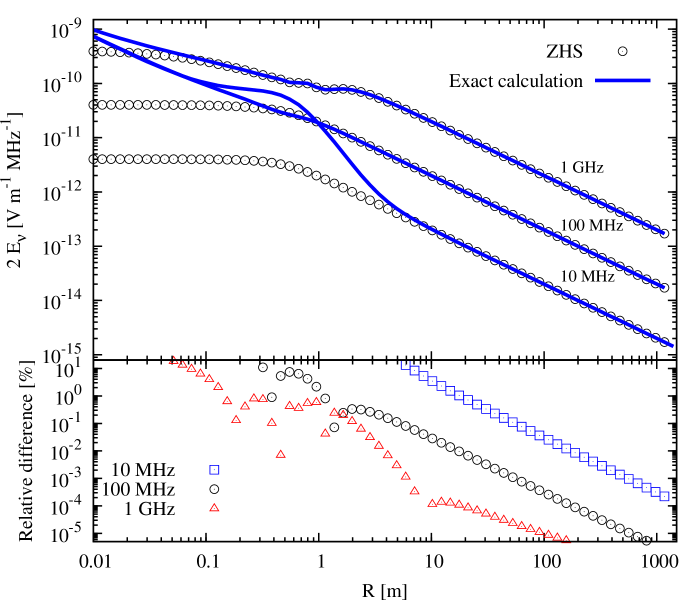
Figure 5: Top panel: Fourier components of the electric field modulus at $\nu=1$ GHz, 100 MHz and 10 MHz (from top to bottom lines) for a single particle track as a function of distance to the track, as obtained with the exact calculation Eqs. (11) and (12) (solid lines) and with the ZHS algorithm Eqs. (24) and (27) (open symbols). The length of the track is $L=1.2$ m and the observers are placed at the Cherenkov angle. Bottom panel: Relative difference (in $\%$) between the exact solution and that obtained with the ZHS algorithm for the same frequencies.

IV.1.1 Behaviour of the field with frequency

As can be seen in Fig. 3 (solid lines) the exact solution for the modulus of the electric field scales linearly with frequency provided that $kR\gg 1$. As a result the electric field can be approximated with the ZHS expressions, Eqs. (24) and (27). For an observer close to the Cherenkov angle as in Fig. 3, the factor $(\omega-\mathbf{k}\cdot\mathbf{v})\ll 1$ and the term in brackets in Eqs. (24) and (27) can be approximated by:

$$\begin{split}&~{}\left[\frac{e^{i(\omega-\mathbf{k}\cdot\mathbf{v})t_{2}}~{}-e^{i(\omega-\mathbf{k}\cdot\mathbf{v})t_{1}}}{i(\omega-\mathbf{k}\cdot\mathbf{v})}\right]\approx\\ &\frac{1+i(\omega-\mathbf{k}\cdot\mathbf{v})t_{2}-1-i(\omega-\mathbf{k}\cdot\mathbf{v})t_{1}}{i(\omega-\mathbf{k}\cdot\mathbf{v})}=t_{2}-t_{1}\end{split}$$ (37)

making the dependence of the field with $\omega$ apparent. Clearly the field cannot grow indefinetely with frequency. This apparent “ultraviolet divergence” is only an artifact of considering the unrealistic medium in which the permittivity $\epsilon(\omega)$ is constant with frequency. In a physical medium absorption at high frequencies will tame the growth with frequency of the electric field.

When $kR<1$ the field behaves with frequency as $\omega^{-1}$ as can be also seen in Fig. 3. In the model of a charged particle at rest for $t\leq t_{1}$, moving with a speed $v$ between $t=t_{1}$ and $t=t_{2}$, and becoming again at rest for $t\geq t_{2}$, the Coulomb field dominates at small distances to the track and/or low frequencies. The field can be modeled as:

$$E_{1}\propto\frac{1}{r_{1}^{2}}~{}\Theta(t_{1,obs}-t)$$ (38)

for $t<t_{1}$ and

$$E_{2}\propto\frac{1}{r_{2}^{2}}~{}\Theta(t-t_{2,obs})$$ (39)

for $t>t_{2}$, where $r_{1}$ and $r_{2}$ are respectively the distances from the charge to the observer at times $t_{1}$ and $t_{2}$, and $t_{1,obs}$ and $t_{2,obs}$ denote the instants of time at which the Coulomb field arrives at the observer. The Fourier transform of a Heaviside function at non-zero frequency is proportional to $\omega^{-1}$, and the two Coulomb fields interfere coherently at low frequencies, explaining the frequency dependence of the electric field. Naturally the ZHS algorithm does not reproduce this behavior which is not associated to radiation. The growth of the field at low frequencies is an artifact of not accounting for screening of the field by the atoms in the medium.

IV.1.2 Behavior of the field with distance

In Fig. 5 the dependence of the Fourier components of the field modulus with distance is shown for several frequencies. At sufficiently large distances to the track the electric field behaves as $1/R$ for all frequencies. This is the radiation zone, the field is expected to behave as $1/R$ as explained in conventional radiation theory Jackson . If the observer is placed at very small distances compared to the length of the track, the situation resembles that of an infinite track. In this case the discussion in Section III applies. The field behaves as $1/\sqrt{R}$ at distances much smaller than the length of the track provided the frequency is high enough to satisfy $|u\rho|\gg 1$ - see Eq. (35). This can be seen in the curve of the Fourier component at $\nu=1$ GHz for $R\lower 3.01385pt\hbox{$\;\stackrel{{\scriptstyle\textstyle<}}{{\sim}}\;$}0.5$ m. At small distances and sufficiently low frequencies, when $|u\rho|\ll 1$, the field becomes proportional to $1/R$ and independent of frequency - see Eq. (29). This feature can be appreciated in Fig. 5 at distances below 0.1 m for the calculations at 10 and 100 MHz. The ZHS algorithm reproduces the calculation provided the $kR\gg 1$ condition is satisfied as could be expected, reproducing both the $1/R$ and $1/\sqrt{R}$ behaviors.

IV.2 Fourier components of the electric field in electromagnetic showers

It is possible to test the ZHS algorithm in a more realistic situation. In this section we compare the Fourier components of the electric field predicted by the ZHS algorithm with those obtained using the exact calculation in a full simulation of electromagnetic showers.

For this purpose we have applied the exact solutions of the field of a track given in Eqs. (11) and (12) in the ZHS Monte Carlo code ZHS92 for the simulation of electron and photon-induced showers in ice. The ZHS Monte Carlo calculates the start and end points of small sub-tracks of all charged particles (electrons and positrons) in an electromagnetic shower down to a kinetic energy threshold of $\sim 100$ keV. With these we can calculate the exact electric field produced by each single sub-track and add the fields up accounting for interference between different tracks. Since Eqs. (11) and (12) are only valid for a charged particle travelling along the $z$ axis (parallel to the shower axis), we perform the necessary rotations of Eqs. (11) and (12) to obtain the field for a particle track moving along an arbitrary direction.

Simultaneously with the exact calculation, we also obtain the field as predicted by the ZHS algorithm for exactly the same shower (i.e. the same set of tracks and sub-tracks). As explained above the subdivisions are such that the conditions in Eqs. (16), (17) and (19) are fulfilled for all the sub-tracks in the shower.

The result is qualitatively the same as in the case of single tracks. As long as the condition $kR\gg 1$ is fulfilled, the ZHS algorithm gives an accurate prediction for the Fourier components of the electric field with a difference of less than a few percent relative to those obtained with the exact calculation. As can be seen in Fig. 6 this occurs for distances to the shower axis as small as $R=1$ m and frequencies above $\nu\sim 10$ MHz, well in the distance and frequency ranges relevant for experiments looking for particle shower induced radio pulses in dense media ARA ; ARIANNA ; RICE03 ; ANITA_2009_limits .

We stress here that the accuracy reported above refers to the approximation of using the ZHS formula applied to the standard subdivision of tracks in the ZHS code, instead of the exact expression for the radiation emitted by the same particle sub-tracks. By comparing the results obtained in the Fraunhofer limit with the standard subdivision of tracks to those obtained with a much finer subdivison, it was determined that the accuracy of the ZHS code is $\sim 10\%$ at frequencies $\sim 5$ GHz, improving significantly at lower frequencies. We do not further address this uncertainty in this paper, nor the uncertainty due to the shower simulation itself.

It is also worth remarking that in terms of computing time the exact calculation is roughly a factor $\sim 5$ slower than the calcuation performed with the ZHS algorithm.

Since the ZHS algorithm can only be applied in a limited range of frequencies, an accurate representation of the electric field in the time-domain cannot be obtained with an inverse Fourier transform of Eqs. (24) and (27). The low frequency components which do not satisfy the condition $kR\gg 1$ are not accurately described by the ZHS algorithm as shown before. Also at very high frequencies the number of steps in which the tracks have to be divided in order to fulfill Eqs. (16), (17) and (19) can become prohibitively large from the computational point of view what can compromise the calculation of the pulses below the 100 picosecond scale. In practice however these techniques, although not exact, provide fast and accurate calculations in the region of interest to UHE neutrino detection. For experiments with typical time resolutions of the order of 1 ns, and which are only sensitivity to frequencies from $>10$ MHz to few GHz, the ZHS algorithm has been shown to give a very accurate representation of the Fourier components of the electric field (Fig. 6).

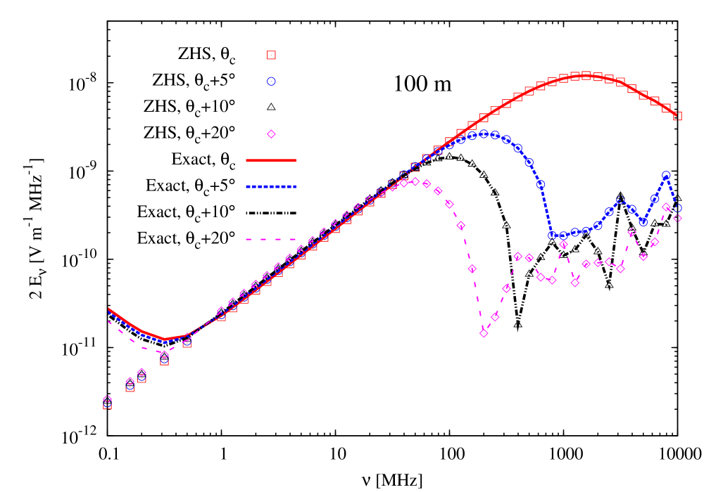
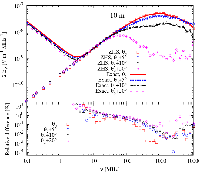
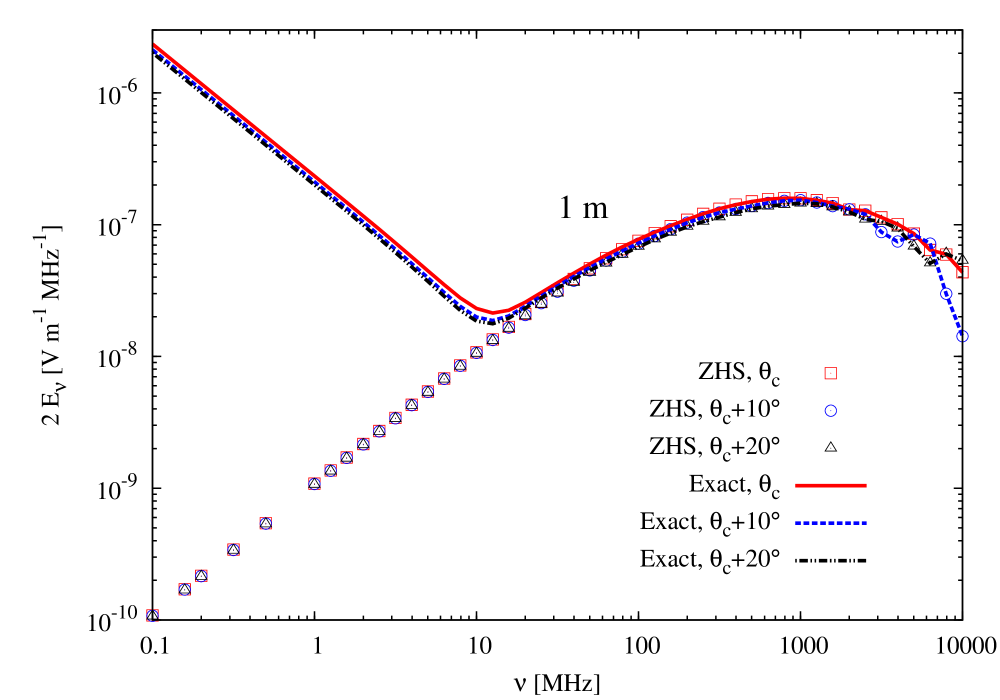
Figure 6: Fourier components of the electric field modulus as obtained in Monte Carlo simulations of a 10 TeV electron-induced shower in ice, with the exact calculation (lines) and with the ZHS algorithm (symbols). The field is shown for observers at distances (from top to bottom panels) $R=100$, 10, 1 m, placed at different observation angles with respect to shower maximum. In the middle panel corresponding to $R=10$ m, we also show the relative difference (in $\%$) between the electric field modulus as obtained with the exact solution and with the ZHS algorithm for the various observation angles depicted.

V Comparison to other calculations

Several calculations of the field emitted in showers developing in dense media can be found in the literature. In Chih10 the Finite Diference Time Domain method is used for calculating the field of a pancake-like shower with a Gaussian longitudinal development and Gaussian radial profile in the time-domain which is then transformed to the frequency-domain. In buniy02 using the saddle-point approximation, an analytic equation for the calculation of the electric field of a charge distribution exhibiting a longitudinal profile with a well-pronounced maximum is derived. The result is factorized into an integral accounting for the longitudinal variation of the charge and a form factor that accounts for the lateral spread of the shower, a procedure revisited in ARZ11 for realistic showers. Assuming a Gaussian longitudinal and lateral development for the charge distribution both results were directly compared and turned out to be in good overall agreement as shown in Chih10 . Minor differences could be attributed to the form factors used.

With the exact calculation of the electric field performed in this work, the field due to a Gaussian profile can also be obtained and compared to the calculations mentioned before. The electric current for a shower with a Gaussian profile is given by Eq. (1) with the following replacements:

$$Z(t)=1$$ (40)

and

$$P(\mathbf{x},t)=\frac{N}{2\pi\sigma_{r}^{2}}~{}e^{-(x^{2}+y^{2})/2\sigma_{r}^{2}}~{}e^{-z^{2}/2\sigma_{l}^{2}}\delta(z-vt)$$ (41)

The shower develops in the longitudinal direction parallel to the $z^{\prime}$ coordinate (shower axis), and radially along the $x^{\prime}$ and $y^{\prime}$ coordinates. $N$ is a normalization constant. $\sigma_{l}$ characterizes the width of the shower along shower axis and $\sigma_{r}$ the corresponding lateral width. After substituting this current in Eq. (7), and following the same steps as in Section II.1, the expression for the field is the same as in Eqs. (11) and (12) with the following change:

$$\int\mathrm{d}t^{\prime}\ \ \rightarrow\ \ \int\mathrm{d}t^{\prime}\ \mathrm{d}x^{\prime}\ \mathrm{d}y^{\prime}\frac{N}{2\pi\sigma_{r}^{2}}~{}e^{-(x^{\prime 2}+y^{\prime 2})/2\sigma_{r}^{2}}~{}e^{-v^{2}t^{\prime 2}/2\sigma_{l}^{2}}$$ (42)

Eqs. (11) and (12) after the changes in Eq. (42) can be solved numerically. The ZHS algorithm can also be applied to this situation as long as the condition $kr\gg 1$ for all distances $r$ to the shower. The procedure consists on slicing the volume occupied by the bulk of the shower in small cubes and approximating each as a track with constant charge given by the Gaussian distributions in Eq. (41).

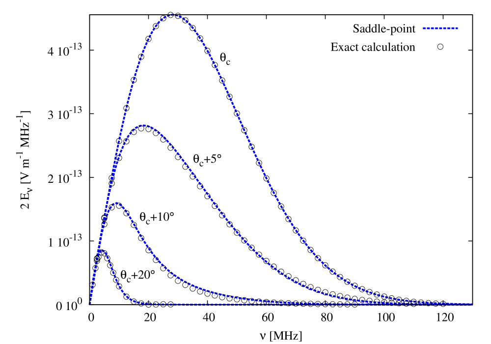
Figure 7: Fourier components of the modulus of the electric field for a Gaussian charge profile given in Eq. (41) with $\sigma_{l}=20$ m and $\sigma_{r}=1$ m for an observer at $R=300$ m with respect to the peak of the Gaussian longitudinal profile. The observation angles are, from top to bottom, $\theta_{C}$, $\theta_{C}+5^{\circ}$, $\theta_{C}+10^{\circ}$, and $\theta_{C}+20^{\circ}$. Fields are calculated with the saddle-point approach and the exact formula Eqs. (11) and (12). The result obtained with the ZHS algorithm is on top of the exact calculation and it is not plotted in the Fig. for clarity.

Comparison of the result of the exact calculation in this work (or the ZHS algorithm) with the saddle-point calculation in buniy02 requires knowing the form factor $F$ for a Gaussian profile. $F$ is defined in buniy02 as:

$$F(\mathbf{q})=\int\mathrm{d}x^{\prime}\mathrm{d}y^{\prime}\mathrm{d}s^{\prime}\ e^{-i\mathbf{q}\cdot\mathbf{x^{\prime}}}f(s^{\prime},x^{\prime},y^{\prime})$$ (43)

with $\mathbf{q}=(\omega/v,k\mathbf{\rho}/R)$ with $\mathbf{\rho}=(x,y)$ the radial position of the observer. Also, $\mathbf{x}^{\prime}=(s^{\prime},x^{\prime},y^{\prime})$ with $s^{\prime}=z^{\prime}-vt^{\prime}$. $R$ is the distance from the maximum of the shower to the observer. The function $f$ represents a normalized charge density of the travelling pancake. Assuming a Gaussian for $f$ of the form:

$$f(s^{\prime},x^{\prime},y^{\prime})=\frac{1}{2\pi\sigma_{r}^{2}}\delta(s^{\prime})~{}e^{-(x^{\prime 2}+y^{\prime 2})/2\sigma_{r}^{2}},$$ (44)

and substituting $f$ into Eq. (43), the form factor reads,

$$F(\mathbf{q})=e^{-\frac{1}{2}(\frac{n\omega}{c}\frac{\rho}{R}\sigma_{r})^{2}}$$ (45)

Setting $N=1$, $\sigma_{l}=20$ m, $\sigma_{r}=1$ m and $R=300$ m with the refractive index of ice $n=1.78$, the electric fields for a Gaussian charge profile were calculated using the saddle-point approach as described in buniy02 , and compared to the exact formula given in this work. The results are shown in Fig. 7. Since $R$ is large the condition $kR\gg 1$ is satisfied for frequencies above $\nu\sim 1$ MHz (see Eq. 36) and the agreement between the ZHS and the exact calculation presented in this work is very good (not shown in Fig. 7 for clarity). The saddle-point approach is also in very good agreement with both the exact and ZHS calculations. The results of the field for a Gaussian charge profile are also in good agreement with those obtained in Chih10 using the Finite Difference Time Domain method.

VI Summary and conclusions

We have obtained the results of an exact calculation of the electric field produced by a charged particle that accelerates instantaneously moves at constant speed and intantaneously deccelerates. The results are used to obtain the approximate expression used in the ZHS algorithm to calculate the radio emission from showers in dense media using shower simulations. This allows the precise determination of the conditions necessary for this approximation to be valid, namely, the observer must be in the far field zone $kR\gg 1$ and the Frauhofer approximation must apply, $kL^{2}\sin^{2}\theta/R\ll 1$ for each track. The exact and simulated results are compared for tracks in a variety of circumstances to illustrate both the behavior of the fields and the validity of the approximation made in different frequency and distance ranges.

We have shown that the range of validity of the expressions can be greatly enlarged by subdividing long charged particle tracks in smaller sub-tracks and adding up the conributions, as it is done in the ZHS algorithm. Nevertheless the far field condition $kR\gg 1$ has been shown to be an intrinsic limit of the ZHS algorithm. The ZHS algorithm has been tested for long tracks in regions where the Fraunhofer approximation does not hold comparing it to the exact solution. The results clearly indicate that the ZHS algorithm reproduces the exact behavior provided the far field condition is satisfied and the length of the sub-tracks is small enough for the Fraunhofer approximation to be valid. By comparing the emission with the exact emission from an infinite track it is shown that the emission calculated with the ZHS algorithm does indeed contain what is conventionally described as Cherenkov radiation. The precision of the ZHS algorithm is shown to be below the $2\%$ level provided that $kR>3.7$, corresponding to $R>10$ m and $\nu>10$ MHz. By enforcing $kR>37$ the precision improves to better than $0.01\%$, what corresponds to $R>10$ m and $\nu>100$ MHz, which are conditions met in most experimental arrangements trying to detect radio pulses form neutrinos interacting in dense media.

The ZHS algorithm is tested for completitude when applied to a shower simulation. This is done comparing the result of the ZHS algorithm to that obtained when the ZHS expression is replaced by the exact calculation for every charged particle sub-track for exactly the same shower. The results indeed confirm that the accuracies reported for individual sub-tracks are approximately mantained in the final ZHS result.

Finally, in order to compare to alternative calculations the results are compared to the saddle point approximation. This approximation has been used to test solutions using the method of Finite Differences to solve Maxwell’s Equations directly in the Time Domain (FDTD) using a simplified shower front based on gaussian distributions in the shower plane and in time. The comparison of the saddle point approximation to both the exact solution and the ZHS algorithm give compatible results confirming that both approaches reproduce the radiation emitted from showers.

The results presented here in summary confirm that the ZHS algorithm can be used to describe most practical applications to detect pulses emitted from high energy showers produced in dense media by neutrinos. The approach only begins to show significant discrepancies when the observer is at distances comparable to the lateral dimensions of the shower ($\lesssim$ 1 m in ice). Since the typical distance between antennas in experiments such as the Askaryan Radio Array (ARA) ARA is $\sim 10-100$ m, we expect the results to be accurate enough in most practical situations.

The results obtained are also of interest for the application of the ZHS algorithm to calculate pulses from EAS. Indeed the application of the method of track subdivision has been applied in ZHAireS ZHAireS_air , a recent code developed for this purpose, by making track subdivisions that are forced to satisfy the Fraunhofer condition.

VII Acknowledgments

J.A-M, W.R.C., D.G.-F. and E.Z. thank Xunta de Galicia (INCITE09 206 336 PR) and Consellería de Educación (Grupos de Referencia Competitivos – Consolider Xunta de Galicia 2006/51); Ministerio de Educación, Cultura y Deporte (FPA 2010-18410, FPA2012-39489 and Consolider CPAN - Ingenio 2010); ASPERA (PRI-PIMASP-2011-1154) and Feder Funds, Spain. We thank CESGA (Centro de SuperComputación de Galicia) for computing resources. Part of this research was carried out at the Jet Propulsion Laboratory, California Institute of Technology, under a contract with the National Aeronautics and Space Administration.

References

- (1) R.U. Abbasi et al. [HiRes Collaboration] Phys. Rev. Lett. 100, 101101 (2008)
- (2) J. Abraham et al. [Pierre Auger Collaboration], Phys. Rev. Lett. 101, 061101 (2008); J. Abraham et al. [Pierre Auger Collaboration], Physics Letters B 685, 239 (2010).
- (3) J. Abraham et al. [Pierre Auger Collaboration], Phys. Rev. Lett. 104, 091101 (2010)
- (4) R.U. Abbasi et al. [HiRes Collaboration] Phys. Rev. Lett. 104, 161101 (2010)
- (5) K. Kotera, A. Olinto, JCAP 10, 013 (2010).
- (6) G.A. Askar’yan, Soviet Physics JETP 14,2 441–443 (1962); 48 988–990 (1965).
- (7) J.V. Jelley, Nuovo Cimento X 46, 649 (1966).
- (8) H. R. Allan, in: J. G. Wilson, S. A. Wouthuysen (Eds.), Progress in Elementary Particle and Cosmic Ray Physics, North Holland, (1971), p. 169.
- (9) D. Saltzberg et al., Phys. Rev. Lett. 86, 2802 (2001).
- (10) P. Miocinovic et al. Phys. Rev. D 74, 043002 (2006).
- (11) P.W. Gorham et al. Phys. Rev. D 72, 023002 (2005).
- (12) P.W. Gorham et al. Phys. Rev. Lett. 99, 171101 (2007).
- (13) E. Zas, F. Halzen, T. Stanev, Phys. Rev. D 45, 362 (1992).
- (14) I. Kravchenko et al., Astropart. Phys. 19, 15 (2003); I. Kravchenko et al. [RICE Collaboration], Phys. Rev. D 85, (2012) 062004.
- (15) P.W. Gorham et al. [ANITA Collaboration], Astropart. Phys. 32, (2009) 10; P.W. Gorham et al. Phys. Rev. Lett. 103, 051103 (2009); P.W. Gorham et al. [ANITA Collaboration], Phys. Rev. D 82, (2010) 022004; Phys. Rev. D 85, (2012) 049901(E).
- (16) T. Hankins et al. Mon. Not. Royal Astron. Soc. 283, 1027 (1996).
- (17) P.W. Gorham et al. Phys. Rev. Lett. 93, 041101 (2004).
- (18) O. Scholten et al. Astropart. Phys. 26, 219 (2006).
- (19) A.R. Beresnyak et al. Astronomy Reports 49 2, 127 (2005).
- (20) C.W. James et al. Phys. Rev. D 81, 042003 (2010).
- (21) T.R. Jaeger, R.L. Mutel, K.G. Gayley, Astropart. Phys. 34, 293 (2010).
- (22) P. Allison et al. [ARA Collaboration] Astropart. Phys. 35, (2012) 457
- (23) S.W. Barwick et al. J. Phys. Conf. Ser. 60, 276-286 (2007).
- (24) S. Fliescher for the Pierre Auger Collaboration, Nucl. Instrum. Meth. A 662, S124 (2012)
- (25) D. Ardouin et al., Astropart. Phys. 31, 192 (2009).
- (26) S. Hoover et al. [ANITA Collaboration], Phys. Rev. Lett. 105, 151101 (2010).
- (27) P.W. Gorham, F.E. Baginski, P. Allison, K.M. Liewer, C. Miki, B. Hill, G.S. Varner, Astropart. Phys. 35 242, (2011)
- (28) F. Halzen, E. Zas, T. Stanev, Phys. Lett. B 257, 432 (1991).
- (29) J. Alvarez-Muñiz, E. Zas, Phys. Lett. B 411, 218 (1997).
- (30) J. Alvarez-Muñiz, E. Zas, Phys. Lett. B 434, 396 (1998).
- (31) J. Alvarez-Muñiz, R.A. Vázquez and E. Zas, Phys. Rev. D 61, 023001 (1999).
- (32) J. Alvarez-Muñiz, R.A. Vázquez, E. Zas, Phys. Rev. D 62, 063001 (2000).
- (33) S. Razzaque et al. Phys. Rev. D 65, 103002 (2002);
- (34) J. Alvarez-Muñiz, E. Marqués, R.A. Vázquez, E. Zas, Phys. Rev. D 67, 101303 (2003).
- (35) S. Razzaque et al. Phys. Rev. D 69, 047101 (2004).
- (36) S. Hussain, D.W. McKay, Phys. Rev. D 70, 103003 (2004).
- (37) J. Alvarez-Muñiz, E. Marqués, R.A. Vázquez, E. Zas, Phys. Rev. D 74, 023007 (2006).
- (38) J. Alvarez-Muñiz, C.W. James, R.J. Protheroe and E. Zas, Astropart. Phys. 32, 100 (2009).
- (39) J. Alvarez-Muñiz, A. Romero-Wolf, E. Zas, Phys. Rev. D 81, 123009 (2010).
- (40) J. Alvarez-Muñiz, W. Rodrigues, M. Tueros and E. Zas, Astroparticle Physics 35, 287 (2012)
- (41) J. Alvarez-Muñiz, A. Romero-Wolf, E. Zas, Phys. Rev. D 84, 103003 (2011)
- (42) J. Alvarez-Muñiz, W. Rodrigues, M. Tueros and E. Zas, Astroparticle Physics 35, 325 (2012)
- (43) I. Tamm, Journal of Physics I, No. 5-6, 439 (1939)
- (44) J.D. Jackson, Classical Electrodynamics 3rd Ed. Wiley, New York, (1998).
- (45) C.W. James, H. Falcke, T. Huege, and M. Ludwig Phys. Rev. E 84, 056602 (2011)
- (46) R.V. Buniy, J.P. Ralston, Phys. Rev. D 65, 016003 (2002).
- (47) C.-Y. Hu, C.-C. Chen, P. Chen, Astroparticle Physics 35, 421 (2012).
- (48) J. Alvarez-Muñiz, G. Parente, E. Zas, in Procs. of the 24th ICRC, Rome (Italy), Vol. 1, 1023 (1995).
- (49) G.N. Afanasiev, Vavilov-Cherenkov and synchrotron radiation: foundations and applications, Kluwer Academic Publishers, (2004)