Networks of quantum wire junctions: a system with quantized integer Hall resistance without vanishing longitudinal resistivity

Abstract

We consider a honeycomb network built of quantum wires, with each node of the network having a Y-junction of three wires with a ring through which flux can be inserted. The junctions are the basic circuit elements for the network, and they are characterized by $3\times 3$ conductance tensors. The low energy stable fixed point tensor conductances result from quantum effects, and are determined by the strength of the interactions in each wire and the magnetic flux through the ring. We consider the limit where there is decoherence in the wires between any two nodes, and study the array as a network of classical 3-lead circuit elements whose characteristic conductance tensors are determined by the quantum fixed point. We show that this network has some remarkable transport properties in a range of interaction parameters: it has a Hall resistance quantized at $R_{xy}=h/e^{2}$, although the longitudinal resistivity is non-vanishing. We show that these results are robust against disorder, in this case non-homogeneous interaction parameters $g$ for the different wires in the network.

I Introduction

The transport properties of junctions of quantum wires are of interest both seen from basic and applied perspectives. From the basic physics aspect, quantum wires provide experimentally realizable ways for studying interacting electrons in one-dimensional geometries, and in particular junctions where 3 or more wires meet can display rather rich behaviors. Theoretically, the problem of quantum wire junctions is related to dissipative quantum mechanics in two or higher dimensions, and to boundary conformal field theory. Chamon et al. (2003); Oshikawa et al. (2006) It also has a mathematical connection to certain aspects of open string theory in a background magnetic field. Callan et al. (1995); Callan and Freed (1992) From a practical viewpoint, junctions of quantum wires should serve as important building blocks for the integration of quantum circuits, as they are the natural element to split electric signals and serve as interconnects.

Junctions of quantum wires have been the subject of many recent studies, Nayak et al. (1999); Lal et al. (2002); Chamon et al. (2003); Chen et al. (2002); Pham et al. (2003); Rao and Sen (2004); Kazymyrenko and Douçot (2005); Oshikawa et al. (2006); Bellazzini et al. (2007); Hou and Chamon (2008); Das and Rao (2008); Agarwal et al. (2009); Bellazzini et al. (2009a, b); Safi (2009); Aristov et al. (2010); Mintchev (2011); Aristov (2011); Aristov and Wölfle (2011); Wang and Feldman (2011); Caudrelier et al. (2012) which have uncovered many interesting transport properties as function of interaction strength. Quantum wires with few transport channels, at low energies, can be described as Tomonaga-Luttinger liquids, characterized by a Luttinger parameter $g$ which encodes the electron-electron interactions. Tomonaga (1950); Luttinger (1963); Mattis and Lieb (1965); Haldane (1981) The transport properties of a given junction depends on the Luttinger parameters for each wire. At low energies, the conductance properties of the junctions of $n$ wires are encoded in an $n\times n$ conductance tensor or matrix $G_{jk}$ that relate the incoming currents to the applied voltages on the wires via $I_{j}=\sum_{k}G_{jk}\,V_{k}$. At low voltages and low temperatures, the tensor takes universal forms dictated by the nature of the infrared stable fixed points in the renormalization group (RG) sense. These fixed points have been categorized for the case of Y-junctions ($n=3$) of spinless Oshikawa et al. (2006) and spinful Hou and Chamon (2008) electrons as function of the interaction parameter $g$ when all the wires are identical, and more recently in the case when the wires are not identical and have different values $g_{i}$. Hou et al. (2012)

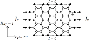
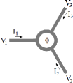
Figure 1: (a) Scheme of a grid showing the flow of the current and the boundary conditions. External currents are fixed, as well as the potential on the node on the upper right corner. (b) Building block of the grid: junction of three quantum wires with a magnetic flux threading the ring. The $V_{1,2,3}$ are the voltages applied on each wire, and the $I_{1,2,3}$ the currents arriving at the junction from each of the three wires.

In this paper we investigate the transport properties of networks constructed using Y-junctions of quantum wires as building blocks. Fig. 1a depicts an example of a network shaped in the form of a rectangle, and Fig. 1b shows the individual Y-junctions used in each node. We consider a simplified model where the $3\times 3$ conductance tensor for each Y-junction is taken to be that dictated by the low energy quantum RG fixed point, but the transport is treated classically between any two junctions. The treatment is sensible if the segment of the wires between two junctions is large compared to the characteristic dephasing length in the system. But the length scales of the junction itself, for example the size of a ring as shown in Fig. 1b, should be smaller than the dephasing length so that the junction is treated quantum mechanically. The case when the full system is treated quantum mechanically is extremely difficult to analyze, because it is an interacting problem. For instance, a lattice version of the problem would essentially be an example of a two-dimensional interacting lattice model with a fermion sign problem.

We find rather remarkable results for the transport characteristics of the network of Y-junctions, even when the role of quantum mechanics is just to select the RG stable fixed point conductances of the elementary building blocks. When the conductance is controlled by the chiral fixed points $\chi_{\pm}$, Chamon et al. (2003); Oshikawa et al. (2006) we find that the whole network behaves as a Hall bar, with a Hall resistance that is quantized to $R_{xy}=\pm h/e^{2}$, like in the integer quantum Hall effect, with the sign given by the particular chirality of the fixed points $\chi_{+}$ or $\chi_{-}$. However, the longitudinal resistivity $\rho_{xx}\neq 0$, unlike in the case of the quantized Hall effect where $\rho_{xx}$ vanishes. The quantization of $R_{xy}$ is a manifestation of the universal fixed point conductances. The chiral fixed points are stable for a range of Luttinger parameters $1<g<3$, and which of $\chi_{+}$ or $\chi_{-}$ is selected depends on the flux threading the ring in the Y-junction. Chamon et al. (2003); Oshikawa et al. (2006) The flux breaks time-reversal symmetry, but it does not need to be quantized at any given value; because of interactions, the conductance of the Y-junction flows to fixed point values for a range of fluxes.

The quantization of $R_{xy}=\pm h/e^{2}$ for the network as a whole is independent of the value of $g$ in the wires, as long as they are in the range of stability of the chiral fixed points. Moreover, we show that the quantization $R_{xy}=\pm h/e^{2}$ is stable against disorder in the wire parameters. Specifically, we show that the quantization of $R_{xy}$ remains even when the values of $g$ for different wires are not uniform but disordered, i.e., they are randomly distributed around some average value $g$ with some spread $\delta g$.

The paper is organized as follows. In Sec. II we briefly review the results for the conductance characteristics of single quantum Y-junctions, which are the elementary building blocks for the honeycomb wire-networks. In Sec. III we present analytical results from which one can understand the origin of the quantization of $R_{xy}$ when the conductance tensor of each of the Y-junctions in the network is associated to a chiral fixed point. In Sec. IV we present numerical studies confirming the analytical findings by analyzing grids with different values of the interaction parameter $g$, different geometries and sizes, and extrapolate these results to the thermodynamic limit. These numerical calculations are of much value for the next step, taken in Sec.  V, where we discuss the robustness of the quantization of the Hall resistance in the case when the wires each have different Luttinger parameters distributed randomly. The Appendix contains a detailed description of the numerical method to solve our network of Y-junctions.

II Single Y-junction as elementary circuit element

Each of these Y-junctions in the network consists of three wires that are connected to a ring which can be threaded by a magnetic flux, as shown in Fig. 1b. This flux breaks time-reversal symmetry, and the currents in the junction will depend on the potential at its extremes and the magnetic flux inside the junction.

The current-voltage response of each Y-junction is determined by its conductance tensor $G_{jk}$. Within linear response theory, the total current $I_{j}$ flowing into the junction from wire $j$ is related to the voltage $V_{k}$ applied to wire $k$ by

$$I_{j}=\sum_{k}G_{jk}V_{k}$$ (1)

where $j,k=1,2,3$. Two sum rules apply to the conductance tensor because of conservation of current and because the currents are unchanged if the voltages are all shifted by a constant:

$$\sum_{j}G_{jk}=\sum_{k}G_{jk}=0\;.$$ (2)

The $G_{jk}$ reach universal values at low temperatures and low bias voltages. These universal values are dictated by the RG stable fixed point that is reached for given values of the Luttinger parameters in the wires. Here we shall focus on the case where all the three wires have the same parameter $g$. In Sec. V we will consider the more general case of network of wires where the three wires for each Y-junction have different $g$’s.

When the three wires have the same $g$, the fixed point conductance tensor has a $Z_{3}$ symmetry and takes the form Oshikawa et al. (2006)

$$G_{jk}=\frac{G_{S}}{2}(3\delta_{jk}-1)+\frac{G_{A}}{2}\epsilon_{jk}\;,$$ (3)

where $\epsilon_{ij}=\delta_{i,j-1}-\delta_{i,j+1}$ with $i+3\equiv i$ and we separate the symmetric and anti-symmetric components of the tensor, whose magnitudes are encoded in the scalar conductances $G_{S}$ and $G_{A}$. $G_{A}$ vanishes when time-reversal symmetry is not broken, for instance in the absence of magnetic flux through the ring.

The fixed point values of $G_{S}$ and $G_{A}$ depend on the strength of electron-electron interactions, encoded in the Luttinger parameter $g$. We will focus on the chiral fixed points $\chi_{\pm}$, which are stable in the range $1<g<3$. Chamon et al. (2003); Oshikawa et al. (2006) In the chiral cases, the conductances are given by $G_{S}=G_{\chi}=\frac{e^{2}}{h}\frac{4g}{3+g^{2}}$ and $G_{A}=\pm g\,G_{\chi}$. Thus the chiral conductance tensors are:

$$G_{jk}^{\pm}=\frac{G_{\chi}}{2}[(3\delta_{jk}-1)\pm g\epsilon_{jk}]\;.$$ (4)

We shall work in units where the quantum of conductance $e^{2}/h$ is set to 1.

The Y-junctions are then assembled into a network as shown in Fig. 1a. We consider a regular hexagonal grid of Y-junctions with $2c$ external connections on both the top and bottom sides and $r$ on both the right and left side. Parametrized in such a way and with wires of unit length, the dimensions of the grid as a function of $r$ and $c$ are

$$L_{x}=6c$$

$$L_{y}=\sqrt{3}(2r+1)\;.$$ (5)

In this grid we shall fix the current flow along the $x$-axis from left to right and we shall fix the currents flowing into the top and the bottom to zero, as shown in Fig. 1a. Given the conductance tensors at every node of the network, we compute the potentials and the currents on the links of the grid. The resistances and resistivities of the networks are studied for different orientations and systems sizes, and for different values of $g$. In appendix A we present details of the method used to numerically compute the response of the networks.

III Analytical Results

We will measure the longitudinal and transverse responses in the framework of the classical Hall problem by injecting a transverse current along the $x$-axis and imposing a zero current boundary condition along the two edges that are parallel to the $x$-axis. This approach suggests that we solve for the potential in the bulk as a function of the external current. In other words we need to invert the fundamental equation (1) for $I$ and $V$ for each junction in the bulk.

While the full network problem is not tractable analytically, we can still gain some insight from a combination of analytics and heuristics. In particular we will be able to prove quantization of the transverse resistivity analytically, even with some forms of disorder. Similarly we will derive the general form of the longitudinal resistivity. We will confirm these results numerically in later sections. Let us start with the unit cell of the hexagonal lattice. There are two vertices (nodes) in each cell and current is directed along the bonds (wires) as shown in Fig. 2. Looking at the right-hand node first, the potentials on the external wires, $V_{2}$ and $V_{3}$, and the potential on the internal wire $V_{1}$ are defined only up to an additive constant. This means that Eq. (1) is not invertible. However, by setting $V_{1}=0$, or equivalently shifting all potentials in the two nodes by a constant $V_{i}\rightarrow V_{i}-V_{1}$, the gauge is fixed and we obtain, using Eq. (4), the following:

$$\begin{pmatrix}V_{2}-V_{1}\\ V_{3}-V_{1}\end{pmatrix}=\frac{1}{2g}\begin{pmatrix}2&1\mp g\\ 1\pm g&2\end{pmatrix}\begin{pmatrix}I_{2}\\ I_{3}\end{pmatrix}\;.$$ (6)

The solution in the left node is similar but with the permutation $(V_{2},V_{3})\rightarrow(V^{\prime}_{2},V^{\prime}_{3})$ and $(I_{2},I_{3})\rightarrow-(I^{\prime}_{2},I^{\prime}_{3})$, which follows from rotational symmetry and the orientation that we have chosen for the currents.

Figure 2: Unit cell of the hexagonal network. Currents are assumed to be positive when directed along the arrows in the wires. Dotted lines denote the boundary of the unit cell. The rectangular region $ABCD$ shown is used for computing the resistances and resistivities of the network.

Now consider the potential gradient in the $x-$ and $y-$directions. It is straightforward to derive the change in potential per unit cell, $\Delta V_{x}$ and $\Delta V_{y}$, directly from Eq. (6) as follows:

$$\Delta_{x}V=V^{\prime}_{3}-V_{2}=\frac{1}{2g}\left[2I_{1}-I_{2}-I^{\prime}_{3}\mp g\left(I^{\prime}_{2}-I_{3}\right)\right]$$

$$\Delta_{y}V=V_{2}-V_{3}=\frac{1}{2g}\left[\pm gI_{1}+I_{2}-I_{3}\right].$$ (7)

It is instructive to consider a simple case. We will generalize this result below, but for now consider a uniform current in the bulk in the $x-$direction (or “armchair” configuration to borrow nomenclature from graphene). Each horizontal wire in each unit cell has a current $I_{1}=I$. By symmetry the other wires split the current equally: $I_{2}=I_{3}=I^{\prime}_{2}=I^{\prime}_{3}=-I/2$. This configuration leads to a particularly simple potential gradient: $\Delta_{x}V=3I/2g$ and $\Delta_{y}V=\pm I/2$.

The result for the resistances and resistivities are apparent after we account for the geometric factors. Consider the rectangular region $ABCD$ in Fig. 2, with sides $d_{AB}=\sqrt{3}$ and $d_{AD}=2$. In the transverse direction the width of the rectangle is twice the distance between the midpoint of the wires (with currents $I_{2}$ and $I_{3}$), and the voltage drop $V_{AB}=2\,\Delta_{y}V$. The Hall resistance (which coincides with the Hall resistivity $\rho_{xy}$) is therefore $R_{xy}=V_{AB}/I=2\,\Delta_{y}V/I=\pm 1$. In other words the Hall resistance is independent of $g$ and quantized to unity!

Similarly, in the longitudinal direction the length of the rectangle is 4/3 the distance between the midpoint of the wires (with currents $I^{\prime}_{2}$ and $I_{3}$), and $V_{AD}=4/3\,\Delta_{x}V$. The longitudinal resistance is $R_{xx}=4/3\,\Delta_{x}V/I=2/g$. There is an additional geometric factor in the longitudinal resistivity given by $\rho_{xx}=(d_{AB}/d_{AD})\,R_{xx}$, and it is thus given by $\rho_{xx}=\sqrt{3}/g$. Hence the resistivity is non-zero and there is dissipation unlike in the standard quantum Hall effect.

Had we used an alternate (“zigzag”) configuration where the transverse current is zero $I_{1}=0$ and the uniform current is in the $y-$direction, $I_{3}=I^{\prime}_{3}=-I_{2}=-I^{\prime}_{2}=I$, we would have found a similar result, i.e., that the resistance in the $x-$direction is quantized to $R_{xy}=\pm 1$ while the resistivity in the $y-$ direction is $\rho_{yy}=\sqrt{3}/g$.

We find this result both unexpected and remarkable. By taking the classical conductivity limit for each wire we have allowed decoherence along the wires. However we have preserved the quantum coherence on each vertex, as the chiral relation Eq. (4) is by nature a consequence of quantum scattering. Nonetheless even after relaxing a portion of the coherence, some element of quantization in the thermodynamic limit has survived in the form of an integer quantized Hall resistivity. On the other hand, decoherence has destroyed the zero longitudinal resistivity of the quantum Hall effect, and so we are left with a hybrid quantum-classical Hall effect. Note also that the simple uniform solution above suggests robustness against disorder, another element of the integer quantum Hall effect. As the transverse gradient of $V$ is independent of $g$ in the uniform bulk, suppose that $g$ is allowed to vary slowly from vertex to vertex, more slowly than the current. In this regime we would expect quantization to persist, and indeed we will confirm that numerically later in this paper.

We will substantiate the assumptions and findings above numerically in the next section.

IV Numerical results

In this section we shall present numerical results for the voltages and currents in the wires of the network. These numerical studies serve first as a check of the analytical results presented in the previous section III for the case where all the interaction parameters are the same for all wires. Second, and more importantly, they serve as a stepping stone to the case of non-homogeneous (disordered) interaction parameters in the wires, which will be considered in Sec. V. The method used to solve for the voltages and currents in the grid is presented in Appendix A.

Let us focus on the armchair layout of Fig. 1a (similar results follow in the case of the zigzag case). Also, without loss of generality, we consider below only the $\chi_{+}$ fixed point. Current is injected and collected uniformly into the wires on the right and on the left of the network, respectively. More precisely, there are $r$ wires serving as connections to the outside on each side of the grid, and current $I=I_{x}/r$ is injected in and collected out of these external wires. The total current flowing along the horizontal or $x$-direction is therefore $I_{x}$.

The distribution of the currents in the inner parts of the grid that follow from this uniform injection of external currents is shown in Fig. 3. We find a close to uniform distribution, with slightly larger currents closer to the edges. This distribution is independent of the value of $g$. These patterns of current flow in the inner wires of the grid are in agreement with the current distributions discussed in the analytical studies of the previous section.

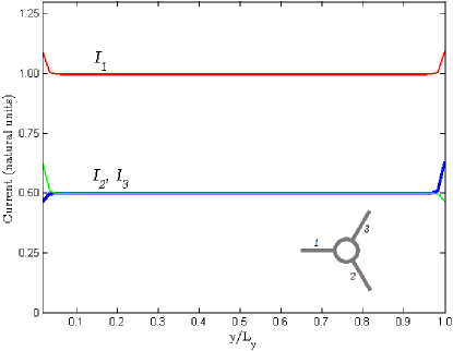
Figure 3: Currents flowing through the Y-junctions that lie along a vertical line in the middle of the bar ($x=L_{x}/2$) as a function of vertical position $y/L_{y}$. Note that for $y$ values away from the edges the currents tend to $I_{1}=1$ and $I_{2,3}=1/2$, as predicted analytically for the asymptotic limit.

The Hall voltage is the potential drop $V_{y}$ along the vertical or $y$-direction. We note that the potential drop $V_{y}$ is computed by looking at the potentials for two points at the same horizontal position (i.e., the same $x$ position), one at the top and one at the bottom of the network.

We show in Fig. 4 the potentials measured at the top and at bottom of the (rectangular shaped) grid. Notice that the potentials drop linearly with the horizontal direction, but that the difference between the two potentials, $V_{y}$, is constant.

The Hall resistance is computed as follows. Let $\bar{V}_{y}$ be the average over the horizontal positions $x$ of the Hall voltage drop. (Since in this case without disorder $V_{y}$ is constant, the average is actually unnecessary here.) Then the Hall resistance is given by $R_{xy}=\bar{V}_{y}/I_{x}$. We find numerically that $R_{xy}=1$ as expected from the analytical arguments.  Recall that we are working in units where $e^{2}/h=1$, so indeed we have

$$R_{xy}=\frac{h}{e^{2}}\;,$$ (8)

which we find is independent of the value of $g$. We remark that we find that this quantization holds independent of the aspect ratio, orientation (armchair vs. zigzag) or size of the grid.

We also computed the potential difference between points on the left and on the right sides of the grid, $V_{x}$, as a function of the vertical direction $y$. In this case we find that the horizontal potential difference is almost constant as function of $y$ (as opposed to the case of the vertical drop $V_{y}$, which is exactly independent of $x$). The difference is bigger, by an amount of order $1/L_{y}$, when $y$ is in the middle of the grid as compared to when $y$ is at the edges. We define $\bar{V}_{x}$ as the $y$-position averaged voltage difference between the left and right sides of the grid. The longitudinal resistance is given by $R_{xx}=\bar{V}_{x}/I_{x}$, and the longitudinal resistivity by $\rho_{xx}=L_{y}/L_{x}\;\bar{V}_{x}/I_{x}$.

We find that the longitudinal resistance is non-zero, in agreement with Sec. III. We find numerically, however, that there are finite system size corrections to the analytical predictions. We find that

$$R_{xx}(g,L_{x},L_{y})=\frac{\sqrt{3}}{g}\frac{L_{x}}{L_{y}-A(L_{x},L_{y})}\;,$$ (9)

where $A$ is a factor of order 1 that corrects for finite sizes. We find numerically that in the thermodynamic limit $A\to 1$ for the armchair configuration, whereas $A=0$ independent of system size in the zigzag case. Therefore, in the thermodynamic limit we obtain

$$\rho_{xx}=\lim_{L_{x},L_{y}\to\infty}\frac{L_{y}}{L_{x}}\;R_{xx}(g,L_{x},L_{y})=\frac{\sqrt{3}}{g}\;,$$ (10)

in agreement with the result in Sec. III.

The Hall angle $\theta_{H}$ is given by $\tan\theta_{H}=\rho_{xy}/\rho_{xx}$, and we naturally find, given the agreement with the results for $\rho_{xx}$ and $\rho_{xy}$ above, that

$$\tan\theta_{H}=\frac{g}{\sqrt{3}}$$ (11)

in the thermodynamic limit. This Hall angle can be visualized very naturally by plotting the voltages at the wires on the grid, as shown in Fig. 5. The Hall angle appears as the slope of the lines of constant voltage. These equipotential lines are straight in this example where all the wires have the same interaction parameter $g$; this is no longer the case when disorder is introduced in the next Sec. V.

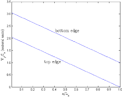
Figure 4: Voltages at the top and and bottom edges as function of horizontal position $x/L_{x}$ when the node at the top right corner is grounded. The grid size is $r=50$, $c=60$ and $g=\sqrt{3}$. Notice that the difference between the voltages at the top and bottom edges for a given $x/L_{x}$ is exactly 1 in natural units.

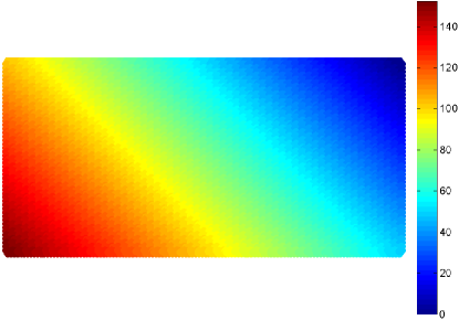
Figure 5: Density plot for the voltages on the grid nodes, for a system with $r=50$, $c=60$ and $g=\sqrt{3}$. Notice the constant slope of the equipotential lines, which is related to the Hall angle $\theta_{H}$. The Hall angle depends on the interaction strength and is given by Eq. 11.

V Robustness against disorder

In this section we will generalize the wire networks to the case when the interaction parameters $g$ for each of the wires in the network are not uniform, but instead are drawn independently from a distribution. We shall consider a distribution in which $g$ in each of the wires in the network takes a value between $(\bar{g}-\delta g,\bar{g}+\delta g)$, with uniform probability. Because the interaction parameter should be positive, $\delta g<\bar{g}$.

When the wires connecting to a given Y-junction have different values of $g$, the conductance tensor $G_{ij}$ for a chiral fixed point is no longer given by Eq. (4), but instead it takes the form (see Ref. Hou et al., 2012)

$$G_{jk}=2\frac{g_{j}(g_{1}+g_{2}+g_{3})\delta_{jk}+g_{j}g_{k}(\pm g_{m}\epsilon_{jkm}-1)}{g_{1}g_{2}g_{3}+g_{1}+g_{2}+g_{3}}\;.$$ (12)

Using this conductance tensor, one can compute numerically (using the method of Appendix A) the voltages and currents in all wires of the network for a given realization of the disorder.

We shall show below that the quantization $R_{xy}=1$ of the Hall conductance that we found in the clean limit remains , in the thermodynamic limit, even in the presence of disorder. For a finite lattice, as one should expect, there are fluctuations that we quantify below for the armchair configuration.

We compute Hall resistance $R_{xy}$ (defined as the average of the voltage differences between top and bottom of the network, divided by the injected current) for several realizations of disorder and system sizes. For a fixed system size, we then find the disorder average $\overline{R}_{xy}$ and standard deviation $\Delta R_{xy}=\sqrt{\overline{R^{2}_{xy}}-{\overline{R}_{xy}}^{2}}$ of $R_{xy}$. We find that $\overline{R}_{xy}\to 1$ as the number of realizations increase, and that the standard deviation $\Delta R_{xy}\to 0$ as $L$ increases (we use lattices with $r=c=L$). We show in Fig. 6 the finite size scaling of the $\Delta R_{xy}$. That $\Delta R_{xy}\to 0$ in the thermodynamic limit means that the system is self-averaging, and therefore $R_{xy}\to 1$ independent of disorder in the thermodynamic limit. We conclude then that quantization is robust against disorder.

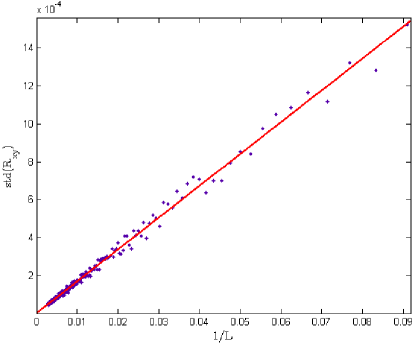
Figure 6: Standard deviation of the Hall resistance for 100 simulations with $\bar{g}=\sqrt{3}$ and $\delta g=\bar{g}/10$ as a function of $1/L$ for a grid with $r=c=L$ (which fixes the aspect ratio). It scales to zero in the large $L$ limit, implying that the system is self-averaging and the Hall resistance $R_{xy}\to 1$ independent of disorder in the thermodynamic limit.

We have also checked the effects of disorder for the zigzag configuration, reaching similar conclusions that disorder does not alter the quantization of the conductance in the thermodynamic limit.

In summary, we find that, in the thermodynamic limit, the general results of the previous sections hold even in the presence of disorder.

VI Conclusions

We investigated the transport properties of hexagonal networks whose nodes are Y-junctions of quantum wires. In our model the $3\times 3$ conductance tensor for each Y-junction is dictated by the low energy RG fixed point, but the transport is treated classically between any two junctions. We find a surprising result: in spite of relaxing quantum coherence between the junctions, we find a quantized Hall resistance.

Specifically, in the regime where the junction conductance is controlled by the chiral fixed points $\chi_{\pm}$, Chamon et al. (2003); Oshikawa et al. (2006) (when the interaction parameter obeys $1<g<3$), the network exhibits a quantized Hall resistance: $R_{xy}=\pm h/e^{2}$. This quantization is similar to that in the integer quantum Hall effect. Further, the quantization is independent of the interaction parameter $g$ even in the presence of disorder in $g$. The quantization of the Hall resistance follows from the specific form of the conductance tensor at the RG stable chiral fixed point at each Y-junction. However, unlike in the quantized Hall effect, where the longitudinal resistivity vanishes, $\rho_{xx}$ is not zero: $\rho_{xx}=(\sqrt{3}/g)\,h/e^{2}$. Dissipation in the longitudinal direction is a result of decoherence within the wires. We emphasize that in our model the wires are classical, but the nodes remain quantum mechanical and the form of the conductance tensor $G$ at each junction is constrained by quantum scattering effects. The essential ingredient for the quantization of the Hall conductance is the value of the chiral fixed point conductance of the individual junctions.

Finally, let us comment on the finite temperature corrections to the value $R_{xy}=\pm h/e^{2}$ in the network. As opposed to the case of the quantum Hall effect where the quantization is exponentially accurate because of an energy gap, the quantization in the networks has a power law correction in $T$ because the wire networks are gapless. The quantization should be as accurate as the conductance tensor is close to that of the RG fixed point. The corrections to the conductance tensor scale as $T^{\Delta}$, where $\Delta=4g/(3+g^{2})$ is the scaling dimension of the leading irrelevant operator at the chiral fixed points. Chamon et al. (2003); Oshikawa et al. (2006)

Notice that the temperature scaling of the conductivity above should hold only under the assumption of decoherence within the wires. However, as temperature goes to zero, the coherence length increases, and therefore there is an implicit assumption of order of limits for the results in this paper to work as presented: the length of the wires should be taken to infinity before the limit of $T=0$ is taken. But it is natural to wonder whether the quantization that we found in this work should persist or not even if transport along the wires is always coherent. Indeed, one possibility is that in the coherent regime one might have quantization of the Hall conductance with vanishing longitudinal resistivity. However, to address this regime one would need to tackle the fully interacting two-dimensional fermionic model, which is beyond the scope of this paper. One route to follow could be to consider a lattice model where the wires are described by a tight binding model, with three wires coupled together at junctions by hopping matrix elements between them. One could possibly start with a non-interacting version of the model, where the chiral conductances used in this paper are obtained by fine tuning to the fixed point (since the non-interacting model is marginal and there is no RG flow). The problem then becomes one of electrons in a superlattice, with the number of bands scaling with the number of sites describing the wires within a supercell. The Hall conductance for this tight-binding model could be obtained by computing the Chern number of the filled bands. If the Hall conductance does not vanish in this model, it is only protected algebraically in temperature, as there would be “mini gaps” separating bands that scale inversely with the size of the wires, instead of true band gaps. Analyzing such model may shine some light on the problem of wire networks in the coherent regimes.

Appendix A Method

Our numerical approach consists of solving the full lattice model exactly. In this section we describe our methodology in detail.

Consider an arbitrary lattice with $r$ external wires on each side and $2c$ external wires at the top and bottom edges. An equal current will be injected into each of the $r$ wires on the left, and the $2c$ edge wires will have a current of zero. This defines the boundary conditions. A $2\times 2$ lattice is shown for example in Figure 7. For later convenience we include a row of $2c$ “ghost nodes”, shown as dotted lines at the top edge, but they are only there to facilitate the numbering scheme and no current will flow through them. Including the ghost nodes there are a total of $N=4c(r+1)$ nodes.

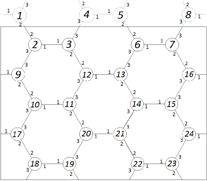
Figure 7: Example with $r=2$, $c=2$. Note the row of “ghost nodes” at the top edge.

The points on each wire that emanate from each node are governed by the equation $V=GI$ where $G$ is a $3\times 3$ matrix. Thus we start with $3N$ degrees of freedom. However, starting in this way introduces many redundant variables in the bulk because in a classical wire the current is the same everywhere along the wire and so is the potential. We will unify the two points on each wire in the bulk by imposing a set of constraints. In general there are $6cr+c-r$ such constraints, which equals the number of wires in the bulk.

To write down the full network equation let us label each of the $3N$ points by $(n,i)$, where $n=1,\dots,N$ is the node index and $i=1,2,3$ refers to the point on each wire that emanates from each node. The potentials and currents at each of these points are denoted by $V^{(n)}_{i}$ and $I^{(n)}_{i}$, respectively. To illustrate this notation, in Fig. 7 the constraint along the wire that connects nodes $6$ and $7$ would be written as $V^{(6)}_{1}=V^{(7)}_{1}$ and $I^{(6)}_{1}=-I^{(7)}_{1}$.

Each node obeys the relation $V^{(n)}=G^{(n)}I^{(n)}$ where $G^{(n)}$ is the $3\times 3$ matrix from Eq. (1). The network is thus described by the following linear equation with constraints:

$$\begin{pmatrix}I^{(1)}\\ I^{(2)}\\ \vdots\\ I^{(N)}\end{pmatrix}=\begin{pmatrix}G^{(1)}&0&\cdots&0\\ 0&G^{(2)}&\cdots&0\\ \vdots&\vdots&\ddots&\vdots\\ 0&0&\cdots&G^{(N)}\end{pmatrix}\begin{pmatrix}V^{(1)}\\ V^{(2)}\\ \vdots\\ V^{(N)}\;\end{pmatrix}$$ (13)

Next we impose the constraints to reduce the effective dimensionality of the problem. Start with the set of point pairs on each wire in the bulk $\{(n,i),(m,i)\}$, where $n$ and $m$ are nearest neighbor nodes. The constraints are $V^{(n)}_{i}=V^{(m)}_{i}$ and $I^{(n)}_{i}=-I^{(m)}_{i}$ for each pair. We impose the constraint on voltages by adding the $(n,i)$-th and $(m,i)$-th columns together, removing the $(m,i)$-th column and removing $V^{(m)}_{i}$ from the vector of potentials in Eq. (13). Similarly we impose the constraint on currents by adding the $(n,i)$-th and $(m,i)$-th rows, deleting the $(m,i)$-th row and removing $I^{(m)}_{i}$ from the vector of currents. Also we replace the current $I^{(n)}_{i}$ that has not been eliminated by zero because $I^{(n)}_{i}+I^{(m)}_{i}=0$. Therefore each constraint is equivalent to removing one row and one column and reduces the dimensionality of the original problem by one. Furthermore, we have replaced each current in the bulk by zero which is important because the only currents that are left in Eq. (13) are fully determined, being equal to either zero in the bulk or to the boundary conditions.

Eliminating the ghost nodes is straightforward – we simply remove the ghost currents, potentials and their associated rows and columns in Eq. (13). This reduces the dimensionality further by $3\times 2c$, which is the number of wires emanating from the ghost nodes. The final step is to fix the gauge. Since all potentials are determined up to an overall constant, we pick an arbitrary potential, set it to zero, and remove the associated row and column from Eq. (13).

To summarize, we started with $3N=12c(r+1)$ redundant degrees of freedom and then through successive transformations we imposed $6cr+c-r$ constraints in the bulk, eliminated $6c$ ghost points, and fixed one potential to zero. The dimensionality has thus been reduced to $6rc+5c+r-1$ and, crucially, the only currents appearing are either zero or fixed by boundary conditions. Having eliminated all redundancies allows us to solve for the potential at any point, as a function of the boundary currents, by inverting the reduced version of Eq. (13), which we do numerically.

The generalization to random couplings $g$ is straightforward. The derivation proceeds in exactly the same way as we just described, but we start with non-uniform $G^{(n)}$.

References

- Chamon et al. (2003) C. Chamon, M. Oshikawa, and I. Affleck, Phys. Rev. Lett. 91, 206403 (2003).
- Oshikawa et al. (2006) M. Oshikawa, C. Chamon, and I. Affleck, J. Stat. Mech.: Theory Exp. 2006, P02008 (2006).
- Callan et al. (1995) C. G. Callan, I. R. Klebanov, J. M. Maldacena, and A. Yegulalp, Nuclear Physics B 443, 444 (1995).
- Callan and Freed (1992) C. G. Callan and D. Freed, Nuclear Physics B 374, 543 (1992).
- Nayak et al. (1999) C. Nayak, M. P. A. Fisher, A. W. W. Ludwig, and H. H. Lin, Phys. Rev. B 59, 15694 (1999).
- Lal et al. (2002) S. Lal, S. Rao, and D. Sen, Phys. Rev. B 66, 165327 (2002).
- Chen et al. (2002) S. Chen, B. Trauzettel, and R. Egger, Phys. Rev. Lett. 89, 226404 (2002).
- Pham et al. (2003) K.-V. Pham, F. Piéchon, K.-I. Imura, and P. Lederer, Phys. Rev. B 68, 205110 (2003).
- Rao and Sen (2004) S. Rao and D. Sen, Phys. Rev. B 70, 195115 (2004).
- Kazymyrenko and Douçot (2005) K. Kazymyrenko and B. Douçot, Phys. Rev. B 71, 075110 (2005).
- Bellazzini et al. (2007) B. Bellazzini, M. Mintchev, and P. Sorba, Journal of Physics A: Mathematical and Theoretical 40, 2485 (2007).
- Hou and Chamon (2008) C.-Y. Hou and C. Chamon, Phys. Rev. B 77, 155422 (2008).
- Das and Rao (2008) S. Das and S. Rao, Phys. Rev. B 78, 205421 (2008).
- Agarwal et al. (2009) A. Agarwal, S. Das, S. Rao, and D. Sen, Phys. Rev. Lett. 103, 026401 (2009).
- Bellazzini et al. (2009a) B. Bellazzini, P. Calabrese, and M. Mintchev, Phys. Rev. B 79, 085122 (2009a).
- Bellazzini et al. (2009b) B. Bellazzini, M. Mintchev, and P. Sorba, Phys. Rev. B 80, 245441 (2009b).
- Safi (2009) I. Safi, arXiv:0906.2363 (2009).
- Aristov et al. (2010) D. N. Aristov, A. P. Dmitriev, I. V. Gornyi, V. Y. Kachorovskii, D. G. Polyakov, and P. Wölfle, Phys. Rev. Lett. 105, 266404 (2010).
- Mintchev (2011) M. Mintchev, Journal of Physics A: Mathematical and Theoretical 44, 415201 (2011).
- Aristov (2011) D. N. Aristov, Phys. Rev. B 83, 115446 (2011).
- Aristov and Wölfle (2011) D. N. Aristov and P. Wölfle, Phys. Rev. B 84, 155426 (2011).
- Wang and Feldman (2011) C. Wang and D. E. Feldman, Phys. Rev. B 83, 045302 (2011).
- Caudrelier et al. (2012) V. Caudrelier, M. Mintchev, and E. Ragoucy, arXiv:1202.4270 (2012).
- Tomonaga (1950) S. Tomonaga, Prog. Theor. Phys. 5, 544 (1950).
- Luttinger (1963) J. M. Luttinger, J. Math. Phys. 4, 1154 (1963).
- Mattis and Lieb (1965) D. C. Mattis and E. H. Lieb, J. Math. Phys. 6, 304 (1965).
- Haldane (1981) F. D. M. Haldane, J. Phys. C 14, 2585 (1981).
- Hou et al. (2012) C.-Y. Hou, A. Rahmani, A. E. Feiguin, and C. Chamon, Phys. Rev. B 86, 075451 (2012).