Resonances for large one-dimensional “ergodic” systems

Abstract.

The present paper is devoted to the study of resonances for one-dimensional quantum systems with a potential that is the restriction to some large box of an ergodic potential. For discrete models both on a half-line and on the whole line, we study the distributions of the resonances in the limit when the size of the box where the potential does not vanish goes to infinity. For periodic and random potentials, we analyze how the spectral theory of the limit operator influences the distribution of the resonances.

Résumé. Dans cet article, nous étudions les résonances d’un système unidimensionnel plongé dans un potentiel qui est la restriction à un grand intervalle d’un potentiel ergodique. Pour des modèles discrets sur la droite et la demie droite, nous étudions la distribution des résonances dans la limite de la taille de boîte infinie. Pour des potentiels périodiques et aléatoires, nous analysons l’influence de la théorie spectrale de l’opérateur limite sur la distribution des résonances.

0. Introduction

Consider $V:\ \mathbb{Z}\to\mathbb{R}$ a bounded potential and, on $\ell^{2}(\mathbb{Z})$, the Schrödinger operator $H=-\Delta+V$ defined by

$$(Hu)(n)=u(n+1)+u(n-1)+V(n)u(n),\quad\forall n\in\mathbb{Z},$$

for $u\in\ell^{2}(\mathbb{Z})$.
The potentials $V$ we will deal with are of two types:

• $V$ periodic;

• $V=V_{\omega}$, the random Anderson model, i.e., the entries of the diagonal matrix $V$ are independent identically distributed non constant random variable.

The spectral theory of such models has been studied extensively (see, e.g., [19]) and it is well known that

• when $V$ is periodic, the spectrum of $H$ is purely absolutely continuous;

• when $V=V_{\omega}$ is random, the spectrum of $H$ is almost surely pure point, i.e., the operator only has eigenvalues; moreover, the eigenfunctions decay exponentially at infinity.

Pick $L\in\mathbb{N}^{*}$. The main object of our study is the operator

(0.1) $$H_{L}=-\Delta+V\mathbf{1}_{\llbracket-L+1,L\rrbracket}$$

when $L$ is large. Here, $\llbracket-L+1,L\rrbracket$ is the integer interval $\{-L+1,\cdots,L\}$ and $\mathbf{1}_{\llbracket a,b\rrbracket}(n)=1$ if $a\leq n\leq b$ and $0$ if not.
For $L$ large, the operator $H_{L}$ is a simple Hamiltonian modeling a large sample of periodic or random material in the void. It is well known in this case (see, e.g., [43]) that not only does the spectrum of $H_{L}$ be of importance but also its (quantum) resonances that we will now define.
As $V\mathbf{1}_{\llbracket-L+1,L\rrbracket}$ has finite rank, the essential spectrum of $H_{L}$ is the same as that of the discrete Laplace operator, that is, $[-2,2]$, and it is purely absolutely continuous. Outside this absolutely continuous spectrum, $H_{L}$ has only discrete eigenvalues associated to exponentially decaying eigenfunctions.
We are interested in the resonances of the operator $H_{L}$ in the limit when $L\to+\infty$. They are defined to be the poles of the meromorphic continuation of the resolvent of $H_{L}$ through $(-2,2)$, the continuous spectrum of $H_{L}$ (see Theorem 1.1 and, e.g., [43]). The resonances widths, that is, their imaginary part, play an important role in the large time behavior of $\displaystyle e^{-itH_{L}}$, especially the resonances of smallest width that give the leading order contribution (see [43]).

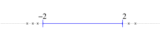
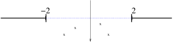
Figure 1. The meromorphic continuation

Quantum resonances are basic objects in quantum theory. They have been the focus of vast number of studies both mathematical and physical (see, e.g., [43] and references therein). Our purpose here is to study the resonances of $H_{L}$ in the asymptotic regime $L\to+\infty$. As $L\to+\infty$, $H_{L}$ converges to $H$ in the strong resolvent sense. Thus, it is natural to expect that the differences in the spectral nature between the cases $V$ periodic and $V$ random should reflect into differences in the behavior of the resonances in both cases. We shall see below that this is the case. To illustrate this as simply as possible, we begin with stating three theorems, one for periodic potentials, two for random potentials, that underline these different behaviors. These results can be considered as paradigmatic for our main results presented in section 1.
The scattering theory or the closely related questions of resonances for the operator (0.1) or for closely related one-dimensional models has already been discussed in various works both in the mathematical and physical literature (see, e.g., [12, 11, 29, 26, 40, 9, 27, 4, 25, 41]). We will make more comments on the literature as we will develop our results in section 1.

0.1. When $V$ is periodic

Assume that $V$ is $p$-periodic ($p\in\mathbb{N}^{*}$) and does not vanish identically. Consider $H=-\Delta+V$ and let $\Sigma_{\mathbb{Z}}$ be its spectrum, $\overset{\circ}{\Sigma}_{\mathbb{Z}}$ be its interior and $E\mapsto N(E)$ be its integrated density of states, i.e., the number of states of the system per unit of volume below energy $E$ (see section 1.2 and, e.g., [39] for precise definitions and details).

Theorem 0.1.

There exist

• $\mathcal{D}$, a discrete (possibly empty) set of energies in $(-2,2)\cap\overset{\circ}{\Sigma}_{\mathbb{Z}}$,

• a function $h$ that is real analytic in a complex neighborhood of $(-2,2)$ and that does vanish on $(-2,2)\setminus\mathcal{D}$

such that, for $I\subset(-2,2)\setminus\mathcal{D}$, a compact interval such that either $I\cap\Sigma_{\mathbb{Z}}=\emptyset$ or $I\subset\overset{\circ}{\Sigma}_{\mathbb{Z}}$, there exists $c_{0}>0$ such that for $L$ sufficiently large s.t. $2L\in p\mathbb{N}$, one has

• if $I\cap\Sigma_{\mathbb{Z}}=\emptyset$, then $H_{L}$ has no resonance in $I+i[-c_{0},0]$

• if $I\subset\overset{\circ}{\Sigma}_{\mathbb{Z}}$, one has

  • there are plenty of resonances in $I+i[-c_{0},0]$ ; more precisely,

    (0.2) $$\frac{\#\{z\in I+i[-c_{0},0],\ z\text{ resonance of }H_{L}\}}{2L}=\int_{I}dN(E)+o(1)$$

    where $o(1)\to 0$ as $L\to+\infty$;

  • let $(z_{j})_{j}$ the resonances of $H_{L}$ in $I+i[-c_{0},0]$ ordered by increasing real part; then,

    (0.3) $$L\cdot\text{Re}\,(z_{j+1}-z_{j})\asymp 1\quad\text{ and }\quad L\cdot\text{Im}\,z_{j}=h(\text{Re}\,z_{j})+o(1),$$

    the estimates in (0.3) being uniform for all the resonances in $I+i[-c_{0},0]$ when $L\to+\infty$.

After rescaling their width by $L$, resonances are nicely inter-spaced points lying on an analytic curve (see Fig. 2). We give a more precise description of the resonances in Theorem 1.3 and Propositions 1.1 and 1.2. In particular, we describe the set of energies $\mathcal{D}$ and the resonances near these energies: they lie further away from the real axis, the maximal distance being of order $L^{-1}\log L$ (see Fig. 3). Theorem 0.1 only describes the resonances closest to the real axis. In section 1.2, we also give results on the resonances located deeper into the lower half of the complex plane.

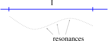
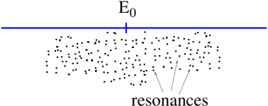
Figure 2. The rescaled resonances for the periodic (left part) and the random (right part) potential

0.2. When $V$ is random

Assume now that $V=V_{\omega}$ is the Anderson potential, i.e., its entries are i.i.d. distributed uniformly on $[0,1]$ to fix ideas. Consider $H=-\Delta+V_{\omega}$. Let $\Sigma$ be its almost sure spectrum (see, e.g., [33]), $E\mapsto n(E)$, its density of states (i.e. the derivative of the integrated density of states, see section 1.2 and, e.g., [33]) and $E\mapsto\rho(E)$, its Lyapunov exponent (see section 1.3 and, e.g., [33]). The Lyapunov exponent is known to be continuous and positive (see, e.g., [5]); the density of states satisfies $n(E)>0$ for a.e. $E\in\Sigma$ (see, e.g., [5]).
Define $H_{\omega,L}:=-\Delta+V_{\omega}\mathbf{1}_{\llbracket-L+1,L\rrbracket}$. We prove

Theorem 0.2.

Pick $I\subset(-2,2)$, a compact interval. Then,

• if $I\cap\Sigma=\emptyset$ then, there exists $c_{I}>0$ such that, $\omega$-a.s., for $L$ sufficiently large,

  $$\left\{z\text{ resonance of }H_{\omega,L}\text{ in }I+i\left(-c_{I},0\right]\right\}=\emptyset;$$

• if $I\subset\overset{\circ}{\Sigma}$ then, for any $c>0$, $\omega$-a.s., one has

  $$\lim_{L\to+\infty}\frac{1}{L}\#\left\{z\text{ resonance of }H_{\omega,L}\text{ in }I+i\left(-\infty,-e^{-cL}\right]\right\}=\int_{I}\min\left(\frac{c}{\rho(E)},1\right)n(E)dE.$$

As the first statement of Theorem 0.2 is clear, let us discuss the second. Define $\displaystyle c_{+}:=\max_{E\in I}\rho(E)$. For $c\geq c_{+}$, $\omega$-a.s., for $L$ large, the number of resonances in the strip $\{\text{Re}\,z\in I,\ \text{Im}\,z\leq-e^{-cL}\}$ is approximately $\displaystyle L\int_{I}n(E)dE$; thus, in $\{\text{Re}\,z\in I,\ -e^{c_{+}L}\leq\text{Im}\,z<0\}$, one finds at most $o(L)$ resonances. We shall see that, for $\delta>0$, $\omega$-a.s., for $L$ large, the strip $\{\text{Re}\,z\in I,\ -e^{(c_{+}+\delta)L}\leq\text{Im}\,z<0\}$ actually contains no resonance (see Theorem 1.6).
Define $\displaystyle c_{-}:=\min_{E\in I}\rho(E)$. For $c\leq c_{-}$, $\omega$-a.s., for $L$ large, the strip $\{\text{Re}\,z\in I,\ \text{Im}\,z\leq-e^{-cL}\}$ contains approximately $\displaystyle c\,L\int_{I}\frac{n(E)}{\rho(E)}dE$ resonances. We shall see that, for $\kappa\in[0,1)$, the number of resonances in the strip $\{\text{Re}\,z\in I,\ \text{Im}\,z\leq-e^{-L^{\kappa}}\}$ is $O(L^{\kappa})$, thus, $o(L)$ (cf. Theorem 1.10).
One can also describe the resonances locally. Therefore, fix $E_{0}\in(-2,2)\cap\overset{\circ}{\Sigma}$ such that $n(E_{0})>0$. Let $(z_{l}^{L}(\omega))_{l}$ be the resonances of $H_{\omega,L}$. We first rescale them. Define

(0.4) $$x_{l}^{L}(\omega)=2n(E_{0})\,L(\text{Re}\,z_{l}^{L}(\omega)-E_{0})\quad\text{and}\quad y_{l}^{L}(\omega)=-\frac{1}{L\rho(E_{0})}\log|\text{Im}\,z_{l}^{L}(\omega)|.$$

Consider now the two-dimensional point process

$$\xi_{L}(E_{0},\omega)=\sum_{z_{l}^{L}\text{ resonances of }H_{\omega,L}}\delta_{(x_{l}^{L}(\omega),y_{l}^{L}(\omega))}.$$

We prove

Theorem 0.3.

The point process $\xi_{L}$ converges weakly to a Poisson process of intensity $1$ in $\mathbb{R}\times[0,1]$.

In the random case, the structure of the (properly rescaled) resonances is quite different from that in the periodic case (see Fig. 2). The real parts of the resonances are scaled in such a way that that their average spacing becomes of order one. By Theorem 0.2, the imaginary parts are typically exponentially small (in $L$); when the resonances are rescaled as in (0.4), their imaginary parts are rewritten on a logarithmic scale so as to become of order $1$ too. Once rescaled in this way, the local picture of the resonances of $H_{\omega,L}$ is that of a two-dimensional cloud of Poisson points (see the right hand side of fig. 2).
Theorem 0.3 is the analogue for resonances of the well known result on the distribution of eigenvalues and localization centers for the Anderson model in the localized phase (see, e.g., [31, 17, 13]).
As in the case of the periodic potential, Theorem 0.3 only describes the resonances closest to the real axis. In section 1.3, we also give results on resonances located deeper into the lower half of the complex plane. Up to distances of order $L^{-\infty}$ to the real axis, the cloud of resonances (once properly rescaled) will have the same Poissonian behavior as described above (see Theorem 1.4). Besides proving Theorems 0.1 and 0.3, the goal of the paper is to describe the statistical properties of the resonances and relate them (the distribution of the resonances, the distribution of the widths) to the spectral characteristics of $H=-\Delta+V$, possibly to the distribution of its eigenvalues (see, e.g., [14]). As they can be analyzed in a very similar way, we will discuss three models:

• the model $H_{L}$ defined above,

• its analogue on the half-line $\mathbb{N}$, i.e., on $H_{L}$, we impose an additional Dirichlet boundary condition at $0$,

• the “half-infinite” model on $\ell^{2}(\mathbb{Z})$, that is,

  (0.5) $$H^{\infty}=-\Delta+W\text{ where }\begin{cases}W(n)=0\text{ for }n\geq 0\\ W(n)=V(n)\text{ for }n\leq-1\end{cases}$$

  where $V$ is chosen as above, periodic or random.

Though in the present paper we restrict ourselves to discrete models, it is clear that continuous one-dimensional models can be dealt with essentially using the methods developed in the present paper.

1. The main results

We now turn to our main results, a number of which were announced in [23]. Pick $V:\mathbb{Z}\to\mathbb{R}$ a bounded potential and, for $L\in\mathbb{N}$, consider the following operators:

• $H^{\mathbb{Z}}_{L}=-\Delta+V\mathbf{1}_{\llbracket 0,L\rrbracket}$ on $\ell^{2}(\mathbb{Z})$;

• $H^{\mathbb{N}}_{L}=-\Delta+V\mathbf{1}_{\llbracket 0,L\rrbracket}$ on $\ell^{2}(\mathbb{N})$ with Dirichlet boundary conditions at $0$;

• $H^{\infty}$ defined in (0.5).

Remark 1.1.

Here, with “Dirichlet boundary condition at $0$”, we mean that $H^{\mathbb{N}}_{L}$ is the operator $H^{\mathbb{Z}}_{L}$ restricted to the subspace $\ell^{2}(\mathbb{N})$, i.e., if $\Pi:\ell^{2}(\mathbb{Z})\to\ell^{2}(\mathbb{N})$ is the orthogonal projector on $\ell^{2}(\mathbb{N})$, one has $H^{\mathbb{N}}_{L}=\Pi H^{\mathbb{Z}}_{L}\Pi$. In the literature, this is sometime called “Dirichlet boundary condition at $-1$” (see, e.g., [39]).
For the sake of simplicity, in the half line case, we only consider Dirichlet boundary conditions at $0$. But the proofs show that these are not crucial; any self-adjoint boundary condition at $0$ would do and, mutandi mutandis, the results would be the same.
Note also that, by a shift of the potential $V$, replacing $L$ by $L+L^{\prime}$, we see that studying $H^{\mathbb{Z}}_{L}$ is equivalent to studying $H_{L,L^{\prime}}=-\Delta+V\mathbf{1}_{\llbracket-L^{\prime},L\rrbracket}$ on $\ell^{2}(\mathbb{Z})$. Thus, to derive the results of section  ‣ 0. Introduction from those in the present section, it suffices to consider the models above, in particular, $H_{L}^{\mathbb{Z}}$.

For the models $H^{\mathbb{N}}_{L}$ and $H^{\mathbb{Z}}_{L}$, we start with a discussion of the existence of a meromorphic continuation of the resolvent, then, study the resonances when $V$ is periodic and finally turn to the case when $V$ is random.
As $H^{\infty}$ is not a relatively compact perturbation of the Laplacian, the existence of a meromorphic continuation of its resolvent depends on the nature of $V$; so, it will be discussed when specializing to $V$ periodic or random.

Remark 1.2 (Notations).

In the sequel, we write $a\lesssim b$ if for some $C>0$ (independent of the parameters coming into $a$ or $b$), one has $a\leq Cb$. We write $a\asymp b$ if $a\lesssim b$ and $b\lesssim a$.

1.1. The meromorphic continuation of the resolvent

One proves the well known and simple

Theorem 1.1.

The operator valued functions $z\in\mathbb{C}^{+}\mapsto(z-H^{\mathbb{N}}_{L})^{-1}$ and $z\in\mathbb{C}^{+}\mapsto(z-H^{\mathbb{Z}}_{L})^{-1}$) admit a meromorphic continuation from $\mathbb{C}^{+}$ to $\displaystyle\mathbb{C}\setminus\left((-\infty,-2]\cup[2,+\infty)\right)$ through $(-2,2)$ (see Fig. 1) with values in the operators from $l^{2}_{\text{comp}}$ to $l^{2}_{\text{loc}}$.
Moreover, the number of poles of each of these meromorphic continuations in the lower half-plane is at most equal to $L$.

The resonances are defined to be the poles of this meromorphic continuation (see Fig. 1).

1.2. The periodic case

We assume that, for some $p>0$, one has

(1.1) $$V_{n+p}=V_{n}\quad\text{for all}\quad n\geq 0.$$

Let $\Sigma_{\mathbb{N}}$ be the spectrum of $H^{\mathbb{N}}=-\Delta+V$ acting on $\ell^{2}(\mathbb{N})$ with Dirichlet boundary condition at $0$ and $\Sigma_{\mathbb{Z}}$ be the spectrum of $H^{\mathbb{Z}}=-\Delta+V$ acting on $\ell^{2}(\mathbb{Z})$. One has the following description for these spectra:

• $\Sigma_{\mathbb{Z}}$ is a union of intervals, i.e., $\displaystyle\Sigma_{\mathbb{Z}}:=\sigma(H)=\bigcup_{j=1}^{p}[E_{j}^{-},E_{j}^{+}]$ where $E_{j}^{-}<E_{j}^{+}$ ($1\leq j\leq p$) and $a^{+}_{j-1}\leq E_{j}^{-}$ ($2\leq j\leq p$) (see , e.g., [42]); the spectrum of $H^{\mathbb{Z}}$ is purely absolutely continuous and the spectral resolution can be obtained via a Bloch-Floquet decomposition (see, e.g., [42]);

• on $\ell^{2}(\mathbb{N})$ (see, e.g., [34]), one has

  • $\Sigma_{\mathbb{N}}=\Sigma_{\mathbb{Z}}\cup\{v_{j};1\leq j\leq n\}$ and $\Sigma_{\mathbb{Z}}$ is the a.c. spectrum of $H$;

  • the $(v_{j})_{0\leq j\leq n}$ are isolated simple eigenvalues associated to exponentially decaying eigenfunctions.

It may happen that some of the gaps are closed, i.e., that the number of connected components of $\Sigma_{\mathbb{Z}}$ be strictly less than $p$. There still is a natural way to write $\displaystyle\Sigma_{\mathbb{Z}}:=\sigma(H)=\bigcup_{j=1}^{p}[E_{j}^{-},E_{j}^{+}]$ (see section 4.1.1), but in this case, for some $j$’s, one has $E_{j-1}^{+}=E_{j}^{-}$; the energies $E_{j-1}^{+}=E_{j}^{-}$, we shall call closed gaps (see Definition 4.1). The existence of closed gaps is non generic (see [42]).
The operators $H^{\bullet}$ (for $\bullet\in\{\mathbb{N},\mathbb{Z}\}$) admit an integrated density of states defined by

(1.2) $$N(E)=\lim_{L\to+\infty}\frac{\#\{\text{eigenvalues of }(-\Delta+V)_{|\llbracket-L,L\rrbracket\cap\bullet}\text{ in }(-\infty,E]\}}{\#(\llbracket-L,L\rrbracket\cap\bullet)}.$$

Here, the restriction of $-\Delta+V$ to $\llbracket-L,L\rrbracket\cap\bullet$ is taken with Dirichlet boundary conditions; this is to fix ideas as it is known that, in the limit $L\to+\infty$, other self-adjoint boundary conditions would yield the same result for the limit (1.2).
The integrated density of states is the same for $H^{\mathbb{N}}$ and $H^{\mathbb{Z}}$ (see, e.g., [33]). It defines the distribution function of some probability measure on $\Sigma_{\mathbb{Z}}$ that is real analytic on $\overset{\circ}{\Sigma}_{\mathbb{Z}}$. Let $n$ denote the density of states of $H^{\mathbb{N}}$ and $H^{\mathbb{Z}}$, that is, $\displaystyle n(E)=\frac{dN}{dE}(E)$.

Remark 1.3.

When $L$ gets large, as $H^{\mathbb{N}}_{L}$ tends to $H^{\mathbb{N}}$ in strong resolvent sense, interesting phenomena for the resonances of $H_{L}^{\mathbb{N}}$ should take place near energies in $\Sigma_{\mathbb{N}}$.
Define $\tau_{k}$ to be the shift by $k$ steps to the left, that is, $\tau_{k}V(\cdot)=V(\cdot+k)$. Then, for $(\ell_{L})_{L}$ s.t. $l_{L}\to+\infty$ and $L-\ell_{L}\to+\infty$ when $L\to+\infty$, $\tau^{*}_{l_{L}}H^{\mathbb{Z}}_{L}\tau_{l_{L}}$ tend to $H^{\mathbb{Z}}$ in strong resolvent sense. Thus, interesting phenomena for the resonances of $H_{L}^{\mathbb{Z}}$ should take place near energies in $\Sigma_{\mathbb{Z}}$.

1.2.1. Resonance free regions

We start with a description of resonance free regions near the real axis. Therefore, we introduce some operators on the positive and the negative half-lattice.
Above we have defined $H_{\mathbb{N}}$; we shall need another auxiliary operator. On $\ell^{2}(\mathbb{Z}_{-})$ (where $\mathbb{Z}_{-}=\{n\leq 0\}$), consider the operator $H_{k}^{-}=-\Delta+\tau_{k}V$ with Dirichlet boundary condition at $0$ (where $\tau_{k}$ is defined to be the shift by $k$ steps to the left, that is, $\tau_{k}V(\cdot)=V(\cdot+k)$). Let $\Sigma_{k}^{-}=\sigma(H^{-}_{k})$.
As is the case for $H^{\mathbb{N}}$, one knows that $\sigma_{\text{ess}}(H^{-}_{k})=\Sigma_{\mathbb{Z}}$ and that $\sigma_{\text{ess}}(H^{-}_{k})$ is purely absolutely continuous (see, e.g., [39, Chapter 7]). $H^{-}_{k}$ may also have discrete eigenvalues in $\mathbb{R}\setminus\Sigma_{\mathbb{Z}}$.
We prove

Theorem 1.2.

Let $I$ be a compact interval in $(-2,2)$. Then,

1. if $I\subset\mathbb{R}\setminus\Sigma_{\mathbb{N}}$ (resp. $I\subset\mathbb{R}\setminus\Sigma_{\mathbb{Z}}$), then, there exists $c>0$ such that, for $L$ sufficiently large, $H^{\mathbb{N}}_{L}$ (resp. $H^{\mathbb{Z}}_{L}$) has no resonances in the rectangle $\{\text{Re}\,z\in I,\ \text{Im}\,z\in[-c,0]\}$;

2. if $I\subset\Sigma_{\mathbb{Z}}$, then, there exists $c>0$ such that, for $L$ sufficiently large, $H^{\mathbb{N}}_{L}$ and $H^{\mathbb{Z}}_{L}$ have no resonances in the rectangle $\{\text{Re}\,z\in I,\ \text{Im}\,z\in[-c/L,0]\}$;

3. fix $0\leq k\leq p-1$ and assume the compact interval $I$ to be such that $\{v_{j}\}=\overset{\circ}{I}\cap\Sigma_{\mathbb{N}}=I\cap\Sigma_{\mathbb{N}}$ and $I\cap\Sigma_{\mathbb{Z}}=\emptyset$ ($(v_{j})_{j}$ are defined in the beginning of section 1.2):

   1. if $I\cap\Sigma^{-}_{k}=\emptyset$ then, there exists $c>0$ such that, for $L$ sufficiently large such that $L\equiv k\mod p$, $H^{\mathbb{N}}_{L}$ has a unique resonance in the rectangle $\{\text{Re}\,z\in I,\ -c\leq\text{Im}\,z\leq 0\}$; moreover, this resonance, say $z_{j}$, is simple and satisfies $\text{Im}\,z_{j}\asymp-e^{-\rho_{j}L}$ and $|z_{j}-\lambda_{j}|\asymp e^{-\rho_{j}L}$ for some $\rho_{j}>0$ independent of $L$;

   2. if $I\cap\Sigma^{-}_{k}\not=\emptyset$ then, there exists $c>0$ such that, for $L$ sufficiently large such that $L\equiv k\mod p$, $H^{\mathbb{N}}_{L}$ has no resonance in the rectangle $\{\text{Re}\,z\in I,\ -c\leq\text{Im}\,z\leq 0\}$.

So, below the spectral interval $(-2,2)$, there exists a resonance free region of width at least of order $L^{-1}$. For $H^{\mathbb{N}}_{L}$, if $L\equiv k\mod p$, each discrete eigenvalue of $H^{\mathbb{N}}$ that is not an eigenvalue of $H^{-}_{k}$ generates a resonance for $H^{\mathbb{N}}_{L}$ exponentially close to the real axis (when $L$ is large). When the eigenvalue of $H_{k}^{-}$ is also an eigenvalue of $H^{\mathbb{N}}=H_{0}^{+}$, it may also generate a resonance but only much further away in the complex plane, at least at a distance of order $1$ to the real axis.
In case (3)(a) of Theorem 1.2, one can give an asymptotic expansion for the resonances (see section 5.2.1).
We now turn to the description of the resonances of $H^{\bullet}_{L}$ near $[-2,2]$. Therefore, it will be useful to introduce a number of auxiliary functions and operators.

1.2.2. Some auxiliary functions

To $H_{k}^{-}$ defined above, we associate $N^{-}_{k}$, the distribution function of its spectral measure (that is a probability measure), i.e., for $\varphi\in{\mathcal{C}}_{0}^{\infty}(\mathbb{R})$, we define $\displaystyle\int_{\mathbb{R}}\varphi(\lambda)dN^{-}_{k}(\lambda):=\varphi(H_{k}^{-})(0,0)$ where $(\varphi(H_{k}^{-})(x,y))_{(x,y)\in(\mathbb{Z}_{-})^{2}}$ denotes the kernel of the operator $\varphi(H_{k}^{-})$.
On $\overset{\circ}{\Sigma}_{\mathbb{Z}}$, the spectral measure $dN_{k}^{-}$ admits a density with respect to the Lebesgue measure, say, $n^{-}_{k}$, and this density is real analytic (see Proposition 5.1).
For $E\in\overset{\circ}{\Sigma}_{\mathbb{Z}}$, define

(1.3) $$S^{-}_{k}(E):=\text{p.v.}\left(\int_{\mathbb{R}}\frac{dN^{-}_{k}(\lambda)}{\lambda-E}\right)=\lim_{\varepsilon\downarrow 0}\left(\int_{-\infty}^{E-\varepsilon}\frac{dN^{-}_{k}(\lambda)}{\lambda-E}-\int_{E+\varepsilon}^{+\infty}\frac{dN^{-}_{k}(\lambda)}{\lambda-E}\right).$$

The existence and analyticity of the Cauchy principal value $S^{-}_{k}$ on $\overset{\circ}{\Sigma}_{\mathbb{Z}}$ is guaranteed by the analyticity of $n^{-}_{k}$ (see, e.g., [18]). Moreover, for $E\in\overset{\circ}{\Sigma}_{\mathbb{Z}}$, one has

(1.4) $$S^{-}_{k}(E)=\lim_{\varepsilon\to 0^{+}}\int_{\mathbb{R}}\frac{dN^{-}_{k}(\lambda)}{\lambda-E-i\varepsilon}-i\pi n_{k}^{-}(E).$$

In the lower half-plane $\{$Im$\,E<0\}$, define the function

(1.5) $$\Xi^{-}_{k}(E):=\int_{\mathbb{R}}\frac{dN_{k}^{-}(\lambda)}{\lambda-E}+e^{-i\arccos(E/2)}=\int_{\mathbb{R}}\frac{dN_{k}^{-}(\lambda)}{\lambda-E}+E/2+\sqrt{(E/2)^{2}-1}$$

where

• in the first formula, the function $z\mapsto\arccos z$ is the analytic continuation to the lower half-plane of the determination taking values in $[-\pi,0]$ on the interval $[-1,1]$;

• in the second formula, the branch of the square root $z\mapsto\sqrt{z^{2}-1}$ has positive imaginary part for $z\in(-1,1)$.

The function $\Xi^{-}_{k}$ is analytic in $\{$Im$\,E<0\}$ and in a neighborhood of $(-2,2)\cap\overset{\circ}{\Sigma}_{\mathbb{Z}}$. Moreover, $\Xi^{-}_{k}$ vanishes identically if and only if $V\equiv 0$ (see Proposition 5.2).
From now on we assume that $V\not\equiv 0$. In this case, in $\{$Im$\,E<0\}$ and on $(-2,2)\cap\overset{\circ}{\Sigma}_{\mathbb{Z}}$, the analytic function $\Xi_{k}^{-}$ has only finitely many zeros, each of finite multiplicity (see Proposition 5.2).
We shall need the analogues of the above defined functions the already introduced operator $H_{0}^{+}:=H^{\mathbb{N}}=-\Delta+V$ considered on $\ell^{2}(\mathbb{N})$ with Dirichlet boundary conditions at $0$. We define the function $N^{+}_{0}$ as the distribution function of the spectral measure of $H_{0}^{+}$, i.e., for $\varphi\in{\mathcal{C}}_{0}^{\infty}(\mathbb{R})$, we define $\displaystyle\int_{\mathbb{R}}\varphi(\lambda)dN^{+}_{0}(\lambda):=\varphi(H_{0}^{+})(0,0)$. In the same way as we have defined $n_{k}^{-}$, $S_{k}^{-}$ and $\Xi_{k}^{-}$ from $H_{k}^{-}$, one can define $n_{0}^{+}$, $S_{0}^{+}$ and $\Xi_{0}^{+}$ from $H_{0}^{+}$. They also satisfy Proposition 5.1, relation (1.4) and Proposition 5.2.
For the description of the resonances, it will be convenient to define the following functions on $\overset{\circ}{\Sigma}_{\mathbb{Z}}$

(1.6) $$c^{\mathbb{N}}(E):=i+\frac{\Xi_{k}^{-}(E)}{\pi\,n_{k}^{-}(E)}=\frac{1}{\pi\,n_{k}^{-}(E)}\left(S_{k}^{-}(E)+e^{-i\arccos(E/2)}\right)$$

and

(1.7) $$c^{\mathbb{Z}}(E):=\frac{\displaystyle\frac{\left(S^{+}_{0}(E)+e^{-i\arccos(E/2)}\right)\left(S_{k}^{-}(E)+e^{-i\arccos(E/2)}\right)}{n_{0}^{+}(E)\,n_{k}^{-}(E)}-\pi^{2}}{\displaystyle\frac{\pi\left(S^{+}_{0}(E)+e^{-i\arccos(E/2)}\right)}{n_{0}^{+}(E)}+\frac{\pi\left(S_{k}^{-}(E)+e^{-i\arccos(E/2)}\right)}{n_{k}^{-}(E)}}.$$

We shall see that the the zeros of $c^{\bullet}-i$ play a special role for the resonances of $H^{\bullet}_{L}$: therefore, we define

(1.8) $$\mathcal{D}^{\bullet}=\left\{z\in\overset{\circ}{\Sigma}_{\mathbb{Z}};\ c^{\bullet}(z)=i\right\}$$

The set $\mathcal{D}$ introduced in Theorem 0.1 is the set $\mathcal{D}^{\mathbb{Z}}\cap(-2,2)$.

Remark 1.4.

Before describing the resonances, let us explain why the operators $H_{0}^{+}$ and $H_{k}^{-}$ naturally occur in this study. They respectrively are the strong resolvent limits (when $L\to+\infty$ s.t. $L\in p\mathbb{N}+k$) of the operator $H^{\mathbb{Z}}_{L}$ restricted to $\llbracket 0,L\rrbracket$ with Dirichlet boundary conditions at $0$ and $L$ “seen” respectively from the left and the right hand side.
Indeed, define $H_{L}$ to be the operator $H^{\mathbb{N}}_{L}$ restricted to $\llbracket 0,L\rrbracket$ with Dirichlet boundary conditions at $L$ (see Remark 1.1). Note that $H_{L}$ is also the operator $H^{\mathbb{Z}}_{L}$ restricted to $\llbracket 0,L\rrbracket$ with Dirichlet boundary conditions at $0$ and $L$.
Clearly, the operator $H_{0}^{+}$ is the strong resolvent limit of $H_{L}$ when $L\to+\infty$.
If $\tilde{\tau}_{L}$ denotes the translation by $-L$ that unitarily maps $\ell^{2}(\llbracket 0,L\rrbracket)$ into $\ell^{2}(\llbracket-L,0\rrbracket)$, then, $\tilde{H}_{L}=\tilde{\tau}_{L}H_{L}\tilde{\tau}^{*}_{L}$ converges in the strong resolvent sense to $H_{k}^{-}$ when $L\to+\infty$ and $L\equiv k\mod(p)$. Indeed, $\tau_{L}V=\tau_{k}V$ as $V$ is $p$ periodic.

1.2.3. Description of the resonances closest to the real axis

Let $(\lambda_{l})_{0\leq l\leq L}=(\lambda_{l}^{L})_{0\leq l\leq L}$ be the eigenvalues of $H_{L}$ (that is, the eigenvalues of $H^{\mathbb{N}}_{L}$ or $H^{\mathbb{Z}}_{L}$ restricted to $\llbracket 0,L\rrbracket$ with Dirichlet boundary conditions, see remark 1.1) listed in increasing order. They are described in Theorem 4.2; those away from the edges of $\Sigma_{\mathbb{Z}}$ are shown to be nicely interspaced points at a distance roughly $L^{-1}$ from one another.
We first state our most general result describing the resonances in a uniform way. We, then, derive two corollaries describing the behavior of the resonance, first, far from the set of exceptional energies $\mathcal{D}^{\bullet}$, second, close to an exceptional energy.
Pick a compact interval $I\subset(-2,2)\cap\overset{\circ}{\Sigma}_{\mathbb{Z}}$. For $\bullet\in\{\mathbb{N},\mathbb{Z}\}$ and $\lambda_{l}\in I$, for $L$ large, define the complex number

(1.9) $$\tilde{z}^{\bullet}_{l}=\lambda_{l}+\frac{1}{\pi\,n(\lambda_{l})\,L}\cot^{-1}\circ\,c^{\bullet}\left[\lambda_{l}+\frac{1}{\pi\,n(\lambda_{l})\,L}\cot^{-1}\circ\,c^{\bullet}\left(\lambda_{l}-i\frac{\log L}{L}\right)\right]$$

where the determination of $\cot^{-1}$ is the inverse of the determination $z\mapsto\cot(z)$ mapping $\left[0,\pi\right)\times(0,-\infty)$ onto $\mathbb{C}^{+}\setminus\{i\}$.
Note that, by Proposition 5.3, for $L$ sufficiently large, we know that, for any $l$ such that $\lambda_{l}\in I$, one has

$$\text{Im}\,c^{\bullet}\left(\lambda_{l}-i\frac{\log L}{L}\right)\in(0,+\infty)\setminus\{1\}$$

and

$$\text{Im}\,c^{\bullet}\left[\lambda_{l}+\frac{1}{\pi\,n(\lambda_{l})\,L}\cot^{-1}\circ\,c^{\bullet}\left(\lambda_{l}-i\frac{\log L}{L}\right)\right]\in(0,+\infty)\setminus\{1\}.$$

Thus, the formula (1.9) defines $\tilde{z}^{\bullet}_{l}$ properly and in a unique way. Moreover, as the zeros of $E\mapsto c^{\bullet}(E)-i$ are of finite order, one checks that

(1.10) $$-\log L\lesssim\,L\cdot\text{Im}\,\tilde{z}^{\bullet}_{l}\lesssim-1\quad\text{ and }\quad 1\lesssim L\cdot\text{Re}\,\left(\tilde{z}^{\bullet}_{l+1}-\tilde{z}^{\bullet}_{l}\right)$$

where the constants are uniform for $l$ such that $\lambda_{l}\in I$.
We prove the

Theorem 1.3.

Pick $\bullet\in\{\mathbb{N},\mathbb{Z}\}$ and $k\in\{0,\cdots,p-1\}$. Let $E_{0}\in(-2,2)\cap\overset{\circ}{\Sigma}_{\mathbb{Z}}$.
Then, there exists $\eta_{0}>0$ and $L_{0}>0$ such that, for $L>L_{0}$ satisfying $L=k\mod(p)$, for each $\lambda_{l}\in I:=[E_{0}-\eta_{0},E_{0}+\eta_{0}]$, there exists a unique resonance of $H^{\bullet}_{L}$, say $z^{\bullet}_{l}$, in the rectangle

$$\left[\frac{\text{Re}\,(\tilde{z}^{\bullet}_{l}+\tilde{z}^{\bullet}_{l-1})}{2},\frac{\text{Re}\,(\tilde{z}^{\bullet}_{l}+\tilde{z}^{\bullet}_{l+1})}{2}\right]+i\left[-\eta_{0},0\right];$$

this resonance is simple and it satisfies $\displaystyle\left|z^{\bullet}_{l}-\tilde{z}^{\bullet}_{l}\right|\lesssim\frac{1}{L\log L}$.

This result calls for a few comments. First, the picture one gets for the resonances can be described as follows (see also Figure 3). As long as $\lambda_{l}$ stays away from any zero of $E\mapsto c^{\bullet}(E)-i$, the resonances are nicely spaced points as the following proposition proves.

Proposition 1.1.

Pick $\bullet\in\{\mathbb{N},\mathbb{Z}\}$ and $k\in\{0,\cdots,p-1\}$. Let $I\subset(-2,2)\cap\overset{\circ}{\Sigma}_{\mathbb{Z}}$ be a compact interval such that $I\cap\mathcal{D}^{\bullet}=\emptyset$.
Then, for $L$ sufficiently large, for each $\lambda_{l}\in I$, the resonance $z^{\bullet}_{l}$ admits a complete asymptotic expansion in powers of $L^{-1}$ and one has

(1.11) $$z^{\bullet}_{l}=\lambda_{l}+\frac{1}{\pi\,n(\lambda_{l})\,L}\cot^{-1}\circ\,c^{\bullet}(\lambda_{l})+O\left(\frac{1}{L^{2}}\right)$$

where the remainder term is uniform in $l$.

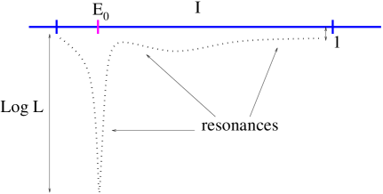
Figure 3. The resonances close to the real axis in the periodic case (after rescaling their imaginary parts by $L$)

The proof of Proposition 1.1 actually yields a complete asymptotic expansion in powers of $L^{-1}$ for the resonances in this zone (see section 5.2.5).
Proposition 1.1 implies Theorem 0.1: we chose $\bullet=\mathbb{Z}$, $k=0$ and the set $\mathcal{D}$ of exceptional points in Theorem 0.1 is exactly $\mathcal{D}^{\mathbb{Z}}\cap(-2,2)$; to obtain (0.3), it suffices to use the asymptotic form of the Dirichlet eigenvalues given by Theorem 4.2.
Near the zeros of $E\mapsto c^{\bullet}(E)-i$, the resonances take a “plunge” into the lower half of the complex plane (see Figure 3) and their imaginary part becomes of order $L^{-1}\log L$. Indeed, Theorem 1.3 and (1.9) imply

Proposition 1.2.

Pick $\bullet\in\{\mathbb{N},\mathbb{Z}\}$ and $k\in\{0,\cdots,p-1\}$. Let $E_{0}\in\mathcal{D}^{\bullet}$ be a zero of $E\mapsto c^{\bullet}(E)-i$ of order $q$ in $(-2,2)\cap\overset{\circ}{\Sigma}_{\mathbb{Z}}$.
Then, for $\alpha>0$, for $L$ sufficiently large, if $l$ is such that $|\lambda_{l}-E_{0}|\leq L^{-\alpha}$, the resonance $z^{\bullet}_{l}$ satisfies

(1.12) $$\text{Im}\,z^{\bullet}_{l}=\frac{q}{2\pi\,n(\lambda_{l})}\cdot\frac{\log\left(|\lambda_{l}-E_{0}|^{2}+\left(\frac{q\,\log L}{2\pi\,n(\lambda_{l})\,L}\right)^{2}\right)}{2\,L}\cdot(1+o(1))$$

where the remainder term is uniform in $l$ such that $|\lambda_{l}-E_{0}|\leq L^{-\alpha}$.

When $\bullet=\mathbb{Z}$, the asymptotic (1.12) shows that there can be a “resonance” phenomenon for resonances: when the two functions $\Xi_{k}^{-}$ and $\Xi_{0}^{+}$ share a zero at the same real energy, the maximal width of the resonances increases; indeed, the factor in front of $L^{-1}\log L$ is proportional to the multiplicity of the zero of $\Xi_{k}^{-}\,\Xi_{0}^{+}$.

1.2.4. Description of the low lying resonances

The resonances found in Theorem 1.3 are not necessarily the only ones: deeper into the lower complex plane, one may find more resonances. They are related to the zeros of $\Xi_{k}^{-}$ when $\bullet=\mathbb{N}$ and $\Xi_{k}^{-}\,\Xi_{0}^{+}$ when $\bullet=\mathbb{Z}$ (see Proposition 5.3).
We now study what happens below the line $\{$Im$\,z=-\eta_{0}\}$ (see Theorem 1.3) for the resonances of $H^{\mathbb{N}}_{L}$ and $H^{\mathbb{Z}}_{L}$.
The functions $\Xi_{k}^{-}$ and $\Xi_{0}^{+}$ are analytic in the lower half plane and, by Proposition 5.2, they don’t vanish in an neighborhood of $-i\infty$. Hence, the functions $\Xi_{k}^{-}$ and $\Xi_{0}^{+}$ have only finitely many zeros in the lower half plane.
We prove

Theorem 1.4.

Pick $\bullet\in\{\mathbb{N},\mathbb{Z}\}$ and $k\in\{0,\cdots,p-1\}$. Let $(E^{\bullet}_{j})_{1\leq j\leq J}$ be the zeros of $E\mapsto c^{\bullet}(E)-i$ in $I+i(-\infty,0)$. Pick $E_{0}\in(-2,2)\cap\overset{\circ}{\Sigma}_{\mathbb{Z}}$.
There exists $\eta_{0}>0$ such that, for $I=E_{0}+[-\eta_{0},\eta_{0}]$, for $L$ sufficiently large s.t. $L\equiv k\mod(p)$, one has,

• if $E_{0}\not\in\{\text{Re}\,E^{\bullet}_{j};\ 1\leq j\leq J\}$, then, in the rectangle $I+i(-\infty,0]$, the only resonances of $H^{\mathbb{N}}_{L}$ and $H^{\mathbb{Z}}_{L}$ are those given by Theorem 1.3;

• if $E_{0}\in\{\text{Re}\,E^{\bullet}_{j};\ 1\leq j\leq J\}$, then,

  • in the rectangle $I+i[-\eta_{0},0]$, the only resonances of $H^{\mathbb{N}}_{L}$ and $H^{\mathbb{Z}}_{L}$ are those given by Theorem 1.3;

  • in the strip $I+i[-\infty,-\eta_{0}]$, the resonances of $H^{\bullet}_{L}$ are contained in $\displaystyle\bigcup_{j=1}^{J}D\left(E^{\bullet}_{j},e^{-\eta_{0}L}\right)$

  • in $\displaystyle D\left(E^{\bullet}_{j},e^{-\eta_{0}L}\right)$, the number of resonances (counted with multiplicity) is equal to the order of $E^{\bullet}_{j}$ as a zero of $E\mapsto c^{\bullet}(E)-i$.

We see that the total number of resonances below a compact subset of $(-2,2)\cap\overset{\circ}{\Sigma}_{\mathbb{Z}}$ that do not tend to the real axis when $L\to+\infty$ is finite. These resonances are related to the resonances of $H^{\infty}$ to which we turn now.

1.2.5. The half-line periodic perturbation

Fix $p\in\mathbb{N}^{*}$. On $\ell^{2}(\mathbb{Z})$, we now consider the operator $H^{\infty}=-\Delta+V$ where $V(n)=0$ for $n\geq 0$ and $V(n+p)=V(n)$ for $n\leq-1$. We prove

Theorem 1.5.

The resolvent of $H^{\infty}$ can be analytically continued from the upper half-plane through $(-2,2)\cap\overset{\circ}{\Sigma}_{Z}$ to the lower half plane. The resulting operator does not have any poles in the lower half-plane or on $(-2,2)\cap\overset{\circ}{\Sigma}_{Z}$.
The resolvent of $H^{\infty}$ can be analytically continued from the upper half-plane through $(-2,2)\setminus\Sigma_{\mathbb{Z}}$ (resp. $\overset{\circ}{\Sigma}_{Z}\setminus[-2,2]$) to the lower half plane; the poles of the continuation through $(-2,2)\setminus\Sigma_{\mathbb{Z}}$ (resp. $\overset{\circ}{\Sigma}_{Z}\setminus[-2,2]$) are exactly the zeros of the function $\displaystyle E\mapsto 1-e^{i\theta(E)}\int_{\mathbb{R}}\frac{dN^{-}_{p-1}(\lambda)}{\lambda-E}$ when continued from the upper half-plane through $(-2,2)\setminus\Sigma_{\mathbb{Z}}$ (resp. $\overset{\circ}{\Sigma}_{Z}\setminus[-2,2]$) to the lower half-plane.

Remark 1.5.

In Theorem 1.5 and below, every time we consider the analytic continuation of a resolvent through some open subset of the real line, we implicitly assume the open subset to be non empty.

In figure 4, to illustrate Theorem 1.5, assuming that $\Sigma_{\mathbb{Z}}$ (in blue) has a single gap that is contained in $(-2,2)$, we drew the various analytic continuations of the resolvent of $H^{\infty}$ and the presence or absence of resonances for the different continuations .

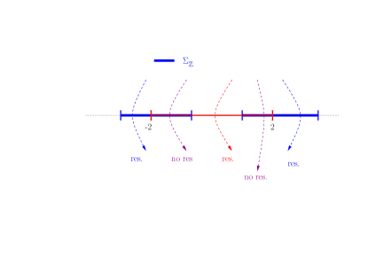
Figure 4. The analytic continuation of the resolvent and resonances for $H^{\infty}$

Using the same arguments as in the proof of Proposition 5.2, one easily sees that the continuations of the function $\displaystyle E\mapsto 1-e^{i\theta(E)}\int_{\mathbb{R}}\frac{dN^{-}_{p-1}(\lambda)}{\lambda-E}$ to the lower half plane through $(-2,2)\setminus\Sigma_{\mathbb{Z}}$ and $\overset{\circ}{\Sigma}_{Z}\setminus[-2,2]$ have at most finitely many zeros and that these zeros are away from the real axis.
This also implies that the spectrum on $H^{\infty}$ in $[-2,2]\cup\Sigma_{\mathbb{Z}}$ is purely absolutely continuous except possibly at the points of $\partial\Sigma_{\mathbb{Z}}\cup\{-2,2\}$ where $\partial\Sigma_{\mathbb{Z}}$ is the set of edges of $\Sigma_{\mathbb{Z}}$.

1.3. The random case

We now turn to the random case. Let $V=V_{\omega}$ where $(V_{\omega}(n))_{n\in\mathbb{Z}}$ are bounded independent and identically distributed random variables. Assume that the common law of the random variables admits a bounded compactly supported density, say, $g$.
Set $H^{\mathbb{N}}_{\omega}=-\Delta+V_{\omega}$ on $\ell^{2}(\mathbb{N})$ (with Dirichlet boundary condition at $0$ to fix ideas). Let $\sigma(H^{\mathbb{N}}_{\omega})$ be the spectrum of $H^{\mathbb{N}}_{\omega}$. Consider also $H^{\mathbb{Z}}_{\omega}=-\Delta+V_{\omega}$ acting on $\ell^{2}(\mathbb{Z})$. Then, one knows (see, e.g., [19]) that, $\omega$ almost surely,

(1.13) $$\sigma(H^{\mathbb{Z}}_{\omega})=\Sigma:=[-2,2]+\text{supp}\,g.$$

One has the following description for the spectra $\sigma(H^{\mathbb{N}}_{\omega})$ and $\sigma(H^{\mathbb{Z}}_{\omega})$:

• $\omega$-almost surely, $\sigma(H^{\mathbb{Z}}_{\omega})=\Sigma$; the spectrum is purely punctual; it consists of simple eigenvalues associated to exponentially decaying eigenfunctions (Anderson localization, see, e.g., [33, 19]); one can prove that, under the assumptions made above, the whole spectrum is dynamically localized (see, e.g., [10] and references therein);

• for $H^{\mathbb{N}}_{\omega}$ (see, e.g., [33, 7]), one has, $\omega$-almost surely, $\sigma(H^{\mathbb{N}}_{\omega})=\Sigma\cup K_{\omega}$ where

  • $\Sigma$ is the essential spectrum of $H^{\mathbb{N}}_{\omega}$; it consists of simple eigenvalues associated to exponentially decaying eigenfunctions;

  • the set $K_{\omega}$ is the discrete spectrum of $H^{\mathbb{N}}_{\omega}$; it may be empty and depends on $\omega$.

1.3.1. The integrated density of states and the Lyapunov exponent

It is well known (see, e.g., [33]) that the integrated density of states of $H$, say, $N(E)$ is defined as the following limit

(1.14) $$N(E)=\lim_{L\to+\infty}\frac{\#\{\text{eigenvalues of }H^{\mathbb{Z}}_{\omega|\llbracket-L,L\rrbracket}\text{ in }(-\infty,E]\}}{2L+1}.$$

The above limit does not depend on the boundary conditions used to define the restriction $H^{\mathbb{Z}}_{\omega|\llbracket-L,L\rrbracket}$. It defines the distribution function of a probability measure supported on $\Sigma$. Under our assumptions on the random potential, $N$ is known to be Lipschitz continuous ([33, 19]). Let $\displaystyle n(E)=\frac{dN}{dE}(E)$ be its derivative; it exists for almost all energies. If one assumes more regularity on $g$ the density of the random variables $(\omega_{n})_{n}$, then, the density of states $n$ can be shown to exist everywhere and to be regular (see, e.g., [10]).
One also defines the Lyapunov exponent, say $\rho(E)$ as follows

$$\rho(E):=\lim_{L\to+\infty}\frac{\log\|T_{L}(E,\omega)\|}{L+1}$$

where

(1.15) $$T_{L}(E;\omega):=\begin{pmatrix}E-V_{\omega}(L)&-1\\ 1&0\end{pmatrix}\times\cdots\times\begin{pmatrix}E-V_{\omega}(0)&-1\\ 1&0\end{pmatrix}$$

For any $E$, $\omega$-almost surely, the Lyapunov exponent is known to exist and to be independent of $\omega$ (see, e.g., [10, 33, 7]). It is positive at all energies. Moreover, by the Thouless formula [10], it is positive and continuous for all $E$ and it is the harmonic conjugate of $n(E)$.For $\bullet\in\{\mathbb{N},\mathbb{Z}\}$, we now define $H^{\bullet}_{\omega,L}$ to be the operator $-\Delta^{\bullet}+V_{\omega}\mathbf{1}_{\llbracket 0,L\rrbracket}$. The goal of the next sections is to describe the resonances of these operators in the limit $L\to+\infty$.

As in the case of a periodic potential $V$, the resonances are defined as the poles of the analytic continuation of $z\mapsto(H^{\bullet}_{\omega,L}-z)^{-1}$ from $\mathbb{C}^{+}$ through $(-2,2)$ (see Theorem 1.1).

1.3.2. Resonance free regions

We again start with a description of the resonance free region near a compact interval in $(-2,2)$. As in the periodic case, the size of the $H^{\bullet}_{\omega,L}$-resonance free region below a given energy will depend on whether this energy belongs to $\sigma(H^{\bullet}_{\omega})$ or not. We prove

Theorem 1.6.

Fix $\bullet\in\{\mathbb{N},\mathbb{Z}\}$. Let $I$ be a compact interval in $(-2,2)$. Then, $\omega$-a.s., one has

1. for $\bullet\in\{\mathbb{N},\mathbb{Z}\}$, if $I\subset\mathbb{R}\setminus\sigma(H^{\bullet}_{\omega})$, then, there exists $C>0$ such that, for $L$ sufficiently large, there are no resonances of $H^{\bullet}_{\omega,L}$ in the rectangle $\{\text{Re}\,z\in I,\ 0\geq\text{Im}\,z\geq-1/C\}$;

2. if $I\subset\overset{\circ}{\Sigma}$, then, for $\varepsilon\in(0,1)$, there exists $L_{0}>0$ such that, for $L\geq L_{0}$, there are no resonances of $H^{\bullet}_{\omega,L}$ in the rectangle $\{\text{Re}\,z\in I,\ 0\geq\text{Im}\,z\geq-e^{-2\eta_{\bullet}\rho L(1+\varepsilon)})\}$ where

   • $\rho$ is the maximum of the Lyapunov exponent $\rho(E)$ on $I$

   • $\displaystyle\eta_{\bullet}=\begin{cases}1\text{ if }\bullet=\mathbb{N},\\ 1/2\text{ if }\bullet=\mathbb{Z}.\end{cases}$

3. pick $v_{j}=v_{j}(\omega)\in K_{\omega}$ (see the description of the spectrum of $H_{\omega}^{\mathbb{N}}$ just above section 1.3.1) and assume that $\{v_{j}\}=\overset{\circ}{I}\cap\sigma(H^{\mathbb{N}}_{\omega})=I\cap\sigma(H^{\mathbb{N}}_{\omega})$ and $I\cap\Sigma=\emptyset$, then, there exists $c>0$ such that, for $L$ sufficiently large, $H^{\mathbb{N}}_{\omega,L}$ has a unique resonance in $\{\text{Re}\,z\in I,\ -c\leq\text{Im}\,z\leq 0\}$; moreover, this resonance, say $z_{j}$, is simple and satisfies $\text{Im}\,z_{j}\asymp-e^{-\rho_{j}(\omega)L}$ and $|z_{j}-\lambda_{j}|\asymp e^{-\rho_{j}(\omega)L}$ for some $\rho_{j}(\omega)>0$ independent of $L$.

When comparing point (2) of this result with point (2) of Theorem 1.2, it is striking that the width of the resonance free region below $\Sigma$ is much smaller in the random case (it is exponentially small in $L$) than in the periodic case (it is polynomially small in $L$). This a consequence of the localized nature of the spectrum, i.e., of the exponential decay of the eigenfunctions of $H_{\omega}^{\bullet}$.

1.3.3. Description of the resonances closest to the real axis

We will now see that below the resonance free strip exhibited in Theorem 1.6 one does find resonances, actually, many of them. We prove

Theorem 1.7.

Fix $\bullet\in\{\mathbb{N},\mathbb{Z}\}$. Let $I$ be a compact interval in $(-2,2)\cap\overset{\circ}{\Sigma}$. Then,

1. for any $\kappa\in(0,1)$, $\omega$-a.s., one has

   $$\frac{\#\left\{z\text{ resonance of }H^{\bullet}_{\omega,L}\text{ s.t. Re}\,z\in I,\ 0>\text{Im}\,z\geq-e^{-L^{\kappa}}\right\}}{L}\to\int_{I}n(E)dE;$$

2. for $E\in I$ such that $n(E)>0$ and $\lambda\in(0,1)$, define the rectangle

   $$R^{\bullet}(E,\lambda,L,\varepsilon,\delta):=\left\{z\in\mathbb{C};\ \begin{aligned} n(E)&|\text{Re}\,z-E|\leq\varepsilon/2\\ -e^{\eta_{\bullet}\rho(E)\delta L}&\leq e^{2\eta_{\bullet}\rho(E)\lambda\,L}\text{Im}\,z\leq-e^{-\eta_{\bullet}\rho(E)\delta L}\end{aligned}\right\}$$

   where $\eta^{\bullet}$ is defined in Theorem 1.6; then, $\omega$-a.s., one has

   (1.16) $$\lim_{\delta\to 0^{+}}\lim_{\varepsilon\to 0^{+}}\lim_{L\to+\infty}\frac{\#\left\{z\text{ resonances of }H^{\bullet}_{\omega,L}\text{ in }R^{\bullet}(E,\lambda,L,\varepsilon,\delta)\right\}}{L\,\varepsilon\,\delta}=1.$$

3. for $E\in I$ such that $n(E)>0$, define

   $$R_{\pm}^{\bullet}(E,1,L,\varepsilon,\delta)=\left\{z\in\mathbb{C};\ \begin{aligned} n(E)|\text{Re}\,z-E|\leq\varepsilon/2\\ -e^{-2\eta_{\bullet}\rho(E)(1\pm\delta)L}\leq\text{Im}\,z<0\end{aligned}\right\};$$

   then, $\omega$-a.s., one has

   (1.17) $$\lim_{\delta\to 0^{+}}\lim_{\varepsilon\to 0^{+}}\lim_{L\to+\infty}\frac{\#\left\{\text{resonances in }R_{\pm}^{\bullet}(E,1,L,\varepsilon,\delta)\right\}}{L\,\varepsilon\,\delta}=\begin{cases}1\text{ if }\pm=-,\\ 0\text{ if }\pm=+.\\ \end{cases}$$

4. for $c>0$, $\omega$-a.s., one has

   (1.18) $$\lim_{L\to+\infty}\frac{1}{L}\#\left\{z\text{ resonances of }H^{\bullet}_{\omega,L}\text{ in }I+i\left(-\infty,-e^{-cL}\right]\right\}=\int_{I}\min\left(\frac{c}{\rho(E)},1\right)n(E)dE.$$

The striking fact is that the resonances are much closer to the real axis than in the periodic case; the lifetime of these resonances is much larger. The resonant states are quite stable with lifetimes that are exponentially large in the width of the random perturbation. Point (4) is an integrated version of point (2). Let us also note here that when $\bullet=\mathbb{Z}$, point (4) of Theorem 1.7 is the statement of Theorem 0.2.
Note that the rectangles $R^{\bullet}(E,\lambda,L,\varepsilon,\delta)$ are very stretched along the real axis; their side-length in imaginary part is exponentially small in $L$ whereas their side-length in real part is of order $1$.
To understand point (2) of Theorem 1.7, rescale the resonances of $H^{\bullet}_{\omega,L}$, say, $(z_{l,L}^{\bullet}(\omega))_{l}$ as follows

(1.19) $$x^{\bullet}_{l} =x_{l,L}^{\bullet}(E,\omega)=n(E)\,L\cdot(\text{Re}\,z_{l,L}^{\bullet}(\omega)-E)\quad\text{and}$$

$$y^{\bullet}_{l} =y_{l,L}^{\bullet}(E,\omega)=-\frac{1}{2\eta_{\bullet}\,\rho(E)\,L}\log|\text{Im}\,z_{l,L}^{\bullet}(\omega)|.$$

For $\lambda\in(0,1)$, this rescaling maps the rectangle $R^{\bullet}(E,\lambda,L,\varepsilon,\delta)$ into $\{|x|\leq L\varepsilon/2,\ |y-\lambda|\leq\delta/2\}$; and the rectangles $R_{\pm}^{\bullet}(E,1,L,\varepsilon,\delta)$ are respectively mapped into $\{|x|\leq L\varepsilon/2,\ 1\mp\delta\leq y\}$. The denominator of the quotient in (1.16) is just the area of the rescaled $R^{\bullet}(E,\lambda,L,\varepsilon,\delta)$ for $\lambda\in(0,1)$ or the rescaled $R_{+}^{\bullet}(E,1,L,\varepsilon,\delta)\setminus R_{-}^{\bullet}(E,1,L,\varepsilon,0)$. So, point (2) states that in the limit $\varepsilon$ and $\delta$ small and $L$ large, the rescaled resonances become uniformly distributed in the rescaled rectangles. We see that the structure of the set of resonances is very different from the one observed in the periodic case (see Fig. 2). We will now zoom in on the resonance even more so as to make this structure clearer. Therefore, we consider the two-dimensional point process $\xi^{\bullet}_{L}(E,\omega)$ defined by

(1.20) $$\xi^{\bullet}_{L}(E,\omega)=\sum_{z^{\bullet}_{l,L}\text{ resonance of }H^{\bullet}_{\omega,L}}\delta_{(x^{\bullet}_{l},y^{\bullet}_{l})}$$

where $x^{\bullet}_{l},$ and $y^{\bullet}_{l}$ are defined by (1.19).
We prove

Theorem 1.8.

Fix $E\in(-2,2)\cap\overset{\circ}{\Sigma}$ such that $n(E)>0$. Then, the point process $\xi^{\bullet}_{L}(E,\omega)$ converges weakly to a Poisson process in $\mathbb{R}\times(0,1]$ with intensity $1$. That is, for any $p\geq 0$, if $(I_{n})_{1\leq n\leq p}$ resp. $(C_{n})_{1\leq n\leq p}$, are disjoint intervals of the real line $\mathbb{R}$ resp. of $[0,1]$, then

$$\lim_{L\to+\infty}\mathbb{P}\left(\left\{\omega;\ \begin{aligned} &\#\left\{j;\begin{aligned} x_{l,L}^{\bullet}(E,\omega)&\in I_{1}\\ y_{l,L}^{\bullet}(E,\omega)&\in C_{1}\end{aligned}\right\}=k_{1}\\ &\hskip 28.45274pt\vdots\hskip 56.9055pt\vdots\\ &\#\left\{j;\begin{aligned} x_{l,L}^{\bullet}(E,\omega)&\in I_{p}\\ y_{l,L}^{\bullet}(E,\omega)&\in C_{p}\end{aligned}\right\}=k_{p}\end{aligned}\right\}\right)=\prod_{n=1}^{p}e^{-\mu_{n}}\frac{(\mu_{n})^{k_{n}}}{k_{n}!},$$

where $\mu_{n}:=|I_{n}||C_{n}|$ for $1\leq n\leq p$.

This is the analogue of the celebrated result on the Poisson structure of the eigenvalues and localization centers of a random system (see, e.g., [32, 31, 13]).
When considering the model for $\bullet=\mathbb{Z}$, Theorem 1.8 is Theorem 0.3. In [22], we proved decorrelation estimates that can be used in the present setting to prove

Theorem 1.9.

Fix $E\in(-2,2)\cap\overset{\circ}{\Sigma}$ and $E^{\prime}\in(-2,2)\cap\overset{\circ}{\Sigma}$ such that $E\not=E^{\prime}$, $n(E)>0$ and $n(E^{\prime})>0$. Then, the limits of the processes $\xi^{\bullet}_{L}(E,\omega)$ and $\xi^{\bullet}_{L}(E^{\prime},\omega)$ are stochastically independent.

Due to the rescaling, the above results give only a picture of the resonances in a zone of the type

(1.21) $$E+L^{-1}\left[-\varepsilon^{-1},\varepsilon^{-1}\right]-i\,\left[e^{-2\eta_{\bullet}(1+\varepsilon)\rho(E)L},e^{-2\varepsilon\eta_{\bullet}\rho(E)L}\right]$$

for $\varepsilon>0$ arbitrarily small.
When $L$ gets large, this rectangle is of a very small width and located very close to the real axis. Theorems 1.7, 1.8 and 1.9 describe the resonances lying closest to the real axis. As a comparison between points (1) and (2) in Theorem 1.7 shows, these resonances are the most numerous.
One can get a number of other statistics (e.g. the distribution of the spacings between the resonances) using the techniques developed for the study of the spectral statistics of a random system in the localized phase (see [14, 13, 21]) combined with the analysis developed in section 6.

1.3.4. The description of the low lying resonances

It is natural to question what happens deeper in the complex plane. To answer this question, fix an increasing sequence of scales $(\ell_{L})_{L}$ such that

(1.22) $$\frac{\ell_{L}}{\log L}\operatornamewithlimits{\to}_{L\to+\infty}+\infty\quad\text{ and }\quad\frac{\ell_{L}}{L}\operatornamewithlimits{\to}_{L\to+\infty}0.$$

We first show that there are only few resonances below the line $\{$Im$\,z=e^{-\ell_{L}}\}$, namely

Theorem 1.10.

Pick $(\ell_{L})_{L}$ a sequence of scales satisfying (1.22) and $I$ as above.
$\omega$ almost surely, for $L$ large, one has

(1.23) $$\left\{z\text{ resonances of }H^{\bullet}_{\omega,L}\text{ in }\left\{\text{Re}\,z\in I,\ \text{Im}\,z\leq-e^{-\ell_{L}}\right\}\right\}=O(\ell_{L}).$$

As we shall show now, after proper rescaling, the structure of theses resonances is the same as that of the resonances closer to the real axis.
Fix $E\in I$ so that $n(E)>0$. Recall that $(z^{\bullet}_{l,L}(\omega))_{l}$ be the resonances of $H_{\omega,L}$. We now rescale the resonances using the sequence $(\ell_{L})_{L}$; this rescaling will select resonances that are further away from the real axis. Define

(1.24) $$x^{\bullet}_{l} =x^{\bullet}_{l,\ell_{L}}(\omega)=n(E)\ell_{L}(\text{Re}\,z_{l,L}^{\bullet}(\omega)-E)\quad\text{and}$$

$$y^{\bullet}_{j} =y^{\bullet}_{l,\ell_{L}}(\omega)=\frac{1}{2\eta_{\bullet}\ell_{L}\rho(E)}\log|\text{Im}\,z_{l,L}^{\bullet}(\omega)|.$$

Consider now the two-dimensional point process

(1.25) $$\xi^{\bullet}_{L,\ell}(E,\omega)=\sum_{z^{\bullet}_{l,L}\text{ resonance of }H^{\bullet}_{\omega,L}}\delta_{(x^{\bullet}_{l,\ell_{L}},y^{\bullet}_{l,\ell_{L}})}.$$

We prove the following analogue of the results of Theorems 1.7, 1.8 and 1.9 for resonances lying further away from the real axis.

Theorem 1.11.

Fix $E\in(-2,2)\cap\overset{\circ}{\Sigma}$ and $E^{\prime}\in(-2,2)\cap\overset{\circ}{\Sigma}$ such that $E\not=E^{\prime}$, $n(E)>0$ and $n(E^{\prime})>0$. Fix a sequence of scales $(\ell_{L})_{L}$ satisfying (1.22). Then, one has

1. for $\lambda\in(0,1]$, $\omega$-almost surely

   $$\lim_{\delta\to 0^{+}}\lim_{\varepsilon\to 0^{+}}\lim_{L\to+\infty}\frac{\#\left\{z\text{ resonances of }H^{\bullet}_{\omega,L}\text{ in }R^{\bullet}(E,\lambda,\ell_{L},\varepsilon,\delta)\right\}}{\ell_{L}\,\varepsilon\,\delta}=1$$

   where $R^{\bullet}(E,\lambda,L,\varepsilon,\delta)$ is defined in Theorem 1.7;

2. the point processes $\xi^{\bullet}_{L,\ell}(E,\omega)$ and $\xi^{\bullet}_{L,\ell}(E^{\prime},\omega)$ converge weakly to Poisson processes in $\mathbb{R}\times(0,+\infty)$ of intensity $1$;

3. the limits of the processes $\xi^{\bullet}_{L,\ell}(E,\omega)$ and $\xi^{\bullet}_{L,\ell}(E^{\prime},\omega)$ are stochastically independent.

Point (1) shows that, in (1.23), one actually has

$$\left\{z\text{ resonances of }H^{\bullet}_{\omega,L}\text{ in }\left\{\text{Re}\,z\in I,\ \text{Im}\,z\leq-e^{-\ell_{L}}\right\}\right\}\asymp\ell_{L}.$$

Notice also that the effect of the scaling (1.24) is to select resonances that live in the rectangle

$$E+\ell_{L}^{-1}\left[-\varepsilon^{-1},\varepsilon^{-1}\right]-i\,\left[e^{-2\eta_{\bullet}(1+\varepsilon)\rho(E)\ell_{L}},e^{-2\varepsilon\eta_{\bullet}\rho(E)\ell_{L}}\right]$$

This rectangle is now much further away from the real axis than the one considered in section 1.3.3.
Modulo rescaling, the picture one gets for resonances in such rectangles is the same one got above in the rectangles (1.21). This description is valid almost all the way from distances to the real axis that are exponentially small in $L$ up to distances that are of order $e^{-(\log L)^{\alpha}}$, $\alpha>1$ (see (1.22)).

1.3.5. Deep resonances

One can also study the resonances that are even further away from the real axis in a way similar to what was done in the periodic case in section 1.2.4. Define the following random potentials on $\mathbb{N}$ and $\mathbb{Z}$

(1.26) $$\tilde{V}^{\mathbb{N}}_{\omega,L}(n) =\begin{cases}\omega_{L-n}\text{ for }0\leq n\leq L\\ 0\text{ for }L+1\leq n\end{cases}\quad\text{ and}$$

$$\tilde{V}^{\mathbb{Z}}_{\omega,\tilde{\omega},L}(n) =\begin{cases}0\text{ for }n\leq-1\\ \tilde{\omega}_{n}\text{ for }0\leq n\leq[L/2]\\ \omega_{L-n}\text{ for }[L/2]+1\leq n\leq L\\ 0\text{ for }L+1\leq n\end{cases}$$

where $\omega=(\omega_{n})_{n\in\mathbb{N}}$ and $\tilde{\omega}=(\tilde{\omega}_{n})_{n\in\mathbb{N}}$ are i.i.d. and satisfy the assumptions of the beginning of section 1.3.
Consider the operators

• $\tilde{H}^{\mathbb{N}}_{\omega,L}=-\Delta+\tilde{V}^{\mathbb{N}}_{\omega,L}$ on $\ell^{2}(\mathbb{N})$ with Dirichlet boundary condition at $0$,

• $\tilde{H}^{\mathbb{Z}}_{\omega,\tilde{\omega},L}=-\Delta+\tilde{V}^{\mathbb{Z}}_{\omega,\tilde{\omega},L}$ on $\ell^{2}(\mathbb{Z})$.

Clearly, the random operator $\tilde{H}^{\mathbb{N}}_{\omega,L}$ (resp. $\tilde{H}^{\mathbb{Z}}_{\omega,L}$) has the same distribution as $H^{\mathbb{N}}_{\omega,L}$ (resp. $H^{\mathbb{Z}}_{\omega,L}$). Thus, for the low lying resonances, we are now going to describe those of $\tilde{H}^{\mathbb{N}}_{\omega,L}$ (resp. $\tilde{H}^{\mathbb{Z}}_{\omega,L}$) instead of those of $H^{\mathbb{N}}_{\omega,L}$ (resp. $H^{\mathbb{Z}}_{\omega,L}$).

Remark 1.6.

The reason for this change of operators is the same as the one why, in the case of the periodic potential, we had to distinguish various auxiliary operators depending on the congruence of $L$ modulo $p$, the period : this gives a meaning to the limiting operators when $L\to+\infty$.

Define the probability measure $dN_{\omega}(\lambda)$ using its Borel transform by, for Im$z\not=0$,

(1.27) $$\int_{\mathbb{R}}\frac{dN_{\omega}(\lambda)}{\lambda-z}:=\langle\delta_{0},(H^{\mathbb{N}}_{\omega}-E)^{-1}\delta_{0}\rangle.$$

Consider the function

(1.28) $$\Xi_{\omega}(E)=\int_{\mathbb{R}}\frac{dN_{\omega}(\lambda)}{\lambda-E}+e^{-i\arccos(E/2)}=\int_{\mathbb{R}}\frac{dN_{\omega}(\lambda)}{\lambda-E}+E/2+\sqrt{(E/2)^{2}-1}$$

where the determinations of $z\mapsto\arccos z$ and $z\mapsto\sqrt{z^{2}-1}$ are those described after (1.5).
This random function $\Xi_{\omega}$ is the analogue of $\Xi_{k}^{-}$ in the periodic case. One proves the analogue of Proposition 5.2

Proposition 1.3.

If $\omega_{0}\not=0$, one has $\displaystyle\Xi_{\omega}(E)\operatornamewithlimits{\sim}_{\begin{subarray}{c}|E|\to\infty\\ \text{Im}\,E<0\end{subarray}}-\omega_{0}\,E^{-2}$. Thus, $\omega$ almost surely, $\Xi_{\omega}$ does not vanish identically in $\{$Im$\,E<0\}$.
Pick $I\subset\overset{\circ}{\Sigma}\cap(-2,2)$ compact. Then, $\omega$ almost surely, the number of zeros of $\Xi_{\omega}$ (counted with multiplicity) in $I+i\left(-\infty,\varepsilon\right]$ is asymptotic to $\displaystyle\int_{I}\frac{n(E)}{\rho(E)}dE\,|\log\varepsilon|$ as $\varepsilon\to 0^{+}$; moreover, $\omega$ almost surely, there exists $\varepsilon_{\omega}>0$ such that all the zeroes of $\Xi_{\omega}$ in $I+i[-\varepsilon_{\omega},0)$ are simple.

It seems reasonable to believe that, except for the zero at $-i\infty$, $\omega$ almost surely, all the zeros of $\Xi_{\omega}$ are simple; we do not prove it
For the “deep” resonances, we then prove

Theorem 1.12.

Fix $I\subset\overset{\circ}{\Sigma}\cap(-2,2)$ a compact interval. There exists $c>0$ such that, with probability 1, there exists $c_{\omega}>0$ such that, for $L$ sufficiently large, one has

1. for each resonance of $\tilde{H}^{\mathbb{N}}_{\omega,L}$ (resp. $\tilde{H}^{\mathbb{Z}}_{\omega,\tilde{\omega},L}$) in $I+i\left(-\infty,-e^{-cL}\right]$, say $E$, there exists a unique zero of $\Xi_{\omega}$ (resp. $\Xi_{\omega}\,\Xi_{\tilde{\omega}}$), say $\tilde{E}$, such that $|E-\tilde{E}|\leq e^{-c_{\omega}L}$;

2. reciprocally, to each zero (counted with multiplicity) of $\Xi_{\omega}$ (resp. $\Xi_{\omega}\,\Xi_{\tilde{\omega}}$) in the rectangle $I+i\left(-\infty,-e^{-cL}\right]$, say $\tilde{E}$, one can associate a unique resonance of $\tilde{H}^{\mathbb{N}}_{\omega,L}$ (resp. $\tilde{H}^{\mathbb{Z}}_{\omega,\tilde{\omega},L}$), say $E$, such that $|E-\tilde{E}|\leq e^{-c_{\omega}L}$.

One can combine this result with the description of the asymptotic distribution of the resonances given by Theorem 1.11 to obtain the asymptotic distributions of the zeros of the function $\Xi_{\omega}$ near a point $E-i\varepsilon$ when $\varepsilon\to 0^{+}$. Indeed, let $(z_{l}(\omega))_{l}$ be the zeros of $\Xi_{\omega}$ in $\{$Im$\,E<0\}$. Rescale the zeros:

(1.29) $$x_{l,\varepsilon}(\omega)=n(E)|\log\varepsilon|\cdot(\text{Re}\,z_{l}(\omega)-E)\quad\text{and}\quad y_{l,\varepsilon}(\omega)=-\frac{1}{2\rho(E)|\log\varepsilon|}\log|\text{Im}\,z_{l}(\omega)|$$

and consider the two-dimensional point process $\xi_{\varepsilon}(E,\omega)$ defined by

(1.30) $$\xi_{\varepsilon}(E,\omega)=\sum_{z_{l}(\omega)\text{ zeros of }\Xi_{\omega}}\delta_{(x_{l,\varepsilon},y_{l,\varepsilon})}.$$

Then, one has

Corollary 1.1.

Fix $E\in I$ such that $n(E)>0$. Then, the point process $\xi_{\varepsilon}(E,\omega)$ converges weakly to a Poisson process in $\mathbb{R}\times\mathbb{R}$ with intensity $1$.

The function $\Xi_{\omega}$ has been studied in [26, 27] where the average density of its zeros was computed. Here, we obtain a more precise result.

1.3.6. The half-line random perturbation

On $\ell^{2}(\mathbb{Z})$, we now consider the operator $H_{\omega}^{\infty}=-\Delta+V_{\omega}$ where $V_{\omega}(n)=0$ for $n\geq 0$ and $V_{\omega}(n)=\omega_{n}$ for $n\leq-1$ and $(\omega_{n})_{n\geq 0}$ are i.i.d. and have the same distribution as above. Recall that $\Sigma$ is the almost sure spectrum of $H_{\omega}^{\mathbb{Z}}$ (on $\ell^{2}(\mathbb{Z})$). We prove

Theorem 1.13.

First, $\omega$ almost surely, the resolvent of $H_{\omega}^{\infty}$ does not admit an analytic continuation from the upper half-plane through $(-2,2)\cap\overset{\circ}{\Sigma}$ to any subset of the lower half plane. Nevertheless, $\omega$-almost surely, the spectrum of $H^{\infty}_{\omega}$ in $(-2,2)\cap\overset{\circ}{\Sigma}$ is purely absolutely continuous.
Second, $\omega$ almost surely, the resolvent of $H_{\omega}^{\infty}$ does admit a meromorphic continuation from the upper half-plane through $(-2,2)\setminus\Sigma$ to the lower half plane; the poles of this continuation are exactly the zeros of the function $\displaystyle E\mapsto 1-e^{i\theta(E)}\int_{\mathbb{R}}\frac{dN_{\omega}(\lambda)}{\lambda-E}$ when continued from the upper half-plane through $(-2,2)\setminus\Sigma$ to the lower half-plane.
Third, $\omega$ almost surely, the spectrum of $H_{\omega}^{\infty}$ in $\overset{\circ}{\Sigma}\setminus[-2,2]$ is pure point associated to exponentially decaying eigenfunctions; hence, the resolvent of $H_{\omega}^{\infty}$ cannot be be continued through $\overset{\circ}{\Sigma}\setminus[-2,2]$.

In figure 5, to illustrate Theorem 1.13, assuming that $\Sigma_{\mathbb{Z}}$ (in blue) has a single gap that is contained in $(-2,2)$, we drew the analytic continuation of the resolvent of $H_{\omega}^{\infty}$ and the associated resonances; we also indicate the real intervals of spectrum through which the the resolvent of $H_{\omega}^{\infty}$ does not admit an analytic continuation and the spectral type of $H_{\omega}^{\infty}$ in the intervals.

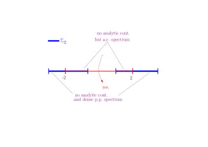
Figure 5. The analytic continuation of the resolvent and resonances for $H_{\omega}^{\infty}$

Let us also note here that if $0\in\,$supp$g$ (where $g$ is the density of the random variables defining the random potential), then, by (1.13), one has $[-2,2]\subset\Sigma$. In this case, there is no possibility to continue the resolvent of $H_{\omega}^{\infty}$ to the lower half plane passing through $[-2,2]$.
Comparing Theorem 1.13 to Theorem 1.5, we see that, as the operator $H^{\infty}$, when continued through $(-2,2)\cap\overset{\circ}{\Sigma}$, the operator $H^{\infty}_{\omega}$ does not have any resonances but for very different reasons.
When one does the continuation through $(-2,2)\setminus\Sigma$, one sees that the number of resonances is finite; “near” the real axis, the continuation of the function $\displaystyle E\mapsto 1-e^{i\theta(E)}\int_{\mathbb{R}}\frac{dN_{\omega}(\lambda)}{\lambda-E}$ has non trivial imaginary part and near $\infty$ it does not vanish.
Theorem 1.13 also shows that the equation studied in [26, 27], i.e., the equation $\Xi_{\omega}(E)=0$, does not describe the resonances of $H_{\omega}^{\infty}$ as is claimed in these papers: these resonances do not exist as there is no analytic continuation of the resolvent of $H_{\omega}^{\infty}$ through $(-2,2)\cap\Sigma$! As is shown in Theorem 1.12, the solutions to the equation $\Xi_{\omega}(E)=0$ give an approximation to the resonances of $H^{\mathbb{N}}_{\omega,L}$ (see Theorem 1.12).

1.4. Outline of and reading guide to the paper

In the present section, we shall explain the main ideas leading to the proofs of the results presented above.
In section 2, we prove Theorem 1.1; this proof is classical. As a consequence of the proof, one sees that, in the case of the half-lattice $\mathbb{N}$ (resp. lattice $\mathbb{Z}$), the resonances are the eigenvalues of a rank one (resp. two) perturbation of $(-\Delta+V)_{|\llbracket 0,L\rrbracket}$ with Dirichlet b.c. The perturbation depends in an explicit way on the resonance. This yields a closed equation for the resonances in terms of the eigenvalues and normalized eigenfunctions of the Dirichlet restriction $(-\Delta+V)_{|\llbracket 0,L\rrbracket}$. To obtain a description of the resonances we then are in need of a “precise” description of the eigenvalues and normalized eigenfunctions. Actually the only information needed on the normalized eigenfunctions is their weight at the point $L$ (and the point $0$ in the full lattice case), $0$ and $L$ being the endpoints of $\llbracket 0,L\rrbracket$.
In section 3, we solve the two equations obtained previously under the condition that the weight of the normalized eigenfunctions at $L$ (and $0$) be much smaller than the spacing between the Dirichlet eigenvalues. This condition entails that the resonance equation we want to solve essentially factorizes and become very easy to solve (see Theorems 3.1, 3.2 and 3.3), i.e., it suffices to solve it near any given Dirichlet eigenvalue.

For periodic potentials, the condition that the eigenvalue spacing is much larger than the weight of the normalized eigenfunctions at $L$ (and $0$) is not satisfied: both quantities are of the same order of magnitude (see Theorem 4.2) for the Dirichlet eigenvalues in the bulk of the spectrum, i.e., the vast majority of them. This is a consequence of the extended nature of the eigenfunctions in this case. Therefore, we find another way to solve the resonance equation. This way goes through a more precise description of the Dirichlet eigenvalues and normalized eigenfunctions which is the purpose of Theorems 4.2. We use this description to reduce the resonance equation to an effective equation (see Theorem 5.1) up to errors of order $O(L^{-\infty})$. It is important to obtain errors of at most that size. Indeed, the effective equation may have solutions to any order (the order is finite and only depends on $V$ but it is unknown); thus, to obtain solutions to the true equation from solutions to the effective equation with a good precision, one needs the two equations to differ by at most $O(L^{-\infty})$. We then solve the effective equation and, in section 5.2, prove the results of section 1.2.

On the other hand, for random potentials, it is well known that the eigenfunctions of the Dirichlet restriction $(-\Delta+V)_{|\llbracket 0,L\rrbracket}$ are exponentially localized and, for most of them localized, far from the edge of $\llbracket 0,L\rrbracket$. Thus, their weight at $L$ (and $0$ in the full lattice case) is typically exponentially small in $L$; the eigenvalue spacing however is typically of order $L^{-1}$. We can then use the results of section 3 to solve the resonance equation. The real part of a given resonance is directly related to a Dirichlet eigenvalue and its imaginary part to the weight of the corresponding eigenfunction at $L$ (and $0$ in the full lattice case). The main difficulty is to find the asymptotic behavior of this weight. Indeed, while it is known that, in the random case, eigenfunctions decay exponentially away from a localization center and while it is known that, for the full random Hamiltonian (i.e. the Hamiltonian on the line or half-line with a random potential), at infinity, this decay rate is given by the Lyapunov exponent, to the best of our knowledge, before the present work, it was not known at which length scale this Lyapunov behavior sets in (with a good probability). Answering this question is the purpose of Theorems 6.2 and 6.3 proved in section 6.3: we show that, for the $1$-dimensional Anderson model, for $\delta>0$ arbitrary, on a box of size $L$ sufficiently large, all the eigenfunctions exhibit an exponential decay (we obtain both an upper and a lower bound on the eigenfunctions) at a rate equal to the Lyapunov exponent at the corresponding energy (up to an error of size $\delta$) as soon as one is at a distance $\delta L$ from the corresponding localization center.
These bounds give estimates on the weight of most eigenfunctions at the point $L$ (and $0$ in the full lattice case): it is directly related to the distance of the corresponding localization center to the points $L$ (and $0$). One can then transform the known results on the statistics of the (rescaled) eigenvalues and (rescaled) localization centers into statistics of the (rescaled) resonances. This is done in section 6.2 and proves most of the results in section 1.3.
Finally, section 6.4 is devoted to the study of the full line Hamiltonian obtained from the free Hamiltonian on one half-line and a random Hamiltonian on the other half-line; it contains in particular the proof of Theorem 1.13.

2. The analytic continuation of the resolvent

Resonances for Jacobi matrices were considered in various works (see, e.g., [6, 16] and references tehrein). For the sake of completeness, we provide an independent proof of Theorem 1.1. It follows standard ideas that were first applied in the continuum setting, i.e., for partial differential operators instead of finite difference operators (see, e.g., [38] and references therein).
The proof relies on the fact that the resolvent of free Laplace operator can be continued holomorphically from $\mathbb{C}^{+}$ to $\displaystyle\mathbb{C}\setminus\left((-\infty,-2]\cup[2,+\infty)\right)$ as an operator valued function from $l^{2}_{\text{comp}}$ to $l^{2}_{\text{loc}}$. This is an immediate consequence of the fact that, by discrete Fourier transformation, $-\Delta$ is the Fourier multiplier by the function $\theta\mapsto 2\cos\theta$.
Indeed, for $-\Delta$ on $\ell^{2}(\mathbb{Z})$ and Im$\,E>0$, one has, for $(n,m)\in\mathbb{Z}$ (assume $n-m\geq 0$)

(2.1) $$\begin{split}\langle\delta_{n},(-\Delta-E)^{-1}\delta_{m}\rangle&=\frac{1}{2\pi}\int_{0}^{2\pi}\frac{e^{-i(n-m)\theta}}{2\cos\theta-E}d\theta=\frac{1}{2i\pi}\int_{|z|=1}\frac{z^{n-m}}{z^{2}-Ez+1}dz\\ &=\frac{1}{2\sqrt{(E/2)^{2}-1}}\left(E/2-\sqrt{(E/2)^{2}-1}\right)^{n-m}=\frac{e^{i(n-m)\theta(E)}}{\sin\theta(E)}\end{split}$$

where $E=2\cos\,\theta(E)$ and the determination $\theta=\theta(E)$ is chosen so that Im$\,\theta>0$ and Re$\,\theta\in(-\pi,0)$ for Im$\,E>0$. The determination satisfies $\displaystyle\theta\left(\overline{E}\right)=\overline{\theta(E)}$.
The map $E\mapsto\theta(E)$ can continued analytically from $\mathbb{C}^{+}$ to the cut plane $\displaystyle\mathbb{C}\setminus\left((-\infty,-2]\cup[2,+\infty)\right)$ as shown in Figure 6.

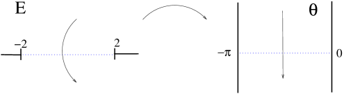
Figure 6. The mapping $E\mapsto\theta(E)$

The continuation is one-to-one and onto from $\displaystyle\mathbb{C}\setminus\left((-\infty,-2]\cup[2,+\infty)\right)$ to $(-\pi,0)+i\mathbb{R}$. It defines a determination of $E\mapsto\arccos(E/2)=\theta(E)$.
Clearly, using (2.1), this continuation yields an analytic continuation of $R_{0}^{\mathbb{Z}}:=(-\Delta-E)^{-1}$ from $\{$Im$\,E>0\}$ to $\displaystyle\mathbb{C}\setminus\left((-\infty,-2]\cup[2,+\infty)\right)$ as an operator from $l^{2}_{\text{comp}}$ to $l^{2}_{\text{loc}}$. Let us now turn to the half-line operator, i.e., $-\Delta$ on $\mathbb{N}$ with Dirichlet condition at $0$. Pick $E$ such that Im$\,E>0$ and set $E=2\cos\theta$ where the determination $\theta=\theta(E)$ is chosen as above. If for $v\in\mathbb{C}^{\mathbb{N}}$ bounded and $n\geq-1$, one sets $v_{-1}=0$ and

(2.2) $$[R_{0}^{\mathbb{N}}(E)(v)]_{n}=\frac{1}{2i\sin\theta(E)}\sum_{j=-1}^{n}v_{j}\cdot\sin((n-j)\theta(E))-e^{i\theta(E)}\frac{\sin((n+1)\theta(E))}{2i\sin\,\theta(E)}\sum_{j\geq 0}e^{ij\theta(E)}v_{j}.$$

Then, for Im$\,E>0$, a direct computations shows that

1. for $v\in\ell^{2}(\mathbb{N})$, the vector $R_{0}^{\mathbb{N}}(E)(v)$ is in the domain of the Dirichlet Laplacian on $\ell^{2}(\mathbb{N})$ , i.e., $[R_{0}^{\mathbb{N}}(E)(v)]_{-1}=0$;

2. for $n\geq 0$, one checks that

   (2.3) $$[R_{0}^{\mathbb{N}}(E)(v)]_{n+1}+[R_{0}^{\mathbb{N}}(E)(v)]_{n-1}-E[R_{0}^{\mathbb{N}}(E)(v)]_{n}=v_{n}.$$

3. $R_{0}^{\mathbb{N}}(E)$ defines a bounded map from $\ell^{2}(\mathbb{N})$ to itself;

Thus, $R_{0}^{\mathbb{N}}(E)$ is the resolvent of the Dirichlet Laplacian on $\mathbb{N}$ at energy $E$ for Im$\,E>0$. Using the continuation of $E\mapsto\theta(E)$, formula (2.2) yields an analytic continuation of the resolvent $R_{0}^{\mathbb{N}}(E)$ as an operator from $l^{2}_{\text{comp}}$ to $l^{2}_{\text{loc}}$.

Remark 2.1.

Note that the resolvent $R_{0}^{\mathbb{N}}(E)$ at an energy $E$ s.t. Im$\,E<0$ is given by formula (2.2) where $\theta(E)$ is replaced by $-\theta(E)$. For (2.2), one has to assume that $(v_{j})_{j\in\mathbb{N}}$ decays fast enough at $\infty$.

To deal with the perturbation $V$, we proceed in the same way on $\mathbb{Z}$ and on $\mathbb{N}$. Set $V^{L}=V\mathbf{1}_{\llbracket 0,L\rrbracket}$ (seen as a function on $\mathbb{N}$ or $\mathbb{Z}$ depending on the case). Letting $R_{0}(E)$ be either $R_{0}^{\mathbb{Z}}(E)$ or $R_{0}^{\mathbb{N}}(E)$, we compute

$$-\Delta+V^{L}-E=(-\Delta-E)(1+R_{0}(E)V^{L})=(1+V^{L}R_{0}(E))(-\Delta_{L}-E).$$

Thus, it suffices to check that the operator $R_{0}(E)V^{L}$ (resp. $V^{L}R_{0}(E)$) can be analytically continued as an operator from $l^{2}_{\text{loc}}$ to $l^{2}_{\text{loc}}$ (resp. $l^{2}_{\text{comp}}$ to $l^{2}_{\text{comp}}$). This follows directly from (2.2) and the fact $V^{L}$ has finite rank.
To complete the proof of Theorem 1.1, we just note that, as

• $E\mapsto R_{0}(E)V^{L}$ (resp. $E\mapsto V^{L}R_{0}(E)$) is a finite rank operator valued function analytic on the connected set $\displaystyle\mathbb{C}\setminus\left((-\infty,-2]\cup[2,+\infty)\right)$,

• $-1$ is not an eigenvalue of $R_{0}(E)V^{L}$ (resp. $V^{L}R_{0}(E)$) for Im$\,E>0$,

by the Fredholm principle, the set of energies $E$ for which $-1$ is an eigenvalue of $R_{0}(E)V^{L}$ (resp. $V^{L}R_{0}(E)$) is discrete. Hence, the set of resonances is discrete.
This completes the proof of the first part of Theorem 1.1. To prove the second part, we will first write a characteristic equation for resonances. The bound on the number of resonances will then be obtained through a bound on the number of solutions to this equation.

2.1. A characteristic equation for resonances

In the literature, we did not find a characteristic equation for the resonances in a form suitable for our needs. The characteristic equation we derive will take different forms depending on whether we deal with the half-line or the full line operator. But in both cases, the coefficients of the characteristic equation will be constructed from the spectral data (i.e. the eigenvalues and eigenfunctions) of the operator $H_{L}$ (see Remark 1.4).

2.2. In the half-line case

We first consider $H^{\mathbb{N}}_{L}$ on $\ell^{2}(\mathbb{N})$ and prove

Theorem 2.1.

Consider the operator $H_{L}$ defined as $H^{\mathbb{N}}_{L}$ restricted to $\llbracket 0,L\rrbracket$ with Dirichlet boundary conditions at $L$ and define

• $(\lambda_{j})_{0\leq j\leq L}=(\lambda_{j}(L))_{0\leq j\leq L}$ are the Dirichlet eigenvalues of $H^{\mathbb{N}}_{L}$ ordered so that $\lambda_{j}<\lambda_{j+1}$;

• $a^{\mathbb{N}}_{j}=a^{\mathbb{N}}_{j}(L)=|\varphi_{j}(L)|^{2}$ where $\varphi_{j}=(\varphi_{j}(n))_{0\leq n\leq L}$ is a normalized eigenvector associated to $\lambda_{j}$.

Then, an energy $E$ is a resonance of $H^{\mathbb{N}}_{L}$ if and only if

(2.4) $$S_{L}(E):=\sum_{j=0}^{L}\frac{a^{\mathbb{N}}_{j}}{\lambda_{j}-E}=-e^{-i\theta(E)},\quad E=2\cos\theta(E),$$

the determination of $\theta(E)$ being chosen so that Im$\,\theta(E)>0$ and Re$\,\theta(E)\in(-\pi,0)$ when Im$\,E>0$.

Let us note that

(2.5) $$\forall 0\leq j\leq L,\ a^{\mathbb{N}}_{j}(L)>0\quad\text{and}\quad\sum_{j=0}^{L}a^{\mathbb{N}}_{j}(L)=\sum_{j=0}^{L}|\varphi_{j}(L)|^{2}=1.$$

Proof of Theorem 2.1.

By the proof of the first statement of Theorem 1.1 (see the beginning of section 2), we know that an energy $E$ is a resonance if and only if $-1$ if an eigenvalue of $R_{0}(E)V^{L}$ where $R_{0}(E)$ is defined by (2.2). Pick $E$ an resonance and let $u=(u_{n})_{n\geq 0}$ be a resonant state that is an eigenvector of $R_{0}(E)V^{L}$ associated to the eigenvalue $-1$. As $V^{L}_{n}=0$ for $n\geq L+1$, equation (2.2) yields that, for $n\geq L+1$, $u_{n}=\beta e^{in\theta(E)}$ for some fixed $\beta\in\mathbb{C}^{*}$. As $u=-R_{0}(E)V^{L}u$, for $n\geq L+1$, it satisfies $u_{n+1}+u_{n-1}=E\,u_{n}$. Thus, $u_{L+1}=e^{i\theta(E)}u_{L}$ and by (2.3), $u$ is a solution to the eigenvalues problem

$$\begin{cases}u_{n+1}+u_{n-1}+V_{n}u_{n}=E\,u_{n},\ \forall n\in\llbracket 0,L\rrbracket\\ u_{-1}=0,\quad u_{L+1}=e^{i\theta(E)}u_{L}\end{cases}$$

This can be equivalently be rewritten as

(2.6) $$\begin{pmatrix}V_{0}&1&0&\cdots&0\\ 1&V_{1}&1&0&&\\ \vdots&\ddots&\ddots&\ddots&\\ &0&1&V_{L-1}&1\\ 0&\cdots&0&1&V_{L}+e^{i\theta(E)}\\ \end{pmatrix}\begin{pmatrix}u_{0}\\ \\ \vdots\\ \\ u_{L}\end{pmatrix}=E\begin{pmatrix}u_{0}\\ \\ \vdots\\ \\ u_{L}\end{pmatrix}$$

The matrix in (2.6) is the Dirichlet restriction of $H^{\mathbb{N}}_{L}$ to $\llbracket 0,L\rrbracket$ perturbed by the rank one operator $e^{i\theta(E)}\delta_{L}\otimes\delta_{L}$. Thus, by rank one perturbation theory (see, e.g., [36]), an energy $E$ is a resonance if and only if if satisfies (2.4).
This completes the proof of Theorem 2.1. ∎

Let us now complete the proof of Theorem 1.1 for the operator on the half-line. Let us first note that, for Im$\,E>0$, the imaginary part of the left hand side of (2.4) is positive by (2.7). On the other hand, the imaginary part of the right hand side of (2.4) is equal to $-e^{\text{Im}\,\theta(E)}\sin($Re$\,\theta(E))$ and, thus, is negative (recall that Re$\,\theta(E)\in(-\pi,0)$ (see fig. 1). Thus, as already underlined, equation (2.4) has no solution in the upper half-plane or on the interval $(-2,2)$.
Clearly, equation (2.4) is equivalent to the following polynomial equation of degree $2L+2$ in the variable $z=e^{-i\theta(E)}$

(2.7) $$\prod_{k=0}^{L}\left(z^{2}-2\lambda_{k}z+1\right)-\sum_{j=0}^{L}a^{\mathbb{N}}_{j}\prod_{\begin{subarray}{c}0\leq k\leq L\\ k\not=j\end{subarray}}\left(z^{2}-2\lambda_{k}z+1\right)=0.$$

We are looking for the solutions to (2.7) in the upper half-plane. As the polynomial in the right hand side of (2.7) has real coefficients, its zeros are symmetric with respect to the real axis. Moreover, one notices that, by (2.5), $0$ is a solution to (2.7). Hence, the number of solutions to (2.7) in the upper half-plane is bounded by $L$. This completes the proof of Theorem 1.1.

2.3. On the whole line

Now, consider $H^{\mathbb{Z}}_{L}$ on $\ell^{2}(\mathbb{Z})$. We prove

Theorem 2.2.

Using the notations of Theorem 2.1, an energy $E$ is a resonance of $H^{\mathbb{Z}}_{L}$ if and only if

(2.8) $$\text{det}\left(\sum_{j=0}^{L}\frac{1}{\lambda_{j}-E}\begin{pmatrix}|\varphi_{j}(L)|^{2}&\overline{\varphi_{j}(0)}\varphi_{j}(L)\\ \varphi_{j}(0)\overline{\varphi_{j}(L)}&|\varphi_{j}(0)|^{2}\end{pmatrix}+e^{-i\theta(E)}\right)=0$$

where $det(\cdot)$ denotes the determinant of a square matrix, $E=2\cos\theta(E)$ and the determination of $\theta(E)$ is chosen as in Theorem 2.1.

So, an energy $E$ is a resonance of $H^{\mathbb{Z}}_{L}$ if and only if $-e^{-i\theta(E)}$ belongs to the spectrum of the $2\times 2$ matrix

(2.9) $$\Gamma_{L}(E):=\sum_{j=0}^{L}\frac{1}{\lambda_{j}-E}\begin{pmatrix}|\varphi_{j}(L)|^{2}&\overline{\varphi_{j}(0)}\varphi_{j}(L)\\ \varphi_{j}(0)\overline{\varphi_{j}(L)}&|\varphi_{j}(0)|^{2}\end{pmatrix}.$$

Proof of Theorem 2.2.

The proof is the same as that of Theorem 2.1 except that now $E$ is a resonance if there exists $u$ a non trivial solution to the eigenvalues problem

$$\begin{cases}u_{n+1}+u_{n-1}+V_{n}u_{n}=E\,u_{n},\ \forall n\in\llbracket 0,L\rrbracket\\ u_{-1}=e^{i\theta(E)}u_{0}\text{ and }u_{L+1}=e^{i\theta(E)}u_{L}\end{cases}$$

This can be equivalently be rewritten as

$$\begin{pmatrix}V_{0}+e^{i\theta(E)}&1&0&\cdots&0\\ 1&V_{1}&1&0&&\\ \vdots&\ddots&\ddots&\ddots&\\ &0&1&V_{L-1}&1\\ 0&\cdots&0&1&V_{L}+e^{i\theta(E)}\\ \end{pmatrix}\begin{pmatrix}u_{0}\\ \\ \vdots\\ \\ u_{L}\end{pmatrix}=E\begin{pmatrix}u_{0}\\ \\ \vdots\\ \\ u_{L}\end{pmatrix}$$

Thus, using rank one perturbations twice, we find that an energy $E$ is a resonance if and only if

$$\left(1+e^{i\theta(E)}\sum_{j=0}^{L}\frac{|\varphi_{j}(0)|^{2}}{\lambda_{j}-E}\right)\left(1+e^{i\theta(E)}\sum_{j=0}^{L}\frac{|\varphi_{j}(L)|^{2}}{\lambda_{j}-E}\right)\\ =e^{2i\theta(E)}\sum_{0\leq j,j^{\prime}\leq L}\frac{\varphi_{j}(L)\varphi_{j^{\prime}}(0)\overline{\varphi_{j^{\prime}}(L)\varphi_{j}(0)}}{(\lambda_{j}-E)(\lambda_{j^{\prime}}-E)},$$

that is, if and only is (2.8) holds. This completes the proof of Theorem 2.2. ∎

Let us now complete the proof of Theorem 1.1 for the operator on the full-line. Let us first show that (2.8) has no solution in the upper half-plane. Therefore, if $-e^{-i\theta(E)}$ belongs to the spectrum of the matrix defined by (2.8) and if $u\in\mathbb{C}^{2}$ is a normalized eigenvector associated to $-e^{-i\theta(E)}$, one has

$$\sum_{j=0}^{L}\frac{1}{\lambda_{j}-E}\left|\left\langle\begin{pmatrix}\varphi_{j}(L)\\ \varphi_{j}(0)\end{pmatrix},u\right\rangle\right|^{2}=-e^{-i\theta(E)}.$$

This is impossible in the upper half-plane and on $(-2,2)$ as the two sides of the equation have imaginary parts of opposite signs.
Note that

$$\sum_{j=0}^{L}\begin{pmatrix}\varphi_{j}(L)\\ \varphi_{j}(0)\end{pmatrix}\overline{\begin{pmatrix}\varphi_{j}(L)&\varphi_{j}(0)\end{pmatrix}}=\begin{pmatrix}1&0\\ 0&1\end{pmatrix}.$$

Note also that $-e^{-i\theta(E)}$ is an eigenvalue of (2.8) if and only if it satisfies

(2.10) $$1+e^{i\theta(E)}\sum_{j=0}^{L}\frac{|\varphi_{j}(L)|^{2}+|\varphi_{j}(0)|^{2}}{\lambda_{j}-E}=-\frac{1}{2}e^{2i\theta(E)}\sum_{0\leq j,j^{\prime}\leq L}\frac{\left|\begin{matrix}\varphi_{j}(0)&\varphi_{j^{\prime}}(0)\\ \varphi_{j}(L)&\varphi_{j^{\prime}}(L)\end{matrix}\right|^{2}}{(\lambda_{j}-E)(\lambda_{j^{\prime}}-E)}.$$

As the eigenvalues of $H_{L}$ are simple, one computes

(2.11) $$\sum_{0\leq j,j^{\prime}\leq L}\frac{\left|\begin{matrix}\varphi_{j}(0)&\varphi_{j^{\prime}}(0)\\ \varphi_{j}(L)&\varphi_{j^{\prime}}(L)\end{matrix}\right|^{2}}{(\lambda_{j}-E)(\lambda_{j^{\prime}}-E)}=2\sum_{0\leq j\leq L}\frac{1}{\lambda_{j}-E}\sum_{j^{\prime}\not=j}\frac{1}{\lambda_{j^{\prime}}-\lambda_{j}}\left|\begin{matrix}\varphi_{j}(0)&\varphi_{j^{\prime}}(0)\\ \varphi_{j}(L)&\varphi_{j^{\prime}}(L)\end{matrix}\right|^{2}.$$

Thus, equation (2.10) is equivalent to the following polynomial equation of degree $2(L+1)$ in the variable $z=e^{-i\theta(E)}$

(2.12) $$z\prod_{k=0}^{L}\left(z^{2}-\lambda_{k}z+1\right)-\sum_{j=0}^{L}(2a^{\mathbb{Z}}_{j}z+b^{\mathbb{Z}}_{j})\prod_{\begin{subarray}{c}0\leq k\leq L\\ k\not=j\end{subarray}}\left(z^{2}-\lambda_{k}z+1\right)=0.$$

where we have defined

(2.13) $$\begin{split}a^{\mathbb{Z}}_{j}&:=\frac{1}{2}\left(|\varphi_{j}(L)|^{2}+|\varphi_{j}(0)|^{2}\right)=\frac{1}{2}\left\|\begin{pmatrix}\varphi_{j}(L)\\ \varphi_{j}(0)\end{pmatrix}\right\|^{2}=\frac{1}{2}\left\|\begin{pmatrix}|\varphi_{j}(L)|^{2}&\overline{\varphi_{j}(0)}\varphi_{j}(L)\\ \varphi_{j}(0)\overline{\varphi_{j}(L)}&|\varphi_{j}(0)|^{2}\end{pmatrix}\right\|.\end{split}$$

and

$$b^{\mathbb{Z}}_{j}:=\sum_{j^{\prime}\not=j}\frac{1}{\lambda_{j^{\prime}}-\lambda_{j}}\left|\begin{matrix}\varphi_{j}(0)&\varphi_{j^{\prime}}(0)\\ \varphi_{j}(L)&\varphi_{j^{\prime}}(L)\end{matrix}\right|^{2}.$$

The sequence $(a^{\mathbb{Z}}_{j})_{j}$ also satisfies (2.5). Taking $|E|$ to $+\infty$ in (2.11), one notes that

(2.14) $$\sum_{j=0}^{L}b^{\mathbb{Z}}_{j}=0\quad\text{and}\quad\sum_{j=0}^{L}\lambda_{j}b^{\mathbb{Z}}_{j}=-\frac{1}{2}\sum_{0\leq j,j^{\prime}\leq L}\left|\begin{matrix}\varphi_{j}(0)&\varphi_{j^{\prime}}(0)\\ \varphi_{j}(L)&\varphi_{j^{\prime}}(L)\end{matrix}\right|^{2}=-1.$$

We are looking for the solutions to (2.12) in the upper half-plane. As the polynomial in the right hand side of (2.12) has real coefficients, its zeros are symmetric with respect to the real axis. Moreover, one notices that, by (2.14), $0$ is a root of order two of the polynomial in (2.12). Hence, as the polynomial has degree $2L+3$, the number of solutions to (2.12) in the upper half-plane is bounded by $L$. This completes the proof of Theorem 1.1.

3. General estimates on resonances

By Theorems 2.1 and 2.2, we want to solve equations (2.4) and (2.8) in the lower half-plane. We first derive some general estimates for zones in the lower half-plane free of solutions to equations (2.4) and (2.8) (i.e. resonant free zones for the operators $H^{\mathbb{N}}_{L}$ and $H^{\mathbb{Z}}_{L}$) and later a result on the existence of solutions to equations (2.4) and (2.8) (i.e. resonances for the operators $H^{\mathbb{N}}_{L}$ and $H^{\mathbb{Z}}_{L}$).

3.1. General estimates for resonant free regions

We keep the notations of Theorems 2.1 and 2.2. To simplify the notations in the theorems of this section, we will write $a_{j}$ for either $a^{\mathbb{N}}_{j}$ when solving (2.4) or $a^{\mathbb{Z}}_{j}$ when solving (2.8). We will specify the superscript only when there is risk of confusion.
We first prove

Theorem 3.1.

Fix $\delta>0$. Then, there exists $C>0$ (independent of $V$ and $L$) such that, for any $L$ and $j\in\{0,\cdots,L\}$ such that $-4+\delta\leq\lambda_{j-1}+\lambda_{j}<\lambda_{j+1}+\lambda_{j}\leq 4-\delta$, equations (2.4) and (2.8) have no solution in the set

(3.1) $$U_{j}:=\left\{E\in\mathbb{C};\ \begin{aligned} \text{Re}\,E&\in\left[\frac{\lambda_{j}+\lambda_{j-1}}{2},\frac{\lambda_{j}+\lambda_{j+1}}{2}\right]\\ \quad 0\geq C\cdot\theta^{\prime}_{\delta}\,&\text{Im}\,E>-a_{j}\,d^{2}_{j}\,|\sin\,\text{Re}\;\theta(E)|\end{aligned}\right\}$$

where the map $E\mapsto\theta(E)$ is defined in section 2 and we have set

(3.2) $$d_{j}:=\min\left(\lambda_{j+1}-\lambda_{j},\lambda_{j}-\lambda_{j-1},1\right)\quad\text{and}\quad\theta^{\prime}_{\delta}:=\max_{|E|\leq 2-\frac{\delta}{2}}|\theta^{\prime}(E)|.$$

Figure 7. The resonance free zones $U_{j}$ and $\tilde{U}_{j}$.

In Theorem 3.1 there are no conditions on the numbers $(a_{j})_{j}$ or $(d_{j})_{j}$ except their being positive. In our application to resonances, this holds. Theorem 3.1 becomes optimal when $a_{j}\ll d^{2}_{j}$. In our application to resonances, for periodic operators, one has $a_{j}\asymp L^{-1}$ and $d_{j}\asymp L^{-1}$ (see Theorem 5.2) and for random operators, one has $a_{j}\asymp e^{-cL}$ and $d_{j}\gtrsim L^{-4}$ (see Theorem 6.2 and (6.10)). Thus, in the random case, Theorem 3.1 will provide an optimal strip free of resonances whereas in the periodic case we will use a much more precise computation (see Theorem 5.1) to obtain sharp results.
When $a_{j}\ll d_{j}^{2}$, one proves the existence of another resonant free region near a energy $\lambda_{j}$, namely,

Theorem 3.2.

Fix $\delta>0$. Pick $j\in\{0,\cdots,L\}$ such that $-4+\delta<\lambda_{j-1}+\lambda_{j}<\lambda_{j+1}+\lambda_{j}<4-\delta$. There exists $C>0$ (depending only on $\delta$) such that, for any $L$, if $a_{j}\leq d^{2}_{j}/C^{2}$, equations (2.4) and (2.8) have no solution in the set

(3.3) $$\begin{split}\tilde{U}_{j}&:=\left\{E\in\mathbb{C};\ \begin{split}\text{Re}\,E&\in\left[\frac{\lambda_{j}+\lambda_{j-1}}{2},\lambda_{j}-Ca_{j}\right]\cup\left[\lambda_{j}+Ca_{j},\frac{\lambda_{j}+\lambda_{j+1}}{2}\right]\\ \quad&-Ca_{j}\leq\text{Im}\,E\leq-a_{j}\,d^{2}_{j}/C\end{split}\right\}\\ &\hskip 85.35826pt\bigcup\left\{E\in\mathbb{C};\ \begin{split}\text{Re}\,E&\in\left[\frac{\lambda_{j}+\lambda_{j-1}}{2},\frac{\lambda_{j}+\lambda_{j+1}}{2}\right]\\ \quad&-d^{2}_{j}/C\leq\text{Im}\,E\leq-Ca_{j}\end{split}\right\}\end{split}$$

Theorem 3.2 becomes optimal when $a_{j}$ is small and $d_{j}$ is of order one. This will be sufficient to deal with the isolated eigenvalues for both the periodic and the random potential. It will also be sufficient to give a sharp description of the resonant free region for random potentials. For the periodic potential, we will rely a much more precise computations (see Theorem 5.1).
Note that Theorem 3.2 guarantees that, if $d_{j}$ is not too small, outside $R_{j}$, resonances are quite far below the real axis.

Proof of Theorem 3.1.

The basic idea of the proof is that, for $E$ close to $\lambda_{j}$, $S_{L}(E)$ and the matrix $\Gamma_{L}(E)$ are either large or have a very small imaginary part while, as $-4<\lambda_{j-1}+\lambda_{j}<\lambda_{j+1}+\lambda_{j}<4$, $e^{-i\theta(E)}$ has a large imaginary part. Thus, (2.4) and (2.8) have no solution in this region.
We start with equation (2.4). Pick $E\in U_{j}$ for some $C$ large to be chosen later on. Assume first that $|E-\lambda_{j}|\leq a_{j}d_{j}(2+C_{0}d_{j})^{-1}$ for $C_{0}:=2e^{1/C}$. Recall that $0<a_{j},d_{j}\leq 1$. Note that, for $C$ sufficiently large, for $E\in U_{j}$, one has

(3.4) $$\begin{split}\left|\text{Im}\,e^{-i\theta(E)}\right|&=e^{\text{Im}\,\theta(E)}|\sin\text{Re}\,\theta(E)|=e^{\text{Im}[\theta(E)-\theta(\text{Re}\,E)]}|\sin\text{Re}\,\theta(E)|\\ &\geq e^{\theta^{\prime}_{\delta}\text{Im}E}|\sin\text{Re}\,\theta(E)|\geq e^{-1/C}|\sin\text{Re}\,\theta(E)|\end{split}$$

and

(3.5) $$\left|e^{-i\theta(E)}\right|\leq 1\leq e^{1/C}.$$

One estimates

(3.6) $$|S_{L}(E)|\geq\frac{a_{j}}{|\lambda_{j}-E|}-\sum_{k\not=j}\frac{a_{k}}{|\lambda_{k}-E|}\geq\frac{2}{d_{j}}+C_{0}-\sum_{k\not=j}\frac{2a_{k}}{\displaystyle\min_{k\not=j}|\lambda_{k}-\lambda_{j}|}\geq C_{0}=2e^{1/C}.$$

Thus, comparing (3.6) and (3.5), we see that equation (2.4) has no solution in the set $U_{j}\cap\{|E-\lambda_{j}|\leq a_{j}d_{j}(2+Cd_{j})^{-1}\}$.
Assume now that $|E-\lambda_{j}|>a_{j}d_{j}(2+C_{0}d_{j})^{-1}$. Then, for $E\in U_{j}$, one has

(3.7) $$|\text{Im}\,E|\leq\frac{1}{\theta^{\prime}_{\delta}C}a_{j}d^{2}_{j}|\sin(\text{Re}\,\theta(E))|.$$

Thus, for $E\in U_{j}\cap\{|E-\lambda_{j}|>a_{j}d_{j}(2+C_{0}d_{j})^{-1}\}$, one computes

(3.8) $$\begin{split}|\text{Im}\,S_{L}(E)|&\leq|\text{Im}\,E|\left(\frac{a_{j}}{|\lambda_{j}-\text{Re}\,E|^{2}+|\text{Im}\,E|^{2}}+\frac{4}{d^{2}_{j}+|\text{Im}\,E|^{2}}\right)\\ &\leq\frac{1}{\theta^{\prime}_{\delta}C}a_{j}d^{2}_{j}|\sin(\text{Re}\,\theta(E))|\left(\frac{(2+C_{0}d_{j})^{2}a_{j}}{a^{2}_{j}d^{2}_{j}}+\frac{4}{d_{j}^{2}}\right)\\ &\leq\frac{4}{\theta^{\prime}_{\delta}C}(1+e^{1/C})^{2}|\sin(\text{Re}\,\theta(E))|\leq\frac{1}{2}e^{-1/C}|\sin(\text{Re}\,\theta(E))|\end{split}$$

provided $C$ satisfies $\displaystyle 8e^{1/C}(1+e^{1/C})^{2}<\theta^{\prime}_{\delta}C$.
Hence, the comparison of (3.4) with (3.8) shows that (2.4) has no solution in $U_{j}\cap\{|E-\lambda_{j}|>a_{j}d_{j}(2+C_{0}d_{j})^{-1}\}$ if we choose $C$ large enough (independent of $(a_{j})_{j}$ and $(\lambda_{j})_{j}$). Thus, we have proved that for some $C>0$ large enough (independent of $(a_{j})_{j}$ and $(\lambda_{j})_{j}$),  (2.4) has no solution in $U_{j}$. Let us now turn to the case of equation (2.8). The basic ideas are the same as for equation (2.4). Consider the matrix $\Gamma_{L}(E)$ defined by (2.9). The summands in (2.9) are hermitian, of rank $1$ and their norm is given by (2.13).
Assume that $E\in U_{j}$ is a solution to (2.8). Define the vectors

$$v_{j}:=a_{j}^{-1/2}\begin{pmatrix}\varphi_{j}(L)\\ \varphi_{j}(0)\end{pmatrix}\quad\text{for}\quad j\in\{0,\cdots,L\}.$$

Here $a_{j}=a_{j}^{\mathbb{Z}}$.
Note that by definition of $a_{j}$, one has $\|v_{j}\|^{2}=2$. Pick $u$ in $C^{2}$, a normalized eigenvector of $\Gamma_{L}(E)$ associated to the eigenvalue $-e^{-i\theta(E)}$. Thus, $u$ satisfies

(3.9) $$\sum_{j=0}^{L}\frac{a_{j}\,\langle v_{j},u\rangle\,v_{j}}{\lambda_{j}-E}=-e^{-i\theta(E)}u$$

Note that, by assumption, one has

(3.10) $$\sup_{E\in U_{j}}\left\|\sum_{k\not=j}\frac{a_{k}\,\langle v_{k},u\rangle\,v_{k}}{\lambda_{k}-E}\right\|\lesssim\frac{1}{d_{j}}\quad\text{and}\quad\left|\text{Im}\left(\sum_{k\not=j}\frac{a_{k}\,|\langle v_{k},u\rangle|^{2}}{\lambda_{k}-E}\right)\right|\lesssim\frac{|\text{Im}\,E|}{d^{2}_{j}}$$

where the constants are independent of $C$, the one defining $U_{j}$.
Taking the (real) scalar product of equation (3.9) with $\overline{u}$, and then the imaginary part, we obtain

$$-\frac{a_{j}\,|\langle v_{j},u\rangle|^{2}\text{Im}\,E}{|\lambda_{j}-E|^{2}}+\text{Im}\left(e^{-i\theta(E)}\right)=O\left(\frac{|\text{Im}\,E|}{d^{2}_{j}}\right)$$

Thus, for $E\in U_{j}$, as $a_{j}\leq 1$, for $C$ in (3.1) sufficiently large (depending only on $\delta$),

$$\frac{a_{j}\,|\langle v_{j},u\rangle|^{2}|\text{Im}\,E|}{|\lambda_{j}-E|^{2}}\geq\frac{1}{2}|\sin(\text{Re}\,\theta(E))|.$$

Hence, for a solution to (2.8) in $U_{j}$ and $u$ as above, one has

$$|\lambda_{j}-E|\leq|\langle v_{j},u\rangle|\sqrt{\frac{2a_{j}|\text{Im}\,E|}{|\sin(\text{Re}\,\theta(E))|}}\leq 2\sqrt{\frac{a_{j}|\text{Im}\,E|}{|\sin(\text{Re}\,\theta(E))|}}.$$

Hence, by the definition of $U_{j}$, for $C$ large, we get

(3.11) $$\left|\frac{a_{j}}{\lambda_{j}-E}\right|\geq\frac{C\theta^{\prime}_{\delta}}{d_{j}}\gg\frac{1}{d_{j}}.$$

By (3.10), the operator $\Gamma_{L}(E)$ can be written as

(3.12) $$\Gamma_{L}(E)=\frac{a_{j}}{\lambda_{j}-E}v_{j}\otimes v_{j}+R_{j}(E)+iI_{j}(E)$$

where $R_{j}(E)$ and $I_{j}(E)$ are self-adjoint ($I_{j}$ is non negative) and satisfy

(3.13) $$\|R_{j}(E)\|\lesssim\frac{1}{d_{j}}\quad\text{ and }\quad\|I_{j}(E)\|\lesssim\frac{|\text{Im}\,E|}{d^{2}_{j}}.$$

An explicit computation shows that the eigenvalues of the two-by-two matrix $\displaystyle\frac{a_{j}}{\lambda_{j}-E}v_{j}\otimes v_{j}+R_{j}(E)$ satisfy

$$\text{either}\quad\lambda=\frac{a_{j}}{\lambda_{j}-E}\left(1+O\left(\frac{d_{j}}{C\theta^{\prime}_{\delta}}\right)\right)\quad\text{or}\quad|\text{Im}\,\lambda|\lesssim\frac{|\operatorname{Im}E|}{a_{j}}$$

where the implicit constants are independent of the one defining $U_{j}$.
Thus, by (3.12), using (3.11) and the second estimate in (3.13), we see that the eigenvalues of the matrix $\displaystyle\Gamma_{L}(E)$ satisfy

$$\text{either}\quad\lambda=\frac{a_{j}}{\lambda_{j}-E}\left(1+O\left(\frac{d_{j}}{C\theta^{\prime}_{\delta}}\right)\right)\quad\text{or}\quad|\text{Im}\,\lambda|\leq\frac{2}{C\theta^{\prime}_{\delta}}.$$

Clearly, for $C$ large, no such value can be equal to $-e^{-i\theta(E)}$ being to large by (3.11) in the first case or having too small imaginary part in the second. The proof of Theorem 3.1 is complete. ∎

Proof of Theorem 3.2.

Again, we start with the solutions to (2.4). For $z\in\tilde{U}_{j}$, we compute

(3.14) $$\begin{split}\text{Im}\,S_{L}(E)&=\sum_{k=0}^{L}\frac{a_{k}\,\text{Im}\,E}{(\lambda_{k}-\text{Re}\,E)^{2}+\text{Im}^{2}E}\\ &=\frac{a_{j}\,\text{Im}\,E}{(\lambda_{j}-\text{Re}\,E)^{2}+\text{Im}^{2}E}+\sum_{\begin{subarray}{c}0\leq k\leq L\\ k\not=j\end{subarray}}\frac{-a_{k}\,\text{Im}\,E}{(\lambda_{k}-\text{Re}\,E)^{2}+\text{Im}^{2}E}.\end{split}$$

When $-d^{2}_{j}/C\leq\text{Im}\,E\leq-Ca_{j}$, the second equality above and (2.5) yield, for $C$ sufficiently large,

(3.15) $$0\leq\text{Im}\,S_{L}(E)\lesssim\frac{a_{j}}{|\text{Im}\,E|}+\frac{|\text{Im}\,E|}{d^{2}_{j}+\text{Im}^{2}E}\leq\frac{2}{C}.$$

On the other hand, for some $K>0$, one has

$$\left|\text{Im}\,e^{-i\theta(E)}\right|\geq|\text{Im}\,e^{-i\theta(\text{Re}\,E)}|-Kd^{2}_{j}/C.$$

Now, as, under the assumptions of Theorem 3.2, one has

(3.16) $$\min_{E\in\left[\frac{\lambda_{j}+\lambda_{j-1}}{2},\frac{\lambda_{j}+\lambda_{j+1}}{2}\right]}\left|\text{Im}\,e^{-i\theta(E)}\right|\geq\frac{1}{4}\min\left(\sqrt{16-(\lambda_{j}+\lambda_{j-1})^{2}},\sqrt{16-(\lambda_{j}+\lambda_{j+1})^{2}}\right),$$

we obtain that (2.4) has no solution in $\tilde{U}_{j}\cap\{-d_{j}/C\leq\text{Im}\,E\leq-Ca_{j}\}$.
Pick now $E\in\tilde{U}_{j}$ such that $-Ca_{j}\leq\text{Im}\,E\leq-a_{j}d_{j}^{2}/C$. Then, (3.5) and (2.5) yield, for $C$ sufficiently large,

$$\text{Im}\,S_{L}(E)\lesssim\frac{a_{j}\text{Im}\,E}{C^{2}a^{2}_{j}+\text{Im}^{2}E}+\frac{Ca_{j}}{d^{2}_{j}}\leq\frac{1}{C}+\frac{1}{2C}.$$

The imaginary part of $e^{-i\theta(E)}$ is estimated as above. Thus, for $C$ sufficiently large,  (2.4) has no solution in $\tilde{U}_{j}\cap\{-Ca_{j}\leq\text{Im}\,E\leq-a_{j}d_{j}^{2}/C\}$.The case of equation (2.8) is studied in exactly the same way except that, as in the proof of Theorem 3.1, one has to replace the study of $S_{L}(E)$ by that of $\langle\Gamma_{L}(E)u,u\rangle$ for $u$ a normalized eigenvector of $\Gamma_{L}(E)$ associated to $-e^{-i\theta(E)}$ and, thus, the coefficient $a_{k}$ in (3.14) gets multiplied by a factor $|\langle v_{k},u\rangle|^{2}$ that is bounded by $2$.
This completes the proof of Theorem 3.2. ∎

3.2. The resonances near an “isolated” eigenvalue

We will now solve equation (2.4) near a given $\lambda_{j}$ under the additional assumptions that $a_{j}\ll d^{2}_{j}$. By Theorems 3.1 and 3.2, we will do so in the rectangle $R_{j}$ (see Fig. 7). Actually, we prove that, in $R_{j}$, there is exactly one resonance and give an asymptotic for this resonance in terms of $a_{j}$, $d_{j}$ and $\lambda_{j}$. This result is going to be applied to the case of random $V$ and to that of isolated eigenvalues (for any $V$).
Using the notations of section 3, for $j\in\{0,\cdots,L\}$, we define

(3.17) $$S_{L,j}(E):=\sum_{k\not=j}\frac{a^{\mathbb{N}}_{k}}{\lambda_{k}-E}\quad\text{and}\quad\Gamma_{L,j}(E):=\sum_{k\not=j}\frac{1}{\lambda_{k}-E}\begin{pmatrix}|\varphi_{k}(L)|^{2}&\overline{\varphi_{k}(0)}\varphi_{k}(L)\\ \varphi_{k}(0)\overline{\varphi_{k}(L)}&|\varphi_{k}(0)|^{2}\end{pmatrix}.$$

We prove

Theorem 3.3.

Pick $j\in\{0,\cdots,L\}$ such that $-4<\lambda_{j-1}+\lambda_{j}<\lambda_{j+1}+\lambda_{j}<4$. There exists $C>1$ (depending only on $(\lambda_{j-1}+\lambda_{j})+4$ and $4-(\lambda_{j+1}+\lambda_{j})$) such that, for any $L$, if $a_{j}\leq d^{2}_{j}/C$, equation (2.4) and (2.8) has exactly one solution in the set

(3.18) $$R_{j}:=\left\{E\in\mathbb{C};\ \begin{aligned} \text{Re}\,E&\in\lambda_{j}+Ca_{j}\left[-1,1\right]\\ \quad-Ca_{j}\leq&\text{Im}\,E\leq-a_{j}\,d^{2}_{j}/C\end{aligned}\right\}.$$

Moreover, the solution to (2.4), say $z^{\mathbb{N}}_{j}$, satisfies

(3.19) $$z^{\mathbb{N}}_{j}=\lambda_{j}+\frac{a^{\mathbb{N}}_{j}}{S_{L,j}(\lambda_{j})+e^{-i\theta(\lambda_{j})}}+O\left(\left(a^{\mathbb{N}}_{j}d^{-1}_{j}\right)^{2}\right).$$

and the solution to (2.8), say $z^{\mathbb{Z}}_{j}$, satisfies

(3.20) $$z^{\mathbb{Z}}_{j}=\lambda_{j}+\left\langle\begin{pmatrix}\overline{\varphi_{j}(L)}\\ \varphi_{j}(0)\end{pmatrix},\left(\Gamma_{L,j}(\lambda_{j})+e^{-i\theta(\lambda_{j})}\right)^{-1}\begin{pmatrix}\overline{\varphi_{j}(L)}\\ \varphi_{j}(0)\end{pmatrix}\right\rangle+O\left(\left(a^{\mathbb{Z}}_{j}d^{-1}_{j}\right)^{2}\right).$$

Note that, if $a^{\mathbb{N}}_{j}d^{-2}_{j}$ is small, formula (3.19) gives the asymptotic of the width of the solution $z^{\mathbb{N}}_{j}$, namely,

(3.21) $$\text{Im}\,z^{\mathbb{N}}_{j}=\frac{a^{\mathbb{N}}_{j}\cdot\sin\theta(\lambda_{j})}{[S_{L,j}(\lambda_{j})+\cos\theta(\lambda_{j})]^{2}+\sin^{2}\theta(\lambda_{j})}(1+o(1)).$$

Recall that $\sin\theta(\lambda_{j})<0$ (see Theorem 2.1). For $H_{L}^{\mathbb{Z}}$, using the bounds (3.28) and (3.29), we see that the asymptotic of the imaginary part of the solution $z^{\mathbb{Z}}_{j}$ satisfies

(3.22) $$-\frac{1}{C}a^{\mathbb{Z}}_{j}\leq\text{Im}\,z^{\mathbb{Z}}_{j}\leq-Ca^{\mathbb{Z}}_{j}d_{j}^{2}.$$

This and (3.21) will be useful when $a_{j}\ll d^{2}_{j}$ as will be the case for random potentials. The case when $a_{j}$ and $d_{j}$ are of the same order of magnitude requires more information. This is the case that we meet in the next section when dealing with periodic potentials.
The proof of Theorem 3.3 also yields the behavior of the functions $E\mapsto S_{L}(E)+e^{-i\theta(E)}$ and $\displaystyle E\mapsto\text{det}\left(\Gamma_{L}(E)+e^{-i\theta(E)}\right)$ near their zeros in $R_{j}$ and, in particular shows the following

Proposition 3.1.

Fix $\delta>0$. Under the assumptions of Theorem 3.3, there exists $c>0$ such that, for $-4+\delta<\lambda_{j-1}+\lambda_{j}<\lambda_{j+1}+\lambda_{j}<4-\delta$, one has

$$\inf_{0<r<ca^{\mathbb{N}}_{j}d^{-1}_{j}}\min_{|E-z^{\mathbb{N}}_{j}|=r}\frac{\left|S_{L}(E)+e^{-i\theta(E)}\right|}{r} \geq c\quad\text{and}$$

$$\inf_{0<r<ca^{\mathbb{Z}}_{j}d^{-1}_{j}}\min_{|E-z^{\mathbb{Z}}_{j}|=r}\frac{\left|\text{det}\left(\Gamma_{L}(E)+e^{-i\theta(E)}\right)\right|}{r} \geq c.$$

Proposition 3.1 is a consequence of the analogues of (3.24) and (3.30) on the rectangles

$$\tilde{R}_{j}=\tilde{z}_{j}+ca^{\bullet}_{j}d^{-1}_{j}[-1,1]\times[-1,1]$$

for $\bullet\in\{\mathbb{N},\mathbb{Z}\}$ and $c$ sufficiently small.

Proof of Theorem 3.3.

Let us start with equation (2.4). To prove the statement on equation (2.4), in $R_{j}$, we compare the function $E\mapsto S_{L}(E)+e^{-i\theta(E)}$ to the function

$$E\mapsto\tilde{S}_{L,j}(E)=\frac{a^{\mathbb{N}}_{j}}{\lambda_{j}-E}+S_{L,j}(\lambda_{j})+e^{-i\theta(\lambda_{j})}.$$

Clearly, in $\mathbb{C}$, the equation $\tilde{S}_{L,j}(E)=0$ admits a unique solution given by

$$\tilde{z}_{j}=\lambda_{j}+\frac{a^{\mathbb{N}}_{j}}{S_{L,j}(\lambda_{j})+e^{-i\theta(\lambda_{j})}}.$$

For $E\in\partial R_{j}$, the boundary of $R_{j}$, one has

(3.23) $$\begin{split}\left|\tilde{S}_{L,j}(E)\right|\geq\frac{1}{2C}\quad&\text{and}\quad\left|\frac{a^{\mathbb{N}}_{j}}{\lambda_{j}-E}\right|\geq\frac{1}{2C},\\ \left|e^{-i\theta(E)}-e^{-i\theta(\lambda_{j})}\right|\leq Ca^{\mathbb{N}}_{j}&\quad\text{and}\quad\left|S_{L,j}(E)-S_{L,j}(\lambda_{j})\right|\leq Ca^{\mathbb{N}}_{j}d^{-2}_{j}.\end{split}$$

Hence, as $d_{j}\leq 1$, one gets

$$\max_{E\in\partial R_{j}}\frac{\left|\tilde{S}_{L,j}(E)-S_{L}(E)-e^{-i\theta(E)}\right|}{|\tilde{S}_{L,j}(E)|}\leq 4Ca^{\mathbb{N}}_{j}d_{j}^{-2}$$

Thus, by Rouché’s theorem, equation (2.4) has a unique solution in $R_{j}$.
To obtain the asymptotics of the solution, it suffices to use Rouché’s theorem again with the functions $\tilde{S}_{L,j}$ and $S_{L}(E)+e^{-i\theta(E)}$ on the smaller rectangle $\tilde{R}_{j}=\tilde{z}_{j}+K(a^{\mathbb{N}}_{j}d^{-1}_{j})^{2}[-1,1]\times[-1,1]$. One then estimates

(3.24) $$\max_{E\in\partial\tilde{R}_{j}}\frac{\left|\tilde{S}_{L,j}(E)-S_{L}(E)-e^{-i\theta(E)}\right|}{|\tilde{S}_{L,j}(E)|}\leq 4CK^{-1}.$$

Thus, for $K$ sufficiently large, this completes the proof of the statements on the solutions to equation (2.4) contained in Theorem 3.3.Let us turn to equation (2.8). On $R_{j}$, we now compare $\Gamma_{L}(E)+e^{-i\theta(E)}$ to the matrix valued function

$$E\mapsto\tilde{\Gamma}_{L,j}(E):=\frac{1}{\lambda_{j}-E}\begin{pmatrix}|\varphi_{j}(L)|^{2}&\overline{\varphi_{j}(0)}\varphi_{j}(L)\\ \varphi_{j}(0)\overline{\varphi_{j}(L)}&|\varphi_{j}(0)|^{2}\end{pmatrix}+\Gamma_{L,j}(\lambda_{j})+e^{-i\theta(\lambda_{j})}.$$

The matrix $\displaystyle\begin{pmatrix}|\varphi_{j}(L)|^{2}&\overline{\varphi_{j}(0)}\varphi_{j}(L)\\ \varphi_{j}(0)\overline{\varphi_{j}(L)}&|\varphi_{j}(0)|^{2}\end{pmatrix}$ is rank $1$ and can be diagonalized as

$$\begin{pmatrix}|\varphi_{j}(L)|^{2}&\overline{\varphi_{j}(0)}\varphi_{j}(L)\\ \varphi_{j}(0)\overline{\varphi_{j}(L)}&|\varphi_{j}(0)|^{2}\end{pmatrix}=P_{j}\begin{pmatrix}a^{\mathbb{Z}}_{j}&0\\ 0&0\end{pmatrix}P^{*}_{j}$$

where $a^{\mathbb{Z}}_{j}$ is given by (2.13) and

$$P_{j}=\frac{1}{\sqrt{a^{\mathbb{Z}}_{j}}}\begin{pmatrix}\varphi_{j}(L)&-\overline{\varphi_{j}(0)}\\ \varphi_{j}(0)&\overline{\varphi_{j}(L)}\end{pmatrix}.$$

Thus, $\tilde{\Gamma}_{L,j}(E)$ is unitarily equivalent to

(3.25) $$M:=\frac{1}{\lambda_{j}-E}\begin{pmatrix}a^{\mathbb{Z}}_{j}&0\\ 0&0\end{pmatrix}+P_{j}^{*}\Gamma_{L,j}(\lambda_{j})P_{j}+e^{-i\theta(\lambda_{j})}.$$

As $P_{j}^{*}\Gamma_{L,j}(\lambda_{j})P_{j}$ is real and the imaginary part of $e^{-i\theta(\lambda_{j})}$ does not vanish, the matrix $M_{0}:=P_{j}^{*}\Gamma_{L,j}(\lambda_{j})P_{j}+e^{-i\theta(\lambda_{j})}$ is invertible. By rank $1$ perturbation theory (see , e.g., [37]), we know that $M$ is invertible if and only if $a^{\mathbb{Z}}_{j}\left[M_{0}^{-1}\right]_{11}+\lambda_{j}\not=E$ (where $[M]_{11}$ is the upper right coefficient of the $2\times 2$ matrix $M$). In this case, one has

(3.26) $$M^{-1}=M_{0}^{-1}-\frac{a^{\mathbb{Z}}_{j}}{a^{\mathbb{Z}}_{j}\left[M_{0}^{-1}\right]_{11}+\lambda_{j}-E}M_{0}^{-1}\begin{pmatrix}1&0\\ 0&0\end{pmatrix}M_{0}^{-1}.$$

Hence, $0$ is an eigenvalue of $M$ if and only if

(3.27) $$\begin{split}E&=\lambda_{j}+a^{\mathbb{Z}}_{j}\left[\left(P_{j}^{*}\Gamma_{L,j}(\lambda_{j})P_{j}+e^{-i\theta(\lambda_{j})}\right)^{-1}\right]_{11}\\ &=\lambda_{j}+\left\langle\begin{pmatrix}\overline{\varphi_{j}(L)}\\ \varphi_{j}(0)\end{pmatrix},\left(\Gamma_{L,j}(\lambda_{j})+e^{-i\theta(\lambda_{j})}\right)^{-1}\begin{pmatrix}\overline{\varphi_{j}(L)}\\ \varphi_{j}(0)\end{pmatrix}\right\rangle.\end{split}$$

Note that, as $\Gamma_{L,j}(\lambda_{j})$ is real symmetric and $\|\Gamma_{L,j}(\lambda_{j})\|\leq Cd_{j}^{-1}$, one has

(3.28) $$\left|\left\langle\begin{pmatrix}\overline{\varphi_{j}(L)}\\ \varphi_{j}(0)\end{pmatrix},\left(\Gamma_{L,j}(\lambda_{j})+e^{-i\theta(\lambda_{j})}\right)^{-1}\begin{pmatrix}\overline{\varphi_{j}(L)}\\ \varphi_{j}(0)\end{pmatrix}\right\rangle\right|\leq\frac{a^{\mathbb{Z}}_{j}}{\left|\sin\theta(\lambda_{j})\right|}.$$

and

(3.29) $$\text{Im}\left(\left\langle\begin{pmatrix}\overline{\varphi_{j}(L)}\\ \varphi_{j}(0)\end{pmatrix},\left(\Gamma_{L,j}(\lambda_{j})+e^{-i\theta(\lambda_{j})}\right)^{-1}\begin{pmatrix}\overline{\varphi_{j}(L)}\\ \varphi_{j}(0)\end{pmatrix}\right\rangle\right)\leq\frac{a^{\mathbb{Z}}_{j}d_{j}^{2}\sin\theta(\lambda_{j})}{1+d_{j}^{2}}.$$

Using (3.25), (3.26), (3.28) and (3.29),we see that, for $E\in\partial R_{j}$, the boundary of $R_{j}$, $\tilde{\Gamma}_{L,j}(E)$ is invertible and that one has

$$\left\|\left[\tilde{\Gamma}_{L,j}(E)\right]^{-1}\right\|\leq 2C\quad\text{and}\quad\left\|\Gamma_{L,j}(E)-\Gamma_{L,j}(\lambda_{j})\right\|\leq Ca^{\mathbb{Z}}_{j}d^{-2}_{j}.$$

Hence, as $d_{j}\leq 1$, taking (3.23) into account, one gets

$$\max_{E\in\partial R_{j}}\left\|1-\left[\tilde{\Gamma}_{L,j}(E)\right]^{-1}\left(\Gamma_{L}(E)+e^{-i\theta(E)}\right)\right\|\leq 4C^{2}a^{\mathbb{Z}}_{j}d_{j}^{-2}$$

In the same way, one proves

(3.30) $$\max_{E\in\partial\tilde{R}_{j}}\left\|1-\left[\tilde{\Gamma}_{L,j}(E)\right]^{-1}\left(\Gamma_{L}(E)+e^{-i\theta(E)}\right)\right\|\lesssim K^{-1}$$

where we recall that $\tilde{R}_{j}=\tilde{z}_{j}+K(a^{\mathbb{N}}_{j}d^{-1}_{j})^{2}[-1,1]\times[-1,1]$.
Thus, we can apply Rouché’s Theorem to compare the following two functions on $\partial R_{j}$ and $\partial\tilde{R}_{j}$ (for $K$ sufficiently large),

$$\text{det}\left(\tilde{\Gamma}_{L,j}(E)\right)\quad\text{and}\quad\text{det}\left(\Gamma_{L}(E)+e^{-i\theta(E)}\right)$$

as

$$\frac{\left|\text{det}\left(\tilde{\Gamma}_{L,j}(E)\right)-\text{det}\left(\Gamma_{L}(E)+e^{-i\theta(E)}\right)\right|}{\left|\text{det}\left(\tilde{\Gamma}_{L,j}(E)\right)\right|}\\ =\left|1-\text{det}\left(1-\left[1-\left[\tilde{\Gamma}_{L,j}(E)\right]^{-1}\left(\Gamma_{L}(E)+e^{-i\theta(E)}\right)\right]\right)\right|.$$

We then conclude as in the case of equation (2.4). This completes the proof of Theorem 3.3. ∎

Combining Theorems 3.3, 3.1 and 3.2, we get a pretty clear picture of the resonances near the Dirichlet eigenvalues in $(-2,2)$ as long as the associated $a_{j}$ and $d_{j}$ behave correctly. As said, this and the knowledge of the spectral statistics for random operators will enable us to prove the results described in section 1.3. For the periodic case, Theorems 3.1, 3.2 and 3.3 will prove not too be sufficient. As we shall see, in this case, $a_{j}$ and $d_{j}$ are of the same order of magnitude. Thus, neighboring Dirichlet eigenvalues have a sizable effect on the location of resonances. Therefore, in the next section, we compute the Dirichlet spectral data for the truncated periodic potential.

4. The Dirichlet spectral data for periodic potentials

As we did not find any suitable reference for this material, we first derive a suitable description of the spectral data (i.e. the $(a_{j})_{j}$ and $(\lambda_{j})_{j}$) for the Dirichlet restriction of a periodic operator to the interval $\llbracket 0,L\rrbracket$ when $L$ becomes large.
Consider a potential $V:\mathbb{N}\to\mathbb{R}$ such that, for some $p\geq 1$, one has $V_{k}=V_{k+p}$ for all $k\geq 0$. We assume $p$ to be minimal, i.e., to be the period of $V$. In our first result, we describe the spectrum of $H^{\mathbb{Z}}=-\Delta+V$ on $\ell^{2}(\mathbb{Z})$ and $H^{\mathbb{N}}=-\Delta+V$ on $\ell^{2}(\mathbb{N})$ (with Dirichlet boundary conditions at $0$). In the second result we turn to $H_{L}$, the Dirichlet restriction $H^{\mathbb{N}}$ to $\llbracket 0,L\rrbracket$ and described its spectral data, i.e., its eigenvalues and eigenfunctions.
We recall

Theorem 4.1.

The spectrum of $H^{\mathbb{Z}}$, say $\Sigma_{\mathbb{Z}}$, is a union of at most $p$ disjoint intervals that all consist in purely absolutely continuous spectrum.
The spectrum of $H^{\mathbb{N}}$ is the union of $\Sigma_{\mathbb{Z}}$ and at most finitely many simple eigenvalues outside $\Sigma_{\mathbb{Z}}$, say, $(v_{j})_{0\leq j\leq n}$. $\Sigma_{\mathbb{Z}}$ consists of purely absolutely continuous spectrum of $H^{\mathbb{N}}$ and the eigenfunctions associated to $(v_{j})_{0\leq j\leq n}$, say $(\psi_{j})_{0\leq j\leq n}$, are exponentially decaying at infinity.

Except for the exponential decay of the eigenfunctions, the proof of the statement for the periodic operator on $\mathbb{Z}$ and $\mathbb{N}$ is classical and can e.g. be found in a more general setting in [39, chapters 2, 3 and 7] (see also [42, 35]). The exponential decay is an immediate consequence of Floquet theory for the periodic Hamiltonian on $\mathbb{Z}$ and the fact that the eigenvalues lie in gaps of $\Sigma_{\mathbb{Z}}$.
For $H^{\mathbb{Z}}$ one can define its Bloch quasi-momentum (see the beginning of section 4.1 for details) that we denote by $\theta_{p}$; it is continuous and strictly increasing on $\Sigma_{\mathbb{Z}}$ and real analytic on $\overset{\circ}{\Sigma}_{\mathbb{Z}}$. Decompose $\Sigma_{\mathbb{Z}}$ into its connected components, i.e., $\displaystyle\Sigma_{\mathbb{Z}}=\bigcup_{r=1}^{q}B_{r}$ where $q\leq p$. Let $c_{q}$ be the number of closed gaps contained in $q$. Then, $\theta_{p}$ is continuous and strictly increasing on $B_{r}$ and real analytic on $\overset{\circ}{B}_{r}$, the interior of the $r$-th band. Moreover, on this set, its derivative can be expressed in terms of the density of states defined in (1.2) as

(4.1) $$n(\lambda)=\frac{1}{\pi}\theta^{\prime}_{p}(\lambda).$$

We first describe the eigenvalues of $H_{L}$.

Theorem 4.2.

One has

1. For any $k\in\{0,\cdots,p-1\}$, there exists $h_{k}:\;\Sigma_{\mathbb{Z}}\to\mathbb{R}$, a continuous function that is real analytic in a neighborhood of $\overset{\circ}{\Sigma}_{\mathbb{Z}}$ such that, for $L$ sufficiently large s.t. $L\equiv k\mod p$,

   1. for $1\leq r\leq q$, the function $h_{k}$ maps $B_{r}$ into $(-(c_{r}+1)\pi,(c_{r}+1)\pi)$;

   2. define the function

      (4.2) $$\theta_{p,L}:=\theta_{p}-\frac{h_{k}}{L-k};$$

      it is continuous and strictly monotonous on each $B_{r}$ ($1\leq r\leq q$);

   3. for $1\leq r\leq q$, the eigenvalues of $H_{L}$ in $B_{r}$, the $r$-th band of $\Sigma_{\mathbb{Z}}$, say $(\lambda^{r}_{j})_{j}$, are the solutions (in $\Sigma_{\mathbb{Z}}$) to the quantization conditions

      (4.3) $$\theta_{p,L}(\lambda^{r}_{j})=\frac{j\pi}{L-k},\quad j\in\mathbb{Z}.$$

2. There exists $c>0$ such that, if $\lambda$ is an eigenvalue of $H_{L}$ outside $\Sigma_{\mathbb{Z}}$, then, for $L=Np+k$ sufficiently large, there exists $\lambda_{\infty}\in\Sigma_{0}^{+}\cup\Sigma^{-}_{k}\setminus\Sigma_{\mathbb{Z}}$ s.t., one has $|\lambda-\lambda_{\infty}|\leq e^{-cL}$.

Recall that $\Sigma_{0}^{+}$ and $\Sigma^{-}_{k}$ are respectively the spectra of $H_{0}^{+}$ and $H^{-}_{k}$ defined in section 1.2.2.
In Theorem 4.2, when solving equation (4.3), one has to do it for each band $B_{r}$, and, for each band and each $j$ such that $\displaystyle\frac{j\pi}{L-k}\in\theta_{p,L}(B_{r})$, equation (4.3) admits a unique solution. But, it may happen that one has two solutions to (4.3) for a given $j$ belonging to neighboring bands. In the sequel to simplify the notations, we will not distinguish between the different bands, i.e., we will write eigenvalues $(\lambda_{j})_{j}$ not referring to the band they belong to.
Let us now describe the associated eigenfunctions.

Theorem 4.3.

Recall that $(\lambda_{j})_{j}$ are the eigenvalues of $H_{L}$ in $\Sigma_{\mathbb{Z}}$ (enumerated as in Theorem 4.2).

1. There exist $p+2$ positive functions, say, $f^{+}_{0}$, $(f^{-}_{k})_{0\leq k\leq p-1}$ and $\tilde{f}$, that are real analytic in a neighborhood of $\overset{\circ}{\Sigma}_{\mathbb{Z}}$ such that, there exists $\sigma_{r}\in\{+1,-1\}$ such that, for $L=Np+k$ sufficiently large, for $\lambda_{j}$ in $\overset{\circ}{B_{r}}$, the interior of $r$-th band of $\Sigma_{\mathbb{Z}}$, one has

   (4.4) $$\begin{split}&|\varphi_{l}(L)|^{2}=\frac{f^{-}_{k}(\lambda_{j})}{L-k}\left(1+\frac{\tilde{f}(\lambda_{j})}{L-k}\right)^{-1},\quad|\varphi_{l}(0)|^{2}=\frac{f^{+}_{0}(\lambda_{j})}{f^{-}_{k}(\lambda_{j})}|\varphi_{l}(L)|^{2},\\ &\varphi_{l}(L)\overline{\varphi_{l}(0)}=\sigma_{r}\,e^{i\pi l}|\varphi_{l}(L)||\varphi_{l}(0)|=\sigma_{r}\,e^{i(L-k)\theta_{p}(\lambda_{j})-h_{k}(\lambda_{j})}|\varphi_{l}(L)||\varphi_{l}(0)|.\end{split}$$

2. Let $\lambda$ be an eigenvalue of $H_{L}$ outside $\Sigma_{\mathbb{Z}}$ (see point (3) in Theorem 4.2). If $\varphi$ is a normalized eigenfunction associated to $\lambda$ and $H_{L}$, one has one of the following alternatives for $L$ large

   1. if $\lambda_{\infty}\in\Sigma_{0}^{+}\setminus\Sigma^{-}_{k}$, one has

      (4.5) $$|\varphi(L)|\asymp e^{-cL}\quad\text{and}\quad|\varphi(0)|\asymp 1;$$

   2. if $\lambda_{\infty}\in\Sigma^{-}_{k}\setminus\Sigma^{+}_{0}$, one has

      (4.6) $$|\varphi(L)|\asymp 1\quad\text{and}\quad|\varphi(0)|\asymp e^{-cL};$$

   3. if $\lambda_{\infty}\in\Sigma^{-}_{k}\cap\Sigma^{+}_{0}$, one has

      (4.7) $$|\varphi(L)|\asymp 1\quad\text{and}\quad|\varphi(0)|\asymp 1.$$

For later use, let us define $\theta_{p,L}$, $f_{0,L}$ and $f_{k,L}$ by

(4.8) $$f_{k,L}(\lambda)=f^{-}_{k}(\lambda)\left(1+\frac{\tilde{f}(\lambda)}{L-k}\right)^{-1}\quad\text{and}\quad f_{0,L}(\lambda)=f^{+}_{0}(\lambda)\left(1+\frac{\tilde{f}(\lambda)}{L-k}\right)^{-1}$$

where $\theta_{p}$, $h_{k}$, $f_{0}$, $f_{k}$ and $\tilde{f}$ are defined in Theorem 4.2.
As a consequence of Theorem 4.2, we obtain

Corollary 4.1.

For $\lambda\in\overset{\circ}{\Sigma}_{\mathbb{Z}}$, for $L\equiv k\mod(p)$ sufficiently large, one has

(4.9) $$\frac{dN_{k}^{-}}{d\lambda}(\lambda)=n_{k}^{-}(\lambda)=f^{-}_{k}(\lambda)n(\lambda)=\frac{1}{\pi}f^{-}_{k}(\lambda)\theta_{p}^{\prime}(\lambda)=\frac{1}{\pi}f_{k,L}(\lambda)\theta_{p,L}^{\prime}(\lambda),$$

(4.10) $$\frac{dN_{0}^{+}}{d\lambda}(\lambda)=n_{0}^{+}(\lambda)=f^{+}_{0}(\lambda)n(\lambda)=\frac{1}{\pi}f^{+}_{0}(\lambda)\theta_{p}^{\prime}(\lambda)=\frac{1}{\pi}f_{0,L}(\lambda)\theta_{p,L}^{\prime}(\lambda).$$

Here, $\theta_{P}$, $f^{+}_{0}$ and $f^{-}_{k}$ are defined the functions defined in Theorem 4.2.

Proof of Corollary 4.1.

To prove the first equalities in (4.9) and (4.10), it suffices to prove that, for any $\chi\in{\mathcal{C}}_{0}^{\infty}(\overset{\circ}{\Sigma}_{\mathbb{Z}})$,

(4.11) $$\begin{aligned} \langle\delta_{0},\chi(H_{k}^{-})\delta_{0}\rangle&=\int_{\mathbb{R}}\chi(\lambda)dN_{k}^{-}(\lambda)=\frac{1}{\pi}\int_{\mathbb{R}}\chi(\theta_{p}^{-1}(k))f^{-}_{k}(\theta_{p}^{-1}(k))dk\\ &=\frac{1}{\pi}\int_{\mathbb{R}}\chi(\lambda)f^{-}_{k}(\lambda)\theta_{p}^{\prime}(\lambda)d\lambda,\end{aligned}$$

(4.12) $$\begin{aligned} \langle\delta_{0},\chi(H_{0}^{+})\delta_{0}\rangle&=\int_{\mathbb{R}}\chi(\lambda)dN_{0}^{+}(\lambda)=\frac{1}{\pi}\int_{\mathbb{R}}\chi(\theta_{p}^{-1}(k))f^{+}_{0}(\theta_{p}^{-1}(k))dk\\ &=\frac{1}{\pi}\int_{\mathbb{R}}\chi(\lambda)f^{+}_{0}(\lambda)\theta_{p}^{\prime}(\lambda)d\lambda,\end{aligned}$$

the full statement then following by standard density argument. The operator $H_{L}$ converges to $H_{0}^{+}$ in norm resolvent sense. Thus, we know that $\displaystyle\langle\delta_{0},\chi(H_{0}^{+})\delta_{0}\rangle=\lim_{L\to+\infty}\langle\delta_{0},\chi(H_{L})\delta_{0}\rangle$. Now, by Theorem 4.2, as $\chi$ is supported in $\overset{\circ}{\Sigma}_{\mathbb{Z}}$, using the Poisson formula, one computes

$$\begin{split}\langle\delta_{0},&\chi(H_{L})\delta_{0}\rangle=\sum_{j}\chi(\lambda_{j})||\varphi_{j}(0)|^{2}=\frac{1}{L-k}\sum_{l}\chi\left(\theta_{p,L}^{-1}\left(\frac{l\pi}{L-k}\right)\right)f_{0,L}\left(\theta_{p,L}^{-1}\left(\frac{l\pi}{L-k}\right)\right)\\ &=\frac{1}{L-k}\sum_{j\in\mathbb{Z}}\int_{\mathbb{R}}e^{-i2\pi j\lambda}\chi\left(\theta_{p,L}^{-1}\left(\frac{\pi\,\lambda}{L-k}\right)\right)f_{0,L}\left(\theta_{p,L}^{-1}\left(\frac{\pi\,\lambda}{L-k}\right)\right)d\lambda\\ &=\frac{1}{\pi}\sum_{j\in\mathbb{Z}}\int_{\mathbb{R}}e^{-i2(L-k)j\theta_{p,L}(\lambda)}\chi\left(\lambda\right)f_{0,L}\left(\lambda\right)\theta^{\prime}_{p,L}(\lambda)d\lambda.\end{split}$$

Thus, using the non stationary phase, i.e., integrating by parts, one gets, for any $N\geq 2$,

(4.13) $$\begin{split}\left|\langle\delta_{0},\chi(H_{L})\delta_{0}\rangle-\frac{1}{\pi}\int_{\mathbb{R}}\chi\left(\lambda\right)f_{0,L}\left(\lambda\right)\theta^{\prime}_{p,L}(\lambda)d\lambda\right|&\leq\sum_{j\geq 1}C_{N,K}\|\chi\|_{\mathcal{C}^{N}}(|j|(L-k))^{-N}\\ &\leq C_{N,K}\|\chi\|_{\mathcal{C}^{N}}((L-k))^{-N}.\end{split}$$

Here, we have used the analyticity of the functions $\theta_{p,L}$ and $f_{0,L}$.
To deal with $H_{k}^{-}$, we recall the operator $\tilde{H}_{L}$ (that is unitarily equivalent to $H_{L}$) defined in Remark 1.4. One has $\langle\delta_{L},H_{L}\delta_{L}\rangle=\langle\delta_{0},\chi(\tilde{H}_{L})\delta_{0}\rangle$, thus, as $H_{k}^{-}$ is the strong resolvent sense limit of $\tilde{H}_{L}$, one gets $\displaystyle\langle\delta_{0},\chi(H_{k}^{-})\delta_{0}\rangle=\lim_{L\to+\infty}\langle\delta_{L},\chi(H_{L})\delta_{L}\rangle$.
Then, (4.11) and (4.12) and, thus, the first equalities in (4.9) and (4.10), follow as $\theta^{\prime}_{p,L}$, $f_{0,L}$ and $f_{k,L}$ converge (locally uniformly on $\overset{\circ}{\Sigma}_{\mathbb{Z}}$) respectively to $\theta^{\prime}_{p}$, $f^{+}_{0}$ and $f^{-}_{k}$ (see (4.8) and Theorem 4.2).
Let us now prove the second equalities in (4.9) and (4.10). Therefore, we use an almost analytic extension (see [30]) of $\chi$, say, $\tilde{\chi}$, that is, a function $\tilde{\chi}:\ \mathbb{C}\to\mathbb{C}$ satisfying (

1. for $z\in\mathbb{R}$, $\tilde{\chi}(z)=\chi(z)$,

2. supp$(\tilde{\chi})\subset\{z\in\mathbb{C};\ |\text{Im}(z)|<1\}$,

3. $\tilde{\chi}\in{\mathcal{S}}(\{z\in\mathbb{C};\ |\text{Im}(z)|<1\})$,

4. The family of functions $\displaystyle x\mapsto\frac{\partial\tilde{\chi}}{\partial\overline{z}}(x+iy)\cdot|y|^{-n}$ (for $0<|y|<1$) is bounded in ${\mathcal{S}}(\mathbb{R})$ for any $n\in{\mathbb{N}}$.

Moreover, $\tilde{\chi}$ can be chosen so that one has the following estimates: for $n\geq 0$, $\alpha\geq 0$, $\beta\geq 0$, there exists $C_{n,\alpha,\beta}>0$ such that

(4.14) $$\sup_{0<|y|\leq 1}\sup_{x\in\mathbb{R}}\left|x^{\alpha}\frac{\partial^{\beta}}{\partial x^{\beta}}\left(|y|^{-n}\cdot\frac{\partial\tilde{\chi}}{\partial\overline{z}}(x+iy)\right)\right|\\ \leq C_{n,\alpha,\beta}\sup_{\begin{subarray}{c}\beta^{\prime}\leq n+\beta+2\alpha^{\prime}\leq\alpha\end{subarray}}\sup_{x\in\mathbb{R}}\left|x^{\alpha^{\prime}}\frac{\partial^{\beta^{\prime}}\chi}{\partial x^{\beta^{\prime}}}(x)\right|.$$

By the definition of $\chi$, the right hand side of (4.14) is bounded uniformly in $E$ complex.
Let $\chi\in{\mathcal{C}}_{0}^{\infty}(\mathbb{R})$ and $\tilde{\chi}$ be an almost analytic extension of $\chi(x)$. Then, by [15] and [20], we know that, for any $n$ and $\omega\in\Omega$, the following formula hold,

(4.15) $$\chi(H_{\bullet})=\frac{i}{2\pi}\int_{\mathbb{C}}\frac{\partial\tilde{\chi}}{\partial{\overline{z}}}(z)\cdot(z-H_{\bullet})^{-1}dz\wedge d{\overline{z}}$$

where $H_{\bullet}=H_{L},\ \tilde{H}_{L},\ H_{0}^{+}$ or $H_{k}^{-}$.
Using the geometric resolvent equation (see, e.g., [19, Theorem 5.20]) and the Combes-Thomas estimate (see , e.g., [19, Theorem 11.2]), we know that for some $C>0$, for Im$z\not=0$,

(4.16) $$\left|\left\langle\delta_{0},\left[(\tilde{H}_{L}-z)^{-1}-(H_{k}^{-}-z)^{-1}\right]\delta_{0}\right\rangle\right|\\ +\left|\left\langle\delta_{0},\left[(H_{L}-z)^{-1}-(H_{0}^{+}-z)^{-1}\right]\delta_{0}\right\rangle\right|\leq\frac{C}{|\text{Im}z|}e^{-L|\text{Im}z|/C}.$$

Plugging (4.16) into (4.15) and using (4.14), we get

$$\left|\sum_{j=0}^{L}\chi(\lambda_{j})|\varphi_{j}(0)|^{2}-\int_{\mathbb{R}}\chi(\lambda)dN^{+}_{0}(\lambda)\right|\leq\tilde{C}_{N}\int_{|y|\leq 1}|y|^{N-1}e^{-L|y|/C}dy\leq C_{N}L^{-N}$$

Thus, by (4.12) and (4.13), we obtain that, for $\chi\in{\mathcal{C}}_{0}^{\infty}(\overset{\circ}{\Sigma}_{\mathbb{Z}})$ and any $N\geq 0$, there exists $C_{N}>0$ such that

(4.17) $$\begin{split}&\left|\int_{\mathbb{R}}\chi\left(\lambda\right)\left[f_{0,L}\left(\lambda\right)\theta^{\prime}_{p,L}(\lambda)-f^{+}_{0}\left(\lambda\right)\theta^{\prime}_{p}(\lambda)\right]d\lambda\right|\\ &=\left|\int_{\mathbb{R}}\chi\left(\lambda\right)f_{0,L}\left(\lambda\right)\theta^{\prime}_{p,L}(\lambda)d\lambda-\int_{\mathbb{R}}\chi(\lambda)dN^{+}_{0}(\lambda)\right|\leq C_{N}L^{-N}.\end{split}$$

Now, by (4.3) and (4.8), the function $f_{0,L}\theta^{\prime}_{p,L}-f^{+}_{0}\theta^{\prime}_{p}$ admits an expansion in inverse powers of $L$ that is converging uniformly on compact subsets of $\overset{\circ}{\Sigma}_{\mathbb{Z}}$, namely,

$$f_{0,L}\theta^{\prime}_{p,L}-f^{+}_{0}\theta^{\prime}_{p}=\sum_{k\geq 1}L^{-k}\alpha_{k}.$$

Thus, (4.17) immediately yields that, for any $k\geq 1$, one has $\alpha_{k}\equiv 0$ on $\overset{\circ}{\Sigma}_{\mathbb{Z}}$. Hence, $f_{0,L}\theta^{\prime}_{p,L}\equiv f^{+}_{0}\theta^{\prime}_{p}$ on $\overset{\circ}{\Sigma}_{\mathbb{Z}}$. This completes the proof of Corollary 4.1. ∎

4.1. The proofs of Theorems 4.2 and 4.3

We will first describe some objects from the spectral theory of $H^{\mathbb{Z}}$, use them to describe the spectral theory of $H^{\mathbb{N}}$, prove Theorem 4.2 and finally prove Theorem 4.3.

4.1.1. The spectral theory of $H^{\mathbb{Z}}$

This material is classical (see, e.g., [42, 39]); we only recall it for the readers convenience. For $0\leq j\leq p-1$, define $\tilde{T}_{j}=\tilde{T}_{j}(E)$ to be a monodromy matrix for the periodic finite difference operator $H^{\mathbb{Z}}$, that is ,

(4.18) $$\tilde{T}_{j}(E)=T_{j+p-1,j}(E)=T_{j+p-1}(E)\cdots T_{j}(E)=:\begin{pmatrix}a^{j}_{p}(E)&b^{j}_{p}(E)\\ a^{j}_{p-1}(E)&b^{j}_{p-1}(E)\end{pmatrix}$$

where

(4.19) $$T_{j}(E)=\begin{pmatrix}E-V_{j}&-1\\ 1&0\end{pmatrix}.$$

The coefficients of $\tilde{T}_{j}(E)$ are monic polynomials in the energy $E$: $a^{j}_{p}(E)$ has degree $p$ and $b^{j}_{p}(E)$ has degree $p-1$. Clearly, det$\,\tilde{T}_{j}(E)=1$. As $j\mapsto V_{j}$ is $p$-periodic, so is $j\mapsto\tilde{T}_{j}(E)$. Moreover, for $j^{\prime}<j$, one has

(4.20) $$\tilde{T}_{j}(E)\,T_{j,j}(E)=T_{j+p-1,j^{\prime}+p-1}(E)\,\tilde{T}_{j^{\prime}}(E)=T_{j,j^{\prime}}(E)\,\tilde{T}_{j^{\prime}}(E).$$

Thus, the discriminant $\underline{\Delta}(E):=\,$tr$\,\tilde{T}_{j}(E)=a^{j}_{p}(E)+b^{j}_{p-1}(E)$ is a polynomial of degree $p$ that is independent of $j$; so are $\rho(E)$ and $\rho^{-1}(E)$, the eigenvalues of $\tilde{T}_{j}(E)$. One defines the Bloch quasi-momentum $E\mapsto\theta_{p}(E)$ by

(4.21) $$\underline{\Delta}(E)=\rho(E)+\rho^{-1}(E)=2\cos(p\,\theta_{p}(E)).$$

Let us recall some basic properties of the discriminant $\Delta$ and the coefficients of $\tilde{T}_{j}$, the proofs of which can be found in [42]:

1. if $\Delta^{\prime}(E)=0$ then $|\underline{\Delta}(E)|\geq 2$;

2. the zeros of $\Delta^{\prime}$ are simple;

3. $E$ is a zero of $\Delta^{\prime}$ s.t. $|\underline{\Delta}(E)|=2$ if and only if $\tilde{T}_{j}(E)\in\{+\,$Id,$-\,$Id$\}$ (for any $j$);

4. the polynomials $b_{p}^{j}$ and $a_{p-1}^{j}$ only vanish in the set $\{|\underline{\Delta}(E)|\geq 2\}$ ; they keep a fixed sign in each of the connected components of the set $\{|\underline{\Delta}(E)|<2\}$.

Note that $\underline{\Delta}(E)$ is real when $E$ is real. Thus, for $E$ real, $|\underline{\Delta}(E)|\leq 2$ implies that $\rho^{-1}(E)=\overline{\rho(E)}$ and $|\underline{\Delta}(E)|>2$ that $\rho(E)$ is real. When $|\underline{\Delta}(E)|\leq 2$, we will fix $\rho(E):=e^{ip\theta_{p}(E)}$ and when $|\underline{\Delta}(E)|>2$, we will fix $\rho(E)$ so that $|\rho(E)|<1$.
$E$ belongs to the spectrum of $H^{\mathbb{Z}}$ (i.e. $-\Delta+V$ on $\ell^{2}(\mathbb{Z})$) if and only if $|\underline{\Delta}(E)|\leq 2$ (see, e.g., [39]).
Properties (1)-(3) above imply that, for $E_{0}$ a zero of $\Delta^{\prime}$ such that $\underline{\Delta}(E_{0})=\pm 2$, $\theta_{p}$ is real analytic near $E_{0}$ and $\theta^{\prime}_{p}(E_{0})\not=0$.

Definition 4.1.

$E_{0}$ is said to be a closed gap if and only if $|\underline{\Delta}(E_{0})|=2$ and $\Delta^{\prime}(E_{0})=0$ or equivalently if and only if $\tilde{T}_{0}(E_{0})$ is diagonal.

Consider $\partial\Sigma_{\mathbb{Z}}$. It is the set of energies solutions to $|\underline{\Delta}(E)|=2$ where $\tilde{T}_{0}(E)$ is not diagonal; it is also the set of roots of $|\underline{\Delta}(E)|=2$ that are not closed gaps. From the upper half of the complex plane, one can continue $E\mapsto\theta_{p}(E)$ analytically to the universal cover of $\mathbb{C}\setminus\partial\Sigma_{\mathbb{Z}}$. Each of the points in $\partial\Sigma_{\mathbb{Z}}$ is a branch point of $\theta_{p}$ of square root type. Moreover, for $E\not\in\partial\Sigma_{\mathbb{Z}}$, there exists two linearly independent solutions to the eigenvalue equation $(-\Delta+V-E)u=0$, say $\varphi_{\pm}(E)$, satisfying, for $n\in\mathbb{Z}$

(4.22) $$\varphi_{\pm}(n+p,E)=e^{\pm ip\theta_{p}(E)}\varphi_{\pm}(n,E).$$

4.1.2. The spectral theory of $H^{\mathbb{N}}$

Let us now turn to the spectrum of the operator on the half-lattice.

The operator $H_{0}^{+}$

For the operator $H_{0}^{+}=H^{\mathbb{N}}$ (that is $-\Delta+V$ on $\ell^{2}(\mathbb{N})$ with Dirichlet boundary conditions at $0$), $E$ is in the spectrum if and only if

• either $|\underline{\Delta}(E)|\leq 2$

• or $|\underline{\Delta}(E)|>2$ and $\displaystyle[\tilde{T}_{0}(E)]^{n}\begin{pmatrix}1\\ 0\end{pmatrix}$ stays bounded as $n\to+\infty$.

The second condition is equivalent to asking that $\displaystyle[\tilde{T}_{j}(E)]^{n}T_{j-1}(E)\cdots T_{0}(E)\begin{pmatrix}1\\ 0\end{pmatrix}$ stay bounded as $n\to+\infty$.
When $|\underline{\Delta}(E)|\not=2$ and $a^{0}_{p-1}(E)\not=0$, one can diagonalize $\tilde{T}_{0}(E)$ in the following way

(4.23) $$\begin{pmatrix}a^{0}_{p-1}(E)&\rho(E)-a^{0}_{p}(E)\\ -a^{0}_{p-1}(E)&a^{0}_{p}(E)-\rho^{-1}(E)\end{pmatrix}\times\tilde{T}_{0}(E)\\ =\begin{pmatrix}\rho(E)&0\\ 0&\rho^{-1}(E)\end{pmatrix}\times\begin{pmatrix}a^{0}_{p-1}(E)&\rho(E)-a^{0}_{p}(E)\\ -a^{0}_{p-1}(E)&a^{0}_{p}(E)-\rho^{-1}(E)\end{pmatrix}.$$

Thus, using

(4.24) $$\left|\begin{matrix}\rho(E)-a_{p}^{0}(E)&-b_{p}^{0}(E)\\ -a_{p-1}^{0}(E)&\rho(E)-b_{p-1}^{0}(E)\end{matrix}\right|=\left|\begin{matrix}\rho(E)-a_{p}^{0}(E)&-b_{p}^{0}(E)\\ -a_{p-1}^{0}(E)&a_{p}^{0}(E)-\rho^{-1}(E)\end{matrix}\right|=0$$

for $n\in\mathbb{Z}$, one computes

(4.25) $$\left(\tilde{T}_{0}(E)\right)^{n}=\begin{pmatrix}\tilde{t}_{0,n}^{11}(E)&\tilde{t}_{0,n}^{12}(E)\\ \tilde{t}_{0,n}^{21}(E)&\tilde{t}_{0,n}^{22}(E)\end{pmatrix}$$

where

(4.26) $$\tilde{t}_{0,n}^{11}(E):=\rho^{n}(E)\frac{a^{0}_{p}(E)-\rho^{-1}(E)}{\rho(E)-\rho^{-1}(E)}+\rho^{-n}(E)\frac{\rho(E)-a^{0}_{p}(E)}{\rho(E)-\rho^{-1}(E)},$$

$$\tilde{t}_{0,n}^{12}(E):=\left(\rho^{-n}(E)-\rho^{n}(E)\right)\frac{b^{0}_{p}(E)}{\rho(E)-\rho^{-1}(E)},$$

$$\tilde{t}_{0,n}^{21}(E):=\left(\rho^{n}(E)-\rho^{-n}(E)\right)\frac{a^{0}_{p-1}(E)}{\rho(E)-\rho^{-1}(E)},$$

$$\tilde{t}_{0,n}^{22}(E):=\rho^{-n}(E)\frac{a^{0}_{p}(E)-\rho^{-1}(E)}{\rho(E)-\rho^{-1}(E)}+\rho^{n}(E)\frac{\rho(E)-a^{0}_{p}(E)}{\rho(E)-\rho^{-1}(E)}.$$

Clearly, the formulas (4.23), (4.25) and (4.26) stay valid even if $a^{0}_{p-1}(E)=0$. They also stay valid if $|\underline{\Delta}(E)|=2$ and $\Delta^{\prime}(E)=0$. Indeed, by points (1)-(3) in section 4.1.1, the functions $\rho-\rho^{-1}$, $a^{0}_{p}-\rho^{-1}$, $-\rho-a^{0}_{p}$, $b^{0}_{p}$ and $a^{0}_{p-1}$ are analytic near and have simple zeros at such points.
We have thus proved that

Lemma 4.1.

For $E\not\in\partial\Sigma_{\mathbb{Z}}$, $\left(\tilde{T}_{0}(E)\right)^{n}$ has the form (4.25) - (4.26)

Simple computations then show that $E$ is in the spectrum of $H_{0}^{+}$, that is, $-\Delta+V$ on $\ell^{2}(\mathbb{N})$ with Dirichlet boundary conditions at $0$ if and only if one of the following conditions is satisfied:

1. $|\underline{\Delta}(E)|\leq 2$: moreover, the set $\{E\in\mathbb{R};\ |\underline{\Delta}(E)|\leq 2\}$ is contained in the absolutely continuous spectrum of $H_{0}^{+}$;

2. $|\underline{\Delta}(E)|>2$ and

   (4.27) $$a^{0}_{p-1}(E)=0\quad\text{ and }\quad|a^{0}_{p}(E)|<1.$$

Thus, on $\Sigma_{\mathbb{Z}}$, the spectrum of $H_{0}^{+}$ is purely absolutely continuous; it does not contain any embedded eigenvalues.
Note that, in case (2), $\displaystyle[\tilde{T}_{0}(E)]^{n}\begin{pmatrix}1\\ 0\end{pmatrix}$ actually decays exponentially fast. In this case, $E$ is an eigenvalue associated to the (non normalized) eigenfunction $(u_{l})_{l\in\mathbb{N}}$ where, for $n\geq 0$ and $j\in\{0,\cdots,p-1\}$,

(4.28) $$\begin{split}u_{np+j}(E)&=\left\langle T_{j-1}(E)\cdots T_{0}(E)\begin{pmatrix}1\\ 0\end{pmatrix},\begin{pmatrix}1\\ 0\end{pmatrix}\right\rangle\cdot\left[a^{0}_{p}(E)\right]^{n}\\ &=a_{j}(E)\left[a^{0}_{p}(E)\right]^{n}\end{split}$$

writing

(4.29) $$T_{j-1}(E)\cdots T_{0}(E)=:\begin{pmatrix}a_{j}(E)&b_{j}(E)\\ a_{j-1}(E)&b_{j-1}(E)\end{pmatrix}.$$

It is well know that, for any $j$, the zeros of $a_{j}$ and $b_{j}$ are simple (see, e.g., [39, section 4]), and the roots of $a_{j+1}$ (resp. $b_{j+1}$) interlace those of $a_{j}$ (resp. $b_{j}$). Let $E^{\prime}$ be an eigenvalue of $H_{0}^{+}$. Differentiating (4.24) at the energy $E^{\prime}$, we compute

(4.30) $$b_{p}^{0}(E^{\prime})\frac{da_{p-1}^{0}}{dE}(E^{\prime})+(\rho(E^{\prime})-\rho^{-1}(E^{\prime}))\frac{d(\rho-a_{p}^{0})}{dE}(E^{\prime})=0.$$

The eigenvalues of the operator $H_{k}^{-}$

Let us now turn to $H^{-}_{k}$. Recalling (4.29) and using the representation (4.25), we obtain that the eigenvalues of $H^{-}_{k}$ outside $\Sigma_{\mathbb{Z}}$ satisfy

(4.31) $$\begin{pmatrix}\rho(E)-a_{p}^{0}(E)&-a_{p-1}^{0}(E)\\ -b_{p}^{0}(E)&a_{p}^{0}(E)-\rho^{-1}(E)\end{pmatrix}\begin{pmatrix}a_{k+1}(E)\\ b_{k+1}(E)\end{pmatrix}=0.$$

As for $H_{0}^{+}$, the eigenfunction associated to $E$ and $H_{k}^{-}$ decays exponentially fast. Indeed, the eigenvalues of $H_{k}^{-}$ in the region $|\underline{\Delta}(E)|>2$ can be analyzed as we analyzed those of $H_{0}^{+}$, i.e., they are the energies such that $\displaystyle[\tilde{T}_{k}(E)]^{-n}\begin{pmatrix}0\\ 1\end{pmatrix}$ stays bounded; this yields the quantization conditions $b^{k}_{p}(E)=0\text{ and }|b^{k}_{p-1}(E)|<1$. In this case, $E$ is an eigenvalue associated to the (non normalized) eigenfunction $(u_{l})_{-l\in\mathbb{N}}$ where, for $n\geq 0$ and $k\in\{0,\cdots,p-1\}$,

(4.32) $$u_{-np-k}(E)=b_{k}(E)\left[b^{k}_{p-1}(E)\right]^{-n}.$$

Common eigenvalues to $H_{0}^{+}$ and $H_{k}^{-}$

Assume now that $E^{\prime}$ is simultaneously an eigenvalue of $H_{k}^{-}$ and $H_{0}^{+}$. In this case, one has $a_{p-1}^{0}(E^{\prime})=0$, $|a_{p}^{0}(E^{\prime})|<1$ and $b_{p}^{0}(E^{\prime})b_{k+1}(E^{\prime})=a_{k+1}(E^{\prime})(\rho^{-1}(E^{\prime})-\rho(E^{\prime}))$. So (4.31) (see also (4.30)) becomes

(4.33) $$\begin{pmatrix}\frac{d(\rho-a_{p}^{0})}{dE}(E^{\prime})&-\frac{da_{p-1}^{0}}{dE}(E^{\prime})\\ -b_{p}^{0}(E)&a_{p}^{0}(E^{\prime})-\rho^{-1}(E^{\prime})\end{pmatrix}\begin{pmatrix}a_{k+1}(E^{\prime})\\ b_{k+1}(E^{\prime})\end{pmatrix}=0.$$

Hence, the analytic function $E\mapsto a_{k+1}(E)(a_{p}^{0}(E)-\rho(E))-b_{k+1}(E)a_{p-1}^{0}(E)$ has a root of order at least 2 at $E^{\prime}$. It also implies that $a_{k+1}(E^{\prime})\not=0$. Indeed, if $a_{k+1}(E^{\prime})=0$, (4.33) implies $b_{k+1}(E^{\prime})=0$ as $\frac{da_{p-1}^{0}}{dE}(E^{\prime})\not=0$.
Conversely, if $E^{\prime}\in\sigma(H_{0}^{+})$ such that $|\underline{\Delta}(E^{\prime})|>2$ and $E\mapsto a_{k+1}(E)(a_{p}^{0}(E)-\rho(E))-b_{k+1}(E)a_{p-1}^{0}(E)$ has a root of order at least 2 at $E^{\prime}$, then (4.33) holds and $E^{\prime}$ is an eigenvalue of $H_{k}^{-}$.
We have thus proved

Lemma 4.2.

$E_{0}\in\sigma(H_{0}^{+})\cap\sigma(H_{k}^{-})\setminus\mathbb{Z}$ if and only if $|\underline{\Delta}(E_{0})|>2$ and $E_{0}$ is a double root of $E\mapsto a_{k+1}(E)(a_{p}^{0}(E)-\rho(E))-b_{k+1}(E)a_{p-1}^{0}(E)$.

4.1.3. The Dirichlet eigenvalues for a periodic potential : the proof of Theorem 4.2

Let us now turn to the study of the eigenvalues and eigenvectors of $H_{L}$, i.e., to the proof of Theorem 4.2. We first prove the statements for the eigenvalues and then, in the next section, turn to the eigenvectors.
Recall that $L\equiv k\mod p$; we write $L=Np+k$. By definition, $E$ is an eigenvalue of $-\Delta+V$ on $\llbracket 0,L\rrbracket$ with Dirichlet boundary conditions if and only if

(4.34) $$\begin{split}0&=\text{det}\left(T_{L+1}(E)T_{L}(E)T_{L-1}(E)\cdots T_{0}(E)\begin{pmatrix}1\\ 0\end{pmatrix},\begin{pmatrix}0\\ 1\end{pmatrix}\right)\\ &=\text{det}\left(T_{k}(E)\cdots T_{0}(E)\cdot[\tilde{T}_{0}(E)]^{N}\begin{pmatrix}1\\ 0\end{pmatrix},\begin{pmatrix}0\\ 1\end{pmatrix}\right)\end{split}$$

where $\tilde{T}_{k}(E)$ is the monodromy matrix defined above.
We use the notations of sections 4.1.2 and 4.1.1. Let us first show point (1) of Theorem 4.2, namely,

Lemma 4.3.

For $L$ large, one has

$$\partial\Sigma_{\mathbb{Z}}\cap\sigma(H_{L})=\{E_{0};\ a_{k+1}(E_{0})=a_{p-1}^{0}(E_{0})=0\text{ and }b^{0}_{p}(E_{0})\not=0\}.$$

Proof.

For $E_{0}\in\partial\Sigma_{\mathbb{Z}}$, we know that $|\underline{\Delta}(E_{0})|=2$ and $\tilde{T}_{0}(E_{0})$ is not diagonal. Assume $\underline{\Delta}(E_{0})=2$ (the case $\underline{\Delta}(E_{0})=-2$ is dealt with in the same way); hence, $\tilde{T}_{0}(E_{0})$ has a Jordan normal form, i.e., there exists $P$, a $2\times 2$ invertible matrix and $\alpha\in\mathbb{R}^{*}$ such that

(4.35) $$\tilde{T}_{0}(E_{0})=P^{-1}\begin{pmatrix}1&0\\ \alpha&1\end{pmatrix}P\quad\text{where}\quad P=\begin{pmatrix}p_{11}&p_{12}\\ p_{21}&p_{22}\end{pmatrix}.$$

Thus, by (4.34), $E_{0}\in\sigma(H_{L})$ is and only if

(4.36) $$\begin{split}0&=\left|\begin{pmatrix}a_{k+1}(E_{0})&b_{k+1}(E_{0})\\ a_{k}(E_{0})&b_{k}(E_{0})\end{pmatrix}\,\left(\tilde{T}_{0}(E_{0})\right)^{N}\,\begin{pmatrix}1\\ 0\end{pmatrix},\begin{pmatrix}0\\ 1\end{pmatrix}\right|\\ &=\left|\begin{pmatrix}a_{k+1}(E_{0})&b_{k+1}(E_{0})\\ a_{k}(E_{0})&b_{k}(E_{0})\end{pmatrix}\,P^{-1}\begin{pmatrix}1&0\\ N\alpha&1\end{pmatrix}P\,\begin{pmatrix}1\\ 0\end{pmatrix},\begin{pmatrix}0\\ 1\end{pmatrix}\right|,\end{split}$$

that is,

$$\begin{split}0&=\left|\begin{pmatrix}1&0\\ N\alpha&1\end{pmatrix}P\,\begin{pmatrix}1\\ 0\end{pmatrix},P\,\begin{pmatrix}-b_{k+1}(E_{0})\\ a_{k+1}(E_{0})\end{pmatrix}\right|\\ &=(\text{det}\,P)\,a_{k+1}(E_{0})-N\,\alpha\,p_{11}\,(-p_{11}b_{k+1}(E_{0})+p_{12}a_{k+1}(E_{0})).\end{split}$$

For $N$ large, this expression vanishes if and only if $(\text{det}\,P)\,a_{k+1}(E_{0})=0$ and $\alpha\,p_{11}\,(-p_{11}b_{k+1}(E_{0})+p_{12}a_{k+1}(E_{0}))=0$. As $P$ is invertible, as $|b_{k+1}(E_{0})|+|a_{k+1}(E_{0})|\not=0$ and as $\alpha\not=0$, one has $a_{k+1}(E_{0})=0$ and $p_{11}=0$.
In this case, using $b_{k+1}(E_{0})\not=0$, we can then rewrite the eigenvalue equation (4.36) as

(4.37) $$0=\left|(\tilde{T}_{0}(E_{0}))^{N}\begin{pmatrix}1\\ 0\end{pmatrix},\begin{pmatrix}1\\ 0\end{pmatrix}\right|=\tilde{t}_{0,N}^{21}(E_{0})$$

For $E\in\overset{\circ}{\Sigma}_{\mathbb{Z}}$ close to $E_{0}$, by (4.26), we have

$$\begin{split}t_{0,N}^{21}(E)=\frac{\left(\rho^{N}(E)-\rho^{-N}(E)\right)\,a^{0}_{p-1}(E)}{\rho(E)-\rho^{-1}(E)}=\rho^{N-1}\left(\sum_{j=0}^{N-1}\rho^{-2j}(E)\right)a^{0}_{p-1}(E).\end{split}$$

As $\rho$ is continuous at $E_{0}$ and $\rho^{2}(E_{0})=1$, taking $E$ to $E_{0}$, we get

$$a^{0}_{p-1}(E_{0})=0.$$

As $\tilde{T}_{0}(E_{0})$ is not diagonal, this implies $b^{0}_{p}(E_{0})\not=0$. This completes the proof of Lemma 4.3. ∎

Now, pick $E\not\in\partial\Sigma_{\mathbb{Z}}$. Then, by Lemma 4.1, the quantization condition (4.34) becomes

(4.38) $$\left|\begin{matrix}\displaystyle\rho^{N}(E)\frac{a^{0}_{p}(E)-\rho^{-1}(E)}{\rho(E)-\rho^{-1}(E)}+\rho^{-N}(E)\frac{\rho(E)-a^{0}_{p}(E)}{\rho(E)-\rho^{-1}(E)}&-b_{k+1}(E)\\ \displaystyle\left(\rho^{N}(E)-\rho^{-N}(E)\right)\frac{a^{0}_{p-1}(E)}{\rho(E)-\rho^{-1}(E)}&a_{k+1}(E)\end{matrix}\right|=0.$$

The eigenvalues outside of $\Sigma_{\mathbb{Z}}$

Let us first study the eigenvalues outside $\Sigma_{\mathbb{Z}}$, i.e., in the region $|\underline{\Delta}(E)|>2$. If, for $j\in\mathbb{N}$, we define

(4.39) $$\begin{split}\alpha_{j}(E):=a_{j}(E)\frac{a^{0}_{p}(E)-\rho^{-1}(E)}{\rho(E)-\rho^{-1}(E)}+b_{j}(E)\frac{a^{0}_{p-1}(E)}{\rho(E)-\rho^{-1}(E)}\\ \text{and}\quad\beta_{j}(E):=a_{j}(E)\frac{\rho(E)-a^{0}_{p}(E)}{\rho(E)-\rho^{-1}(E)}-b_{j}(E)\frac{a^{0}_{p-1}(E)}{\rho(E)-\rho^{-1}(E)},\end{split}$$

equation (4.38) can be rewritten as $\beta_{k+1}(E)+\rho^{2N}(E)\alpha_{k+1}(E)=0$; using

(4.40) $$\alpha_{k+1}(E)+\beta_{k+1}(E)=a_{k+1}(E),$$

(4.38) becomes

(4.41) $$\beta_{k+1}(E)=-\frac{\rho^{2N}(E)}{1-\rho^{2N}(E)}\,a_{k+1}(E).$$

We first show

Lemma 4.4.

There exists $\eta>0$ such that, for $L$ sufficiently large, $\sigma(H_{L})\cap[(\Sigma_{\mathbb{Z}}+[-\eta,\eta])\setminus\Sigma_{\mathbb{Z}}]=\emptyset$.

Proof.

Using (4.39), we rewrite (4.41) as

(4.42) $$a_{k+1}(E)(\rho(E)-a_{p}^{0}(E))-b_{k+1}(E)a_{p-1}^{0}(E)=\rho^{2N+1}(E)\frac{1-\rho^{2}(E)}{1-\rho^{2N}(E)}\,a_{k+1}(E).$$

Pick $E_{0}\in\partial\Sigma_{Z}$. Then, by our choice for $\rho$, for $\eta>0$ small, we know that, for $E\in([E_{0}-\eta,E_{0}+\eta])\setminus\Sigma_{\mathbb{Z}}$, $\rho^{2}(E)=e^{-c_{0}\sqrt{|E-E_{0}|}(1+O(\sqrt{|E-E_{0}|}))}$. Hence, for $E\in([E_{0}-\eta,E_{0}+\eta])\setminus\Sigma_{\mathbb{Z}}$, one has

(4.43) $$\left|\rho^{2N+1}(E)\frac{1-\rho^{2}(E)}{1-\rho^{2N}(E)}\right|\lesssim\min\left(\sqrt{|E-E_{0}|},\frac{1}{N}\right).$$

Thus, if $a_{k+1}(E_{0})(\rho(E_{0})-a_{p}^{0}(E_{0}))-b_{k+1}(E_{0})a_{p-1}^{0}(E_{0})\not=0$, equation (4.42) has no solution in $[E_{0}-\eta,E_{0}+\eta]\setminus\Sigma_{\mathbb{Z}}$ for $\eta$ small and $L$ sufficiently large.
Let us now assume that $a_{k+1}(E_{0})(\rho(E_{0})-a_{p}^{0}(E_{0}))-b_{k+1}(E_{0})a_{p-1}^{0}(E_{0})=0$. Hence,

• if $a_{k+1}(E_{0})\not=0$: one computes

  $$a_{k+1}(E)(\rho(E)-a_{p}^{0}(E))-b_{k+1}(E)a_{p-1}^{0}(E)=a_{k+1}(E_{0})(\rho(E)-\rho(E_{0}))(1+o(1))$$

  and

  $$\rho^{2N+1}(E)\frac{1-\rho^{2}(E)}{1-\rho^{2N}(E)}\,a_{k+1}(E)=-(\rho(E)-\rho(E_{0}))\,a_{k+1}(E_{0})\frac{\rho^{2(N+1)}(E)}{1-\rho^{2N}(E)}(1+o(1)).$$

  Hence, for $\eta>0$ small and $E\in[E_{0}-\eta,E_{0}+\eta]\setminus\Sigma_{\mathbb{Z}}$, the two sides of equation (4.42) have opposite signs: there is no solution to equation (4.42) in this interval;

• if $a_{k+1}(E_{0})=0$: then $b_{k+1}(E_{0})\not=0$, $a^{0}_{p-1}(E_{0})=0$, $\rho(E_{0})=a^{0}_{p}(E_{0})$ and $(a^{0}_{p-1})^{\prime}(E_{0})\not=0$; one computes

  $$a_{k+1}(E)(\rho(E)-a_{p}^{0}(E))-b_{k+1}(E)a_{p-1}^{0}(E)=-b_{k+1}(E_{0})(a^{0}_{p-1})^{\prime}(E_{0})(E-E_{0})(1+o(1))$$

  and, by (4.43), for $$\eta>0 E\in[E_{0}-\eta,E_{0}+\eta]\setminus\Sigma_{\mathbb{Z}}$$ small and ,

  $$\left|\rho^{2N+1}(E)\frac{1-\rho^{2}(E)}{1-\rho^{2N}(E)}\,a_{k+1}(E)\right|\lesssim|E-E_{0}|\min\left(\sqrt{|E-E_{0}|},\frac{1}{N}\right)$$

  Hence, for $\eta>0$ small and $E\in[E_{0}-\eta,E_{0}+\eta]\setminus\Sigma_{\mathbb{Z}}$, there is no solution to equation (4.42) in this interval.

This completes the proof of Lemma 4.4. ∎

In Lemma 4.3, we saw that, if $E_{0}\in\partial\Sigma_{\mathbb{Z}}$ satisfies $a_{k+1}(E_{0})=0$ and $a_{k+1}(E_{0})(\rho(E_{0})-a_{p}^{0}(E_{0}))-b_{k+1}(E_{0})a_{p-1}^{0}(E_{0})=0$, then $E_{0}$ is an eigenvalue of $H_{L}$ for $L$ large.
By Lemma 4.4, if now suffices to consider energies such that $|\underline{\Delta}(E)|>2+\eta$ for some $\eta>0$. In this case, we note that the left hand side in (4.41) is the left hand side of the first equation in (4.31) (up to the factor $\rho-\rho^{-1}$ that does not vanish outside $\Sigma_{\mathbb{Z}}$). On the other hand, the right hand side in (4.41) is uniformly exponentially small for large $N$ on $\{E\in\mathbb{R};\ |\underline{\Delta}(E)|>2+\eta\}$. Thus, for $L$ large, the solutions to (4.41) are exponentially close to $E^{\prime}$ that is either an eigenvalue of $H_{0}^{+}$ or one of $H_{k}^{-}$. One distinguishes between the following cases:

1. if $E^{\prime}$ is an eigenvalue of $H_{0}^{+}$ but not of $H_{k}^{-}$, then $E^{\prime}$ is a simple root of the function $E\mapsto\beta_{k+1}(E)$ (see section 4.1.2); one has to distinguish two cases depending on whether $a_{k+1}(E^{\prime})$ vanishes or not. Assume first $a_{k+1}(E^{\prime})=0$; then, by (4.28), we know that the eigenvector of $H_{0}^{+}$ actually satisfies the Dirichlet boundary conditions at $L$; thus, $E^{\prime}$ is a solution to (4.41), i.e., an eigenvalue of $H_{L}$, and (4.28) gives a (non normalized) eigenvector.
   Assume now that $a_{k+1}(E^{\prime})\not=0$; then, by Rouché’s Theorem, the unique solution to (4.41) close to $E^{\prime}$ satisfies

   (4.44) $$E-E^{\prime}=-\frac{\rho^{2N}(E^{\prime})}{\beta^{\prime}_{k+1}(E^{\prime})}a_{k+1}(E^{\prime})(1+o(\rho^{2N}(E^{\prime})));$$

2. if $E^{\prime}$ is an eigenvalue of $H_{k}^{-}$ but not of $H_{0}^{+}$, mutandi mutandis, the analysis is the same as in point (1);

3. if $E^{\prime}$ is an eigenvalue of both $H_{0}^{+}$ and $H_{k}^{-}$, then, we are in a resonant tunneling situation. The analysis done in the appendix, section 7, shows that near $E^{\prime}$, $H_{L}$ has two eigenvalues, say $E_{\pm}$ satisfying, for some constant $\alpha>0$,

   (4.45) $$E_{\pm}-E^{\prime}=\pm\alpha\,\rho^{N}(E^{\prime}))\left(1+O\left(N\rho(E^{\prime})^{N}\right)\right).$$

This completes the proof of the statements of Theorem 4.2 for the eigenvalues outside $\Sigma_{\mathbb{Z}}$.

The eigenvalues inside $\Sigma_{\mathbb{Z}}$

We now study the eigenvalues in the region $\overset{\circ}{\Sigma}_{\mathbb{Z}}$. One can express $\rho(E)$ in terms of the Bloch quasi-momentum $\theta_{p}(E)$ and use $\rho^{-1}(E)=\overline{\rho(E)}$. Notice that, on $\overset{\circ}{\Sigma}_{\mathbb{Z}}$, one has

• Im$\,\rho(E)$ does not vanish

• the function $E\mapsto\rho(E)$ is real analytic,

• the functions $E\mapsto a^{0}_{p}(E)$, $E\mapsto a^{0}_{p-1}(E)$, $E\mapsto a_{k+1}(E)$ and $E\mapsto b_{k+1}(E)$ are real valued polynomials.

We prove

Lemma 4.5.

The function $\alpha_{k+1}$ is analytic and does not vanish on $\overset{\circ}{\Sigma}_{\mathbb{Z}}$.

Proof.

Assume that the function $\alpha_{k+1}$ vanishes at a point $E_{0}$ in $\overset{\circ}{\Sigma}_{\mathbb{Z}}$:

• if $\rho(E_{0})\not=\rho^{-1}(E_{0})$: then, one has $a_{k+1}(E_{0})\,(a^{0}_{p}(E_{0})-\rho^{-1}(E_{0}))+b_{k+1}(E_{0})\,a^{0}_{p-1}(E_{0})=0$: as $\rho(E_{0})\not=\rho^{-1}(E_{0})$ and $E_{0}\in\overset{\circ}{\Sigma}_{\mathbb{Z}}$, one has $\rho^{-1}(E_{0})=\overline{\rho(E_{0})}\not\in\mathbb{R}$; thus, for $a_{k+1}(E_{0})\,(a^{0}_{p}(E_{0})-\rho^{-1}(E_{0}))-b_{k+1}(E_{0})\,a^{0}_{p-1}(E_{0})$ to vanish, one needs $a_{k+1}(E_{0})=0$ and $a^{0}_{p-1}(E_{0})=0$ (as $b_{k+1}$ and $a_{k+1}$ don’t vanish together); this implies that $\rho(E_{0})=\pm 1$ and contradicts $\rho(E_{0})\not=\rho^{-1}(E_{0})$;

• if $\rho(E_{0})=\rho^{-1}(E_{0})$: such a point $E_{0}$ is a simple root of the three functions $a^{0}_{p-1}$, $\rho-\rho^{-1}$ and $a^{0}_{p}-\rho$ that are analytic near $E_{0}$ (see points (1)-(4) in section 4.1.1). Moreover, one checks that the derivatives of these functions at that point are respectively real, purely imaginary and neither real, nor purely imaginary: for $E$ close to $E_{0}$, one has

  (4.46) $$\begin{split}a^{0}_{p-1}(E)&=A(E-E_{0})(1+O(E-E_{0})),\\ \rho(E)-\rho^{-1}(E)&=2iC(E-E_{0})(1+O(E-E_{0})),\\ a^{0}_{p}(E)-\rho^{-1}(E)&=(B+iC)(E-E_{0})(1+O(E-E_{0}))\quad\text{where}\quad(A,B,C)\in(\mathbb{R}^{*})^{3}.\end{split}$$

  Now, as $a_{k+1}$ and $b_{k+1}$ are real valued and can’t vanish at the same point, we see that $\alpha_{k+1}(E_{0})\not=0$.

This complete the proof of Lemma 4.5 ∎

Now, as $L=Np+k$, the characteristic equation (4.38) (valid for $E\in\overset{\circ}{\Sigma}_{\mathbb{Z}}$) becomes

(4.47) $$\begin{split}\rho^{2N}(E)&=e^{2iNp\theta_{p}(E)}=-\frac{\overline{\alpha_{k+1}(E)}}{\alpha_{k+1}(E)}=-\frac{\beta_{k+1}(E)}{\overline{\beta_{k+1}(E)}}\\ &=\frac{a_{k+1}(E)(\rho(E)-a^{0}_{p}(E))-b_{k+1}(E)a^{0}_{p-1}(E)}{\overline{a_{k+1}(E)(\rho(E)-a^{0}_{p}(E))-b_{k+1}(E)a^{0}_{p-1}(E)}}=:e^{2ih_{k}(E)}.\end{split}$$

By Lemma 4.5, the function $E\mapsto h_{k}(E)$ defined in (4.47) is real analytic on $\overset{\circ}{\Sigma}_{\mathbb{Z}}$. Clearly, as inside $\Sigma_{\mathbb{Z}}$, $\rho$ is real only at bands edges or closed gaps, $h_{k}$ takes values in $\pi\mathbb{Z}$ only at bands edges or closed gaps. This implies point (a) of Theorem 4.2. We prove

Lemma 4.6.

The function $h_{k}$ can be extended continuously from $\overset{\circ}{\Sigma}_{\mathbb{Z}}$ to $\Sigma_{\mathbb{Z}}$; for $E_{0}\in\partial\Sigma_{\mathbb{Z}}$, one has

$$h_{k}(E_{0})\in\begin{cases}\frac{\pi}{2}+\pi\mathbb{Z}&\text{ if }a_{k+1}(E_{0})\not=0\text{ and }a_{k+1}(E_{0})(\rho(E_{0})-a^{0}_{p}(E_{0}))-b_{k+1}(E_{0})a^{0}_{p-1}(E_{0})=0,\\ \pi\mathbb{Z}&\text{ if not}.\end{cases}$$

The function $\theta_{p,L}$ is strictly increasing on the bands of $\Sigma_{\mathbb{Z}}$.

Proof.

Pick $E_{0}\in\partial\Sigma_{\mathbb{Z}}$. It suffices to study the behavior of $E\in\Sigma_{\mathbb{Z}}\mapsto s(E):=a_{k+1}(E)(\rho(E)-a^{0}_{p}(E))-b_{k+1}(E)a^{0}_{p-1}(E)$ near $E_{0}$ inside $\Sigma_{\mathbb{Z}}$. Write $E=E_{0}\pm t^{2}$ for $t$ real positive; here, the sign $\pm$ depends on whether $E_{0}$ is a left or right edge of $\Sigma_{\mathbb{Z}}$ and is chosen so that $E=E_{0}\pm t^{2}\in\overset{\circ}{\Sigma}_{\mathbb{Z}}$ for $t$ small.
First, $t\mapsto\rho(E_{0}\pm t^{2})$ is analytic near $0$; thus, so is $t\mapsto s(E_{0}\pm t^{2})$. Solving the characteristic equation $\rho^{2}(E)-\underline{\Delta}(E)\rho(E)+1=0$, one finds

$$\rho(E_{0}\pm t^{2})=\rho(E_{0})+iat+bt^{2}+O(t^{3}),\quad a\in\mathbb{R}^{*},\ b\in\mathbb{R}.$$

Thus,

$$s(E_{0}\pm t^{2})=s(E_{0})+ia_{k+1}(E_{0})\cdot a\cdot t+c\cdot t^{2}+O(t^{3})$$

where

$$c:=a^{\prime}_{k+1}(E_{0})(\rho(E_{0})-a^{0}_{p}(E_{0}))+a_{k+1}(E_{0})(b-(a^{0}_{p})^{\prime}(E_{0}))-(b^{\prime}_{k+1}(E_{0})a^{0}_{p-1}(E_{0})+b_{k+1}(E_{0})(a^{0}_{p-1})^{\prime}(E_{0})).$$

Hence,

• if $s(E_{0})\not=0$, then $s(E_{0}\pm t^{2})=s(E_{0})+O(t)$ ; hence, $h_{k}(E_{0}\pm t^{2})=\pi n+O(t)$ for some $n\in\mathbb{Z}$

• if $s(E_{0})=0$ and $a_{k+1}(E_{0})\not=0$, one has $s(E_{0}\pm t^{2})=ia_{k+1}(E_{0})\cdot a\cdot t+O(t^{2})$; thus, $h_{k}(E_{0}\pm t^{2})=\frac{\pi}{2}+\pi n+O(t)$ for some $n\in\mathbb{Z}$;

• if $s(E_{0})=a_{k+1}(E_{0})=0$, one has $b_{k+1}(E_{0})\not=0$, $a^{0}_{p-1}(E_{0})=0$, $\rho(E_{0})=a^{0}_{p}(E_{0})$ and $(a^{0}_{p-1})^{\prime}(E_{0})\not=0$; thus $s(E_{0}\pm t^{2})=-b_{k+1}(E_{0})(a^{0}_{p-1})^{\prime}(E_{0})t^{2}+0(t^{2})$; hence, $h_{k}(E_{0}\pm t^{2})=\pi n+O(t)$ for some $n\in\mathbb{Z}$.

This completes the proof of the statement of Lemma 4.6 on the function $h_{k}$. Let us now control the monotony of $\theta_{p,L}$ (see Theorem 4.2) on the bands of $\Sigma_{\mathbb{Z}}$. It is well known that keeping the above notations, $\theta_{p}(E_{0}\pm t^{2})-\theta_{p}(E_{0})=\pm\alpha t(1+tg_{0}(t))$ with $\alpha>$. The computations done in the previous paragraph show that $h_{k}(E_{0}\pm t^{2})=h_{k}(E_{0})+at^{k}(1+tg_{1}(t))$, $k\geq 1$. Hence,

• if $k>1$, we have $\displaystyle\theta_{p,L}(E_{0}\pm t^{2})-\theta_{p,L}(E_{0})=\pm\alpha t(1+tg_{2}(t))$,

• if $k=1$, we have $\displaystyle\theta_{p,L}(E_{0}\pm t^{2})-\theta_{p,L}(E_{0})=\left(\pm\alpha+\frac{a}{L-k}\right)t(1+tg_{2}(t))$.

Hence, $\theta_{p,L}$ is strictly increasing inside the band near $E_{0}$ for $L$ sufficiently large. Outside a neighborhood of the edges of a band, by analyticity of $h_{k}$, as the bands are compact, we have $|\theta^{\prime}_{p,L}-\theta^{\prime}_{p}|\lesssim L^{-1}$. As $\theta_{p}$ is strictly increasing on each band, $\theta_{p,L}$ is also strictly increasing outside a neighborhood of the edges of a band. This completes the proof of Lemma 4.6. ∎

One proves

Lemma 4.7.

Let $E_{0}$ be a closed gap for $H^{\mathbb{Z}}$ (see Definition 4.1). Then, for any $L=Np+k$ the following assertions are equivalent:

(4.48) $$E_{0}\in\sigma(H_{L})\quad\Longleftrightarrow\quad h_{k}(E_{0})\in\pi\mathbb{Z}\quad\Longleftrightarrow\quad a_{k+1}(E_{0})=0\quad\Longleftrightarrow\quad\alpha_{k+1}(E_{0})\in i\mathbb{R}^{*}.$$

Proof.

The proof of the first equivalence follows immediately from Definition 4.1 and the quantization condition (4.47); the second follows from (4.39) and the expansions in (4.46); the third follows Lemma 4.6, (4.39) and (4.47). ∎

Let us note that, in particular, closed gaps where $a_{k+1}$ vanishes are eigenvalues of $H_{L}$ for all $L=Np+k$.

Remark 4.1.

The characteristic equation (4.47) and the computations done at the end of the proof of Lemma 4.5 show that, for $L=Np+k$ large, an energy $E_{0}$ such that $\rho(E_{0})=\rho^{-1}(E_{0})$ is an eigenvalues of $H_{L}$ if and only if $a_{k+1}(E_{0})=0$. This is an extension of Lemma 4.3.

In view of the definition and monotony of $\theta_{p,L}$, the quantization condition (4.47) is clearly equivalent to (4.3). This completes the proof Theorem 4.1 on the eigenvalues of $H_{L}$. Let us now turn to the computation of the associated eigenfunctions.

4.1.4. The Dirichlet eigenfunctions for a truncated periodic potential: the proof of Theorem 4.3

Recall that we assume $L=Np+k$. First, if $(u^{j}_{l})_{l=0}^{L}$ is an eigenfunction associated to the eigenvalue $\lambda_{j}$, the eigenvalue equation reads

$$\begin{pmatrix}u^{j}_{l+1}\\ u^{j}_{l}\end{pmatrix}=T_{l}(\lambda_{j})\begin{pmatrix}u^{j}_{l}\\ u^{j}_{l-1}\end{pmatrix}\text{ for }0\leq l\leq L\text{ where }u^{j}_{L+1}=u^{j}_{-1}=0.$$

To normalize the solution, we assume that $u^{j}_{0}=1$. The coefficients we want to compute are

(4.49) $$|\varphi_{j}(L)|^{2}=|u^{j}_{L}|^{2}\left(\sum_{l=0}^{L}\left|u^{j}_{l}\right|^{2}\right)^{-1}\quad\text{and}\quad|\varphi_{j}(0)|^{2}=\left(\sum_{l=0}^{L}\left|u^{j}_{l}\right|^{2}\right)^{-1}.$$

Fix $l=np+m$. Thus, using the notations of section 4.1.3 and the expressions (4.25), (4.26) and (4.23), one computes

(4.50) $$\begin{pmatrix}u^{j}_{l}\\ u^{j}_{l-1}\end{pmatrix}=T_{m-1,0}(\lambda_{j})\left(\tilde{T}_{0}(\lambda_{j})\right)^{n}\begin{pmatrix}1\\ 0\end{pmatrix}=\begin{pmatrix}\alpha_{m}(\lambda_{j})\rho^{n}(\lambda_{j})+\beta_{m}(\lambda_{j})\rho^{-n}(\lambda_{j})\\ \alpha_{m-1}(\lambda_{j})\rho^{n}(\lambda_{j})+\beta_{m-1}(\lambda_{j})\rho^{-n}(\lambda_{j})\end{pmatrix}$$

where $\alpha_{m}$ and $\beta_{m}$ are defined in (4.39).

The eigenvectors associated to eigenvalues inside $\Sigma_{\mathbb{Z}}$

As $\rho^{-1}(\lambda_{j})=\overline{\rho(\lambda_{j})}$, $\beta_{m}(\lambda_{j})=\overline{\alpha_{m}(\lambda_{j})}$ and as the functions $(\alpha_{m})_{0\leq m\leq p-1}$ do not vanish on $\overset{\circ}{\Sigma}_{\mathbb{Z}}$, we compute

(4.51) $$\left|u^{j}_{np+m}\right|^{2}=2|\alpha_{m}(\lambda_{j})|^{2}\left(1+\text{Re}\left[\frac{\alpha_{m}(\lambda_{j})}{\overline{\alpha_{m}(\lambda_{j})}}\rho^{2n}(\lambda_{j})\right]\right).$$

As $L=Np+k$, using the quantization condition (4.47), we obtain that

(4.52) $$\begin{split}\sum_{l=0}^{L}\left|u^{j}_{l}\right|^{2}&=2\sum_{m=0}^{k}\left|\alpha_{m}(\lambda_{j})\right|^{2}\left(1+\text{Re}\left[\frac{\alpha_{m}(\lambda_{j})}{\overline{\alpha_{m}(\lambda_{j})}}\rho^{2N}(\lambda_{j})\right]\right)\\ &\hskip 71.13188pt+2\sum_{m=0}^{p-1}\left|\alpha_{m}(\lambda_{j})\right|^{2}\sum_{n=0}^{N-1}\left(1+\text{Re}\left[\frac{\alpha_{m}(\lambda_{j})}{\overline{\alpha_{m}(\lambda_{j})}}\rho^{2n}(\lambda_{j})\right]\right)\\ &=N\,p\,f(\lambda_{j})\left(1+\frac{1}{Np}\tilde{f}(\lambda_{j})\right)\end{split}$$

where we have defined

(4.53) $$f(E):=\frac{2}{p}\sum_{m=0}^{p-1}\left|\alpha_{m}(E)\right|^{2}.$$

and, using the quantization condition (4.47), computed

(4.54) $$\begin{split}\tilde{f}(E)&:=\frac{2}{f(E)}\text{Re}\left[\left(\sum_{m=0}^{p-1}\alpha^{2}_{m}(E)\right)\frac{1}{1-\rho^{2}(E)}\left(1+\frac{\overline{\alpha_{k+1}(E)}}{\alpha_{k+1}(E)}\right)\right]\\ &\hskip 113.81102pt+\frac{2}{f(E)}\sum_{m=0}^{k}\left|\alpha_{m}(E)\right|^{2}\left(1-\text{Re}\left[\frac{\alpha_{m}(E)\,\overline{\alpha_{k+1}(E)}}{\overline{\alpha_{m}(E)}\,\alpha_{k+1}(E)}\right]\right)\end{split}$$

The function $E\mapsto f(E)$ is real analytic and does not vanish on $\overset{\circ}{\Sigma}_{\mathbb{Z}}$.
We prove

Proposition 4.1.

For $E_{0}$, a closed gap, one has $\displaystyle\sum_{m=0}^{p-1}\alpha^{2}_{m}(E_{0})=0$.

Proof.

By the definition of $(a_{j},b_{j})$, see (4.29), and that of $\alpha_{j}(E)$, see (4.39), the sequence $(\alpha_{j}(E))_{j\in\mathbb{Z}}$ satisfies the equation $\alpha_{j+1}+\alpha_{j-1}+(V_{j}-E)\alpha_{j}=0$. As $\tilde{T}_{0}(E)=T_{p-1}(E)\cdots T_{0}(E)$, by (4.23), for $j\in\mathbb{Z}$, one has $\alpha_{j+p}(E)=\rho(E)\alpha_{j}(E)$. Hence, the column vector $A(E)=(\alpha_{1}(E),\cdots,\alpha_{p}(E))^{t}$ satisfies

$$(H_{\rho}-E)A(E)=0\quad\text{where}\quad H_{\rho}=\begin{pmatrix}V_{1}&1&0&\cdots&0&\rho(E)\\ 1&V_{2}&1&0&\cdots&0\\ 0&1&V_{3}&1&\cdots&0\\ \vdots&&&\ddots&&\vdots\\ 0&\cdots&0&1&V_{p-1}&1\\ \rho^{-1}(E)&0&\cdots&0&1&V_{p}\end{pmatrix}.$$

Thus, we have

(4.55) $$\langle(H_{\rho}-E)A(E),A(E)\rangle_{\mathbb{R}}=0$$

where $\langle\cdot,\cdot\rangle_{\mathbb{R}}$ denotes the real scalar product over $\mathbb{C}^{p}$, i.e., $\displaystyle\left\langle\begin{pmatrix}z_{1}\\ \vdots\\ z_{p}\end{pmatrix},\begin{pmatrix}z^{\prime}_{1}\\ \vdots\\ z^{\prime}_{p}\end{pmatrix}\right\rangle_{\mathbb{R}}=\sum_{j=1}^{p}z_{j}z^{\prime}_{j}$.
The functions $E\mapsto A(E)$ and $E\mapsto\rho(E)$ being analytic over $\overset{\circ}{\Sigma_{\mathbb{Z}}}$, one can differentiate (4.55) with respect to $E$ to obtain

(4.56) $$0=-\langle A(E),A(E)\rangle_{\mathbb{R}}\\ +(\rho(E)-\rho^{-1}(E))\left(\rho^{-1}(E)\rho^{\prime}(E)\alpha_{1}(E)\alpha_{p}(E)-\alpha_{p}(E)\alpha^{\prime}_{1}(E)+\alpha_{1}(E)\alpha^{\prime}_{p}(E)\right).$$

Here, we have used the fact that, if $H^{t}_{\rho}$ is the transposed of the matrix $H_{\rho}$, then

$$H^{t}_{\rho}-H_{\rho}=(\rho(E)-\rho^{-1}(E))\begin{pmatrix}0&\cdots&0&-1\\ 0&\cdots&0&0\\ \vdots&&&\vdots\\ 0&0&\cdots&0\\ 1&0&\cdots&0\end{pmatrix}.$$

At $E_{0}$, a closed gap, one has $\rho(E_{0})=\rho^{-1}(E_{0})$. Hence, (4.56) implies

$$0=\langle A(E_{0}),A(E_{0})\rangle_{\mathbb{R}}=\sum_{m=0}^{p-1}\alpha^{2}_{m}(E_{0}).$$

This completes the proof of Proposition 4.1. ∎

In view of (4.54), the function $\tilde{f}$ is real analytic on $\overset{\circ}{\Sigma}_{\mathbb{Z}}$; indeed, the only poles of the function $E\mapsto[\rho(E)-\rho^{-1}(E)]^{-1}$ in $\overset{\circ}{\Sigma}_{\mathbb{Z}}$ are the closed gaps; they are simple poles of this function and, by Proposition 4.1, the real analytic function $\displaystyle E\mapsto\sum_{m=0}^{p-1}\alpha^{2}_{m}(E)$ vanishes at these poles.
Now that we have computed the normalization constant, let us compute the coefficient $u_{L}^{j}$ defined in (4.49). As $L=Np+k$, the characteristic equation for $\lambda_{j}$, that is, (4.47) reads

(4.57) $$\alpha_{k+1}(\lambda_{j})\rho^{N}(\lambda_{j})=-\beta_{k+1}(\lambda_{j})\rho^{-N}(\lambda_{j})=-\overline{\alpha_{k+1}(\lambda_{j})\rho^{N}(\lambda_{j})}.$$

Hence, one computes

(4.58) $$\begin{split}u^{j}_{L}&=\alpha_{k}(\lambda_{j})\rho^{N}(\lambda_{j})+\overline{\alpha_{k}(\lambda_{j})\rho^{N}(\lambda_{j})}=\rho^{N}(\lambda_{j})\frac{\alpha_{k}(\lambda_{j})\overline{\alpha_{k+1}(\lambda_{j})}-\overline{\alpha_{k}(\lambda_{j})}\alpha_{k+1}(\lambda_{j})}{\overline{\alpha_{k+1}(\lambda_{j})}}\\ &=\frac{-\rho^{N}(\lambda_{j})\,a_{p-1}^{0}(\lambda_{j})}{(\rho(\lambda_{j})-\rho^{-1}(\lambda_{j}))\,\overline{\alpha_{k+1}(\lambda_{j})}}=\frac{-e^{i[Np\theta_{p}(\lambda_{j})-h_{k}(\lambda_{j})]}\,a_{p-1}^{0}(\lambda_{j})}{\left|a_{k+1}(\lambda_{j})(a^{0}_{p}(\lambda_{j})-\rho^{-1}(\lambda_{j}))+b_{k+1}(\lambda_{j})a^{0}_{p-1}(\lambda_{j})\right|}\\ &=\frac{-\,e^{i\pi j}\,a_{p-1}^{0}(\lambda_{j})}{\left|a_{k+1}(\lambda_{j})(a^{0}_{p}(\lambda_{j})-\rho^{-1}(\lambda_{j}))+b_{k+1}(\lambda_{j})a^{0}_{p-1}(\lambda_{j})\right|}\end{split}$$

where we have used the quantization condition satisfied by $\lambda_{j}$, the last equality in (4.47), and that

$$\left|\begin{matrix}\alpha_{k+1}(\lambda_{j})&\alpha_{k}(\lambda_{j})\\ \overline{\alpha_{k+1}(\lambda_{j})}&\overline{\alpha_{k}(\lambda_{j})}\end{matrix}\right|=\left|\begin{matrix}\frac{a^{0}_{p-1}(\lambda_{j})}{\rho(\lambda_{j})-\rho^{-1}(\lambda_{j})}&\frac{a^{0}_{p}(\lambda_{j})-\rho^{-1}(\lambda_{j})}{\rho(\lambda_{j})-\rho^{-1}(\lambda_{j})}\\ -\frac{a^{0}_{p-1}(\lambda_{j})}{\rho(\lambda_{j})-\rho^{-1}(\lambda_{j})}&\frac{\rho(\lambda_{j})-a^{0}_{p}(\lambda_{j})}{\rho(\lambda_{j})-\rho^{-1}(\lambda_{j})}\end{matrix}\right|\left|\begin{matrix}b_{k+1}(\lambda_{j})&b_{k}(\lambda_{j})\\ a_{k+1}(\lambda_{j})&a_{k}(\lambda_{j})\end{matrix}\right|$$

and

$$\left|\begin{matrix}1&\frac{a^{0}_{p}(\lambda_{j})-\rho^{-1}(\lambda_{j})}{\rho(\lambda_{j})-\rho^{-1}(\lambda_{j})}\\ -1&\frac{\rho(\lambda_{j})-a^{0}_{p}(\lambda_{j})}{\rho(\lambda_{j})-\rho^{-1}(\lambda_{j})}\end{matrix}\right|=\left|\begin{matrix}b_{k}(\lambda_{j})&b_{k+1}(\lambda_{j})\\ a_{k}(\lambda_{j})&a_{k+1}(\lambda_{j})\end{matrix}\right|=1$$

Lemma 4.8.

Define the function $\tilde{f}^{-}_{k}(E)$ by

$$\tilde{f}^{-}_{k}(E):=\frac{|a_{p-1}^{0}(E)|^{2}}{|a_{k+1}(E)(a_{p}^{0}(E)-\rho^{-1}(E))+b_{k+1}(E)a_{p-1}^{0}(E)|^{2}};$$

Then, the function $\tilde{f}^{-}_{k}$ does not vanish on $\overset{\circ}{\Sigma}_{\mathbb{Z}}$.

Proof.

By the definition of $\alpha_{k+1}$, one has $\displaystyle\tilde{f}^{-}_{k}(E)=\frac{|a_{p-1}^{0}(E)|^{2}}{|\rho(E)-\rho^{-1}(E))|^{2}\,|\alpha_{k+1}(E)|^{2}}$. That this expression is well defined and does not vanish on $\overset{\circ}{\Sigma}_{\mathbb{Z}}$ follows from Lemma 4.5 and the computations made in the proof thereof. ∎

Plugging (4.58) this and (4.51) into (4.49), recalling that $u^{j}_{0}=1$, outside the bad closed gaps, we obtain (4.4) if,

• in addition to (4.53) and (4.54), we set $\displaystyle f^{+}_{0}(E):=\frac{1}{f(E)}$ and $f^{-}_{k}(E)=f^{+}_{0}(E)\cdot\tilde{f}^{-}_{k}(E)$,

• we remember that the function $a_{p-1}^{0}$ only changes sign in the gaps of the spectrum $\Sigma_{\mathbb{Z}}$ (see point (4) in section 4.1.1) and set $\sigma_{r}$ to be the sign of $-a_{p-1}^{0}$ on $B_{r}$, the $r$-th band.

By (4.49) and (4.51), we obtain (4.4) using Lemma 4.8. This completes the proof of the statements in Theorem 4.3 on the eigenfunctions of $H_{L}$ associated to eigenvalues in $\overset{\circ}{\Sigma}_{\mathbb{Z}}$.

Remark 4.2.

To complete our study let us also see what happens the eigenfunctions near the edges of the spectrum. Pick $E_{0}\in\partial\Sigma_{\mathbb{Z}}$. One then knows that, for $E\in\Sigma_{\mathbb{Z}}$, $E$ close to $E_{0}$, one has

(4.59) $$\theta_{p}(E)-\theta_{p}(E_{0})=a\sqrt{|E-E_{0}|}(1+o(1))$$

(see the proof of Lemma 4.6).
Let us rewrite $\tilde{f}$ (see (4.54)) in the following way

(4.60) $$\begin{split}\tilde{f}(E)&=\frac{2}{f(E)}\left[\sum_{m=0}^{p-1}\left|\alpha_{m}(E)\right|^{2}\cos(h_{k}(E)-2h_{m-1}(E)-p\theta_{p}(E))\right]\frac{\sin(h_{k}(E))}{\sin(p\theta_{p}(E))}\\ &\hskip 99.58464pt+\frac{2}{f(E)}\sum_{m=0}^{k}\left|\alpha_{m}(E)\right|^{2}\left(1-\cos(2(h_{k}(E)-h_{m-1}(E)))\right).\end{split}$$

Let us first show

Lemma 4.9.

For any $0\leq m\leq p-1$, $E\mapsto\frac{2\left|\alpha_{m}(E)\right|^{2}}{p\,f(E)}$ can be extended continuously from $\overset{\circ}{\Sigma}_{\mathbb{Z}}$ to $\Sigma_{\mathbb{Z}}$.

Proof.

For $p=1$ there is nothing to be done as $\frac{2\left|\alpha_{m}(E)\right|^{2}}{p\,f(E)}\equiv 1$.
For $p\geq 2$, we note that, for $0\leq m\leq m+1\leq p-1$, as $\displaystyle\left|\begin{matrix}a_{m+1}(E)&b_{m+1}(E)\\ a_{m}(E)&b_{m}(E)\end{matrix}\right|=1$ by (4.29),

$$\begin{split}0&=a_{m+1}(E_{0})(a^{0}_{p}(E_{0})-\rho^{-1}(E_{0}))+b_{m+1}(E_{0})a^{0}_{p-1}(E_{0})\\ &=a_{m}(E_{0})(a^{0}_{p}(E_{0})-\rho^{-1}(E_{0}))+b_{m}(E_{0})a^{0}_{p-1}(E_{0})\end{split}$$

if and only if $a^{0}_{p-1}(E_{0})=0$ (as this implies $a^{0}_{p}(E_{0})-\rho^{-1}(E_{0})=0$).
Let us assume this is the case. As $p\geq 2$, we know that $\displaystyle\sum_{j=0}^{p-1}|a_{j}(E_{0})|^{2}\not=0$. By (4.46), for at least one $m_{0}\in\{0,\cdots,p-1\}$, one has $a_{m_{0}}(E_{0})\not=0$ and $\alpha_{m_{0}}(E)=bc^{-1}a_{m_{0}}(E_{0})+O(\sqrt{|E-E_{0}|})$. Hence, $E\mapsto\frac{2\left|\alpha_{m}(E)\right|^{2}}{p\,f(E)}$ can be continued to $E_{0}$ setting $\displaystyle\frac{2\left|\alpha_{m}(E_{0})\right|^{2}}{p\,f(E_{0})}=\frac{|a_{m}(E_{0})|^{2}}{|a_{0}(E_{0})|^{2}+\cdots+|a_{p-1}(E_{0})|^{2}}$. Actually, $f(E)$ can be continued at $E_{0}$ by setting

(4.61) $$f(E_{0})=|a_{0}(E_{0})|^{2}+\cdots+|a_{p-1}(E_{0})|^{2}.$$

Let us now assume that $a^{0}_{p-1}(E_{0})\not=0$. We study the behavior of $\alpha_{m}$ near $E_{0}$. Recall (4.39). Then, one has

1. either $d_{m}:=a_{m}(E_{0})(a^{0}_{p}(E_{0})-\rho^{-1}(E_{0}))+b_{m}(E_{0})a^{0}_{p-1}(E_{0})\not=0$: in this case, by (4.46), one has $\alpha_{m}(E)=\frac{d_{m}c^{-1}}{\sqrt{|E-E_{0}|}}(1+o(1))$;

2. or $d_{m}=a_{m}(E_{0})(a^{0}_{p}(E_{0})-\rho^{-1}(E_{0}))+b_{m}(E_{0})a^{0}_{p-1}(E_{0})=0$: in this case, as for some $A_{m}\in\mathbb{R}^{*}$ and $k_{m}\geq 1$, one has

   $$a_{m}(E)(a^{0}_{p}(E)-\rho^{-1}(E_{0}))+b_{m}(E)a^{0}_{p-1}(E)=A_{m}(E-E_{0})^{k_{m}}(1+o(1)),$$

   and, by (4.46), one can continue $\alpha_{m}$ to $E_{0}$ by setting $\alpha_{m}(E_{0})=a_{m}(E_{0})/2$.

As $a^{0}_{p-1}(E_{0})\not=0$, we know that for some $m_{0}\in\{0,\cdots,p-1\}$, we are in case (a). Hence, one has

(4.62) $$f(E)=\frac{2}{p|E-E_{0}|}\sum_{m=0}^{p-1}|a_{m}(E_{0})(a^{0}_{p}(E_{0})-\rho^{-1}(E_{0}))+b_{m}(E_{0})a^{0}_{p-1}(E_{0})|^{2}(1+o(1))$$

and $E\mapsto\frac{2\left|\alpha_{m}(E)\right|^{2}}{p\,f(E)}$ can be continued to $E_{0}$ setting $\displaystyle\frac{2\left|\alpha_{m}(E_{0})\right|^{2}}{p\,f(E_{0})}=\frac{|d_{m}|^{2}}{|d_{0}|^{2}+\cdots+|d_{p-1}|^{2}}$ (using the notation introduced in point (a).
This completes the proof of Lemma 4.9. ∎

By Lemma 4.6, we know that for $1\leq k\leq p$ and $E_{0}\in\partial\Sigma_{\mathbb{Z}}$, one has $2h_{k}(E_{0})\in\pi\mathbb{Z}$. Thus, for $1\leq k\leq p$, $1\leq m\leq p$ and $E_{0}\in\partial\Sigma_{\mathbb{Z}}$, one has $\cos(h_{k}(E_{0})-2h_{m-1}(E_{0})-p\theta_{p}(E_{0}))\sin(h_{k}(E_{0}))=0$. Using the expansions leading to the proof of Lemma 4.6, one gets

$$\cos(h_{k}(E)-2h_{m-1}(E)-p\theta_{p}(E))\sin(h_{k}(E))=c\sqrt{|E-E_{0}|}(1+o(1)).$$

Recalling (4.59) and the fact that $p\theta_{p}(E_{0})\in\pi\mathbb{Z}$, Lemma 4.9 implies that $\tilde{f}$ can be extended continuously up to $E_{0}$. Hence, the expansion (4.52) again yields

(4.63) $$\sum_{l=0}^{L}\left|u^{j}_{l}\right|^{2}\asymp Npf(\lambda_{j}).$$

Let us now review the computation (4.58) in this case. We distinguish two cases:

1. if $a^{0}_{p-1}(E_{0})=0$: then, (4.58) and the fact that $a_{k+1}(E_{0})\not=0$ (this case was dealt with in point (1)), yields that, for $|\lambda_{j}-E_{0}|$ sufficiently small,

   $$|u^{j}_{L}|\asymp\sqrt{|\lambda_{j}-E_{0}|}.$$

   By (4.61) and (4.63), we obtain

   (4.64) $$|\varphi_{j}(L)|^{2}\asymp\frac{|\lambda_{j}-E_{0}|}{Np}\quad\text{ and }\quad|\varphi_{j}(0)|^{2}\asymp\frac{1}{Np}.$$

2. if $a^{0}_{p-1}(E_{0})\not=0$: then

   1. if $d_{k+1}\not=0$ (see case (a) in the proof of Lemma 4.9): by (4.62) and (4.63), one has

      (4.65) $$|\varphi_{j}(0)|^{2}\asymp\frac{|\lambda_{j}-E_{0}|}{Np}\quad\text{ and }\quad|\varphi_{j}(L)|^{2}\asymp\frac{|\lambda_{j}-E_{0}|}{Np}.$$

   2. if $d_{k+1}=0$: by (4.62) and (4.63), one has

      (4.66) $$|\varphi_{j}(0)|^{2}\asymp\frac{|\lambda_{j}-E_{0}|}{Np}\quad\text{ and }\quad|\varphi_{j}(L)|^{2}\asymp\frac{1}{Np}.$$

The eigenvectors associated to eigenvalues outside $\Sigma_{\mathbb{Z}}$

Let us now turn to the eigenfunctions associated to eigenvalues $H_{L}$ in the gaps of $\Sigma_{\mathbb{Z}}$, i.e., in the region $\{E;\;|\underline{\Delta}(E)|>2\}$. On $\mathbb{R}\setminus\Sigma_{\mathbb{Z}}$, the eigenvalue $E\mapsto\rho(E)$ is real valued (recall that we pick it so that $|\rho(E)|<1$) and so are all the functions $(\alpha_{m})_{0\leq m\leq p-1}$ and $(\beta_{m})_{0\leq m\leq p-1}$ (see (4.39)). For $0\leq m\leq p-1$, (4.50) yields

(4.67) $$\left|u^{j}_{np+m}\right|^{2}=\alpha^{2}_{m}(E)\rho^{2n}(E)+\beta^{2}_{m}(E)\rho^{-2n}(E)+2\alpha_{m}(E)\beta_{m}(E).$$

As when we studied the eigenvalues of $H_{L}$, let us now distinguish the cases when $E$ is close to an eigenvalue of $H_{0}^{+}$ or to an eigenvalue of $H_{k}^{-}$:

1. Pick $E^{\prime}$ an eigenvalue of $H_{0}^{+}$ but not an eigenvalue of $H_{k}^{-}$; then, recall that $a_{p-1}^{0}(E^{\prime})=0=a_{p}^{0}(E^{\prime})-\rho(E^{\prime})$. Thus, for $0\leq m\leq p-1$, one has $\beta_{m}(E^{\prime})=0$. Assume $E$ be close to $E^{\prime}$. As $E$ satisfies (4.44), using (4.41),  (4.67) becomes

   $$\begin{split}\left|u^{j}_{np+m}\right|^{2}&=\rho^{2n}(E^{\prime})\left|\alpha_{m}(E^{\prime})-\frac{\beta^{\prime}_{m}(E^{\prime})}{\beta^{\prime}_{k+1}(E^{\prime})}a_{k+1}(E^{\prime})\right.\\ &\hskip 71.13188pt\cdot\left[\rho(E^{\prime})-\rho^{-1}(E^{\prime})\right]\rho^{2(N-n)}(E^{\prime})+O(\rho^{2N}(E))\Biggl{|}^{2}.\end{split}$$

   for $0\leq m\leq p-1$ if $0\leq n\leq N-1$ and $0\leq m\leq k$ if $n=N$.
   Using (4.40), one computes

   (4.68) $$\left|u^{j}_{np+m}\right|^{2}=\rho^{2n}(E^{\prime})\left|a_{m}(E^{\prime})-\frac{\beta^{\prime}_{m}(E^{\prime})}{\beta^{\prime}_{k+1}(E^{\prime})}a_{k+1}(E^{\prime})\rho^{2(N-n)}(E^{\prime})+O(\rho^{2N}(E))\right|^{2}.$$

   This yields

   $$\begin{split}\sum_{l=0}^{L}\left|u^{j}_{l}\right|^{2}&=\sum_{m=0}^{p-1}\sum_{n=0}^{N-1}\rho^{2n}(E^{\prime})a^{2}_{m}(E^{\prime})+O(N\rho^{2N}(E))\\ &=\frac{1}{1-\rho^{2}(E^{\prime})}\sum_{m=0}^{p-1}a^{2}_{m}(E^{\prime})+O(N\rho^{2N}(E)).\end{split}$$

   Moreover, by (4.49), (4.67) and (4.39), as $a_{p-1}^{0}(E^{\prime})=0=a_{p}^{0}(E^{\prime})-\rho(E^{\prime})$, we obtain

   $$\begin{split}\left|\varphi_{j}(L)\right|^{2}&=\rho^{2N}(E^{\prime})\frac{(1-\rho^{2}(E^{\prime}))a^{2}_{k+1}(E^{\prime})}{\displaystyle\left[\beta^{\prime}_{k+1}(E^{\prime})\right]^{2}\sum_{m=0}^{p-1}a^{2}_{m}(E^{\prime})}\left|\begin{matrix}\beta^{\prime}_{k}(E^{\prime})&a_{k}(E^{\prime})\\ \beta^{\prime}_{k+1}(E^{\prime})&a_{k+1}(E^{\prime})\end{matrix}\right|^{2}+O(N\rho^{4N}(E))\\ &=\gamma\rho^{2N}(E^{\prime})+O(N\rho^{4N}(E)).\end{split}$$

   where

   $$\gamma:=\frac{(1-\rho^{2}(E^{\prime}))a^{2}_{k+1}(E^{\prime})}{\displaystyle\left[\beta^{\prime}_{k+1}(E^{\prime})\right]^{2}\sum_{m=0}^{p-1}a^{2}_{m}(E^{\prime})}\left(\frac{da_{p-1}^{0}}{dE}(E^{\prime})\right)^{2}>0.$$

   Hence, $\left|\varphi_{j}(L)\right|$ is exponentially small in $L$ (recall $|\rho(E)|<1$).

2. if $E^{\prime}$ is an eigenvalue of $H_{k}^{-}$ but not of $H_{0}^{+}$, then inverting the parts of $H_{k}^{-}$ and $H_{0}^{+}$, we see that $|\varphi_{j}(L)|$ is of order $1$. A precise asymptotic can be computed but it won’t be needed.

3. if $E^{\prime}$ is an eigenvalue of $H_{0}^{+}$ and of $H_{k}^{-}$, the double well analysis done in section 7 shows that for normalized eigenvectors, say, $\varphi_{1,2}$ associated to the two eigenvalues of $H_{L}$ close to $E^{\prime}$, the four coefficients $|\varphi_{1,2}(0)|$ and $|\varphi_{1,2}(L)|$ are of order $1$. Again precise asymptotics can be computed but won’t be needed.

This completes the description of the eigenfunctions given by Theorem 4.3 and completes the proof of this result.∎

5. Resonances in the periodic case

We are now in the state to prove the results stated in section 1.2. Therefore, we first study the function $E\mapsto S_{L}(E)$ and $E\mapsto\Gamma_{L}(E)$ in the complex strip $I+i(-\infty,0)$ for $I\subset\overset{\circ}{\Sigma}_{\mathbb{Z}}$.

5.1. The matrix $\Gamma_{L}$ in the periodic case

Using Theorem 4.2, we first prove

Theorem 5.1.

Fix $I\subset\overset{\circ}{\Sigma}_{\mathbb{Z}}$ a compact interval. There exists $\varepsilon_{I}>0$ and $\sigma_{I}\in\{+1,-1\}$ such that, for any $N\geq 0$, there exists $C_{N}>0$ such that, for $L$ sufficiently large s.t $L\equiv k\mod(p)$, one has

(5.1) $$\sup_{\begin{subarray}{c}\text{Re}\,E\in I\\ -\varepsilon_{I}<\text{Im}\,E<0\end{subarray}}\left|\Gamma_{L}(E)-\Gamma^{\text{eff}}_{L}(E)\right|\leq C_{N}L^{-N}.$$

where

(5.2) $$\Gamma^{\text{eff}}_{L}(E)=-\frac{\theta^{\prime}_{p}(E)}{\sin u_{L}(E)}\begin{pmatrix}\displaystyle e^{-iu_{L}(E)}f^{-}_{k}(E)&\displaystyle\sigma_{I}\,\sqrt{f^{-}_{k}(E)f^{+}_{0}(E)}\\ \displaystyle\sigma_{I}\,\sqrt{f^{-}_{k}(E)f^{+}_{0}(E)}&\displaystyle e^{-iu_{L}(E)}f^{+}_{0}(E)\end{pmatrix}+\begin{pmatrix}\displaystyle\int_{\mathbb{R}}\frac{dN^{-}_{k}(\lambda)}{\lambda-E}&0\\ 0&\displaystyle\int_{\mathbb{R}}\frac{dN^{+}_{0}(\lambda)}{\lambda-E}\end{pmatrix}$$

and $\displaystyle u_{L}(E):=(L-k)\theta_{p,L}(E)$ (see (4.2)),

The sign $\sigma_{I}$ only deepends on the spectral band containing $I$.
Deeper into the lower half-plane, we obtain the following simpler estimate

Theorem 5.2.

There exists $C>0$ such that, for any $\varepsilon>0$ and for $L\geq 1$ sufficiently large s.t. $L=Np+k$, one has

(5.3) $$\sup_{\begin{subarray}{c}\text{Re}\,E\in I\\ \text{Im}\,E<-\varepsilon\end{subarray}}\left|\Gamma_{L}(E)-\begin{pmatrix}\displaystyle\int_{\mathbb{R}}\frac{dN^{-}_{k}(\lambda)}{\lambda-E}&0\\ 0&\displaystyle\int_{\mathbb{R}}\frac{dN^{+}_{0}(\lambda)}{\lambda-E}\end{pmatrix}\right|\leq C\varepsilon^{-2}e^{-\varepsilon L/C}.$$

In sections 5.2, the approximations (5.1) and (5.3) theorems will be used to prove Theorems 1.2, 1.3 and 1.4.
Let us note that, as $\cot z=i+O\left(e^{-2i\text{Im}\,z}\right)$, for $\varepsilon\in(0,\varepsilon_{I})$, the asymptotics given by Theorems 5.1 and 5.2 coincide in the region $\{$Re$\,E\in I,\$Im$\,E\in(-\varepsilon_{I},-\varepsilon)\}$: indeed one has,

$$\sup_{\begin{subarray}{c}\text{Re}\,E\in I\\ -\varepsilon_{I}<\text{Im}\,E<-\varepsilon\end{subarray}}\left\|\frac{\theta^{\prime}_{p}(E)}{\sin u_{L}(E)}\begin{pmatrix}\displaystyle e^{-iu_{L}(E)}f^{-}_{k}(E)&\displaystyle\sigma_{I}\,\sqrt{f^{-}_{k}(E)f^{+}_{0}(E)}\\ \displaystyle\sigma_{I}\,\sqrt{f^{-}_{k}(E)f^{+}_{0}(E)}&\displaystyle e^{-iu_{L}(E)}f^{+}_{0}(E)\end{pmatrix}\right\|\leq e^{-\varepsilon L/C}.$$

Let us now turn to the proofs of Theorems 5.1 and 5.2.

5.1.1. The proof of Theorem 5.1

To prove Theorem 5.1, we split the sum $S_{L}(E)$ into two parts, one containing the Dirichlet eigenvalues “close” to Re$\,E$, the second one containing those “far” from Re$\,E$. By “far”, we mean that the distance to Re$\,E$ is lower bounded by a small constant independent of $L$. The “close” eigenvalues are then described by Theorem 4.2. For the “far” eigenvalues, the strong resolvent convergence of $H_{L}$ to $H_{0}^{+}$, that of $\tilde{H}_{L}$ to $H_{k}^{-}$ (see Remark 1.4) and Combes-Thomas estimates enable us to compute the limit and to show that the prelimit and the limit are $O(L^{-\infty})$ close to each other. For the “close” eigenvalues, the sum coming up in (2.9), the definition of $\Gamma_{L}$, is a Riemann sum. We use the Poisson summation formula to obtain a precise approximation.As $I$ is a compact interval in $\overset{\circ}{\Sigma}_{\mathbb{Z}}$, we pick $\varepsilon>0$ such that, for $E\in I$, one has $[E-6\varepsilon,E+6\varepsilon]\subset\overset{\circ}{\Sigma}_{\mathbb{Z}}$. Let $\chi\in{\mathcal{C}}_{0}^{\infty}(\mathbb{R})$ be a non-negative cut-off function such that $\chi\equiv 1$ on $[-4\varepsilon,4\varepsilon]$ and $\chi\equiv 0$ outside $[-5\varepsilon,5\varepsilon]$. For $E\in I$, define $\chi_{E}(\cdot)=\chi(\cdot-E)$.We first give the asymptotic for the sum over the Dirichlet eigenvalues far from Re$\,E$. We prove

Lemma 5.1.

For any $N>1$, there exists $C_{N}>0$ such that, for $L$ sufficiently large such that $L\equiv k\mod(p)$, one has

(5.4) $$\sup_{E\in\mathbb{C}}\left|\sum_{j=1}^{L}\frac{1-\chi_{\text{Re}\,E}(\lambda_{j})}{\lambda_{j}-E}\begin{pmatrix}|\varphi_{j}(L)|^{2}&\overline{\varphi_{j}(0)}\varphi_{j}(L)\\ \varphi_{j}(0)\overline{\varphi_{j}(L)}&|\varphi_{j}(0)|^{2}\end{pmatrix}-\tilde{M}(E)\right|\leq C_{N}L^{-N}$$

where

(5.5) $$\tilde{M}(E):=\begin{pmatrix}\displaystyle\int_{\mathbb{R}}(1-\chi_{\text{Re}\,E})(\lambda)\frac{dN^{-}_{k}(\lambda)}{\lambda-E}&0\\ 0&\displaystyle\int_{\mathbb{R}}(1-\chi_{\text{Re}\,E})(\lambda)\frac{dN^{+}_{0}(\lambda)}{\lambda-E}\end{pmatrix}.$$

Proof of Lemma 5.1.

Recall (see Theorem 2.1) that $H_{L}$ is the operator $H_{0}^{+}$ restricted to $\llbracket 0,L\rrbracket$ with Dirichlet boundary condition at $L$; as $L\equiv k\mod(p)$, it is unitarily equivalent to the operator $H_{k}^{-}$ restricted to $\llbracket-L,0\rrbracket$ with Dirichlet boundary condition at $-L$ (see Remark 1.4).
Pick $\tilde{\chi}\in{\mathcal{C}}_{0}^{\infty}$ such that $\tilde{\chi}\equiv 1$ on $\sigma(H_{0}^{+})\cup\sigma(H_{k}^{-})$. First, we compute

$$\begin{split}&\sum_{j=0}^{L}(1-\chi_{\text{Re}\,E})(\lambda_{j})\frac{|\varphi_{j}(0)|^{2}}{\lambda_{j}-E}-\int_{\mathbb{R}}(1-\chi_{\text{Re}\,E})(\lambda)\frac{dN^{+}_{0}(\lambda)}{\lambda-E}\\ &=\langle\delta_{0},\left[\tilde{\chi}(1-\chi_{\text{Re}\,E})\right](H_{L})(H_{L}-E)^{-1}\delta_{0}\rangle\\ &\hskip 142.26378pt-\langle\delta_{0},\left[\tilde{\chi}(1-\chi_{\text{Re}\,E})\right](H_{0}^{+})(H_{0}^{+}-E)^{-1}\delta_{0}\rangle,\end{split}$$

$$\begin{split}&\sum_{j=0}^{L}(1-\chi_{\text{Re}\,E})(\lambda_{j})\frac{|\varphi_{j}(L)|^{2}}{\lambda_{j}-E}-\int_{\mathbb{R}}(1-\chi_{\text{Re}\,E})(\lambda)\frac{dN^{-}_{k}(\lambda)}{\lambda-E}\\ &=\langle\delta_{L},\left[\tilde{\chi}(1-\chi_{\text{Re}\,E})\right](H_{L})(H_{L}-E)^{-1}\delta_{L}\rangle\\ &\hskip 142.26378pt-\langle\delta_{L},\left[\tilde{\chi}(1-\chi_{\text{Re}\,E})\right](H_{k}^{-})(H_{k}^{-}-E)^{-1}\delta_{L}\rangle,\end{split}$$

and

$$\sum_{j=0}^{L}(1-\chi_{\text{Re}\,E})(\lambda_{j})\frac{\varphi_{j}(L)\overline{\varphi_{j}(0)}}{\lambda_{j}-E}=\langle\delta_{L},\left[\tilde{\chi}(1-\chi_{\text{Re}\,E})\right](H_{L})(H_{L}-E)^{-1}\delta_{0}\rangle.$$

By the definition of $\chi_{\text{Re}\,E}$, the function $\lambda\mapsto(\lambda-E)^{-1}\tilde{\chi}(\lambda)(1-\chi_{\text{Re}\,E})(\lambda)$ is ${\mathcal{C}}_{0}^{\infty}$ on $\mathbb{R}$; moreover, its semi-norms (see (4.14)) are bounded uniformly in $E\in\mathbb{C}$. Thus, there exists an almost analytic extension of $[\tilde{\chi}(1-\chi_{\text{Re}\,E})](\cdot)(\cdot-E)^{-1}$ such that, uniformly in $E$, one has (4.14).
In the same way as we obtained (4.16), we obtain

(5.6) $$\left|\left\langle\delta_{L},\left[(\tilde{H}_{L}-z)^{-1}-(H_{k}^{-}-z)^{-1}\right]\delta_{L}\right\rangle\right|\\ +\left|\left\langle\delta_{0},\left[(H_{L}-z)^{-1}-(H_{0}^{+}-z)^{-1}\right]\delta_{0}\right\rangle\right|\\ +\left|\left\langle\delta_{0},(H_{L}-z)^{-1}\delta_{L}\right\rangle\right|\leq\frac{C}{|\text{Im}z|^{2}}e^{-L|\text{Im}z|/C}$$

Plugging (5.6) into (4.15) and using (4.14) for $[\tilde{\chi}(1-\chi_{\text{Re}\,E})](\cdot)(\cdot-E)^{-1}$, we get

$$\forall K\in\mathbb{N},\quad\sup_{\begin{subarray}{c}L\geq 1\\ L\equiv k\mod(p)\end{subarray}}L^{K}\,\left|\sum_{j=0}^{L}(1-\chi_{\text{Re}\,E})(\lambda_{j})\frac{|\varphi_{j}(0)|^{2}}{\lambda_{j}-E}-\int_{\mathbb{R}}(1-\chi_{\text{Re}\,E})(\lambda)\frac{dN^{+}_{0}(\lambda)}{\lambda-E}\right|<+\infty$$

This entails (5.4) and completes the proof of Lemma 5.1. ∎

Let us now estimate the part of $\Gamma_{L}(E)$ associated to the Dirichlet eigenvalues close to Re$\,E$. Therefore, define

(5.7) $$\Gamma_{L}^{\chi}(E)=\sum_{j=1}^{L}\frac{\chi_{\text{Re}\,E}(\lambda_{j})}{\lambda_{j}-E}\begin{pmatrix}|\varphi_{j}(L)|^{2}&\overline{\varphi_{j}(0)}\varphi_{j}(L)\\ \varphi_{j}(0)\overline{\varphi_{j}(L)}&|\varphi_{j}(0)|^{2}\end{pmatrix}.$$

We prove

Lemma 5.2.

There exists $\varepsilon>0$ such that, for $N\geq 1$, there exists $C_{N}$ such that, for $L$ sufficiently large such that $L\equiv k\mod(p)$, one has

$$\sup_{\begin{subarray}{c}\text{Re}\,E\in I\\ -\varepsilon<\text{Im}\,E<0\end{subarray}}\left|\Gamma^{\chi}_{L}(E)-\Gamma^{\text{eff}}_{L}(E)+\tilde{M}(E)\right|\leq C_{N}L^{-N}$$

where $\tilde{M}$ is defined in (5.5).

Clearly Lemmas 5.1 and 5.2 immediately yield Theorem 5.1.

Proof of Lemma 5.2.

Recall that the quasi-momentum $\theta_{p}$ defines a real analytic one-to-one monotonic map from the interior of each band of spectrum onto the set $(0,\pi)$, $(-\pi,0)$ or $(-\pi,\pi)$ (depending on the spectral band containing $I+[-4\varepsilon,4\varepsilon]$ where $\varepsilon>0$ has been fixed above) (see , e.g., [39]). Moreover, the derivative $\theta^{\prime}_{p}$ is positive in the interior of a spectral band. Thus, for $L$ sufficiently large, the real part of the derivative $\theta^{\prime}_{p,L}$ (see (4.2)) is positive $I+[-2\varepsilon,2\varepsilon]$ and $\theta_{p,L}$ is real analytic one-to-one on a complex neighborhood of $(I+[-3\varepsilon,3\varepsilon])+i[-3\varepsilon,3\varepsilon]$ (possibly at the expense of reducing $\varepsilon$ somewhat).
By (2.9), (4.8) and Theorem 4.2, one may write

(5.8) $$\Gamma^{\chi}_{L}(E)=\frac{1}{L-k}\sum_{j\in\mathbb{Z}}\frac{\chi_{\text{Re}\,E}\left(\theta_{p,L}^{-1}\left(\frac{\pi j}{L-k}\right)\right)}{\theta_{p,L}^{-1}\left(\frac{\pi j}{L-k}\right)-E}M\left(\theta_{p,L}^{-1}\left(\frac{\pi j}{L-k}\right)\right)$$

where

(5.9) $$M(\lambda):=\begin{pmatrix}f_{k,L}(\lambda)&\sigma_{I}\,e^{i(L-k)\theta_{p,L}(\lambda)}\sqrt{f_{k,L}(\lambda)f_{0,L}(\lambda)}\\ \sigma_{I}\,e^{i(L-k)\theta_{p,L}(\lambda)}\sqrt{f_{k,L}(\lambda)f_{0,L}(\lambda)}&f_{0,L}(\lambda)\end{pmatrix}.$$

and the matrix $M$ is analytic in the rectangle $(I+[-3\varepsilon,3\varepsilon])+i[-3\varepsilon,3\varepsilon]$. Thus, the Poisson formula tells us that

(5.10) $$\begin{split}\Gamma^{\chi}_{L}(E)&=\frac{1}{L-k}\sum_{j\in\mathbb{Z}}\int_{\mathbb{R}}e^{-2i\pi jx}\frac{\chi_{\text{Re}\,E}\left(\theta_{p,L}^{-1}\left(\frac{\pi x}{L-k}\right)\right)}{\theta_{p,L}^{-1}\left(\frac{\pi x}{L-k}\right)-E}\,M\left(\theta_{p,L}^{-1}\left(\frac{\pi x}{L-k}\right)\right)dx\\ &=\sum_{j\in\mathbb{Z}}\frac{1}{\pi}\int_{\mathbb{R}}e^{-2ij(L-k)\theta_{p,L}(\lambda)}\frac{\chi_{\text{Re}\,E}(\lambda)}{\lambda-E}\theta_{p,L}^{\prime}(\lambda)\,M\left(\lambda\right)d\lambda\\ &=\sum_{j\in\mathbb{Z}}\frac{1}{\pi}\int_{\mathbb{R}}M_{j,\chi}(E,\lambda,\lambda)d\lambda\end{split}$$

by the definition of $\chi_{\text{Re}\,E}$; here, we have set

$$M_{j,\chi}(E,\lambda,\beta):=e^{-2ij(L-k)\theta_{p,L}(\beta+\text{Re}\,E)}\frac{\chi(\lambda)}{\beta-i\text{Im}\,E}\theta_{p,L}^{\prime}(\beta+\text{Re}\,E)\,M(\beta+\text{Re}\,E).$$

Let us now study the individual terms in the last sum in (5.10). Therefore, recall that, on $[-4\varepsilon,4\varepsilon]$, $\chi$ is identically $1$ and that $\lambda\mapsto\theta_{p,L}(\lambda+\text{Re}\,E)$ and $\lambda\mapsto M(\lambda)$ are analytic in $(I+[-3\varepsilon,3\varepsilon])+i[-3\varepsilon,3\varepsilon]$; moreover, by (4.3), for some $\delta>0$, one has

(5.11) $$\liminf_{L\to+\infty}\inf_{\lambda\in[-4\varepsilon,4\varepsilon]}\theta^{\prime}_{p,L}(\lambda+\text{Re}\,E)\geq\liminf_{L\to+\infty}\inf_{E\in I}\theta^{\prime}_{p,L}(E)\geq\delta.$$

Recall also that Im$\,E<0$. Consider $\tilde{\chi}:\mathbb{R}\to[0,1]$ smooth such that $\tilde{\chi}=1$ on $[-2\varepsilon,2\varepsilon]$ and $\tilde{\chi}=0$ outside $[-3\varepsilon,3\varepsilon]$.
In the complex plane, consider the paths $\gamma_{\pm}:\,\mathbb{R}\to\mathbb{C}$ defined by

$$\gamma_{\pm}(\lambda)=\lambda\pm 2i\varepsilon\tilde{\chi}(\lambda).$$

As $-\varepsilon\leq$Im$\,E\,<0$, by contour deformation, we have

$$\int_{\mathbb{R}}M_{j,\chi}(E,\lambda,\lambda)d\lambda=\int_{\mathbb{R}}M_{j,\chi}(E,\lambda,\gamma_{+}(\lambda))d\lambda,$$

$$\begin{split}\int_{\mathbb{R}}M_{j,\chi}(E,\lambda,\lambda)d\lambda&=-2i\pi e^{-2ij(L-k)\theta_{p,L}(E)}\theta_{p,L}^{\prime}(E)\,M(E)+\int_{\mathbb{R}}M_{j,\chi}(E,\lambda,\gamma_{-}(\lambda))d\lambda.\end{split}$$

We then estimate

• for $j<0$, using a non-stationary phase argument as the integrand is the product of a smooth function with an rapidly oscillating function (using $|j|(L-k)$ as the large parameter), one then estimates

  $$\int_{\mathbb{R}}M_{j,\chi}(E,\lambda,\gamma_{+}(\lambda))d\lambda=O\left((|j|L)^{-\infty}\right).$$

  The phase function is complex but its real part is non positive as Im$\,\theta_{p,L}(\gamma_{+}(\cdot)+\text{Re}\,E)\geq 0$ on the support of $\chi$ (by (5.11)). Note that the off-diagonal terms of $M(\lambda)$ also carry a rapidly oscillating exponential (see (5.9)) but it clearly does not suffice to counter the main one.

• in the same way, for $j>0$, one has

  $$\int_{\mathbb{R}}M_{j,\chi}(E,\lambda,\gamma_{-}(\lambda))d\lambda=O\left((|j|L)^{-\infty}\right).$$

Thus, we compute

(5.12) $$\text{ for }j<0:\ \int_{\mathbb{R}}M_{j,\chi}(E,\lambda,\lambda)d\lambda=O\left((|j|L)^{-\infty}\right),$$

(5.13) $$\text{ for }j>0:\ \int_{\mathbb{R}}M_{j,\chi}(E,\lambda,\lambda)d\lambda=-2i\pi e^{-2ij(L-k)\theta_{p,L}(E)}\theta_{p,L}^{\prime}(E)\,M(E)+O\left((|j|L)^{-\infty}\right).$$

Finally, for $j=0$, the contour deformation along $\gamma_{+}$ yields

$$\begin{split}\int_{\mathbb{R}}\frac{\chi(\lambda)}{\lambda-i\text{Im}\,E}\,M(\lambda+\text{Re}\,E)d\lambda&=\int_{\mathbb{R}}\frac{\chi_{\text{Re}\,E}(\lambda)}{\lambda-E}\,\theta_{p,L}^{\prime}(\lambda)\begin{pmatrix}f_{k,L}(\lambda)&0\\ 0&f_{0,L}(\lambda)\end{pmatrix}d\lambda+O\left(L^{-\infty}\right)\\ &=\int_{\mathbb{R}}\frac{\chi_{\text{Re}\,E}(\lambda)}{\lambda-E}\begin{pmatrix}dN_{k}^{-}(\lambda)&0\\ 0&dN_{0}^{+}(\lambda)\end{pmatrix}+O\left(L^{-\infty}\right)\end{split}$$

by Corollary 4.1.
Plugging this, (5.12) and (5.13) into (5.10) and computing the geometric sum immediately yields the following asymptotic expansion (where the remainder term is uniform on the rectangle $I+i[-\varepsilon,0)$)

(5.14) $$\begin{split}\Gamma^{\chi}_{L}(E)&=-2i\sum_{j>0}e^{-2ij(L-k)\theta_{p,L}(E)}\theta_{p,L}^{\prime}(E)\,M(E)\\ &\hskip 56.9055pt+\int_{\mathbb{R}}\frac{\chi_{\text{Re}\,E}(\lambda)}{\lambda-E}\begin{pmatrix}dN_{k}^{-}(\lambda)&0\\ 0&dN_{0}^{+}(\lambda)\end{pmatrix}+O\left(L^{-\infty}\right)\\ &=\frac{-e^{-i(L-k)\theta_{p,L}(E)}}{\sin((L-k)\theta_{p,L}(E))}\theta_{p,L}^{\prime}(E)\,M(E)\\ &\hskip 56.9055pt+\int_{\mathbb{R}}\frac{\chi_{\text{Re}\,E}(\lambda)}{\lambda-E}\begin{pmatrix}dN_{k}^{-}(\lambda)&0\\ 0&dN_{0}^{+}(\lambda)\end{pmatrix}+O\left(L^{-\infty}\right).\end{split}$$

This completes the proof of Lemma 5.2. ∎

5.1.2. The proof of Theorem 5.2

To prove (5.1), for Im$\,E<-\varepsilon$, it suffices to write

$$\begin{split}\sum_{j=0}^{L}\frac{|\varphi_{j}(0)|^{2}}{\lambda_{j}-E}-\int_{\mathbb{R}}\frac{dN^{+}_{0}(\lambda)}{\lambda-E}&=\langle\delta_{0},(H_{L}-E)^{-1}\delta_{0}\rangle-\langle\delta_{0},(H_{0}^{+}-E)^{-1}\delta_{0}\rangle\\ &=\langle\delta_{0},(H_{L}-E)^{-1}\delta_{L}\rangle\langle\delta_{L+1},(H_{0}^{+}-E)^{-1}\delta_{0}\rangle\end{split}$$

and

$$\sum_{j=0}^{L}\frac{|\varphi_{j}(L)|^{2}}{\lambda_{j}-E}-\int_{\mathbb{R}}\frac{dN^{-}_{k}(\lambda)}{\lambda-E}=\langle\delta_{0},(H_{L}-E)^{-1}\delta_{L}\rangle\langle\delta_{L+1},(H_{k}^{-}-E)^{-1}\delta_{0}\rangle,$$

$$\sum_{j=0}^{L}\frac{\varphi_{j}(L)\overline{\varphi_{j}(0)}}{\lambda_{j}-E}=\langle\delta_{L},(H_{L}-E)^{-1}\delta_{0}\rangle$$

and to use the Combes-Thomas estimate (5.6). This completes the proof of Theorem 5.2.∎

5.2. The proofs of Theorems 1.2, 1.3 and 1.4

We will now use Theorems 5.1 and 5.2 to prove Theorems 1.2, 1.3 and 1.4.

5.2.1. The proof of Theorem 1.2

The first statement of Theorem 1.2 is an immediate consequence of the characteristic equations for the resonances (2.4) and (2.8) and the description of the eigenvalues of $H_{L}$ given in Theorem 4.2.
When $\bullet=\mathbb{N}$, i.e., for the operator on the half-line, if $I\subset(-2,2)$ does not meet $\Sigma_{\mathbb{N}}$, there exists $C>0$ s.t. for $L$ sufficiently large dist$(I,\sigma(H_{L}))>1/C$. Thus, on the set $I-i[0,+\infty)$, one has Im$\,S_{L}(E)\leq\,$Im$\,E/C$. As on $I$, one has Im$\,\theta_{p}(E)>1/C$ (see section 2), the characteristic equation (2.4) admits a solution $E$ such that Re$\,E\in I$ only if Im$\,E<1/C^{2}$. This completes the proof of point (1) of Theorem 1.2 for $\bullet=\mathbb{N}$.
For $\bullet=\mathbb{Z}$, i.e., to study equation (2.8), one reasons in the same way except that one replaces the study of $S_{L}(E)$ by that of $\langle\Gamma_{L}(E)u,u\rangle$ for $u$ an arbitrary vector in $\mathbb{C}^{2}$ of unit length. This completes the proof of point (1) of Theorem 1.2
Point (3a) is an immediate consequence of Theorems 3.3 and 3.2 and the description of the eigenvalues of $H_{L}$ outside $\Sigma_{\mathbb{Z}}$. Notice that in the present case $d_{j}$ in Theorems 3.3 and 3.2 is bounded from below by a constant independent of $L$ and $a^{\bullet}_{j}$ is exponentially small and described by Theorem 4.2.
Point (3b) is an immediate consequence of the description of the eigenvalues of $H_{L}$ outside $\Sigma_{\mathbb{Z}}$ in case (3) of Theorem 5.2 and Theorem 3.1. Indeed, in the present case $d_{j}$ and and $a^{\bullet}_{j}$ are both of order $1$; thus, Theorem 3.1 guarantees, around the common eigenvalue for $H_{k}^{-}$ and $H_{0}^{+}$, a rectangle of width of order $1$ free of resonances.
Let us now turn to the proof of point (2). Therefore, we first prove the following corollary of Theorem 5.1

Corollary 5.1.

Fix $I\subset\overset{\circ}{\Sigma}_{\mathbb{Z}}$ compact. There exists $\eta_{0}>0$ such that, for $L$ sufficiently large, one has

(5.15) $$\min_{\begin{subarray}{c}\text{Re}\,E\in I\\ \text{Im}\,E\in[-\eta_{0}/L,0)\end{subarray}}\left|S_{L}(E)+e^{-i\theta(E)}\right|\geq\eta_{0}\quad\text{ and }\quad\min_{\begin{subarray}{c}\text{Re}\,E\in I\\ \text{Im}\,E\in[-\eta_{0}/L,0)\end{subarray}}\left|\text{det}\left(\Gamma_{L}(E)+e^{-i\theta(E)}\right)\right|\geq\eta_{0}.$$

Clearly, Corollary 5.1 implies that neither equation (2.4) nor equation (2.8) can have a solution in $I+i]-\eta_{0}/L,0]$. This proves point (2) of Theorem 1.2.∎Before proving Corollary 5.1, we first prove Propositions 5.2 and 5.3 as these will be used in the proof of Corollary 5.1.

5.2.2. Results on the auxiliary functions defined in section 1.2.2

Recall that $N^{-}_{k}$ is defined in section 1.2.2. We prove

Proposition 5.1.

For $k\in\{0,\cdots,p-1\}$, $dN^{-}_{k}$ is a positive measure that is absolutely continuous on $\Sigma_{\mathbb{Z}}$. Moreover, its density, say, $E\mapsto n^{-}_{k}(E)$ is real analytic on $\overset{\circ}{\Sigma}_{\mathbb{Z}}$ and there exists $f^{-}_{k}:\overset{\circ}{\Sigma}_{\mathbb{Z}}\to\mathbb{R}$ a positive real analytic function such that, on $\overset{\circ}{\Sigma}_{\mathbb{Z}}$, one has $\displaystyle n^{-}_{k}(E)=f^{-}_{k}(E)\,n(E)$.

Proof.

Proposition 5.1 is an immediate consequence of Theorems 5.1 and 5.2 and Corollary 4.1. ∎

For $\Xi^{-}_{k}$ defoined in (1.5), we prove

Proposition 5.2.

$\Xi^{-}_{k}$ vanishes identically if and only if $V\equiv 0$, i.e., $V$ vanishes identically. Moreover, if $V\not\equiv 0$ then there exists $\xi^{-}_{k}\not=0$ and $\alpha^{-}_{k}\in\{2,3,\cdots\}$ such that $\displaystyle\Xi^{-}_{k}(E)\operatornamewithlimits{\sim}_{\begin{subarray}{c}|E|\to\infty\\ \text{Im}\,E<0\end{subarray}}\xi_{k}^{-}E^{-\alpha^{-}_{k}}$.

Proof.

We will do the proofs for the function $\Xi_{k}^{-}$. Proposition 5.2 is an immediate consequence of the fact that, in the lower half-plane, the function $\displaystyle E\mapsto-e^{-i\arccos(E/2)}=-\frac{E}{2}-\sqrt{\frac{E^{2}}{4}-1}$ (i.e. the determination of it defined above) is equal to the Stieltjes (or Borel) transform of the spectral measure associated to the Dirichlet Laplacian on $\mathbb{N}$ and the vector $\delta_{0}$; this follows from a direct computation (see Remark 2.1 and (2.2) for $n=0$). Now, if one lets $W$ be the symmetric of $\tau_{k}V$ with respect to $0$, the spectral measure $dN_{k}^{-}$ is also the spectral measure of the Schrödinger operator $H_{k}=-\Delta+W$ on $\mathbb{N}$ associated to $\delta_{0}$. The equality of the Borel transforms implies the equality of the measures but $\delta_{0}$ is cyclic for both operators so the operators have equal spectral measures. This implies that the two operators are equal and, thus, the symmetric of $\tau_{k}V$ has to vanish identically on $\mathbb{N}$. As $V$ is periodic, $V$ must vanish identically.
As for the second point, if the function $\Xi_{k}^{-}$ were to vanish to infinite order at $E=-i\infty$, as each of the terms $\displaystyle\int_{\mathbb{R}}\frac{dN^{-}_{k}(\lambda)}{\lambda-E}$ and $\displaystyle-\frac{E}{2}-\sqrt{\frac{E^{2}}{4}-1}$ admits an infinite asymptotic expansion in powers of $E^{-1}$, these two expansions would be equal. The $n$-th coefficient of these expansion are respectively the $n$-th moments of the spectral measures of $H_{k}$ and $-\Delta_{0}^{+}$ (associated to the cyclic vector $\delta_{0}$). So these moments would coincide and, thus, the spectral measures would coincide. One concludes as above.∎∎

For $c^{\bullet}$ defined in (1.6) and (1.7), we prove

Proposition 5.3.

Pick $\bullet\in\{\mathbb{N},\mathbb{Z}\}$. Let $I\subset(-2,2)\cap\overset{\circ}{\Sigma}_{\mathbb{Z}}$ be a compact interval.
There exists a neighborhood of $I$ such that, in this neighborhood, the function $E\mapsto c^{\bullet}(E)$ is analytic and has a positive imaginary part.
The function $c^{\mathbb{N}}$ (resp. $c^{\mathbb{Z}}$) takes the value $i$ only at the zeros of $\Xi_{k}^{-}$ (resp. $\Xi_{k}^{-}\,\Xi_{0}^{+}$).

Proof.

On $\{$Im$\,E<0\}$, define the functions

(5.16) $$g^{-}_{k}(E):=i+\frac{\Xi_{k}^{-}(E)}{\pi\,n_{k}^{-}(E)}=\frac{1}{\pi\,n_{k}^{-}(E)}\left(S_{k}^{-}(E)+e^{-i\arccos(E/2)}\right),$$

(5.17) $$g^{+}_{0}(E):=i+\frac{\Xi_{0}^{+}(E)}{\pi\,n^{+}_{0}(E)}=\frac{1}{\pi\,n_{0}^{+}(E)}\left(S^{+}_{0}(E)+e^{-i\arccos(E/2)}\right).$$

First, the analyticity of $g_{k}^{-}$ and $g_{0}^{+}$ is clear; indeed, all the functions involved are analytic and the functions $n_{0}^{+}$ and $n_{k}^{-}$ stay positive on $\overset{\circ}{\Sigma}_{\mathbb{Z}}$. Moreover, these functions can be analytically continued through $(-2,2)\cap\overset{\circ}{\Sigma}_{Z}$. By (1.4), for $E$ real, one has Im$\,g_{k}^{-}(E)=$Im$\,g_{0}^{+}(E)=$ Im$\,e^{-i\theta(E)}$ which is positive (see section 2). Thus, the functions $E\mapsto g^{-}_{k}(E)$ and $E\mapsto g^{+}_{0}(E)$ do not vanish on $I$. Moreover, as

(5.18) $$\frac{g^{+}_{0}(E)g^{-}_{k}(E)-1}{g^{+}_{0}(E)+g^{-}_{k}(E)}=-\frac{1}{g^{+}_{0}(E)+g^{-}_{k}(E)}+\frac{1}{\displaystyle\frac{1}{g^{+}_{0}(E)}+\frac{1}{g^{-}_{k}(E)}};$$

this function has a positive imaginary part on $I$.
This proves the first two properties of $c^{\bullet}$ stated in Proposition 5.3. By the very definition of $c^{\bullet}$ and $g_{k}^{-}$, the last property stated in Proposition 5.3 is obviously satisfied in the case of the half-line; for the full line , i.e., if $\bullet=\mathbb{Z}$, the last property is a consequence of the following computation

(5.19) $$\begin{split}c^{\mathbb{Z}}(E)-i&=\frac{g^{+}_{0}(E)g^{-}_{k}(E)-1}{g^{+}_{0}(E)+g^{-}_{k}(E)}-i=\frac{(g^{+}_{0}(E)-i)(g^{-}_{k}(E)-i)}{g^{+}_{0}(E)+g^{-}_{k}(E)}\\ &=\frac{\Xi^{+}_{0}(E)\Xi^{-}_{k}(E)}{2i\pi^{2}n_{0}^{+}(E)n_{k}^{-}(E)+\pi n_{k}^{-}(E)\Xi^{+}_{0}(E)+\pi n_{0}^{+}(E)\Xi^{-}_{k}(E)}.\end{split}$$

This completes the proof of Proposition 5.3.∎∎

5.2.3. The proof of Corollary 5.1

In view of Theorem 5.1, to obtain (5.15), it suffices to prove that there exists $\eta_{0}>0$ such that, for $L$ sufficiently large, one has

$$\begin{split}\min_{\begin{subarray}{c}\text{Re}\,E\in I\\ \text{Im}\,E\in[-\eta_{0}/L,0)\end{subarray}}\left|\frac{\theta^{\prime}_{p,L}(E)f^{-}_{k}(E)e^{-iu_{L}(E)}}{\sin u_{L}(E)}-\int_{\mathbb{R}}\frac{dN^{-}_{k}(\lambda)}{\lambda-E}-e^{-i\theta(E)}\right|\geq\eta_{0}\end{split}$$

where $\displaystyle u_{L}(E):=(L-k)\theta_{p,L}(E)$.
We compute

(5.20) $$\frac{\theta^{\prime}_{p,L}(E)f^{-}_{k}(E)e^{-iu_{L}(E)}}{\sin u_{L}(E)}-\int_{\mathbb{R}}\frac{dN^{-}_{k}(\lambda)}{\lambda-E}-e^{-i\theta(E)}=\theta^{\prime}_{p,L}(E)f^{-}_{k}(E)\left(\cot u_{L}(E)-g_{k}^{-}(E)\right)$$

where $g_{k}^{-}$ is defined in (5.16). Thus,

$$\left|\frac{\theta^{\prime}_{p,L}(E)f^{-}_{k}(E)e^{-iu_{L}(E)}}{\sin u_{L}(E)}-\int_{\mathbb{R}}\frac{dN^{-}_{k}(\lambda)}{\lambda-E}-e^{-i\theta(E)}\right|\gtrsim\left|\cot u_{L}(E)-g_{k}^{-}(E)\right|$$

as, for $\eta$ sufficiently small and $L\geq 1$, one has

$$0<\min_{\begin{subarray}{c}\text{Re}\,E\in I\\ \text{Im}\,E\in[-\eta/L,0)\end{subarray}}\left|\theta^{\prime}_{p,L}(E)f^{-}_{k}(E)\right|\leq\max_{\begin{subarray}{c}\text{Re}\,E\in I\\ \text{Im}\,E\in[-\eta/L,0)\end{subarray}}\left|\theta^{\prime}_{p,L}(E)f^{-}_{k}(E)\right|<+\infty.$$

Now, notice that, by Corollary 4.1, for $E\in I$, one has

(5.21) $$\text{Im}\left(\int_{\mathbb{R}}\frac{dN^{-}_{k}(\lambda)}{\lambda-E}\right)=-\theta^{\prime}_{p,L}(E)f^{-}_{k}(E)=-\frac{1}{\pi}n_{k}^{-}(E).$$

Thus, as $E\mapsto$Im$\,e^{-i\theta(E)}$ is positive on $I$, the analytic function $\displaystyle E\mapsto g_{k}^{-}(E)$ has positive imaginary part larger than, say, $2\tilde{\eta}$ on $I$; hence, it has imaginary part larger than, say, $\tilde{\eta}$ in some neighborhood of $I+\overline{D(0,\eta_{0})}$ (for sufficiently small $\eta_{0}>0$). Let $M$ be the maximum modulus of this function on $I+\overline{D(0,\eta_{0})}$. Thus, as $\displaystyle\max_{\begin{subarray}{c}\text{Re}\,E\in I\\ \text{Im}\,E\in[-\eta_{0}/L,0)\end{subarray}}|\theta^{\prime}_{p,L}(E)|\lesssim 1$, one has

$$\max_{\begin{subarray}{c}\text{Re}\,E\in I\\ \text{Im}\,E\in[-\eta_{0}/L,0)\\ |\cot(u_{L}(E))|<2M\end{subarray}}\left|\text{Im}\,\cot u_{L}(E)\right|\lesssim(M^{2}+1)\eta_{0}.$$

Possibly reducing $\eta_{0}$, this guarantees that, for $\text{Re}\,E\in I$ and $\text{Im}\,E\in[-\eta_{0}/L,0)$, one has

$$\text{either }\quad\left|\cot u_{L}(E)-g_{k}^{-}(E)\right|\geq 2M-M\geq M$$

$$\text{ or }\quad\text{Im}\left(\cot u_{L}(E)-g_{k}^{-}(E)\right)\leq-\tilde{\eta}+\tilde{\eta}/2=-\tilde{\eta}/2.$$

This completes the proof of the first lower bound in (5.15) in Corollary 5.1.
To prove the second bound in (5.15), using (5.2), we compute

(5.22) $$\begin{split}\frac{\text{det}\left(\Gamma_{L}^{\text{eff}}(E)+e^{-i\theta(E)}\right)}{n_{k}^{-}(E)n_{0}^{+}(E)}&=\left(\cot u_{L}(E)-g_{k}^{-}(E)\right)\left(\cot u_{L}(E)-g_{0}^{+}(E)\right)-\frac{1}{\sin^{2}u_{L}(E)}\\ &=-\left(g^{+}_{0}(E)+g^{-}_{k}(E)\right)\left(\cot u_{L}(E)-\frac{g^{+}_{0}(E)g^{-}_{k}(E)-1}{g^{+}_{0}(E)+g^{-}_{k}(E)}\right)\end{split}$$

where $g^{-}_{k}$ and $g_{0}^{+}$ are defined by (5.16) and (5.17).
Using Proposition 5.3, one then concludes the non-vanishing of $E\mapsto\text{det}\left(\Gamma_{L}^{\text{eff}}(E)+e^{-i\theta(E)}\right)$ in the complex rectangle $\{\text{Re}\,E\in I,\ \text{Im}\,E\in[-\eta_{0}/L,0)\}$ (for $\eta_{0}$ sufficiently small) in the same way as above. This completes the proof of Corollary 5.1. ∎

5.2.4. The proof of Theorem 1.3

To solve (2.4) and (2.8), by Theorem 5.1, we respectively first solve the equations

(5.23) $$\frac{\theta^{\prime}_{p,L}(E)f^{-}_{k}(E)e^{-iu_{L}(E)}}{\sin u_{L}(E)}=\int_{\mathbb{R}}\frac{dN^{-}_{k}(\lambda)}{\lambda-E}-e^{-i\theta(E)}\quad\text{and}\quad\text{det}\left(\Gamma_{L}^{\text{eff}}(E)+e^{-i\theta(E)}\right)=0$$

in a rectangle $I+i[-\eta,-\tilde{\eta}/L]$. Indeed, in such a rectangle, by Theorem 5.1, equations (2.4) and (2.8) are respectively equivalent to

(5.24) $$\frac{\theta^{\prime}_{p,L}(E)f^{-}_{k}(E)e^{-iu_{L}(E)}}{\sin u_{L}(E)} =\int_{\mathbb{R}}\frac{dN^{-}_{k}(\lambda)}{\lambda-E}-e^{-i\theta(E)}+O\left(L^{-\infty}\right)$$

$$\text{ and }\quad\text{det}\left(\Gamma_{L}^{\text{eff}}(E)+e^{-i\theta(E)}\right) =O\left(L^{-\infty}\right)$$

where the terms $O\left(L^{-\infty}\right)$ are analytic in a rectangle $\tilde{I}+i[-2\eta,-0)$ (where $I\subset\tilde{I}$) and the bound $O\left(L^{-\infty}\right)$ holds in the supremum norm.
Thanks to (5.20) for $\bullet=\mathbb{N}$ and to (5.22) for $\bullet=\mathbb{Z}$, to solve the equations (5.23), it suffices to solve

(5.25) $$\cot u_{L}(E)=c^{\bullet}(E)$$

where we recall $\displaystyle u_{L}(E):=(L-k)\theta_{p,L}(E)$ and, $g_{0}^{+}$ and $g_{k}^{-}$ being respectively defined in (5.17) and (5.16), and, as in section 1.2.3, one has set

• $c^{\mathbb{N}}(E):=g_{k}^{-}(E)$ in the case of the half-line,

• $\displaystyle c^{\mathbb{Z}}(E):=\frac{g^{+}_{0}(E)g^{-}_{k}(E)-1}{g^{+}_{0}(E)+g^{-}_{k}(E)}$ in the case of the line.

We want to solve (5.25) is a rectangle $I+i[-\varepsilon,0)$ for some $\varepsilon$ small but fixed. Using Proposition 5.3, we pick $\varepsilon$ so small that, in the rectangle $I+i[-\varepsilon,0]$, the only zeros of $c^{\bullet}-i$ are those on the real line and Im$\,c^{\bullet}$ is positive in $I+i[-\varepsilon,0)$.
To solve (5.25), we change variables $u=(L-k)\theta_{p,L}(E)$ that is, we write

$$E=\theta_{p,L}^{-1}\left(\frac{u}{L-k}\right).$$

As, for $L_{0}$ sufficiently large, $\displaystyle\inf_{\begin{subarray}{c}L\geq L_{0}\\ E\in I+i[-\varepsilon,0)\end{subarray}}\text{Re}\,\theta^{\prime}_{p,L}(E)>c>0$, at the cost of possibly reducing $\varepsilon$, this real analytic change of variables maps $I+[-\varepsilon,\varepsilon]+i[-\varepsilon,0)$ into, say, $D_{L}$ such that $I_{L}+i[-\eta(L-k),0]\subset D_{L}$ (for some $\eta>0$) where $I_{L}=(L-k)\theta_{p,L}(I+[-\varepsilon/2,\varepsilon/2])$; the inverse change of variable maps $I_{L}+i[-\eta(L-k),0]$ into some domain, say, $\tilde{D}_{L}$ such that $I+[-\varepsilon^{\prime},\varepsilon^{\prime}]+i[-\varepsilon^{\prime},0]\subset\tilde{D}_{L}$ (for some $0<\varepsilon^{\prime}<\varepsilon$). Now, to find all the solutions to (5.25) in $I+i[-\varepsilon^{\prime},0)$, we first solve the following equation in $I_{L}+i[-\eta(L-k),0]$

(5.26) $$\cot u=c^{\bullet}\circ\theta_{p,L}^{-1}\left(\frac{u}{L-k}\right)$$

As $u\mapsto\cot u$ is $\pi$ periodic, we split $I_{L}+i[-\eta(L-k),0]$ into vertical strips of the type $l\pi+[0,\pi]+i[-\eta(L-k),0]$, $l_{-}\leq l\leq l_{+}$, $(l_{-},l_{+})\in\mathbb{Z}^{2}$. Without loss of generality, we may assume that $I_{L}=[l_{-},l_{+}]\pi$. To solve (5.26) on the rectangle $l\pi+[0,\pi]+i[-\eta(L-k),0]$, we shift $u$ by $l\pi$ and solve the following equation on $[0,\pi]+i[-\eta(L-k),0]$

(5.27) $$\cot u=c^{\bullet}_{l,L}(u)\quad\text{where}\quad c^{\bullet}_{l,L}(\cdot):=c^{\bullet}\circ\theta_{p,L}^{-1}\left(\frac{\cdot+l\pi}{L-k}\right).$$

In proving Theorem 1.2, we have already shown that for some $\tilde{\eta}>0$ (independent of $L$ sufficiently large and $l_{-}\leq l\leq l_{+}$), (5.27) does not have a solution in $[0,\pi]+i[-\tilde{\eta},0]$. The cotangent is an analytic one-to-one mapping from $[0,\pi)+i(-\infty,0]$ to $\mathbb{C}^{+}\setminus\{i\}$. Thus, for $L$ sufficiently large and $\tilde{\eta}$ sufficiently small, the cotangent defines a one-to-one mapping from $[0,\pi)+i[-\eta(L-k),-\tilde{\eta}]$ onto $T_{L}=\overline{D(z_{+},r_{+})\setminus D(z_{-},r_{-})}$, analytic in the interior of $[0,\pi)+i[-\eta(L-k),-\tilde{\eta}]$ and continuous up to the boundary where we have defined

$$z_{+}=i\frac{e^{4\eta(L-k)}+1}{e^{4\eta(L-k)}-1},\quad z_{-}=i\frac{e^{4\tilde{\eta}}-1}{e^{4\tilde{\eta}}-1},\quad r_{+}=\frac{2e^{2\tilde{\eta}}}{e^{4\tilde{\eta}}-1},\quad r_{-}=\frac{2e^{2\eta(L-k)}}{e^{4\eta(L-k)}-1}.$$

Moreover, the boundaries $\{0\}+i[-\eta(L-k),-\tilde{\eta}]$ and $\{\pi\}+i[-\eta(L-k),-\tilde{\eta}]$ are mapped onto the interval $[z_{-}+ir_{-},z_{+}+ir_{+}]$.
Let $\tilde{Z}^{\bullet}$ denote the finite set of zeros of $E\mapsto c^{\bullet}(E)-i$ in $I$. Then, by a Taylor expansion near the zeros of $c-i$, we know that, for $\eta$ sufficiently small, there exists $\varepsilon_{0}>0$ and $\tilde{k}\geq 1$ such that, for $L$ sufficiently large,

• for $\varepsilon\in(0,\varepsilon_{0})$, there exists $0<\eta_{-}$ such that, for $l_{-}\leq l\leq l_{+}$, if $\forall\tilde{E}\in\tilde{Z}^{\bullet}$, one has

  $$\left|\theta_{p,L}^{-1}\left(\frac{l\pi}{L-k}\right)-\tilde{E}\right|\geq\varepsilon$$

  then $\forall u\in[0,\pi]+i[-\eta(L-k),0]$, one has $\eta_{-}\leq|\text{Im}\,c^{\bullet}_{l,L}(u)-1|$;

• for $u\in[0,\pi]+i[-\eta(L-k),0]$ and $\tilde{E}$ the point in $\tilde{Z}^{\bullet}$ closest to $\displaystyle\theta_{p,L}^{-1}\left(\frac{l\pi}{L-k}\right)$ , one has

  (5.28) $$\varepsilon_{0}\leq\left(1-\text{Im}\,c^{\bullet}_{l,L}(u)\right)\cdot\left[\left|\theta_{p,L}^{-1}\left(\frac{\text{Re}\,u+l\pi}{L-k}\right)-\tilde{E}\right|+\frac{|\text{Im}\,u|}{L-k}\right]^{-\tilde{k}}\leq\frac{1}{\varepsilon_{0}}$$

  where $\tilde{k}$ is the order of $\tilde{E}$ as a zero of $E\mapsto c^{\bullet}(E)-i$.

As a consequence of the above description of $c^{\bullet}_{l,L}$, we obtain

Lemma 5.3.

There exists $\tilde{\eta}$ and $\eta$ small such that, for $L$ sufficiently large, for all $l_{-}\leq l\leq l_{+}$, $\displaystyle u\mapsto c^{\bullet}_{l,L}(u)$ maps the rectangle $[0,\pi]+i[-\eta(L-k),-\tilde{\eta}]$ into a compact subset of $D(z_{+},r_{+})\setminus D(z_{-},r_{-})$ in such a way that

(5.29) $$\sup_{u\in\partial([0,\pi]+i[-\eta(L-k),-\tilde{\eta}])}\left|\cot u-c^{\bullet}_{l,L}(u)\right|\gtrsim\left(\left|\tilde{E}-\theta_{p,L}^{-1}\left(\frac{l\pi}{L-k}\right)\right|+\frac{\tilde{\eta}}{L-k}\right)^{\tilde{k}}$$

where $\tilde{E}$ is the root of $E\mapsto c^{\bullet}(E)-i$ closest to $\displaystyle\theta_{p,L}^{-1}\left(\frac{l\pi}{L-k}\right)$ and $\tilde{k}$ is the order of this root.

Note that, under the assumptions of Lemma 5.3, (5.29) implies that

$$\sup_{u\in\partial([0,\pi]+i[-\eta(L-k),-\tilde{\eta}])}\left|\cot u-c^{\bullet}_{l,L}(u)\right|\gtrsim L^{-\tilde{k}}$$

Thus, we can define the analytic mapping $\cot^{-1}\circ\,c^{\bullet}_{l,L}$ on $[0,\pi]+i[-\eta(L-k),-\tilde{\eta}]$; it maps the rectangle $[0,\pi]+i[-\eta(L-k),-\tilde{\eta}]$ into a compact subset of $(0,\pi)+i(-\eta(L-k),-\tilde{\eta})$. The equation (5.27) on $[0,\pi]+i[-\eta(L-k),-\tilde{\eta}]$ is, thus, equivalent to the following fixed point equation on the same rectangle

(5.30) $$u=\cot^{-1}\circ\,c^{\bullet}_{l,L}(u)$$

We note that, for $\alpha\in(0,1)$, for $L$ sufficiently large, if for some $\tilde{E}\in\tilde{Z}^{\bullet}$ of multiplicity $\tilde{k}$, one has $\displaystyle\left|\theta_{p,L}^{-1}\left(\frac{l\pi}{L-k}\right)-\tilde{E}\right|<L^{-\alpha}$ then, equation (5.27) has no solution in $[0,\pi]+i[-\eta(L-k),-\tilde{\eta}]$ outside of the set

$$R_{l,L}:=[0,\pi]+i\left[-\eta(L-k),\frac{\alpha\tilde{k}}{4}\log\left[\left|\theta_{p,L}^{-1}\left(\frac{l\pi}{L-k}\right)-\tilde{E}\right|+\frac{1}{L}\right]\right].$$

Indeed, for $u\in([0,\pi]+i[-\eta(L-k),-\tilde{\eta}])\setminus R_{l,L}$, by (5.28), that is, for

$$0\leq\text{Re}\,u\leq\pi\quad\text{and}\quad-\frac{\alpha\tilde{k}}{4}\log L\leq\frac{\alpha\tilde{k}}{4}\log\left[\left|\theta_{p,L}^{-1}\left(\frac{l\pi}{L-k}\right)-\tilde{E}\right|+\frac{1}{L}\right]\leq\text{Im}\,u\leq-\tilde{\eta}$$

one has $\left|c^{\bullet}_{l,L}(u)-i\right|\lesssim L^{-\alpha\tilde{k}}$ and $|\cot u-i|\gtrsim L^{-\alpha\tilde{k}/2}$.
So, if for some $\tilde{E}\in\tilde{Z}^{\bullet}$, one has $\displaystyle\left|\theta_{p,L}^{-1}\left(\frac{l\pi}{L-k}\right)-\tilde{E}\right|<L^{-\alpha}$, it suffices to solve (5.30) on $R_{l,L}$. We compute the derivative of $c^{\bullet}_{l,L}$ in the interior of $R_{l,L}$

$$\begin{split}\frac{d}{du}\left(\cot^{-1}\circ\,c^{\bullet}_{l,L}\right)(u)&=-\frac{1}{L-k}\frac{c^{\prime}\circ\theta_{p,L}^{-1}\left(\frac{u+l\pi}{L-k}\right)}{1+\left(c^{\bullet}_{l,L}(u)\right)^{2}}\cdot\frac{1}{\theta^{\prime}_{p,L}\ \left(\theta_{p,L}^{-1}\left(\frac{u+l\pi}{L-k}\right)\right)}\\ &=\frac{1}{L-k}\frac{c^{\prime}\circ\theta_{p,L}^{-1}\left(\frac{u+l\pi}{L-k}\right)}{c^{\bullet}_{l,L}(u)-i}\cdot\frac{1}{c^{\bullet}_{l,L}(u)+i}\cdot\frac{1}{\theta^{\prime}_{p,L}\ \left(\theta_{p,L}^{-1}\left(\frac{u+l\pi}{L-k}\right)\right)}.\end{split}$$

Thus, fixing $\alpha\in(0,1)$,

• if $l$ is such that, for some $\tilde{E}\in\tilde{Z}^{\bullet}$, one has $\displaystyle\left|\theta_{p,L}^{-1}\left(\frac{l\pi}{L-k}\right)-\tilde{E}\right|<L^{-\alpha}$, for $u\in R_{l,L}$, we estimate

  (5.31) $$\begin{split}\left|\frac{d}{du}\left(\cot^{-1}\circ\,c^{\bullet}_{l,L}\right)(u)\right|&\lesssim\frac{1}{L-k}\left[\left|\theta_{p,L}^{-1}\left(\frac{l\pi}{L-k}\right)-\tilde{E}\right|+\frac{|\text{Im}\,u|}{L-k}\right]^{-1}\\ &\lesssim\frac{1}{(L-k)\left|\theta_{p,L}^{-1}\left(\frac{l\pi}{L-k}\right)-\tilde{E}\right|+\left|\log\left[\left|\theta_{p,L}^{-1}\left(\frac{l\pi}{L-k}\right)-\tilde{E}\right|+\frac{\tilde{\eta}}{L-k}\right]\right|}\\ &\lesssim\frac{1}{\log L};\end{split}$$

• if $l$ is such that, for all $\tilde{E}\in\tilde{Z}^{\bullet}$, one has $\displaystyle\left|\theta_{p,L}^{-1}\left(\frac{l\pi}{L-k}\right)-\tilde{E}\right|\geq L^{-\alpha}$, for $u\in[0,\pi]+i[-\eta(L-k),-\tilde{\eta}]$, we estimate

  (5.32) $$\begin{split}\left|\frac{d}{du}\left(\cot^{-1}\circ\,c^{\bullet}_{l,L}\right)(u)\right|&\lesssim\frac{1}{L-k}\left[\left|\theta_{p,L}^{-1}\left(\frac{l\pi}{L-k}\right)-\tilde{E}\right|+\frac{|\text{Im}\,u|}{L-k}\right]^{-1}\\ &\lesssim\frac{1}{(L-k)\left|\theta_{p,L}^{-1}\left(\frac{l\pi}{L-k}\right)-\tilde{E}\right|}\lesssim\frac{1}{L^{1-\alpha}}.\end{split}$$

Hence, for $L$ sufficiently large, $\cot^{-1}\circ\,c^{\bullet}_{l,L}$ is a contraction on $R_{l,L}$. Equation (5.30) thus admits a unique solution, say, $\tilde{u}^{\bullet}_{l,L}$ in the rectangle $[0,\pi]+i[-\eta(L-k),-\tilde{\eta}]$. This solution is a simple root of $u\mapsto u-\cot^{-1}\circ\,c^{\bullet}_{l,L}(u)$. Hence, $\tilde{u}^{\bullet}_{l,L}$ is the only solution to equation (5.27) in $[0,\pi]+i[-\eta(L-k),-\tilde{\eta}]$.
By (5.24), for $L$ sufficiently large, for $l_{-}\leq l\leq l_{+}$, both the equations

(5.33) $$S_{L}\circ\theta^{-1}_{p,L}\left(\frac{u+l\pi}{L-k}\right)+e^{-i\theta(\theta^{-1}_{p,L}\left(\frac{u+l\pi}{L-k}\right))} =0\quad\text{and}$$

$$\text{det}\left(\Gamma_{L}\circ\theta^{-1}_{p,L}\left(\frac{u+l\pi}{L-k}\right)+e^{-i\theta(\theta^{-1}_{p,L}\left(\frac{u+l\pi}{L-k}\right))}\right) =0$$

can be rewritten as

(5.34) $$u=\cot^{-1}\left(c^{\bullet}_{l,L}(u)+O\left(L^{-\infty}\right)\right)=\cot^{-1}\circ\,c^{\bullet}_{l,L}(u)+O\left(L^{-\infty}\right)$$

in $[0,\pi]+i[-\eta(L-k),-\tilde{\eta}]$.
Thus, each of the equations in (5.33) admits a single solution in $[0,\pi]+i[-\eta(L-k),-\tilde{\eta}]$ and this root is simple; moreover, this solution, say, $u_{l,L}$ satisfies $\left|u^{\bullet}_{l,L}-\tilde{u}^{\bullet}_{l,L}\right|=O\left(L^{-\infty}\right)$; indeed, the bounds (5.31) and (5.32) guarantee that one can apply Rouché’s Theorem on the disk $D(\tilde{u}^{\bullet}_{l,L},L^{-k})$ for any $k\geq 0$.
Thus, we have proved the

Lemma 5.4.

Pick $I$ as above. Then, there exists $\eta>0$ such that, for $L$ sufficiently large s.t. $L=Np+k$, the resonances in $I+i[-\eta,0]$ are the energies $(z^{\bullet}_{l})_{l_{-}\leq l\leq l_{+}}$ defined by

(5.35) $$z^{\bullet}_{l}=\theta^{-1}_{p,L}\left(\frac{u^{\bullet}_{l,L}+l\pi}{L-k}\right)$$

belonging to $I+i[-\eta,0]$.

Let us complete the proof of Theorem 1.7 that is, prove that, for $\eta$ sufficiently small, for $L$ sufficiently large such that $L\equiv k\mod(p)$, is the unique resonance in $\displaystyle\left[\frac{\text{Re}\,(\tilde{z}^{\bullet}_{l}+\tilde{z}^{\bullet}_{l-1})}{2},\frac{\text{Re}\,(\tilde{z}^{\bullet}_{l}+\tilde{z}^{\bullet}_{l+1})}{2}\right]+i\left[-\eta,0\right]$; recall that $\tilde{z}^{\bullet}_{l}$ is defined in (1.9).
Therefore, we first note that the Taylor expansion of $\theta^{-1}_{p,L}$, (4.1) and the quantization condition (4.3) imply that

$$z^{\bullet}_{l}=\lambda_{l}+\frac{1}{\pi n(\lambda_{l})L}u^{\bullet}_{l,L}+O\left(\left(\frac{\log L}{L}\right)^{2}\right)$$

as Re$\,u_{l,L}\in[0,\pi)$ and $-\log L\lesssim\,$Im$\,u_{l,L}\lesssim-1$.
Moreover, as $\displaystyle c^{\bullet}_{l,L}(u)=c^{\bullet}\left[\lambda_{l}+\frac{u}{\pi\,n(\lambda_{l})\,L}+O\left(\frac{u^{2}}{L^{2}}\right)\right]$ using (1.9) and (5.35), we compute

$$z^{\bullet}_{l}-\tilde{z}^{\bullet}_{l}=\frac{1}{\pi n(\lambda_{l})L}\left(u^{\bullet}_{l,L}-\cot^{-1}\circ\,c^{\bullet}\left[\lambda_{l}+\frac{1}{\pi\,n(\lambda_{l})\,L}\cot^{-1}\circ\,c^{\bullet}\left(\lambda_{l}-i\frac{\log L}{L}\right)\right]\right)+O\left(\left(\frac{\log L}{L}\right)^{2}\right).$$

Thus, one has

$$z^{\bullet}_{l}-\tilde{z}^{\bullet}_{l}=\frac{1}{\pi n(\lambda_{l})L}\left(u^{\bullet}_{l,L}-\cot^{-1}\circ\,c^{\bullet}_{l,L}\left[\cot^{-1}\circ\,c^{\bullet}_{l,L}\left(-i\pi\,n(\lambda_{l})\log L\right)\right]\right)+O\left(\left(\frac{\log L}{L}\right)^{2}\right).$$

As $u_{l,L}$ solves (5.34), using (5.31) and (5.32), we thus obtain that

$$\begin{split}\left|z^{\bullet}_{l}-\tilde{z}^{\bullet}_{l}\right|&\lesssim\frac{1}{L\log L}\left|u^{\bullet}_{l,L}-\cot^{-1}\circ\,c^{\bullet}_{l,L}\left(-i\pi\,n(\lambda_{l})\log L\right)\right|+\left(\frac{\log L}{L}\right)^{2}\\ &\lesssim\frac{\left|u^{\bullet}_{l,L}\right|+\log L}{L\log^{2}L}+\left(\frac{\log L}{L}\right)^{2}\lesssim\frac{1}{L\log L}\end{split}$$

using again Re$\,u_{l,L}\in[0,\pi)$ and $-\log L\lesssim\,$Im$\,u_{l,L}\lesssim-1$.
Taking into account (1.10), this complete the proof of Theorem 1.3.∎

5.2.5. The proofs of Propositions 1.1 and 1.2

Proposition 1.2 is an immediate consequence of Theorem 1.3, the definition of $\tilde{z}^{\bullet}_{l}$ (1.9) and the standard asymptotics of $\cot$ near $-i\infty$, i.e., $\displaystyle\cot z=i+2ie^{-2iz}+O\left(e^{-4iz}\right)$. To prove Proposition 1.1, it suffices to notice that, under the assumptions of Proposition 1.1, the bound (5.32) on the derivative of $\cot^{-1}\circ\,c^{\bullet}_{l,L}$ on the the rectangle $R_{l,L}$ becomes

$$\left|\frac{d}{du}\left(\cot^{-1}\circ\,c^{\bullet}_{l,L}\right)(u)\right|\lesssim\frac{1}{L}.$$

Thus, as a solution to (5.30), $u^{\bullet}_{l,L}$ admits an asymptotic expansion in inverse powers of $L$. Plugging this into (5.35) yields the asymptotic expansion for the resonance. Then, (1.11) follows from the computation of the first terms. ∎

5.2.6. The proof of Theorem 1.4

Theorem 1.4 is an immediate consequence of Theorem 5.2, the fact that the functions are analytic in the lower complex half-plane and have only finitely many zeros there and the argument principle. ∎

5.3. The half-line periodic perturbation: the proof of Theorem 1.5

Using the same notations as above, we can write

$$H^{\infty}=\begin{pmatrix}H_{-1}^{-}&|\delta_{-1}\rangle\langle\delta_{0}|\\ |\delta_{0}\rangle\langle\delta_{-1}|&-\Delta_{0}^{+}\end{pmatrix}.$$

where $-\Delta_{0}^{+}$ is the Dirichlet Laplacian on $\ell^{2}(\mathbb{N})$.
Define the operators

$$\Gamma(E):=H_{-1}^{-}-E-\langle\delta_{0}|(-\Delta_{0}^{+}-E)^{-1}|\delta_{0}\rangle\,|\delta_{-1}\rangle\langle\delta_{-1}|$$

and

$$\tilde{\Gamma}(E):=-\Delta_{0}^{+}-E-\langle\delta_{-1}|(H_{-1}^{-}-E)^{-1}|\delta_{-1}\rangle\,|\delta_{0}\rangle\langle\delta_{0}|.$$

For Im$\,E\not=0$, $\langle\delta_{-1}|(H_{-1}^{-}-E)^{-1}|\delta_{-1}\rangle$ and $\langle\delta_{0}|(-\Delta_{0}^{+}-E)^{-1}|\delta_{0}\rangle$ have a non vanishing imaginary part of the same sign; hence, the complex number

$$(\langle\delta_{0}|(-\Delta_{0}^{+}-E)^{-1}|\delta_{0}\rangle)^{-1}-\langle\delta_{-1}|(H_{-1}^{-}-E)^{-1}|\delta_{-1}\rangle$$

does not vanish. Thus, by rank one perturbation theory, (see, e.g., [37]), we know that $\Gamma(E)$ and $\tilde{\Gamma}(E)$ are invertible and their inverses are given by

(5.36) $$\Gamma^{-1}(E):=(H_{-1}^{-}-E)^{-1}+\frac{|H_{-1}^{-}-E)^{-1}|\delta_{-1}\rangle\langle\delta_{-1}|(H_{-1}^{-}-E)^{-1}|}{(\langle\delta_{0}|(-\Delta_{0}^{+}-E)^{-1}|\delta_{0}\rangle)^{-1}-\langle\delta_{-1}|(H_{-1}^{-}-E)^{-1}|\delta_{-1}\rangle}.$$

and

(5.37) $$\tilde{\Gamma}^{-1}(E):=(-\Delta_{0}^{+}-E)^{-1}+\frac{|-\Delta_{0}^{+}-E)^{-1}|\delta_{0}\rangle\langle\delta_{0}|(-\Delta_{0}^{+}-E)^{-1}|}{(\langle\delta_{-1}|(H_{-1}^{-}-E)^{-1}|\delta_{-1}\rangle^{-1}-\langle\delta_{0}|(-\Delta_{0}^{+}-E)^{-1}|\delta_{0}\rangle)}.$$

Thus, for Im$\,E\not=0$, using Schur’s complement formula, we compute

(5.38) $$(H^{\infty}-E)^{-1}=\begin{pmatrix}\Gamma(E)^{-1}&\gamma(E)\\ \gamma^{*}\left(\overline{E}\right)&\tilde{\Gamma}(E)^{-1}\end{pmatrix}.$$

where $\gamma^{*}\left(\overline{E}\right)$ is the adjoint of $\gamma\left(\overline{E}\right)$ and

$$\gamma(E):=-|\Gamma(E)^{-1}|\delta_{-1}\rangle\langle\delta_{0}|(-\Delta_{0}^{+}-E)^{-1}|.$$

Now, when coming from Im$\,E>0$ and passing through $(-2,2)\cap\overset{\circ}{\Sigma}_{\mathbb{Z}}$, the complex numbers $\langle\delta_{-1}|(H_{-1}^{-}-E)^{-1}|\delta_{-1}\rangle$ and $\langle\delta_{0}|(-\Delta_{0}^{+}-E)^{-1}|\delta_{0}\rangle$ keep imaginary parts of the same positive sign; thus, the two operator-valued functions $E\mapsto\Gamma^{-1}(E)$ and $E\mapsto(H^{\infty}-E)^{-1}$ can be analytically continued through $(-2,2)\cap\overset{\circ}{\Sigma}_{\mathbb{Z}}$ from the upper to the lower complex half-plane (as operators respectively from $\ell^{2}_{\text{comp}}(\mathbb{N})$ to $\ell^{2}_{\text{loc}}(\mathbb{N})$ and from $\ell^{2}_{\text{comp}}(\mathbb{Z})$ to $\ell^{2}_{\text{loc}}(\mathbb{Z})$).
When coming from the upper half-plane and passing through $(-2,2)\setminus\Sigma_{\mathbb{Z}}$ and $\overset{\circ}{\Sigma}_{\mathbb{Z}}\setminus[-2,2]$, (5.38) also provides an analytic continuation of $(H^{\infty}-E)^{-1}$. Definition (5.36) and formula (5.38) immediately show that the poles of these continuations only occur at the zeros of the function

$$E\mapsto 1-\langle\delta_{-1}|(H_{-1}^{-}-E)^{-1}|\delta_{-1}\rangle\langle\delta_{0}|(-\Delta_{0}^{+}-E)^{-1}|\delta_{0}\rangle=1-e^{i\theta(E)}\int_{\mathbb{R}}\frac{dN^{-}_{p-1}(\lambda)}{\lambda-E}$$

when continued from the upper half-plane through the sets $(-2,2)\setminus\Sigma_{\mathbb{Z}}$ and $\overset{\circ}{\Sigma}_{Z}\setminus[-2,2]$ (these sets are finite unions of open intervals).
This completes the proof of Theorem 1.5.∎

6. Resonances in the random case

As for the periodic potential, for the random potential, we start with a description of the function $E\mapsto\Gamma_{L}(E)$ (see (2.9)), that is, with a description of the spectral data for the Dirichlet operator $H_{\omega,L}$.

6.1. The matrix $\Gamma_{L}$ in the random case

We recall a number of results on the Dirichlet eigenvalues of $H_{\omega,L}$ that will be used in our analysis.
It is well known that, under our assumptions, in dimension one, the whole spectrum of $H_{\omega}$ is in the localization region (see, e.g., [28, 10, 7]) that is

Theorem 6.1.

There exists $\rho>0$ and $\alpha\in(0,1)$ such that, one has

(6.1) $$\sup_{\begin{subarray}{c}L\in\mathbb{N}\cup\{+\infty\}\\ y\in\llbracket 0,L\rrbracket\\ \text{Im}\,E\not=0\end{subarray}}\mathbb{E}\left\{\sum_{x\in\llbracket 0,L\rrbracket}e^{\rho|x-y|}|\langle\delta_{x},(H_{\omega,L}-E)^{-1}\delta_{y}\rangle|^{\alpha}\right\}<\infty$$

and

(6.2) $$\sup_{\begin{subarray}{c}L\in\mathbb{N}\cup\{+\infty\}\\ y\in\llbracket 0,L\rrbracket\end{subarray}}\mathbb{E}\left\{\sum_{x\in\llbracket 0,L\rrbracket}e^{\rho|x-y|}\sup_{\begin{subarray}{c}\text{supp}\,f\subset\mathbb{R}\\ |f|\leq 1\end{subarray}}|\langle\delta_{x},f(H_{\omega,L})\delta_{y}\rangle|\right\}<\infty.$$

where $H_{\omega,+\infty}:=H_{\omega}^{\mathbb{N}}$ and $\llbracket 0,+\infty\rrbracket=\mathbb{N}$. The supremum is taken over the functions $f$ that are Borelian and compactly supported.

As a consequence, one can define localization centers e.g. by means of the following results

Lemma 6.1 ([13]).

Fix $(l_{L})_{L}$ a sequence of scales, i.e., $l_{L}\to+\infty$ as $L\to+\infty$. There exists $\rho>0$ such that, for $L$ sufficiently large, with probability larger than $1-e^{-\ell_{L}}$, if

1. $\varphi_{j,\omega}$ is a normalized eigenvector of $H_{\omega,L}$ associated to $E_{j,\omega}$ in $\Sigma$,

2. $x_{j}(\omega)\in\llbracket 0,L\rrbracket$ is a maximum of $x\mapsto|\varphi_{j,\omega}(x)|$ in $\llbracket 0,L\rrbracket$,

then, for $x\in\llbracket 0,L\rrbracket$, one has

(6.3) $$|\varphi_{j,\omega}(x)|\leq\sqrt{L}e^{2\ell_{L}}e^{-\rho|x-x_{j}(\omega)|}.$$

Note that Lemma 6.1 is of interest only if $\ell_{L}\lesssim L$; otherwise (6.3) is obvious. This result can e.g. be applied for the scales $l_{L}=2\log L$. In this case, the probability estimate of the bad sets (i.e. when the conclusions of Lemma 6.2 does not hold) is summable. The point $x_{j}(\omega)$ is a localization center for $E_{j,\omega}$ or $\varphi_{j,\omega}$. It is not defined uniquely, but, one easily shows that there exists $C>0$ such that for any two localization centers, say, $x$ and $x^{\prime}$, one has $|x-x^{\prime}|\leq C\log L$ (see [13]). To fix ideas, we set the localization center associated to the eigenvalue $E_{j,\omega}$ to be the left most maximum of $x\mapsto\|\varphi_{j,\omega}\|_{x}$.
We show

Lemma 6.2.

For any $p>0$, there exists $C>0$ and $L_{0}>0$ (depending on $\alpha$ and $p$) such that, for $L\geq L_{0}$, for any sequence satisfying (1.22), with probability at least $1-L^{-p}$, there exists at most $C\ell_{L}$ eigenvalues having a localization center in $\llbracket 0,\ell_{L}\rrbracket\cup\llbracket L-\ell_{L},L\rrbracket$.

We will now use the fact that we are dealing with one-dimensional systems to improve upon the estimate (6.3). We prove

Theorem 6.2.

For any $\delta>0$ and $p\geq 0$, there exists $C>0$ and $L_{0}>0$ (depending on $p$ and $\delta$) such that, for $L\geq L_{0}$, with probability at least $1-L^{-p}$, if $E_{j,\omega}$ is an eigenvalue in $\Sigma$ associated to the eigenfunction $\varphi_{j,\omega}$ and the localization center $x_{j,\omega}$ then,

• if $x_{j,\omega}\in\llbracket 0,L-C\log L\rrbracket$, one has

  (6.4) $$-\rho(E_{j,\omega})-\delta\leq\frac{\log|\varphi_{j,\omega}(L)|}{L-x_{j,\omega}}\leq-\rho(E_{j,\omega})+\delta.$$

• if $x_{j,\omega}\in\llbracket C\log L,L\rrbracket$, one has

  (6.5) $$-\rho(E_{j,\omega})-\delta\leq\frac{\log|\varphi_{j,\omega}(0)|}{x_{j,\omega}}\leq-\rho(E_{j,\omega})+\delta.$$

To analyze the resonances of $H^{\mathbb{N}}_{\omega,L}$ (resp. $H^{\mathbb{Z}}_{\omega,L}$), we shall use (6.4) (resp. (6.4) and (6.5)).
We now use these estimates as the starting point of a short digression from the main theme of this paper. Let us first state a corollary to Theorem 6.2, we prove

Theorem 6.3.

For any $\delta>0$ and $p\geq 0$, for $L$ sufficiently large (depending on $p$ and $\delta$), with probability at least $1-L^{-p}$, if $E_{j,\omega}$ is an eigenvalue in $\Sigma$ associated to the eigenfunction $\varphi_{j,\omega}$ and the localization center $x_{j,\omega}$ then, for $|x-x_{j,\omega}|\geq\delta L$ and $1\leq x\leq L$, one has

(6.6) $$-\rho(E_{j,\omega})-\delta\leq\frac{\log(|\varphi_{j,\omega}(x)|+|\varphi_{j,\omega}(x-1)|)}{|x-x_{j,\omega}|}\leq-\rho(E_{j,\omega})+\delta.$$

Compare (6.6) to (6.3). There are two improvements. First, the unknown rate of decay $\rho$ is replaced by the Lyapunov exponent $\rho(E_{j,\omega})$ which was expected to be the correct decay rate. Indeed, for the one-dimensional discrete Anderson model on the half-axis, it is well known (see, e.g., [5, 7, 33]) that, $\omega$-almost surely, the spectrum is localized and the eigenfunctions decay exponentially at infinity at a rate given by the Lyapunov exponent. In Theorem 6.3, we state that, with a good probability, this is true for finite volume restrictions.
Second, in (6.6), we get both an upper and lower bound on the eigenfunction. This is more precise than (6.3).
To our knowledge, such a result was not known until the present paper. The strategy that we use to prove this result can be applied in a more general one-dimensional setting to obtain analogues of (6.6) (see [24]).
We complement this with the much simpler

Lemma 6.3.

For any $C>0$ and $p\geq 0$, there exists $K>0$ and $L_{0}>0$ (depending on $I$, $p$ and $\delta$) such that, for $L\geq L_{0}$, with probability at least $1-L^{-p}$, if $E_{j,\omega}$ is an eigenvalue in $\Sigma$ associated to the eigenfunction $\varphi_{j,\omega}$ and the localization center $x_{j,\omega}$ then,

• if $x_{j,\omega}\in\llbracket L-C\log L,L\rrbracket$, one has $\displaystyle L^{-K}\leq|\varphi_{j,\omega}(L)|$;

• if $x_{j,\omega}\in\llbracket 0,C\log L\rrbracket$, one has $\displaystyle L^{-K}\leq|\varphi_{j,\omega}(0)|$.

The proof of this result is obvious and only uses the fact that the matrices in the cocycle defining the operator (see section 6.3) are bounded that is, equivalently, that the solutions to the Schrödinger equation grow at most exponentially at a rate controlled by the potential. Let us return to the resonances in the random case and the description of the function $S_{L}$. Recall that in (2.4), the values $(\lambda_{j})_{j}$ are the eigenvalues $(E_{j,\omega})_{0\leq j\leq L}$ of $H_{\omega,L}$ and the coefficients $(a_{j}^{\bullet})_{j}$ are defined in Theorem 2.1 and by (2.13). Thus, Theorem 6.2 describes the coefficients $(a^{\bullet}_{j})_{j}$ coming into $S_{L}$ and $\Gamma_{L}$ (see (2.4) and (2.8)). Let us now state a few consequences of Theorem 6.2.
Fix $I$ a compact interval in $\Sigma$ the almost sure spectrum of $H_{\omega}$. For $\bullet\in\{\mathbb{N},\mathbb{Z}\}$, define

(6.7) $$d^{\bullet}_{j,\omega}=\begin{cases}L-x_{j,\omega}&\text{for }\bullet=\mathbb{N},\\ \min(x_{j,\omega},L-x_{j,\omega})&\text{for }\bullet=\mathbb{Z}.\end{cases}$$

Taking $p>2$ in Theorem 6.2 and using Borel-Cantelli argument, we obtain that

(6.8) $$\begin{split}\omega\text{ almost surely, for }\delta>0\text{ and }L\text{ sufficiently large, if }\lambda_{j}=E_{j,\omega}\in I\\ \text{ and }d^{\bullet}_{j,\omega}\geq C\log L\text{ then }-2\rho(\lambda_{j})-\delta\leq\frac{\log a^{\bullet}_{j}}{d^{\bullet}_{j,\omega}}\leq-2\rho(\lambda_{j})+\delta.\end{split}$$

This and the continuity of the Lyapunov exponent (see, e.g., [5, 7, 33]) guarantees that

(6.9) $$\omega\text{ almost surely, for any }\delta>0\text{ and }L\text{ large, one has }-2\eta_{\bullet}\sup_{E\in I}\rho(E)(1+\delta)L\leq\inf_{\lambda_{j}\in I}\log a^{\bullet}_{j}$$

where $\eta_{\bullet}$ is defined in Theorem 1.6.
To use the analysis performed in section 3, we also need a description for the $(\lambda_{j})_{j}$, i.e., the Dirichlet eigenvalues of $H_{\omega,L}$. Therefore, we will use the results of [13], [22] and [21] (see also [14]).
We first recall the Minami estimate satisfied by $H_{\omega,L}$ (see, e.g., [8] and references therein): there exists $C>0$ such that, for $I\subset\mathbb{R}$, one has

$$\begin{split}\mathbb{P}\left(\text{tr}(\mathbf{1}_{I}(H_{\omega,L}))\right)\geq 2)&\leq\mathbb{E}\left(\text{tr}(\mathbf{1}_{I}(H_{\omega,L}))[\text{tr}(\mathbf{1}_{I}(H_{\omega,L}))-1])\right)\\ &\leq C|I|^{2}(L+1)^{2}.\end{split}$$

Here, $\mathbf{1}_{I}(H)$ denotes the spectral projector for the self-adjoint operator $H$ onto the energy interval $I$.
By a simple covering argument, this entails the following estimate

$$\mathbb{P}\left(\exists i\not=j\text{ s.t. }|\lambda_{i}-\lambda_{j}|\leq L^{-q}\right)\leq CL^{-q+2}.$$

Thus, for $q>3$, a Borel-Cantelli argument yields, that

(6.10) $$\omega\text{ almost surely, for }L\text{ sufficiently large, }\min_{i\not=j}|\lambda_{i}-\lambda_{j}|\geq L^{-q}.$$

6.2. The proofs of the main results in the random case

We are now going to prove the results stated in section 1.3.

6.2.1. The proof of Theorem 1.6

As for Theorem 1.2, this result follows from Theorem 3.1. The point (1) is proved exactly as the point (1) in Theorem 1.2. Point (2) follows immediately from Theorem 3.1 and (6.9). This completes the proof of Theorem 1.6.

6.2.2. The proof of Theorem 1.7

Recall that $\kappa\in(0,1)$. To prove (1) we proceed as follows. The standard result guaranteeing the existence of the density of states $N$ (see, e.g., [5, 7, 33]) imply that, $\omega$ almost surely, one has

(6.11) $$\frac{\#\{\lambda_{j}\in I\}}{L+1}\to\int_{I}dN(E).$$

This, in particular, shows that, if $I\subset\overset{\circ}{\Sigma}$ is a compact interval, then, $\omega$ almost surely, for $L$ sufficiently large, $I$ is covered by intervals of the form $[\lambda_{j},\lambda_{j+1}]$ and their number is of size $\asymp L$ (actually this holds for $\lambda_{j}\in I+[-\varepsilon,\varepsilon]$ if $\varepsilon>0$ is chosen small enough). Moreover, the estimate (6.10) guarantees that $d_{j}\geq L^{-q}$ (for any $q>3$ fixed) for all $\lambda_{j}\in I$. Thus, Theorems 3.1, 3.2 and 3.3 and the estimate (6.8) guarantee that, $\omega$ almost surely, all the resonances in the strip $I-i[e^{-L^{\kappa}},0)$ are described by Theorem 3.3. Indeed, for such a resonance the imaginary part must be larger than $-e^{-L^{\kappa}}$; thus, by Theorem 3.1, for every rectangle $[(\lambda_{j}+\lambda_{j-1})/2,(\lambda_{j}+\lambda_{j+1})/2]-i[e^{-L^{\kappa}},0)$ containing a resonance, one has $a_{j}\lesssim e^{-L^{\kappa}}L^{2q}$ Thus, $a_{j}\ll d_{j}^{2}$ and one can apply Theorem 3.3 to compute the resonance.
Let us count the number of those resonances. Therefore, let $\ell_{L}=\tau L^{\kappa}$ where $\tau$ is to be chosen. By (6.8) and (6.10), $\omega$ almost surely, one has $a_{j}\ll d^{2}_{j}$ for all $j$ such that $\lambda_{j}\in I$ as long as the Dirichlet eigenvalue $\lambda_{j}$ is associated to a localization center in $\llbracket 0,L-\ell_{L}\rrbracket$ (actually it holds for $\lambda_{j}\in I+[-\varepsilon,\varepsilon]$ if $\varepsilon>0$ is chosen small enough); thus, we can apply Theorems 3.3 and 3.2 to each of the $(\lambda_{j})_{j}$ that are associated to a localization center in $\llbracket 0,L-\ell_{L}\rrbracket$. By formula (3.19), each of these eigenvalues gives rise to a single simple resonance the imaginary part of which is of size $\asymp a_{j}$; it lies above the line $\{$Im$z\geq e^{-\rho\ell_{L}}=e^{-L^{\kappa}}\}$ for $\tau\rho=1$. Actually, the estimate (6.10) guarantees that $d_{j}\geq L^{-q}$ (for any $q>3$ fixed) and Theorem 3.2 shows that these resonances are the only ones above a line Im$z\geq-L^{-q}$. Moreover, by Lemma 6.2, we know there at most $C\ell_{L}$ eigenvalues $\lambda_{j}$ that do not have their localization center in $\llbracket 0,L-\ell_{L}\rrbracket$. Thus, we obtain, $\omega$ almost surely,

$$\lim_{L\to+\infty}\frac{1}{L}\#\left\{z\text{ resonance of }H_{\omega,L}\text{ s.t. Re}\,z\in I,\ \text{Im}\,z\geq-e^{-L^{\kappa}}\right\}=\int_{I}dN(E).$$

Point (2) is proved in the same way. Pick $\lambda\in(0,1)$. In addition to what was used above, one uses the continuity of the density of states $E\mapsto n(E)$ and Lyapunov exponent $E\mapsto\rho(E)$. Assume $E$ is as in point (2). Then, $\omega$ almost surely, the reasoning done above shows that, for any $\eta>0$, there exists $\varepsilon_{0}>0$ such that, for $\varepsilon\in(0,\varepsilon_{0})$ and $\delta\in(0,\delta_{0})$, for $L$ sufficiently large one has,

$$\#\left\{\begin{aligned} \lambda_{l}\text{ e.v of }H^{\mathbb{N}}_{\omega,L}\text{ in }E+\frac{\varepsilon}{2\,n(E)}\left[-1+\eta,1-\eta\right]\text{ such }\\ \text{ that }-e^{\eta_{\bullet}\rho(E)\delta L}\lesssim e^{2\eta_{\bullet}\rho(E)\lambda\,L}a_{l}\lesssim-e^{-\eta_{\bullet}\rho(E)\delta L}\end{aligned}\right\}\\ \leq\#\left\{z\text{ resonance of }H^{\bullet}_{\omega,L}\text{ in }R^{\bullet}(E,\lambda,L,\varepsilon,\delta)\right\}\\ \leq\#\left\{\begin{aligned} \lambda_{l}\text{ e.v of }H^{\mathbb{N}}_{\omega,L}\text{ in }E+\frac{\varepsilon}{2\,n(E)}\left[-1-\eta,1+\eta\right]\text{ such }\\ \text{ that }-e^{\eta_{\bullet}\rho(E)\delta L}\lesssim e^{2\eta_{\bullet}\rho(E)\lambda\,L}a_{l}\lesssim-e^{-\eta_{\bullet}\rho(E)\delta L}\end{aligned}\right\}$$

Using Theorem 6.2 and the continuity of the Lyapunov exponent in conjunction with the definition of $a_{j}$ (see (2.4) and (2.13)), we obtain that, $\omega$ almost surely, for any $\eta>0$, there exists $\varepsilon_{0}>0$ such that, for $\varepsilon\in(0,\varepsilon_{0})$ and $\delta\in(0,\delta_{0})$, for $L$ sufficiently large one has,

$$\#\left\{\begin{aligned} \text{e.v of }H^{\mathbb{N}}_{\omega,L}\text{ in }E+\frac{\varepsilon}{2\,n(E)}\left[-1+\eta,1-\eta\right]\\ \text{ with localization center in }I^{\bullet}(L,\delta,-\eta)\end{aligned}\right\}\\ \leq\#\left\{z\text{ resonance of }H^{\bullet}_{\omega,L}\text{ in }R^{\bullet}(E,\lambda,L,\varepsilon,\delta)\right\}\\ \leq\#\left\{\begin{aligned} \text{e.v of }H^{\mathbb{N}}_{\omega,L}\text{ in }E+\frac{\varepsilon}{2\,n(E)}\left[-1-\eta,1+\eta\right]\\ \text{ with localization center in }I^{\bullet}(L,\delta,\eta)\end{aligned}\right\}$$

where $I^{\mathbb{N}}(L,\lambda,\delta,\eta)$ is the interval (here $[r]$ denotes the integer part of $r\in\mathbb{R}$)

$$I^{\mathbb{N}}(L,\lambda,\delta,\eta)=[L\lambda]+\llbracket-L\delta(1+\eta),L\delta(1+\eta)\rrbracket$$

and, $$I^{\mathbb{Z}}(L,\lambda,\delta,\eta)$$ is the union of intervals

$$\begin{aligned} I^{\mathbb{Z}}(L,\lambda,\delta,\eta)&=\left(\left[\frac{L\lambda}{2}\right]+\llbracket-L\delta(1+\eta),L\delta(1+\eta))\rrbracket\right)\\ &\hskip 42.67912pt\cup\left(\left[L\left(1-\frac{\lambda}{2}\right)\right]+\llbracket-L\delta(1+\eta)),L\delta(1+\eta))\rrbracket\right).\end{aligned}$$

Now, using the exponential localization of the eigenfunctions, one has that, $\omega$ almost surely, for any $\eta>0$, there exists $\varepsilon_{0}>0$ such that, for $\varepsilon\in(0,\varepsilon_{0})$ and $\delta\in(0,\delta_{0})$, for $L$ sufficiently large, one has

(6.12) $$\#\left\{\text{e.v of }H^{\mathbb{N}}_{\omega,L,\lambda,\delta,-2\eta,\bullet}\text{ in }E+\frac{\varepsilon}{2\,n(E)}\left[-1+2\eta,1-2\eta\right]\right\}\\ \leq\#\left\{z\text{ resonance of }H^{\bullet}_{\omega,L}\text{ in }R^{\bullet}(E,\lambda,L,\varepsilon,\delta)\right\}\\ \leq\#\left\{\text{e.v of }H^{\mathbb{N}}_{\omega,L,\lambda,\delta,2\eta,\bullet}\text{ in }E+\frac{\varepsilon}{2\,n(E)}\left[-1-2\eta,1+2\eta\right]\right\}$$

where $\displaystyle H^{\mathbb{N}}_{\omega,L,\lambda,\delta,\eta,\bullet}=\left(H^{\mathbb{N}}_{\omega,L}\right)_{|I^{\bullet}(L,\lambda,\delta,\eta)}$ with Dirichlet boundary conditions at the edges of the interval $I^{\bullet}(L,\lambda,\delta,\eta)$.
This immediately yields point (2) for $\lambda\in(0,1)$ using (6.11) for the operators $H^{\mathbb{N}}_{\omega,L,\lambda,\delta,\eta,\bullet}$. The case $\lambda=1$ is dealt with in the same way.
As already said, point (3) is an “integrated” version of point (2). Using the same ideas as above, partitioning $I=\cup_{p=0}^{P}I_{p}$ s.t. $|I_{p}|\sim\varepsilon$ centered in $E_{p}$, one proves

$$\sum_{p=0}^{P}\#\left\{\text{e.v of }H^{-}_{\omega,p,L,\bullet}\text{ in }E_{p}+\frac{\varepsilon}{2\,n(E_{p})}\left[-1+2\eta,1-2\eta\right]\right\}\\ \leq\#\left\{z\text{ resonance of }H^{\bullet}_{\omega,L}\text{ in }I+\left[-e^{-L^{\kappa}},-e^{-cL}\right]\right\}\\ \leq\sum_{p=0}^{P}\#\left\{\text{e.v of }H^{+}_{\omega,p,L,\bullet}\text{ in }E_{p}+\frac{\varepsilon}{2\,n(E_{p})}\left[-1-2\eta,1+2\eta\right]\right\}$$

where

• $H^{-}_{\omega,p,L,\bullet}$ is the operator $H^{\mathbb{N}}_{\omega}$ restricted to

  • $\llbracket 2L^{\kappa},(\inf(c\rho^{-1}(E_{p}),1)-\eta)L\rrbracket$ if $\bullet=\mathbb{N}$,

  • to $\llbracket 2L^{\kappa},(\inf(c\rho^{-1}(E_{p}),1)/2-\eta)L\rrbracket\cup\llbracket(1-\inf(c\rho^{-1}(E_{p}),1)/2+\eta)L,L-2L^{\kappa}\rrbracket$ if $\bullet=\mathbb{Z}$;

• $H^{+}_{\omega,p,L,\bullet}$ is the operator $H^{\mathbb{N}}_{\omega}$ restricted to

  • $\llbracket L^{\kappa}/2,(\inf(c\rho^{-1}(E_{p}),1)+\eta)L\rrbracket$ if $\bullet=\mathbb{N}$,

  • to $\llbracket L^{\kappa}/2,(\inf(c\rho^{-1}(E_{p}),1)/2+\eta)L\rrbracket\cup\llbracket(1-\inf(c\rho^{-1}(E_{p}),1)/2-\eta)L,L-L^{\kappa}/2\rrbracket$ if $\bullet=\mathbb{Z}$;

In the computation above, we used the continuity of both, the density of states $E\mapsto n(E)$ and Lyapunov exponent $E\mapsto\rho(E)$. Thus, we obtain

$$\#\left\{z\text{ resonance of }H^{\bullet}_{\omega,L}\text{ in }I+\left(-\infty,e^{-cL}\right]\right\}\\ =L\left(\sum_{p=0}^{P}\inf(c\rho^{-1}(E_{p}),1)n(E_{p})|I_{p}|+o(1)\right)\\ +\#\left\{z\text{ resonance of }H^{\bullet}_{\omega,L}\text{ in }I+\left(-\infty,e^{-L^{\kappa}}\right]\right\}.$$

The last term being controlled by Theorem 1.10, one obtains point (3) as the Riemann sum in the right hand side above converges to the integral in the right hand side of (1.18) as $\varepsilon\to 0$. This completes the proof of Theorem 1.7.∎

6.2.3. The proof of Theorem 1.8

The proof of Theorem 1.8 relies on [13, Theorem 1.13] which describes the local distribution of the eigenvalues and localization centers $(E_{j,\omega},x_{j,\omega})$: namely, one has

(6.13) $$\lim_{L\to+\infty}\mathbb{P}\left(\left\{\omega;\ \begin{aligned} &\#\left\{n;\begin{aligned} E_{j,\omega}&\in E+L^{-1}I_{1}\\ x_{j,\omega}&\in L\,C_{1}\end{aligned}\right\}=k_{1}\\ &\hskip 28.45274pt\vdots\hskip 56.9055pt\vdots\\ &\#\left\{n;\begin{aligned} E_{j,\omega}&\in E+L^{-1}I_{p}\\ x_{j,\omega}&\in L\,C_{p}\end{aligned}\right\}=k_{p}\end{aligned}\right\}\right)=\prod_{n=1}^{p}e^{-\tilde{\mu}_{n}}\frac{(\tilde{\mu}_{n})^{k_{n}}}{k_{n}!}$$

where $\tilde{\mu}_{n}:=n(E)|I_{n}||C_{n}|$ for $1\leq n\leq p$.
Recall that $(z_{j}^{L}(\omega))_{j}$ are the resonances of $H_{\omega,L}$. By the argument used in the proof of Theorem 1.7, we know that, $\omega$ almost surely, all the resonances in $\displaystyle K_{L}:=[E-\varepsilon,E+\varepsilon]+i\left[-e^{-L^{\kappa}},0\right]$ are constructed from the $(\lambda^{\bullet}_{j},a^{\bullet}_{j})$ by formula (3.19). Thus, up to renumbering, the rescaled real and imaginary parts (see (1.19)) become

$$x_{j} =(\text{Re}\,z_{l,L}^{\bullet}(\omega)-E)L=(\lambda_{j}-E)L+O(La_{j})=(E_{j,\omega}-E)L+O(Le^{-L^{\kappa}})$$

$$y_{j} =-\frac{1}{2L}\log|\text{Im}\,z_{l,L}^{\bullet}(\omega)|=-\frac{\log a^{\bullet}_{j}}{2L}+O(1/L)=\rho(E)\frac{d^{\bullet}_{j,\omega}}{L}+o(1).$$

where $\lambda_{j}=E_{j,\omega}$ and $x_{j,\omega}$ is the associated localization center; here we used the continuity of $E\mapsto\rho(E)$.
On the other hand, for the resonances below the line in $\{$Im$\,z=-e^{-L^{\kappa}}\}$, one has $y_{j}\lesssim L^{\kappa-1}$. So all these resonances are “pushed upwards” towards the upper half-plane. Hence, the statement of Theorem 1.8 is an immediate consequence of (6.13).∎

6.2.4. The proof of Theorem 1.9

Using the computations of the previous section, as $E\not=E^{\prime}$, Theorem 1.9 is a direct consequence of [22, Theorem 1.2] (see also [13, Theorem 1.11]).

6.2.5. The proof of Theorem 1.10

Consider equations (2.4) and (2.8). By Theorem 6.2 and Lemma 6.2, $\omega$ almost surely, for $L$ large, the number of $(a_{j}^{\bullet})_{j}$ larger than $e^{-10\ell_{L}}$ is bounded by $C\ell_{L}$. Solving (2.4) and (2.8) in the strip $\{$Re$\,E\in I,\$Im$\,E<-e^{-\ell_{L}}\}$, we can write $S_{L}(E)=S^{-}_{L}(E)+S^{+}_{L}(E)$ where

$$S^{-}_{L}(E):=\sum_{a^{\mathbb{N}}_{j}\leq e^{-10\ell_{L}}}\frac{a^{\mathbb{N}}_{j}}{\lambda_{j}-E}\quad\text{and}\quad S^{+}_{L}(E):=\sum_{a^{\mathbb{N}}_{j}>e^{-10\ell_{L}}}\frac{a^{\mathbb{N}}_{j}}{\lambda_{j}-E}$$

and similarly decompose $\displaystyle\Gamma_{L}(E)=\Gamma^{-}_{L}(E)+\Gamma^{+}_{L}(E)$. For $L$ large, one then has

(6.14) $$\sup_{\text{Im}\,E<-e^{-\ell_{L}}}\|S^{-}_{L}(E)\|+\|\Gamma^{-}_{L}(E)\|\leq e^{-8\ell_{L}}.$$

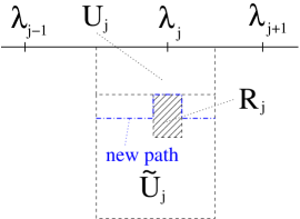
Figure 8. The new path

The count of the number of resonances given by the proof of Theorems 2.1 and 2.2 then shows that the equations (2.4) and (2.8) where $S_{L}$ and $\Gamma_{L}$ are respectively replaced by $S^{+}_{L}$ and $\Gamma^{+}_{L}$ have at most $C\ell_{L}$ solutions in the lower half plane. The equations where $S_{L}$ and $\Gamma_{L}$ are replaced by $S^{+}_{L}$ and $\Gamma^{+}_{L}$ we will call the $+$-equations. The analogue of Theorems 3.1, 3.2 and 3.3 for the $+$-equations and Theorem 6.2 show that the only solutions to the $+$-equations in the strip $\{$Re$\,E\in I,\ -e^{-4\ell_{L}/5}<$Im$\,E<-e^{-3\ell_{L}/4}\}$ are given by formulas (3.19) and (3.20) for the eigenvalues of the Dirichlet problem associated to a localization center in $\llbracket L-2\ell_{L},L-\ell_{L}/2\rrbracket$ if $\bullet=\mathbb{N}$ and in $\llbracket\ell_{L}/2,2\ell_{L}\rrbracket\cup\llbracket L-2\ell_{L},L-\ell_{L}/2\rrbracket$ if $\bullet=\mathbb{Z}$. Thus, these zeros are simple and separated by a distance at least $L^{-4}$ from each other (recall (6.10)). Moreover, we can cover the interval $I$ by intervals of the type $[(\lambda_{j}+\lambda_{j-1})/2,(\lambda_{j}+\lambda_{j+1})/2]$, that is, one can write

(6.15) $$I\subset\bigcup_{j=j^{-}}^{j^{+}}\left[\frac{\lambda_{j}+\lambda_{j-1}}{2},\frac{\lambda_{j}+\lambda_{j+1}}{2}\right]$$

where $\lambda_{j^{-}-1}\not\in I$, $\lambda_{1+j^{+}}\not\in I$, $\lambda_{j^{-}}\in I$ and $\lambda_{j^{+}}\in I$. Consider now the line $\{$Im$\,E=-e^{-\ell_{L}}\}$ and its intersection with the vertical strip $[(\lambda_{j}+\lambda_{j-1})/2,(\lambda_{j}+\lambda_{j+1})/2]-i\mathbb{R}^{+}$. Three things may occur:

1. either $e^{-\ell_{L}}<a_{j}dj^{2}|\sin\theta(\lambda_{j})|/C$ (the constant $C$ is defined in Theorem 3.1), then, on the interval $[(\lambda_{j}+\lambda_{j-1})/2,(\lambda_{j}+\lambda_{j+1})/2]-ie^{-\ell_{L}}$, one has

   (6.16) $$\left|S^{+}_{L}(E)+e^{-i\theta(E)}\right|\gtrsim 1\quad\text{ and }\quad\displaystyle\left|\text{det}\left(\Gamma^{+}_{L}(E)+e^{-i\theta(E)}\right)\right|\gtrsim 1;$$

   this follows from the proof of Theorem 3.1 (see in particular (3.5), (3.6), (3.7) and (3.8)) for some fixed $c>0$; recall that, on the interval $I+ie^{-\ell_{L}}$, one has $|\sin\theta(E)|\gtrsim 1$;

2. either $e^{-\ell_{L}}>Ca_{j}$ (the constant $C$ is defined in Theorem 3.2), then, on the interval $[(\lambda_{j}+\lambda_{j-1})/2,(\lambda_{j}+\lambda_{j+1})/2]-ie^{-\ell_{L}}$, one has again (6.16) for a possibly different constant; this follows from the proof of Theorem 3.2 (see in particular (3.15) and (3.16));

3. if we are neither in case (1) nor in case (2), then the line $\{$Im$\,E=-e^{-\ell_{L}}\}$ may cross $R_{j}$ (defined in Theorem 3.3; see also Fig. 7); we change the contour $\{$Im$\,E=-e^{-\ell_{L}}\}$ so as to enter $\tilde{U}_{j}$ until we reach the boundary of $R_{j}$ and then follow this boundary getting closer to the real axis, turning around $R_{j}$ and finally reaching the line $\{$Im$\,E=-e^{-\ell_{L}}\}$ again on the other side of $R_{j}$ and following it up to the boundary of $\tilde{U}_{j}$ (see Figure 8); on this new line, the bound (6.16) again holds; moreover, this new line is closer to the real axis than the line $\{$Im$\,E=-e^{-\ell_{L}}\}$.

Let us call $\mathcal{C}_{\ell}$ the path obtained by gluing together the paths constructed in points (1)-(3) for $j^{-}\leq j\leq j^{+}$ and the half-lines $\frac{\lambda_{j^{-}}+\lambda_{j^{-}-1}}{2}-i[e^{-\ell_{L}},+\infty)$ and $\frac{\lambda_{j^{+}}+\lambda_{j^{+}+1}}{2}-i[e^{-\ell_{L}},+\infty)$ (see (6.15)). One can then apply Rouché’s Theorem to compare the $+$ equations to the equations (2.4) and (2.8): by (6.14) and (6.16), on the line $\mathcal{C}_{\ell}$, one has $\displaystyle\left|S_{L}^{-}\right|<\left|S_{L}^{+}+e^{-i\theta}\right|$ and

$$\left|\text{det}\left(\Gamma_{L}(E)+e^{-i\theta(E)}\right)\text{det}\left(\Gamma^{+}_{L}(E)+e^{-i\theta(E)}\right)\right|\leq\frac{1}{2}\left|\text{det}\left(\Gamma_{L}(E)+e^{-i\theta(E)}\right)\right|.$$

Thus, the number of solutions to equations (2.4) and (2.8) below the line $\mathcal{C}_{\ell}$ is bounded by $C\ell_{L}$; as $\mathcal{C}_{\ell}$ lies above $\{$Im$\,E=-e^{-\ell_{L}}\}$, in the half-plane $\{$Im$\,E<-e^{-\ell_{L}}\}$, the equations (2.4) and (2.8) have at most $C\ell_{L}$ solutions. We have proved Theorem 1.10.∎

6.2.6. The proof of Theorem 1.11

The first point in Theorem 1.11 is proved in the same way as point (2) in Theorem 1.7 up to the change of scales, $L$ being replaced by $\ell_{L}$. Pick scales $(\ell^{\prime}_{L})_{L}$ satisfying (1.22) such that $\ell^{\prime}_{L}\ll\ell_{L}$. One has

Lemma 6.4.

Fix two sequences $(a_{L})_{L}$ and $(b_{L})_{L}$ such that $a_{L}<b_{L}$. With probability one, for $L$ sufficiently large,

$$\#\left\{\text{e.v. of }H_{\omega,\ell_{L}-2\ell^{\prime}_{L}/\rho}\text{ in }\left[a_{L}+e^{-\ell^{\prime}_{L}},b_{L}-e^{-\ell^{\prime}_{L}}\right]\right\}\\ \leq\#\left\{\text{e.v. of }H_{\omega,L}\text{ in }[a_{L},b_{L}]\text{ with loc. cent. in }\llbracket 0,\ell_{L}\rrbracket\right\}\\ \leq\#\left\{\text{e.v. of }H_{\omega,\ell_{L}+2\ell^{\prime}_{L}/\rho}\text{ in }\left[a_{L}-e^{-\ell^{\prime}_{L}},b_{L}+e^{-\ell^{\prime}_{L}}\right]\right\}$$

where $\rho$ is given by Lemma 6.1.

Proof.

To prove Lemma 6.4, we apply Lemma 6.1 to $L=\ell_{L}+\ell^{\prime}_{L}$ (i.e. for the operator $H_{\omega}$ restricted to the interval $\llbracket 0,\ell_{L}+\ell^{\prime}_{L}\rrbracket$) and $l_{L}=\ell^{\prime}_{L}$. The probability of the bad set is the $O\left(L^{-\infty}\right)$, thus, summable in $L$. Using the localization estimate (6.3), one proves that

• each eigenvalue of $H_{\omega,\ell_{L}-2\ell^{\prime}_{L}/\rho}$ is at a distance of at most $e^{-\ell^{\prime}_{L}}$ of an eigenvalue of $H_{\omega,L}$ with loc. cent. in $\llbracket 0,\ell_{L}\rrbracket$;

• each eigenvalue of $H_{\omega,L}$ with loc. cent. in $\llbracket 0,\ell_{L}\rrbracket$ is at a distance of at most $e^{-\ell^{\prime}_{L}}$ of an eigenvalue of $H_{\omega,\ell_{L}+2\ell^{\prime}_{L}/\rho}$.

Lemma 6.4 follows. ∎

The first point in Theorem 1.11 is then point (2) of Theorem 1.7 for the operator $H_{\omega,\ell_{L}-2\ell^{\prime}_{L}/\rho}$ and $H_{\omega,\ell_{L}+2\ell^{\prime}_{L}/\rho}$ and the fact that $\ell^{\prime}_{L}\ll\ell_{L}$.The proof of the second statement in Theorem 1.11 is very similar to that of Theorem 1.8. Fix $I$ a compact interval in $\overset{\circ}{\Sigma}$. As $\ell_{L}$ satisfies (1.22), one can find $\ell^{\prime}_{L}<\ell^{\prime\prime}_{L}$ also satisfying (1.22) such that $\displaystyle e^{-\ell^{\prime\prime}_{L}}\ll e^{-\ell_{L}}\ll e^{-\ell^{\prime}_{L}}$. For the same reasons as in the proof of Theorem 1.8, after rescaling, all the resonances in $\displaystyle I-i(-\infty,0)$ outside the strip $\displaystyle I-i\left[e^{-\ell^{\prime}_{L}},e^{-\ell^{\prime\prime}_{L}}\right)$ are then pushed to either $0$ or $i\infty$ as $L\to+\infty$.
On the other hand, the resonances in the strip $\displaystyle I-i\left[e^{-\ell^{\prime}_{L}},e^{-\ell^{\prime\prime}_{L}}\right)$ are described by (3.19). The rescaled real and imaginary parts of the resonances (see (1.24)) now become $x_{j}=(E_{j,\omega}-E)\ell_{L}+o(1)$ and $y_{j}=\rho(E)\frac{d_{j,\omega}}{\ell_{L}}+o(1)$.
Now, to compute the limit of $\mathbb{P}(\#\{j;\ x_{j}\in I,\ y_{j}\in J\}=k)$, using the exponential decay property (6.3), it suffices to use [13, Theorem 1.14]. Let us note here that [13, condition (1.50)] on the scales $(\ell_{L})_{L}$ is slightly stronger than (1.22). That condition (1.22) suffices is a consequence of the stronger localization property known in the present case (compare Theorem 6.2 to [13, Assumption (Loc)]). This completes the proof of the second point in Theorem 1.11. The final statement in 1.11 is proved in exactly the same way as Theorem 1.9.
The proof of Theorem 1.11 is complete.∎

6.2.7. The proofs of Proposition 1.3 and Theorem 1.12

Localization for the operator $H^{\mathbb{N}}_{\omega}$ can be described by the following

Lemma 6.5.

There exists $\rho>0$ and $q>0$ such that, $\omega$ almost surely, there exists $C_{\omega}>0$ s.t. for $L$ sufficiently large, if

1. $\varphi_{j,\omega}$ is a normalized eigenvector of $H_{\omega,L}$ associated to $E_{j,\omega}$ in $\Sigma$,

2. $x_{j}(\omega)\in\mathbb{N}$ is a maximum of $x\mapsto|\varphi_{j,\omega}(x)|$ in $\mathbb{N}$,

then, for $x\in\mathbb{N}$, one has

(6.17) $$|\varphi_{j,\omega}(x)|\leq C_{\omega}(1+|x_{j}(\omega)|^{2})^{q/2}e^{-\rho|x-x_{j}(\omega)|}.$$

Moreover, the mapping $\omega\mapsto C_{\omega}$ is measurable and $\mathbb{E}(C_{\omega})<+\infty$.

This result for our model is a consequence of Theorem 6.1 (see, e.g., [28, 10, 7]) and [13, Theorem 6.1].
We thus obtain the following representation for the function $\Xi_{\omega}$

(6.18) $$\Xi_{\omega}(E)=\sum_{j}\frac{|\varphi_{j,\omega}(0)|^{2}}{E_{j,\omega}-E}+e^{-i\arccos(E/2)}$$

As $H_{\omega}^{\mathbb{N}}$ satisfies a Dirichlet boundary condition at $-1$, one has

(6.19) $$\forall j,\quad|\varphi_{j,\omega}(0)|>0\quad\text{and}\quad\sum_{j}|\varphi_{j,\omega}(0)|^{2}=1.$$

As $E\to-i\infty$, the representation (6.18) yields

$$\begin{split}\Xi_{\omega}(E)&=-E^{-2}\sum_{j}|\varphi_{j,\omega}(0)|^{2}E_{j,\omega}+O\left(E^{-3}\right)=-E^{-2}\langle\delta_{0},H_{\omega}^{\mathbb{N}}\delta_{0}\rangle+O\left(E^{-3}\right)\\ &=-\omega_{0}\,E^{-2}+O\left(E^{-3}\right).\end{split}$$

This proves the first point in Proposition 1.3.
As a direct consequence of Theorem 6.1 and the computation leading to Theorem 5.2 (see section 5.1.2), we obtain that there exists $\tilde{c}>0$ s.t. for $L$ sufficiently large, with probability at least $1-e^{-\tilde{c}L}$, one has

(6.20) $$\sup_{\text{Im}\,E\leq-e^{-\tilde{c}L}}\left|\int_{\mathbb{R}}\frac{dN_{\omega}(\lambda)}{\lambda-E}-\langle\delta_{0},(H_{\omega,L}-E)^{-1}\delta_{0}\rangle\right|\leq e^{-\tilde{c}L}.$$

Taking

(6.21) $$L=L_{\varepsilon}\sim c^{-1}|\log\varepsilon|$$

for some sufficiently small $c>0$, this and Rouché’s Theorem implies that, with probability $1-\varepsilon^{3}$, the number of zeros of $\Xi_{\omega}$ (counted with multiplicity) in $I+i(-\infty,\varepsilon]$ is bounded

• from above by the number of resonances of $H_{\omega,L_{\varepsilon}}$ in $I_{\varepsilon}^{+}+i(-\infty,-\varepsilon-\varepsilon^{2}]$;

• from below by the number of resonances of $H_{\omega,L_{\varepsilon}}$ in $I_{\varepsilon}^{-}+i(-\infty,-\varepsilon+\varepsilon^{2}]$.

where $I_{\varepsilon}^{+}=[a-\varepsilon,b+\varepsilon]$ and $I_{\varepsilon}^{+}=[a+\varepsilon,b-\varepsilon]$ if $I=[a,b]$.
Here, to apply Rouché’s Theorem, we apply the same strategy as in the proof of Theorem 1.10 and construct a path bounding a region larger (resp. smaller) than $I_{\varepsilon}^{+}+i(-\infty,-\varepsilon-\varepsilon^{2}]$ (resp. $I_{\varepsilon}^{-}+i(-\infty,-\varepsilon+\varepsilon^{2}]$) on which one can guarantee $\displaystyle\left|S_{L}(E)+e^{-i\theta(E)}\right|\gtrsim 1$.
Now, we choose the constant $c$ (see (6.21)) to be so small that $\displaystyle c<\min_{E\in I}\rho(E)$. Applying point (3) of Theorem 1.7 to $H_{\omega,L_{\varepsilon}}$ with this constant $c$, we obtain that the number of resonances of $H_{\omega,L_{\varepsilon}}$ in $I_{\varepsilon}^{+}+i(-\infty,\varepsilon-\varepsilon^{2}]$ (resp. $I_{\varepsilon}^{-}+i(-\infty,\varepsilon+\varepsilon^{2}]$) is upper bounded (resp lower bounded) by

$$\begin{split}L_{\varepsilon}\int_{I}\min\left(\frac{c}{\rho(E)},1\right)n(E)dE\,(1+O(1))&=\frac{|\log\varepsilon|}{c}\int_{I}\frac{c}{\rho(E)}n(E)dE\,(1+O(1))\\ =&|\log\varepsilon|\int_{I}\frac{n(E)}{\rho(E)}dE\,(1+O(1)).\end{split}$$

Hence, we obtain the second point of Proposition 1.3. The last point of this proposition is then an immediate consequence of the arguments developed to obtain the second point if one takes into account the following facts:

• the minimal distance between the Dirichlet eigenvalues of $H^{\mathbb{N}}_{\omega,L}$ is bounded from below by $L^{-4}$ (see (6.10)),

• the growth of the function $E\mapsto S_{L}(E)+e^{-i\theta(E)}$ near the resonances (i.e. its zeros) is well controlled by Proposition 3.1.

Indeed, this implies that the resonances of $H^{\mathbb{N}}_{\omega,L}$ are simple in $I+i[-e^{-\sqrt{L}},0)$ (one can choose larger rectangles) and that near each resonance one can apply Rouché’s Theorem to control the zero of $\Xi_{\omega}$. Note that this also yields $\omega$-almost surely, there exists $c_{\omega}$ such that

(6.22) $$\min_{\begin{subarray}{c}z\text{ zero of }\Xi_{\omega}\\ z\in I+i(-\varepsilon_{\omega},0)\end{subarray}}\inf_{0<r<\varepsilon_{\omega}(\text{Im}\,z)^{3/2}}\min_{|E-z|=r}\frac{|\Xi_{\omega}(E)|}{r}\gtrsim 1.$$

This completes the proof of Proposition 1.3.∎Theorem 1.12 is a consequence of the following

Theorem 6.4.

There exists $\tilde{c}>0$ such that, $\omega$ almost surely, for $L\geq 1$ sufficiently large one has

$$\sup_{\begin{subarray}{c}\text{Re}\,E\in I\\ \text{Im}\,E<-e^{-\tilde{c}L}\end{subarray}}\left|\Gamma_{L,\omega,\tilde{\omega}}(E)-\begin{pmatrix}\displaystyle\int_{\mathbb{R}}\frac{dN_{\tilde{\omega}}(\lambda)}{\lambda-E}&0\\ 0&\displaystyle\int_{\mathbb{R}}\frac{dN_{\omega}(\lambda)}{\lambda-E}\end{pmatrix}\right|+\left|S_{L,\omega}(E)-\int_{\mathbb{R}}\frac{dN_{\omega}(\lambda)}{\lambda-E}\right|\leq e^{-\tilde{c}L}$$

where $\Gamma_{L,\omega,\tilde{\omega}}(E)$ (resp. $S_{L,\omega}(E)$) is the matrix $\Gamma_{L}(E)$ (resp. the function $S_{L}(E)$) (see (2.9)) constructed from the Dirichlet data on $\llbracket 0,L\rrbracket$ of $-\Delta+V^{\mathbb{Z}}_{\omega,\tilde{\omega},L}$ (resp. $-\Delta+V^{\mathbb{N}}_{\omega,L}$) (see (1.26)) using formula (2.9) (resp. (2.4)).

Theorem 6.4 is proved exactly as Theorem 5.2 except that one uses the localization estimates (6.2) instead of the Combes-Thomas estimates.
Theorem 1.12 is then an immediate consequence of the estimate (6.20). Indeed, this implies that if $z$ is a resonance for e.g. $H^{N}_{\omega,L}$ in $\displaystyle I+i\left(-\infty,e^{\tilde{c}L}\right]$, then $\displaystyle|\Xi_{\omega}(z)|\leq e^{-\tilde{c}L}$. By the last point of Proposition 1.3, $\omega$ almost surely, we know that the multiplicity of the zeros of $\Xi_{\omega}$ is bounded by $N_{\omega}$. Moreover, for the zeros of $\Xi_{\omega}$ in $I+i(-\varepsilon_{\omega},0)$, we know the bound (6.22). This bound and (6.20) imply that

$$\max_{\begin{subarray}{c}z\text{ zero of }\Xi_{\omega}\\ z\in I+i\left(-\varepsilon_{\omega},e^{-\tilde{c}L}\right)\end{subarray}}\max_{|E-z|=e^{-\tilde{c}L}}\frac{\left|\Xi_{\omega}(E)-\left(S_{\omega,L}(E)+e^{-i\theta(E)}\right)\right|}{\left|\Xi_{\omega}(E)\right|}<e^{-\tilde{c}L}.$$

This yields point (2) in Theorem 1.12 by an application of Rouché’s Theorem. Point (1) is obtained in the same way using Proposition 3.1 that gives

$$\max_{\begin{subarray}{c}z\text{ resonance of }H^{\mathbb{N}}_{\omega,L}\\ z\in I+i\left(-\varepsilon_{\omega},e^{-\tilde{c}L}\right)\end{subarray}}\max_{|E-z|=e^{-\tilde{c}L}}\frac{\left|\Xi_{\omega}(E)-\left(S_{\omega,L}(E)+e^{-i\theta(E)}\right)\right|}{\left|S_{\omega,L}(E)+e^{-i\theta(E)}\right|}<e^{-\tilde{c}L}.$$

The case of $H^{\mathbb{Z}}_{\omega,\tilde{\omega},L}$ is dealt with in the same way.
This completes the proof of Theorem 1.12.∎

6.3. Estimates on the growth of eigenfunctions

In the present section we are going to prove Theorems 6.2 and 6.3. At the end of the section, we also prove the simpler Lemma 6.2.
The proof of Theorem 6.2 relies on locally uniform estimates on the rate of growth of the cocycle (1.15) attached to the Schrödinger operator that we present now. Define

(6.23) $$T_{L}(E,\omega)=T(E,\omega_{L})\cdots T(E,\omega_{0})$$

where

$$T(E,\omega_{j})=\begin{pmatrix}E-\omega_{j}&-1\\ 1&0\end{pmatrix}$$

We start with an upper bound on the large deviations of the growth rate of the cocycle that is uniform in energy. Fix $\alpha>1$ and $\delta\in(0,1)$. For one part, the proof of Theorem 6.2 relies on the following

Lemma 6.6.

Let $I\subset\mathbb{R}$ be a compact interval. For any $\delta>0$, there exists $L_{\delta}>0$ and $\eta>0$ such that, for $L\geq L_{\delta}$ and any $K>0$, one has

(6.24) $$\mathbb{P}\left(\begin{aligned} &\forall 0\leq k\leq K,\quad\forall E\in I,\quad\forall\|u\|=1,\\ \ &\frac{\log\|T_{L}(E;\tau^{k}(\omega))u\|}{L+1}\leq\rho(E)+\delta\end{aligned}\right)\geq 1-Ke^{-\eta(L+1)}$$

where we recall that $\tau:\Omega\to\Omega$ denotes the left shift (i.e. if $\omega=(\omega_{n})_{n\geq 0}$ then $\displaystyle[\tau(\omega)]_{n}=\omega_{n+1}$ for $n\geq 0$) and $\tau^{n}=\tau\circ\cdots\circ\tau$ $n$ times.

At the heart of this result is a large deviation principle for the growth rate of the cocycle (see [5, section I and Theorem 6.1]). As it also serves in the proof of Theorem 6.2, we recall it now. One has

Lemma 6.7.

Let $I\subset\mathbb{R}$ be a compact interval. For any $\delta>0$, there exists $L_{\delta}>0$ and $\eta>0$ such that, for $L\geq L_{\delta}$, one has

(6.25) $$\sup_{\begin{subarray}{c}E\in I\\ \|u\|=1\end{subarray}}\mathbb{P}\left(\left|\frac{\log\|T_{L}(E;\omega)u\|}{L+1}-\rho(E)\right|\geq\delta\right)\leq e^{-\eta(L+1)}.$$

While this result is not stated as is in [5], it can be obtained from [5, Lemma 6.2 and Theorem 6.1]. Indeed, by inspecting the proof of [5, Lemma 6.2 and Theorem 6.1], it is clear that the quantities involved (in particular, the principal eigenvalue of $T(z;E)=T(z)$ in [5, Theorem 4.3]) are continuous functions of the energy $E$. Thus, taking this into account, the proof of [5, Theorem 6.1] yields, for our cocycle, a convergence that is locally uniform in energy, that is, (6.25). To prove Theorem 6.2, in addition to Lemma 6.6, we also need to guarantee a uniform lower bound on the growth rate of the cocycle. We need this bound at least on the spectrum of $H_{\omega,L}$ with a good probability. Actually, this is the best one can hope for: a uniform bound in the style of (6.24) will not hold.
We prove

Lemma 6.8.

Fix $I$ a compact interval and $\delta>0$. Pick $u\in\mathbb{C}^{2}$ s.t. $\|u\|=1$. For $0\leq j\leq L$, if $j\leq L-1$, define

$$\mathcal{K}^{+}_{j}(\omega,L,\delta,u):=\left\{E\in I;\ \left|\frac{\log\left\|T^{-1}_{L-(j+1)}(E,\tau^{j+1}(\omega))u\right\|}{L-j}-\rho(E)\right|>\delta\right\}$$

and, if $$1\leq j$$, define

$$\mathcal{K}^{-}_{j}(\omega,L,\delta,u):=\left\{E\in I;\ \left|\frac{\log\left\|T_{j-1}(E,\omega)u\right\|}{j}-\rho(E)\right|>\delta\right\};$$

finally, define $\mathcal{K}^{+}_{L}(\omega,L,\delta,u)=\emptyset=\mathcal{K}^{-}_{0}(\omega,L,\delta,u)$.
Recall that $(E_{j,\omega})_{0\leq j\leq L}$ are the eigenvalues of $H_{\omega,L}$ and let $x_{j,\omega}$ be the associated localization centers.
For $0\leq\ell\leq L$, define the sets

$$\Omega^{+}_{B}(L,\ell,\delta,u):=\left\{\omega;\begin{aligned} \exists j\text{ s.t. }L-x_{j,\omega}\geq\ell\text{ and }\\ E_{j,\omega}\in\mathcal{K}^{+}_{x_{j,\omega}}(\omega,L,\delta,u)\end{aligned}\right\}$$

and

$$\Omega^{-}_{B}(L,\ell,\delta,u):=\left\{\omega;\begin{aligned} \exists j\text{ s.t. }x_{j,\omega}\geq\ell\text{ and }\\ E_{j,\omega}\in\mathcal{K}^{-}_{x_{j,\omega}}(\omega,L,\delta,u)\end{aligned}\right\}.$$

Then, the sets $\Omega^{\pm}_{B}(L,\ell,\delta,u)$ are measurable and, for any $\delta>0$, there exists $\eta>0$ and $\ell_{0}>0$ such that, for $L\geq\ell\geq\ell_{0}$, one has

(6.26) $$\max\left(\mathbb{P}(\Omega^{+}_{B}(L,\ell,\delta,u)),\mathbb{P}(\Omega^{-}_{B}(L,\ell,\delta,u))\right)\leq\frac{(L+1)|I|e^{-\eta(\ell-1)}}{1-e^{-\eta}}.$$

Here, the constant $\eta$ is the one given by (6.25).

First, let us explain the meaning of Lemma 6.8. As, by Lemma 6.6, we already control the growth of the cocycle from above, we see that in the definitions of the set $\mathcal{K}^{-}_{j}(\omega,L,\delta,u)$ resp. $\mathcal{K}^{+}_{j}(\omega,L,\delta,u)$, it would have sufficed to require

$$\frac{\log\left\|T_{j-1}(E,\omega)u\right\|}{j}-\rho(E)\leq-\delta$$

resp.

$$\frac{\log\left\|T^{-1}_{L-(j+1)}(E,\tau^{j+1}(\omega))u\right\|}{L-(j+1)}-\rho(E)\leq-\delta.$$

Hence, what Lemma 6.8 measures is that the probability that the cocycle at energy $E_{n,\omega}$ leading from a localization center $x_{n,\omega}$ to either $0$ or $L$ decays at a rate smaller than the rate predicted by the Lyapunov exponent.
The sets $\Omega^{\pm}_{B}(L,\ell,\delta,u)$ are the sets of bad configurations, i.e., the events when the rate of decay of the solution is far from the Lyapunov exponent. Indeed, for $\omega$ outside $\Omega^{\pm}_{B}(L,\ell,\delta)$, i.e., if the reverse of the inequalities defining $\mathcal{K}^{\pm}_{j}(\omega,L,\delta,u)$ hold, when $j=x_{n,\omega}$ and $E=E_{n,\omega}$, then, we know that the eigenfunction $\varphi_{n,\omega}$ has to decay from the center of localization $x_{n,\omega}$ (which is a local maximum of its modulus) towards the edges of the intervals at a rate larger than $\gamma(E_{n,\omega})-\delta$. The eigenfunction being normalized, at the localization center, it is of size at least $L^{-1/2}$. This will entail the estimates (6.4) and (6.5) with a good probability. There is a major difference in the uniformity in energy obtained in Lemmas 6.8 and 6.6. In Lemma 6.8, we do not get a lower bound on the decay rate that is uniform all over $I$: it is merely uniform over the spectrum inside $I$ (which is sufficient for our purpose as we shall see). The reason for this difference in the uniformity between Lemma 6.6 and 6.8 is the same that makes the Lyapunov exponent $E\mapsto\rho(E)$ in general only upper semi-continuous and not lower semi-continuous (in the present situation, it actually is continuous). We postpone the proofs of Lemmas 6.6 and 6.8 to the end of this section and turn to the proofs of Theorems 6.2 and 6.3.

6.3.1. The proof of Theorem 6.2

By Lemma 6.6, as $T_{L}(E,\omega)\in SL(2,\mathbb{R})$, with probability at least $1-KLe^{-\eta(L+1)}$, for $L\geq L_{\delta}$ and any $K>0$, one also has

$$\forall 0\leq k\leq K,\quad\forall E\in I,\quad\forall\|u\|=1,\quad\frac{\log\|T^{-1}_{L}(E;\tau^{k}(\omega))u\|}{L+1}\leq\rho(E)+\delta.$$

Now pick $\ell=C\log L$ where $C>0$ is to be chosen later on. We know that, with probability $\mathbb{P}$ satisfying

(6.27) $$\mathbb{P}\geq 1-L^{2}e^{-\eta\ell},$$

for $L\geq L_{\delta}$ and any $l\in[\ell,L]$ and any $k\in[0,L]$, one also has

(6.28) $$\forall E\in I,\quad\forall\|u\|=1,\quad\frac{\log\|T^{-1}_{l}(E;\tau^{k}(\omega))u\|}{l+1}\leq\rho(E)+\delta.$$

Let $\varphi_{j,\omega}$ be a normalized eigenfunction associated to the eigenvalue $E_{j,\omega}\in I$ with localization center $x_{j,\omega}$. By the definition of the localization center, one has

(6.29) $$\frac{1}{L+1}\leq\left\|\begin{pmatrix}\varphi_{j,\omega}(x_{j,\omega})\\ \varphi_{j,\omega}(x_{j,\omega}-1)\end{pmatrix}\right\|^{2}\leq 1\quad\text{and}\quad\frac{1}{L+1}\leq\left\|\begin{pmatrix}\varphi_{j,\omega}(x_{j,\omega}+1)\\ \varphi_{j,\omega}(x_{j,\omega})\end{pmatrix}\right\|^{2}\leq 1.$$

By the eigenvalue equation, for $x\in\llbracket 0,L\rrbracket$, one has

(6.30) $$\begin{pmatrix}\varphi_{j,\omega}(x)\\ \varphi_{j,\omega}(x-1)\end{pmatrix}=\begin{cases}T_{x-x_{j,\omega}}(E;\tau^{x_{j,\omega}}(\omega))\begin{pmatrix}\varphi_{j,\omega}(x_{j,\omega})\\ \varphi_{j,\omega}(x_{j,\omega}-1)\end{pmatrix}&\text{ if }x\geq x_{j,\omega},\\ T^{-1}_{x_{j,\omega}-x}(E;\tau^{x}(\omega))\begin{pmatrix}\varphi_{j,\omega}(x_{j,\omega})\\ \varphi_{j,\omega}(x_{j,\omega}-1)\end{pmatrix}&\text{ if }x\leq x_{j,\omega}.\end{cases}$$

Hence, by (6.24) and (6.28), with probability at least $1-2L^{2}e^{-\eta\ell}-L^{-p}$, if $|x_{j,\omega}-x|\geq\ell$, for $x_{j,\omega}<x\leq L$, one has

(6.31) $$\begin{split}\frac{e^{-(\rho(E_{j,\omega})+\delta)|x-x_{j,\omega}|}}{\sqrt{L+1}}&\leq e^{-(\rho(E_{j,\omega})+\delta)|x-x_{j,\omega}|}\left\|\begin{pmatrix}\varphi_{j,\omega}(x_{j,\omega})\\ \varphi_{j,\omega}(x_{j,\omega}-1)\end{pmatrix}\right\|\\ &\leq\left\|T_{x-x_{j,\omega}}(E;\tau^{x_{j,\omega}}(\omega))\begin{pmatrix}\varphi_{j,\omega}(x_{j,\omega})\\ \varphi_{j,\omega}(x_{j,\omega}-1)\end{pmatrix}\right\|=\left\|\begin{pmatrix}\varphi_{j,\omega}(x)\\ \varphi_{j,\omega}(x-1)\end{pmatrix}\right\|\end{split}$$

and, for $0\leq x<x_{j,\omega}$, one has

(6.32) $$\begin{split}\left\|\begin{pmatrix}\varphi_{j,\omega}(x)\\ \varphi_{j,\omega}(x-1)\end{pmatrix}\right\|&=\left\|T^{-1}_{x-x_{j,\omega}}(E;\tau^{x_{j,\omega}}(\omega))\begin{pmatrix}\varphi_{j,\omega}(x_{j,\omega})\\ \varphi_{j,\omega}(x_{j,\omega}-1)\end{pmatrix}\right\|\\ &\geq e^{-(\rho(E_{j,\omega})+\delta)|x-x_{j,\omega}|}\left\|\begin{pmatrix}\varphi_{j,\omega}(x_{j,\omega})\\ \varphi_{j,\omega}(x_{j,\omega}-1)\end{pmatrix}\right\|\geq\frac{e^{-(\rho(E_{j,\omega})+\delta)|x-x_{j,\omega}|}}{\sqrt{L+1}}\end{split}$$

On the other hand, by the definition of the Dirichlet boundary conditions, we know that

$$\begin{pmatrix}\varphi_{j,\omega}(0)\\ \varphi_{j,\omega}(-1)\end{pmatrix}=\varphi_{j,\omega}(0)\begin{pmatrix}1\\ 0\end{pmatrix}\quad\text{and}\quad\begin{pmatrix}\varphi_{j,\omega}(L+1)\\ \varphi_{j,\omega}(L)\end{pmatrix}=\varphi_{j,\omega}(L)\begin{pmatrix}0\\ 1\end{pmatrix}.$$

Thus,

$$\varphi_{j,\omega}(0)\,T_{x_{j,\omega}-1}(E;\omega)\begin{pmatrix}1\\ 0\end{pmatrix}=\begin{pmatrix}\varphi_{j,\omega}(x_{j,\omega})\\ \varphi_{j,\omega}(x_{j,\omega}-1)\end{pmatrix}$$

and

$$\varphi_{j,\omega}(L)\begin{pmatrix}0\\ 1\end{pmatrix}=T_{L-x_{j,\omega}-1}(E;\tau^{x_{j,\omega}+1}(\omega))\begin{pmatrix}\varphi_{j,\omega}(x_{j,\omega}+1)\\ \varphi_{j,\omega}(x_{j,\omega})\end{pmatrix}.$$

Thus, for $\omega\not\in\Omega^{+}_{B}(L,\ell,\delta,u_{+})\cup\Omega^{-}_{B}(L,\ell,\delta,u_{-})$ where we have set $\displaystyle u_{-}:=\begin{pmatrix}0\\ 1\end{pmatrix}$ and $\displaystyle u_{+}:=\begin{pmatrix}1\\ 0\end{pmatrix}$, we know that

$$e^{-(\rho(E_{j,\omega})-\delta)(L-x_{j,\omega})}\leq\left\|T^{-1}_{L-x_{j,\omega}-1}(E;\tau^{x_{j,\omega}+1}(\omega))u_{+}\right\|$$

and

$$e^{-(\rho(E_{j,\omega})-\delta)x_{j,\omega}}\leq\left\|T_{x_{j,\omega}-1}(E;\omega)u_{-}\right\|$$

Thus, we obtain that, for $\omega\not\in\Omega^{+}_{B}(L,\ell,\delta,u_{+})\cup\Omega^{-}_{B}(L,\ell,\delta,u_{-})$, one has

(6.33) $$\begin{split}|\varphi_{j,\omega}(L)|&=\left\|T^{-1}_{L-x_{j,\omega}}(E;\tau^{x_{j,\omega}+1}(\omega))\begin{pmatrix}0\\ 1\end{pmatrix}\right\|^{-1}\left\|\begin{pmatrix}\varphi_{j,\omega}(x_{j,\omega}+1)\\ \varphi_{j,\omega}(x_{j,\omega})\end{pmatrix}\right\|\\ &\leq e^{-(\rho(E_{j,\omega})-\delta)(L-x_{j,\omega}-1)}\end{split}$$

and

(6.34) $$\begin{split}|\varphi_{j,\omega}(0)|&=\left\|T_{x_{j,\omega}}(E;\tau^{x_{j,\omega}}(\omega))\begin{pmatrix}0\\ 1\end{pmatrix}\right\|^{-1}\left\|\begin{pmatrix}\varphi_{j,\omega}(x_{j,\omega})\\ \varphi_{j,\omega}(x_{j,\omega}-1)\end{pmatrix}\right\|\\ &\leq e^{-(\rho(E_{j,\omega})-\delta)(x_{j,\omega}-1)}.\end{split}$$

The estimates given by Lemma 6.8 on the probability of $\Omega^{+}_{B}(L,\ell,\delta,u_{+})$ and $\Omega^{-}_{B}(L,\ell,\delta,u_{-})$ for $\ell=C\log L$ and the estimate (6.27) then imply that, with a probability at least $1-4L^{2}e^{-\eta(\ell-1)}-L^{-p}$, the bounds (6.31), (6.32), (6.33) and (6.34) hold. Thus, picking $\ell=C\log L$ for $C>0$ sufficiently large (depending only on $\eta$, thus, on $\delta$ and $p$), these bounds hold with a probability at least $1-L^{-p}$. This complete the proof of Theorem 6.2.∎

Remark 6.1.

One may wonder whether the uniform growth estimate given by Lemmas 6.6 and 6.8 is actually necessary in the proof of Theorem 6.2. That they are necessary is due to the fact that both the eigenvalue $E_{j,\omega}$ and the localization center $x_{j,\omega}$ (and, thus, the vector $\displaystyle\left\|\begin{pmatrix}\varphi_{j,\omega}(x_{j,\omega})\\ \varphi_{j,\omega}(x_{j,\omega}-1)\end{pmatrix}\right\|$) depend on $\omega$. Thus, (6.25) is not sufficient to estimate the second term in the left hand sides of (6.31) and (6.32).

6.3.2. The proof of Theorem 6.3

To prove Theorem 6.3, we follow the strategy that led to the proof of Theorem 6.2. First, note that (6.31) and (6.32) provide the expected lower bounds on the eigenfunction with the right probability. As for the upper bound, by (6.30), using the conclusions of Theorem 6.2 and the bounds given by Lemma 6.6, we know that, e.g. for $0\leq x<x_{j,\omega}$

$$\begin{split}\left\|\begin{pmatrix}\varphi_{j,\omega}(x)\\ \varphi_{j,\omega}(x-1)\end{pmatrix}\right\|&=\left\|T_{x}(E;\omega)\begin{pmatrix}1\\ 0\end{pmatrix}\right\||\varphi_{j,\omega}(0)|\leq e^{(\rho(E_{j,\omega})+\delta)x}e^{-(\rho(E_{j,\omega})-\delta)x_{j,\omega}}\\ &\leq e^{-(\rho(E_{j,\omega})-C\delta)|x-x_{j,\omega}|}\end{split}$$

if $(1+C)x\leq(C-1)x_{j,\omega}$, i.e., $2(1+C)^{-1}x_{j,\omega}\leq x_{j,\omega}-x$.
For $x\geq x_{j,\omega}$ one reasons similarly and, thus, completes the proof of Theorem 6.3.∎

Remark 6.2.

Actually, as the proof shows, the results one obtains are more precise than the claims made in Theorem 6.3 (see [24]).

6.3.3. The proof of Lemma 6.8

The proofs for the two sets $\Omega^{\pm}_{B}(L,\ell,\delta,u)$ are the same. We will only write out the one for $\Omega^{+}_{B}(L,\ell,\delta,u)$. Let us first address the measurability issue for $\Omega^{+}_{B}(L,\ell,\delta,u)$. The functions $\omega\mapsto E_{j,\omega}$ and $\omega\mapsto\varphi_{j,\omega}$ are continuous (as the eigenvalues and eigenvectors of finite dimensional matrices depending continuously on the parameter $\omega=(\omega_{j})_{0\leq j\leq L}$). Thus, for fixed $j$, the sets $\{\omega;\ E_{j,\omega}\in\mathcal{K}^{-}_{j}(\omega,L,\delta,u)\}$ and $\{\omega;\ x_{j,\omega}>j\}$ are open (we used the definition of $x_{j,\omega}$ as the left most localization center (see Theorem 6.2)). This yields the measurability of $\Omega^{+}_{B}(L,\ell,\delta,u)$. We claim that

(6.35) $$\frac{1}{L+1}\mathbf{1}_{\Omega^{+}_{B}(L,\ell,\delta,u)}\leq\sum_{j=0}^{L+1-\ell}\langle\delta_{j},\mathbf{1}_{\mathcal{K}^{+}_{j}(\omega,L,\delta,u)}(H_{\omega,L})\delta_{j}\rangle$$

where $\mathbf{1}_{\mathcal{K}^{+}_{j}(\omega,L,\delta,u)}(H_{\omega,L})$ denotes the spectral projector associated to $H_{\omega,L}$ on the set $\mathcal{K}^{+}_{j}(\omega,L,\delta,u)$. Indeed, if one has $E_{j,\omega}\not\in\mathcal{K}^{+}_{x_{j,\omega}}(\omega,L,\delta,u)$ for all $j$ then the left hand side of (6.35) vanishes and the right hand side is non negative. On the other hand, if, for some $j$, one has $0\leq x_{j,\omega}\leq L-\ell$ and $E_{j,\omega}\in\mathcal{K}^{+}_{x_{j,\omega}}(\omega,L,\delta,u)$ then, we compute

$$\begin{split}\sum_{l=0}^{L-\ell}\langle\delta_{l},\mathbf{1}_{\mathcal{K}^{+}_{j}(\omega,L,\delta,u)}(H_{\omega,L})\delta_{l}\rangle&=\sum_{l=0}^{L-\ell}\sum_{\begin{subarray}{c}k\text{ s.t}\\ E_{k,\omega}\in\mathcal{K}^{+}_{j}(\omega,L,\delta,u)\end{subarray}}|\varphi_{k,\omega}(l)|^{2}\geq|\varphi_{j,\omega}(x_{j,\omega})|^{2}\\ &\geq\frac{1}{L+1}\geq\frac{1}{L+1}\mathbf{1}_{\Omega^{+}_{B}(L,\ell,\delta,u)}\end{split}$$

by the definition of $x_{j,\omega}$.
An important fact is that, by construction (see Lemma 6.8), the set of energies $\mathcal{K}^{+}_{j}(\omega,L,\delta,u)$ does not depend on $\omega_{j}$. Hence, denoting by $\mathbb{E}_{\omega_{j}}(\cdot)$ the expectation with respect to $\omega_{j}$ and $\mathbb{E}_{\hat{\omega}_{j}}(\cdot)$ the expectation with respect to $\hat{\omega}_{j}=(\omega_{k})_{k\not=j}$, we compute

$$\mathbb{E}\left(\sum_{j=0}^{L-\ell}\langle\delta_{j},\mathbf{1}_{\mathcal{K}^{+}_{j}(\omega,L,\delta,u)}(H_{\omega,L})\delta_{j}\rangle\right)=\sum_{j=0}^{L-\ell}\mathbb{E}_{\hat{\omega}_{j}}\left(\mathbb{E}_{\omega_{j}}\left(\langle\delta_{j},\mathbf{1}_{\mathcal{K}^{+}_{j}(\omega,L,\delta,u)}(H_{\omega,L})\delta_{j}\rangle\right)\right)$$

As $\omega_{j}$ is assumed to have a bounded compactly supported distribution and as $\mathcal{K}^{+}_{j}(\omega,L,\delta,u)$ does not depend on $\omega_{j}$, a standard spectral averaging lemma (see, e.g., [37, Theorem 11.8]) yields

$$\mathbb{E}_{\omega_{j}}\left(\langle\delta_{j},\mathbf{1}_{\mathcal{K}^{+}_{j}(\omega,L,\delta,u)}(H_{\omega,L})\delta_{j}\rangle\right)\leq|\mathcal{K}^{+}_{j}(\omega,L,\delta,u)|$$

where $|\cdot|$ denotes the Lebesgue measure. Thus, we obtain

(6.36) $$\mathbb{E}\left(\sum_{j=0}^{L-\ell}\langle\delta_{j},\mathbf{1}_{\mathcal{K}^{+}_{j}(\omega,L,\delta,u)}(H_{\omega,L})\delta_{j}\rangle\right)\leq\sum_{j=0}^{L-\ell}\mathbb{E}_{\hat{\omega}_{j}}\left(|\mathcal{K}^{+}_{j}(\omega,L,\delta,u)|\right)\\ =\sum_{j=0}^{L-\ell}\mathbb{E}\left(|\mathcal{K}^{+}_{j}(\omega,L,\delta,u)|\right).$$

By Lemma 6.7 and the Fubini-Tonelli theorem, we know that

$$\begin{split}\mathbb{E}\left(|\mathcal{K}^{+}_{j}(\omega,L,\delta,u)|\right)&=\mathbb{E}\left(\int_{I}\mathbf{1}_{\mathcal{K}^{+}_{j}(\omega,L,\delta,u)}(E)dE\right)=\int_{I}\mathbb{E}\left(\mathbf{1}_{\mathcal{K}^{+}_{j}(\omega,L,\delta,u)}(E)\right)dE\\ &\leq|I|\,\sup_{E\in I}\mathbb{P}\left(\left|\frac{\log\left\|T^{-1}_{L-(j+1)}(E,\omega)u\right\|}{L-j}-\rho(E)\right|>\delta\right)\\ &\leq|I|\,e^{-\eta(L-j)}.\end{split}$$

Taking the expectation of both sides of (6.35) and plugging this into (6.36), we obtain

$$\mathbb{P}(\Omega^{+}_{B}(L,\ell,\delta,u))\leq(L+1)|I|e^{-\eta(\ell-1)}\sum_{j=0}^{L-\ell}e^{-\eta j}\leq\frac{(L+1)|I|e^{-\eta(\ell-1)}}{1-e^{-\eta}}.$$

In the same way, one obtains

$$\mathbb{P}(\Omega^{-}_{B}(L,\ell,\delta,u))\leq\frac{(L+1)|I|e^{-\eta(\ell-1)}}{1-e^{-\eta}}.$$

This completes the proof of Lemma 6.8. ∎

Remark 6.3.

This proof can be seen as the analogue of the so-called Kotani trick for products of finitely many random matrices (see , e.g., [10]).

6.3.4. The proof of Lemma 6.6

The basic idea of this proof is to use the estimate (6.25), in particular, the exponentially small probability and some perturbation theory for the cocycles so as to obtain a uniform estimate.
Let $\eta$ be given by (6.25). Fix $\eta^{\prime}<\eta/2$ and write

(6.37) $$I=\cup_{j\in J}[E_{j},E_{j+1}]\text{ where }e^{-\eta^{\prime}(L+1)}/2\leq E_{j+1}-E_{j}\leq 2e^{-\eta^{\prime}(L+1)};$$

thus, $\#J\lesssim e^{\eta^{\prime}(L+1)}$.
We now want to estimate what happens for $E\in[E_{j},E_{j+1}]$. Therefore, using (1.15) and

$$\begin{pmatrix}E-V_{\omega}(n)&-1\\ 1&0\end{pmatrix}-\begin{pmatrix}E_{j}-V_{\omega}(n)&-1\\ 1&0\end{pmatrix}=(E-E_{j})\Delta T$$

where

$$\Delta T:=\left|\begin{pmatrix}1\\ 0\end{pmatrix}\right\rangle\left\langle\begin{pmatrix}1\\ 0\end{pmatrix}\right|$$

we compute

(6.38) $$T_{L}(E,\omega)=T_{L}(E_{j},\omega)+\sum_{l=1}^{L}(E-E_{j})^{l}S_{l}$$

where

$$\begin{split}S_{l}&:=\sum_{n_{1}<n_{2}<\cdots<n_{l}}T_{n_{1}}(E_{j},\tau^{L-n_{1}}\omega)\times\Delta T\times T_{n_{2}-n_{1}-1}(E_{j},\tau^{n_{2}}\omega)\\ &\hskip 142.26378pt\times\Delta T\times\cdots\times\Delta T\times T_{L-n_{l}-1}(E_{j},\tau^{n_{l}}\omega)\\ &=\sum_{n_{1}<n_{2}<\cdots<n_{l}}\prod_{m=2}^{l}\left\langle\begin{pmatrix}1\\ 0\end{pmatrix},T_{n_{m}-n_{m-1}-1}(E_{j},\tau^{n_{m}}\omega)\begin{pmatrix}1\\ 0\end{pmatrix}\right\rangle\\ &\hskip 85.35826pt\left|T_{n_{1}}(E_{j},\tau^{L-n_{1}}\omega)\begin{pmatrix}1\\ 0\end{pmatrix}\right\rangle\left\langle\begin{pmatrix}1\\ 0\end{pmatrix}\right|T_{L-n_{l}-1}(E_{j},\tau^{n_{l}}\omega)\end{split}$$

Clearly, as the random variables have compact support, one has the uniform bound

(6.39) $$\sup_{\begin{subarray}{c}E\in I\\ \omega\in\Omega\end{subarray}}\|T_{L}(E;\omega)\|\leq e^{CL}.$$

Thus one has

(6.40) $$\sup_{\omega\in\Omega}\|S_{l}\|\leq L^{l}e^{CL}.$$

Hence, for $l_{0}$ fixed, one computes

(6.41) $$\left\|\sum_{l=l_{0}}^{L}(E-E_{j})^{l}S_{l}\right\|\leq\sum_{l=l_{0}}^{L}(E-E_{j})^{l}\|S_{l}\|\leq\sum_{l=l_{0}}^{L}e^{-\eta^{\prime}(L+1)l}L^{l}e^{CL}\leq 1$$

if $\eta^{\prime}l_{0}>2C$ and $L$ is sufficiently large (depending only on $\eta^{\prime}$ and $C$).
We now assume that $l_{0}$ satisfies $\eta^{\prime}l_{0}>2C$ and pick $1\leq l\leq l_{0}$. Pick $\delta_{0}\in(0,1)$ small to be fixed later. Assume moreover that $L$ is so that $\delta_{0}L\geq L_{\delta}$ where $L_{\delta}$ is defined in Lemma 6.7. Then, by Lemma 6.7, for $m\in\{2,\cdots,l\}$, one has

1. either $n_{m}-n_{m-1}\leq L_{\delta}$; then, one has

   $$\left\|T_{n_{m}-n_{m-1}-1}(E_{j},\tau^{n_{m}-1}\omega)\right\|\leq e^{C(n_{m}-n_{m-1})};$$

2. or $n_{m}-n_{m-1}\geq L_{\delta}$; then, by (6.25), with probability at least equal to $1-e^{-\eta(n_{m}-n_{m-1})/2}$, one has

   $$\left\|T_{n_{m}-n_{m-1}-1}(E_{j},\tau^{n_{m}-1}\omega)\right\|\leq e^{(n_{m}-n_{m-1})(\rho(E_{j})+\delta)}.$$

Define

$$G_{n_{1},\cdots,n_{l}}=\{m\in\{2,\cdots,l\};n_{m}-n_{m-1}\geq L_{\delta}\}$$

and

$$B_{n_{1},\cdots,n_{l}}=\{2,\cdots,l\}\setminus G_{n_{1},\cdots,n_{l}}.$$

By definition, one has

(6.42) $$\sum_{m\in B_{n_{1},\cdots,n_{l}}}(n_{m}-n_{m-1})\leq lL_{\delta}\hskip 5.69046pt\text{and}\sum_{m\in G_{n_{1},\cdots,n_{l}}}(n_{m}-n_{m-1})\geq L-lL_{\delta}.$$

For a fixed sequence $n_{1}<n_{2}<\cdots<n_{m}$, the random variables $\displaystyle\left(T_{n_{m^{\prime}}-n_{m^{\prime}-1}-1}(E_{j},\tau^{n_{m^{\prime}}}\omega)\right)_{1\leq m^{\prime}\leq m}$ are independent. Hence, by (6.25), for a fixed $(m_{1},\cdots,m_{K})\in G_{n_{1},\cdots,n_{l}}$, one has

$$\mathbb{P}\left(\inf_{1\leq k\leq K}\left\|T_{n_{m_{k}}-n_{m_{k}-1}-1}(E_{j},\tau^{n_{m_{k}}}\omega)\right\|\geq e^{(\rho(E_{j})+\delta)(n_{m_{k}}-n_{m_{k}-1})}\right)\leq e^{-\eta\sum_{k=1}^{K}n_{m_{k}}-n_{m_{k}-1}}.$$

Thus, for $\varepsilon\in(0,1)$, one has

$$\mathbb{P}\left(\begin{aligned} \exists(m_{1},\cdots,m_{K})\in G_{n_{1},\cdots,n_{l}}\text{ s.t. }\sum_{k=1}^{K}&n_{m_{k}}-n_{m_{k}-1}\geq\varepsilon L\\ \inf_{1\leq k\leq K}\left\|T_{n_{m_{k}}-n_{m_{k}-1}-1}(E_{j},\tau^{n_{m_{k}}-1}\omega)\right\|&\geq e^{(\rho(E_{j})+\delta)(n_{m_{k}}-n_{m_{k}-1})}\end{aligned}\right)\leq L^{l}e^{-\eta\varepsilon L}.$$

Hence, with probability at least $1-L^{l}e^{-\eta\varepsilon L}$, we know that

$$\begin{split}\exists(m_{1},\cdots,m_{K})\in G_{n_{1},\cdots,n_{l}}\text{ s.t. }\sum_{k=1}^{K}n_{m_{k}}-n_{m_{k}-1}&\geq L-lL_{\delta}-\varepsilon L\\ \forall 1\leq k\leq K,\ \left\|T_{n_{m_{k}}-n_{m_{k}-1}-1}(E_{j},\tau^{n_{m_{k}}-1}\omega)\right\|&\leq e^{(\rho(E_{j})+\delta)(n_{m_{k}}-n_{m_{k}-1})}.\end{split}$$

Using estimates (6.42) and (6.39) for the remaining terms in the product below, for any given $m$-uple $(n_{1},\cdots,n_{m})$, one obtains

$$\mathbb{P}\left(\begin{aligned} &\prod_{m=1}^{l}\left\|T_{n_{m}-n_{m-1}-1}(E_{j},\tau^{n_{m_{k}}-1}\omega)\right\|\\ &\hskip 85.35826pt\leq e^{(\rho(E_{j})+\delta)(1-\varepsilon)(L-lL_{\delta})+C(\varepsilon L+lL_{\delta})}\end{aligned}\right)\geq 1-L^{l}e^{-\eta\varepsilon L}.$$

Hence, with probability at least $1-l_{0}L^{l_{0}}\,e^{-\eta\varepsilon L}$, for $1\leq l\leq l_{0}$, we estimate

(6.43) $$\begin{split}\|S_{l}\|&\leq\sum_{n_{1}<n_{2}<\cdots<n_{l}}\prod_{m=1}^{l}\left\|T_{n_{m}-n_{m-1}-1}(E_{j},\tau^{n_{m_{k}}}\omega)\right\|\\ &\leq L^{l}e^{(\rho(E_{j})+\delta)(1-\varepsilon)L+C\varepsilon L+(C-(\rho(E_{j})+\delta)(1-\varepsilon))lL_{\delta}}\\ &\leq L^{l}e^{[\rho(E_{j})+\delta+(C-\rho(E_{j})-\delta)\varepsilon]L+[C-(\rho(E_{j})+\delta)(1-\varepsilon)]L_{\delta}l}\\ &\leq L^{l_{0}}e^{[\rho(E_{j})+\delta+(C-\rho(E_{j})-\delta)\varepsilon]L+[C-(\rho(E_{j})+\delta)(1-\varepsilon)]L_{\delta}l_{0}}.\end{split}$$

It remains now to choose the quantities $\eta^{\prime}$, $l_{0}$ and $\varepsilon$ so that the following requirements be satisfied

(6.44) $$\begin{split}\eta^{\prime}l_{0}>2C,\quad(C-\rho(E_{j})-\delta)\varepsilon\leq\frac{\delta}{2},&\quad l_{0}L^{l_{0}}\,e^{-\eta\varepsilon L}e^{\eta^{\prime}(L+1)}\ll 1\\ \text{and}\quad\frac{[C-(\rho(E_{j})+\delta)(1-\varepsilon)]L_{\delta}l_{0}}{L+1}&\leq\frac{\delta}{2(\rho(E_{j})+\delta)}.\end{split}$$

Fixing $\varepsilon$ small, picking $0<\eta^{\prime}<\eta\varepsilon/3$ and setting $l_{0}=L^{\alpha}$ where $\alpha\in(0,1)$, we see that all the conditions in (6.44) are satisfied for $L$ sufficiently large. Moreover, one has

$$l_{0}L^{l_{0}}\,e^{-\eta\varepsilon L}e^{\eta^{\prime}(L+1)}\leq e^{-\eta\varepsilon L/2}.$$

Plugging this and the last estimate in (6.43) into (6.38), we obtain that, with probability at least $1-e^{-\eta\varepsilon L/2}$, for any $j\in J$ (see (6.37)), for $E\in[E_{j},E_{j+1}]$, one has

(6.45) $$\begin{split}\left\|T_{L}(E,\omega)-T_{L}(E_{j},\omega)\right\|&\leq 1+\sum_{l=1}^{l_{0}}e^{-\eta^{\prime}l(L+1)}L^{l}e^{(\rho(E_{j})+2\delta)L}\\ &\leq 1+e^{(\rho(E_{j})+2\delta)(L+1)}\end{split}$$

As $\rho$ is continuous (see, e.g., [5]), one gets that, for any $\delta>0$, for $L$ sufficiently large, with probability at least $1-e^{-\eta\varepsilon L/2}$, one has, for any $E\in I$,

$$\left\|T_{L}(E,\omega)\right\|\lesssim e^{(\rho(E)+2\delta)(L+1)}.$$

Hence, as $T_{L}(E,\omega)\in SL(2,\mathbb{R})$, one has $\displaystyle\left\|T^{-1}_{L}(E,\omega)\right\|\lesssim e^{(\rho(E)+2\delta)(L+1)}$.
Using the fact that the probability measure on $\Omega$ is invariant under the shift (it is a product measure), we obtain (6.24). This completes the proof of Lemma 6.6.∎

6.3.5. The proof of Lemma 6.2

Assume the realization $\omega$ is such that the conclusions of Lemma 6.1 hold in $I$ for the scales $l_{L}=2\log L$. Fix $\alpha>0$ and let $\mathcal{E}_{L,\omega}$ be the set of indices of the eigenvalues $(E_{j,\omega})_{0\leq j\leq L}$ of $H_{\omega,L}$ having a localization center in $\llbracket L-\ell_{L},L\rrbracket$. Fix $C>\alpha>0$ and consider the projector on the sites in $\llbracket L-C\ell_{L},L\rrbracket$, i.e., $\Pi_{C}:=\mathbf{1}_{\llbracket L-C\ell_{L},L\rrbracket}$.
Consider the following Gram matrices

$$G(\mathcal{E}_{L,\omega})=((\langle\varphi_{j,\omega},\varphi_{j,\omega}\rangle))_{(n,m)\in\mathcal{E}_{L,\omega}\times\mathcal{E}_{L,\omega}}=Id_{N}$$

where $N=\#\mathcal{E}_{L,\omega}$ and

$$G_{\pi}(\mathcal{E}_{L,\omega})=((\langle\Pi_{C}\varphi_{j,\omega},\Pi_{C}\varphi_{j,\omega}\rangle))_{(n,m)\in\mathcal{E}_{L,\omega}\times\mathcal{E}_{L,\omega}}.$$

By definition, the rank of $G_{\pi}(\mathcal{E}_{L,\omega})$ is bounded by the rank of $\Pi_{C}$, i.e., by $C\ell_{L}$. Moreover, as by (6.3) one has $\|(1-\Pi_{C})\varphi_{j,\omega}\|\leq L^{q}e^{-\rho\eta C\ell_{L}}$, one has

$$\|Id_{N}-G_{\pi}(\mathcal{E}_{L,\omega})\|\leq L^{2+q}e^{-\rho\eta C\ell_{L}}\leq L^{2+q-C\rho\eta}.$$

Thus, picking $C\eta\rho>q+2$ yields that, for $L$ sufficiently large, $G_{\pi}(\mathcal{E}_{L,\omega})$ is invertible and its rank is $N$. This yields $\#\mathcal{E}_{L,\omega}=N\leq C\ell_{L}$ and the proof of Lemma 6.2 is complete.∎

6.4. The half-line random perturbation: the proof of Theorem 1.13

Using the same notations as in section 5.3, we can write

$$H^{\infty}=\begin{pmatrix}H_{\omega,-1}^{-}&|\delta_{-1}\rangle\langle\delta_{0}|\\ |\delta_{0}\rangle\langle\delta_{-1}|&-\Delta_{0}^{+}\end{pmatrix}$$

where

• $-\Delta_{0}^{+}$ is the Dirichlet Laplacian on $\ell^{2}(\mathbb{N})$,

• $H_{\omega,-1}^{-}=-\Delta+V_{\omega}$ on $\ell^{2}(\{n\leq-1\})$ with Dirichlet boundary conditions at $0$.

Define the operators

$$\Gamma_{\omega}(E):=-\Delta_{0}^{+}-E-\langle\delta_{-1}|(H_{\omega,-1}^{-}-E)^{-1}|\delta_{-1}\rangle\,|\delta_{0}\rangle\langle\delta_{0}|,$$

$$\tilde{\Gamma}_{\omega}(E):=H_{\omega,-1}^{-}-E-\langle\delta_{0}|(-\Delta_{0}^{+}-E)^{-1}|\delta_{0}\rangle\,|\delta_{-1}\rangle\langle\delta_{-1}|.$$

For Im$\,E\not=0$, the numbers $\langle\delta_{-1}|(H_{\omega,-1}^{-}-E)^{-1}|\delta_{-1}\rangle$ and $\langle\delta_{0}|(-\Delta_{0}^{+}-E)^{-1}|\delta_{0}\rangle$ have non vanishing imaginary parts of the same sign; hence, the complex number $(\langle\delta_{-1}|(H_{\omega,-1}^{-}-E)^{-1}|\delta_{-1}\rangle)^{-1}-\langle\delta_{0}|(-\Delta_{0}^{+}-E)^{-1}|\delta_{0}\rangle$ does not vanish. Thus, by rank one perturbation theory, (see, e.g., [37]), we thus know that $\Gamma_{\omega}(E)$ and $\tilde{\Gamma}_{\omega}(E)$ are invertible for Im$\,E\not=0$ and that

(6.46) $$\begin{split}\Gamma_{\omega}^{-1}(E)&=(-\Delta_{0}^{+}-E)^{-1}\\ &+\frac{|(-\Delta_{0}^{+}-E)^{-1}|\delta_{0}\rangle\langle\delta_{0}|(-\Delta_{0}^{+}-E)^{-1}|}{(\langle\delta_{-1}|(H_{\omega,-1}^{-}-E)^{-1}|\delta_{-1}\rangle)^{-1}-\langle\delta_{0}|(-\Delta_{0}^{+}-E)^{-1}|\delta_{0}\rangle}\end{split}$$

(6.47) $$\begin{split}\tilde{\Gamma}_{\omega}^{-1}(E)&=(H_{\omega,-1}^{-}-E)^{-1}\\ &+\frac{|(H_{\omega,-1}^{-}-E)^{-1}|\delta_{-1}\rangle\langle\delta_{-1}|(H_{\omega,-1}^{-}-E)^{-1}|}{(\langle\delta_{0}|(-\Delta_{0}^{+}-E)^{-1}|\delta_{0}\rangle)^{-1}-\langle\delta_{-1}|(H_{\omega,-1}^{-}-E)^{-1}|\delta_{-1}\rangle}.\end{split}$$

Thus, for Im$\,E\not=0$, using Schur’s complement formula, we compute

(6.48) $$(H_{\omega}^{\infty}-E)^{-1}=\begin{pmatrix}\tilde{\Gamma}_{\omega}^{-1}(E)&\gamma(E)\\ \gamma^{*}\left(\overline{E}\right)&\Gamma^{-1}_{\omega}(E)\end{pmatrix}.$$

where $\gamma^{*}\left(\overline{E}\right)$ is the adjoint of $\gamma\left(\overline{E}\right)$ and

$$\gamma(E):=-|(H_{\omega,-1}^{-}-E)^{-1}|\delta_{-1}\rangle\langle\delta_{0}|\Gamma^{-1}_{\omega}(E)|$$

6.4.1. The continuation through $(-2,2)\setminus\Sigma$

Let us start with the analytic continuation through $(-2,2)\setminus\Sigma$.
One easily checks that the function $E\mapsto\langle\delta_{-1}|(H_{\omega,-1}^{-}-E)^{-1}|\delta_{-1}\rangle^{-1}$ is analytic outside $\Sigma$, the essential spectrum of $H_{\omega,-1}^{-}$ and has simple zeros at the isolated eigenvalues of $H_{\omega,-1}^{-}$. Hence, $E\mapsto\Gamma_{\omega}^{-1}(E)$ can be analytically continued near an isolated eigenvalue of $H_{\omega,-1}^{-}$ different from $-2$ and $2$.
As for $\tilde{\Gamma}_{\omega}^{-1}$, using the spectral decomposition of of $H_{\omega,-1}^{-}-E)^{-1}$, as for any eigenvector of $H_{\omega,-1}^{-}$, say, $\varphi$, one has $\langle\delta_{-1},\varphi\rangle\not=0$, for $E_{0}$, an isolated eigenvalue of $H_{\omega,-1}^{-}$ different from $-2$ and $2$, doing a polar decomposition of $\tilde{\Gamma}_{\omega}^{-1}$ near $E_{0}$, one checks that $E\mapsto\tilde{\Gamma}_{\omega}^{-1}(E)$ can be analytically continued to a neighborhood of $E_{0}$.
Finally let us check what happens with $\gamma$. We compute

$$\gamma(E)=-\langle\delta_{-1}|(H_{\omega,-1}^{-}-E)^{-1}|\delta_{-1}\rangle^{-1}|(H_{\omega,-1}^{-}-E)^{-1}|\delta_{-1}\rangle\langle\delta_{0}|(-\Delta_{0}^{+}-E)^{-1}|.$$

As $E\mapsto\langle\delta_{-1}|(H_{\omega,-1}^{-}-E)^{-1}|\delta_{-1}\rangle^{-1}(H_{\omega,-1}^{-}-E)^{-1}$ is analytic near any isolated eigenvalue of $(H_{\omega,-1}^{-}$, we see that $E\mapsto\gamma(E)$ can be can be analytically continued to a neighborhood of an isolated eigenvalue of $H_{\omega,-1}^{-}$.
Hence, the representation (6.48) immediately shows that the resolvent $(H_{\omega}^{\infty}-E)^{-1}$ can be continued through $(-2,2)\setminus\Sigma$, the poles of the continuation being given by the zeros of the function

$$E\mapsto 1-\langle\delta_{0}|(-\Delta_{0}^{+}-E)^{-1}|\delta_{0}\rangle\langle\delta_{-1}|(H_{\omega,-1}^{-}-E)^{-1}|\delta_{-1}\rangle=1-e^{i\theta(E)}\int_{\mathbb{R}}\frac{dN_{\omega}(\lambda)}{\lambda-E}.$$

6.4.2. No continuation through $(-2,2)\cap\overset{\circ}{\Sigma}$

Let us study the analytic continuation through $(-2,2)\cap\overset{\circ}{\Sigma}$. Considering the lower right coefficient of this matrix, we see that, when coming from upper half-plane through $(-2,2)\cap\overset{\circ}{\Sigma}$, $E\mapsto(H_{\omega}^{\infty}-E)^{-1}$ can be continued meromorphically to the lower half plane (as an operator from $\ell^{2}_{\text{comp}}(\mathbb{Z})$ to $\ell^{2}_{\text{loc}}(\mathbb{Z})$) only if $E\mapsto\Gamma_{\omega}^{-1}(E)$ can be meromorphically (as an operator from $\ell^{2}_{\text{comp}}(\mathbb{N})$ to $\ell^{2}_{\text{loc}}(\mathbb{N})$).
As $E\mapsto(-\Delta_{0}^{+}-E)^{-1}$ can be analytically continued (see section 2), by (6.46), the meromorphic continuation of $E\mapsto\Gamma_{\omega}^{-1}(E)$ will exist if and only if the complex valued map

$$E\mapsto g_{\omega}(E):=\frac{1}{(\langle\delta_{-1}|(H_{\omega,-1}^{-}-E)^{-1}|\delta_{-1}\rangle)^{-1}-\langle\delta_{0}|(-\Delta_{0}^{+}-E)^{-1}|\delta_{0}\rangle}$$

can be meromorphically continued from the upper half-plane through $(-2,2)\cap\overset{\circ}{\Sigma}$. Fix $\omega$ s.t. the spectrum of $H_{\omega,-1}^{-}$ be equal to $\Sigma$ and pure point (this is almost sure (see, e.g., [7, 33]). As $\delta_{-1}$ is a cyclic vector for $H_{\omega,-1}^{-}$, for $E$ an eigenvalue of $H_{\omega,-1}^{-}$, one then has

(6.49) $$\lim_{\varepsilon\to 0^{+}}(\langle\delta_{-1}|(H_{\omega,-1}^{-}-E-i\varepsilon)^{-1}|\delta_{-1}\rangle)^{-1}=0.$$

Hence, if the analytic continuation of $g_{\omega}$ would exist, on $(-2,2)\cap\overset{\circ}{\Sigma}$, it would be equal to

(6.50) $$g_{\omega}(E+i0)=-\frac{1}{\langle\delta_{0}|(-\Delta_{0}^{+}-E-i0)^{-1}|\delta_{0}\rangle}.$$

By analyticity of both sides, this in turn would imply that (6.50) holds on the whole upper half-plane, thus, in view of the definition of $g_{\omega}$, that (6.49) holds on the whole upper half plane: this is absurd! Thus, we have proved that, $\omega$ almost surely, $E\mapsto(H_{\omega}^{\infty}-E)^{-1}$ does not admit a meromorphic continuation through $(-2,2)\cap\overset{\circ}{\Sigma}$.

6.4.3. Absolutely continuity of the spectrum of $H_{\omega}^{\infty}$ in $(-2,2)\cap\overset{\circ}{\Sigma}$

Let us now prove that the spectral measure of $H_{\omega}^{\infty}$ in $(-2,2)\cap\overset{\circ}{\Sigma}$ is purely absolutely continuous. Therefore, it suffices (see, e.g., [39, section 2.5] and [37, Theorem 11.6]) to prove that, for all $E\in(-2,2)\cap\overset{\circ}{\Sigma}$, one has

$$\limsup_{\varepsilon\to 0^{+}}\left|\langle\delta_{0},(H_{\omega}^{\infty}-E-i\varepsilon)^{-1}\delta_{0}\rangle\right|+\left|\langle\delta_{-1},(H_{\omega}^{\infty}-E-i\varepsilon)^{-1}\delta_{-1}\rangle\right|<+\infty.$$

Using (6.46), (6.47) and (6.48), for Im$\,E\not=0$, we compute

(6.51) $$\langle\delta_{-1},(H_{\omega}^{\infty}-E)^{-1}\delta_{-1}\rangle=\frac{\langle\delta_{-1}|(H_{\omega,-1}^{-}-E)^{-1}|\delta_{-1}\rangle}{1-\langle\delta_{0}|(-\Delta_{0}^{+}-E)^{-1}|\delta_{0}\rangle\cdot\langle\delta_{-1}|(H_{\omega,-1}^{-}-E)^{-1}|\delta_{-1}\rangle},$$

for $n\geq 1$, $m\leq 0$,

(6.52) $$\langle\delta_{-n},(H_{\omega}^{\infty}-E)^{-1}\delta_{m}\rangle=\frac{-\langle\delta_{-n}|(H_{\omega,-1}^{-}-E)^{-1}|\delta_{-1}\rangle\langle\delta_{0}|(-\Delta_{0}^{+}-E)^{-1}|\delta_{m}\rangle}{1-\langle\delta_{0}|(-\Delta_{0}^{+}-E)^{-1}|\delta_{0}\rangle\cdot\langle\delta_{-1}|(H_{\omega,-1}^{-}-E)^{-1}|\delta_{-1}\rangle}$$

and

(6.53) $$\langle\delta_{0},(H_{\omega}^{\infty}-E)^{-1}\delta_{0}\rangle=\frac{\langle\delta_{0}|(-\Delta_{0}^{+}-E)^{-1}|\delta_{0}\rangle}{1-\langle\delta_{0}|(-\Delta_{0}^{+}-E)^{-1}|\delta_{0}\rangle\cdot\langle\delta_{-1}|(H_{\omega,-1}^{-}-E)^{-1}|\delta_{-1}\rangle}.$$

Thus, to prove the absolute continuity of the spectral measure of $H_{\omega}^{\infty}$ in $(-2,2)\cap\overset{\circ}{\Sigma}$, it suffices to prove that, for $E\in(-2,2)\cap\overset{\circ}{\Sigma}$, one has

$$\limsup_{\varepsilon\to 0^{+}}\left(\left|\frac{1}{(\langle\delta_{-1}|(H_{\omega,-1}^{-}-E-i\varepsilon)^{-1}|\delta_{-1}\rangle)^{-1}-\langle\delta_{0}|(-\Delta_{0}^{+}-E-i\varepsilon)^{-1}|\delta_{0}\rangle}\right|\right.\\ \left.+\left|\frac{1}{(\langle\delta_{0}|(-\Delta_{0}^{+}-E-i\varepsilon)^{-1}|\delta_{0}\rangle)^{-1}-\langle\delta_{-1}|(H_{\omega,-1}^{-}-E-i\varepsilon)^{-1}|\delta_{-1}\rangle}\right|\right)<\infty.$$

This is the case as

• the signs of the imaginary parts of $-(\langle\delta_{-1}|(H_{\omega,-1}^{-}-E-i\varepsilon)^{-1}|\delta_{-1}\rangle)^{-1}$ and $\langle\delta_{0}|(-\Delta_{0}^{+}-E-i\varepsilon)^{-1}|\delta_{0}\rangle$ are the same (negative if Im$\,E<0$ and positive if Im$\,E>0$),

• for $E\in(-2,2)$, $\langle\delta_{0}|(-\Delta_{0}^{+}-E-i\varepsilon)^{-1}|\delta_{0}\rangle$ has a finite limit when $\varepsilon\to 0^{+}$,

• for$E\in(-2,2)$, the imaginary part of $\langle\delta_{0}|(-\Delta_{0}^{+}-E-i\varepsilon)^{-1}|\delta_{0}\rangle$ does not vanish in the limit $\varepsilon\to 0^{+}$.

So, we have proved the part of Theorem 1.13 concerning the absence of analytic continuation of the resolvent of $H_{\omega}^{\infty}$ through $(-2,2)\cap\overset{\circ}{\Sigma}$ and the nature of its spectrum in this set.

6.4.4. The spectrum of $H_{\omega}^{\infty}$ is pure point in $\overset{\circ}{\Sigma}\setminus[-2,2]$

Let us now prove the last part of Theorem 1.13. The proof relies again on (6.48). We pick $\beta\in(0,\alpha/2)$ where $\alpha$ is determined by Theorem 6.1 for $H_{\omega,-1}^{-}$. Then, for $n\geq 1$ and $m\leq 0$, using the Cauchy-Schwartz inequality, for Im$\,E\not=0$, we compute

(6.54) $$\mathbb{E}\left(\left|\langle\delta_{-n},(H_{\omega}^{\infty}-E)^{-1}\delta_{m}\rangle\right|^{\beta}\right)^{2}\\ \leq|\langle\delta_{0}|(-\Delta_{0}^{+}-E)^{-1}|\delta_{m}\rangle|^{2}\cdot\mathbb{E}\left(\left|\langle\delta_{-n}|(H_{\omega,-1}^{-}-E)^{-1}|\delta_{-1}\rangle\right|^{2\beta}\right)\\ \cdot\mathbb{E}\left(\left|\frac{1}{1-\langle\delta_{0}|(-\Delta_{0}^{+}-E)^{-1}|\delta_{0}\rangle\cdot\langle\delta_{-1}|(H_{\omega,-1}^{-}-E)^{-1}|\delta_{-1}\rangle}\right|^{2\beta}\right)$$

For $J\subset(-2,2)\setminus\Sigma$ a compact interval, we know that, for $n\geq 1$ and $m\leq 0$,

• $\displaystyle\sup_{\text{Im}\,E\not=0}|\langle\delta_{0}|(-\Delta_{0}^{+}-E)^{-1}|\delta_{m}\rangle|\lesssim e^{-cm}$ by the Combes-Thomas estimates;

• $\displaystyle\sup_{\text{Im}\,E\not=0}\mathbb{E}\left(\left|\langle\delta_{-n}|(H_{\omega,-1}^{-}-E)^{-1}|\delta_{-1}\rangle\right|^{2\beta}\right)\lesssim e^{-2\beta\rho n}$ by the characterization (6.1) of localization in $\Sigma$ for $H_{\omega,-1}^{-}$.

It suffices now to estimate the last term in (6.54) using a standard decomposition of rank one perturbations (see, e.g., [37, 2]), one writes

$$\frac{1}{1-\langle\delta_{0}|(-\Delta_{0}^{+}-E)^{-1}|\delta_{0}\rangle\cdot\langle\delta_{-1}|(H_{\omega,-1}^{-}-E)^{-1}|\delta_{-1}\rangle}=\frac{\omega_{-1}-b}{\omega_{-1}-a}$$

where $a$ and $b$ only depend on $(\omega_{-n})_{n\geq 2}$. Thus, as $(\omega_{-n})_{n\geq 1}$ have a bounded density, for Im$\,E\not=0$, one has

$$\begin{split}\mathbb{E}\left(\left|\frac{1}{1-\langle\delta_{0}|(-\Delta_{0}^{+}-E)^{-1}|\delta_{0}\rangle\cdot\langle\delta_{-1}|(H_{\omega,-1}^{-}-E)^{-1}|\delta_{-1}\rangle}\right|^{2\beta}\right)&\leq\mathbb{E}_{(\omega_{-n})_{n\geq 2}}\mathbb{E}_{\omega_{-1}}\left(\left|\frac{\omega_{-1}-b}{\omega_{-1}-a}\right|^{2\beta}\right)\\ &\leq C_{\beta}<+\infty.\end{split}$$

Thus, we have proved that, for $J\subset\Sigma\setminus[-2,2]$ a compact interval, for $\beta\in(0,\alpha/2)$ and some $\tilde{\rho}>0$, for $n\geq 1$ and $m\leq 0$, one has

$$\sup_{\begin{subarray}{c}\text{Im}\,E\not=0\\ \text{Re}\,E\in I\end{subarray}}\mathbb{E}\left(\left|\langle\delta_{-n},(H_{\omega}^{\infty}-E)^{-1}\delta_{m}\rangle\right|^{\beta}\right)<C_{\beta}e^{-\tilde{\rho}(m-n)}.$$

In the same way, using (6.51) and (6.53), one proves that

$$\sup_{\begin{subarray}{c}\text{Im}\,E\not=0\\ \text{Re}\,E\in I\end{subarray}}\mathbb{E}\left(\left|\langle\delta_{0},(H_{\omega}^{\infty}-E)^{-1}\delta_{0}\rangle\right|^{\beta}+\left|\langle\delta_{-1},(H_{\omega}^{\infty}-E)^{-1}\delta_{-1}\rangle\right|^{\beta}\right)<+\infty$$

Thus, we have proved that, for some $\tilde{\rho}>0$, one has

$$\sup_{\begin{subarray}{c}\text{Im}\,E\not=0\\ \text{Re}\,E\in I\end{subarray}}\sup_{m\in\mathbb{Z}}\mathbb{E}\left(\sum_{n\in\mathbb{Z}}e^{\tilde{\rho}(m-n)}\left|\langle\delta_{-n},(H_{\omega}^{\infty}-E)^{-1}\delta_{m}\rangle\right|^{\beta}\right)<+\infty.$$

Hence, we know that the spectrum of $H_{\omega}^{\infty}$ in $\Sigma\setminus[-2,2]$ (as $J$ can be taken arbitrary contained in this set) is pure point associated to exponentially decaying eigenfunctions (see, e.g., [2, 1, 3]). This completes the proof of Theorem 1.13.

7. Appendix

In this section we study the eigenvalues and eigenvectors of $H_{L}$ (see Remark 1.4) near an energy $E^{\prime}$ that is an eigenvalue of both $H_{0}^{+}$ and $H_{k}^{-}$ (see the ends of sections 4.1.3 and 4.1.4). We keep the notations of sections 4.1.3 and 4.1.4.
Let $\varphi^{+}\in\ell^{2}(\mathbb{N})$ (resp. $\varphi^{-}\in\ell^{2}(\mathbb{Z}_{-})$) be normalized eigenvectors of $H_{0}^{+}$ (resp. $H^{-}_{k}$) associated to $E_{-}$. Thus, by (4.28) and (4.32), we can pick, for $n\geq 0$ and $l\in\{0,\cdots,p-1\}$,

(7.1) $$\varphi^{+}_{np+l}=ca_{l}(E^{\prime})\rho^{n}(E^{\prime})\text{ and }\varphi^{-}_{-np-l}=c^{-}b_{l}(E^{\prime})\rho^{n}(E^{\prime}).$$

Assume $L=Np+k$ and, for $l\in\{0,\cdots,L\}$, define $\varphi^{\pm,L}\in\ell^{2}(\llbracket 0,L\rrbracket)$ by

(7.2) $$\varphi^{+,L}_{l}:=\varphi^{+}_{l},\quad\varphi^{+,L}_{-1}=\varphi^{+,L}_{L+1}:=\varphi^{+}_{-1}=0\quad\text{and}$$

$$\varphi^{-,L}_{l}:=\varphi^{-}_{l-L},\quad\varphi^{-,L}_{-1}=\varphi^{-,L}_{L+1}:=\varphi^{-}_{0}=0.$$

Thus, one has

(7.3) $$H_{L}\varphi^{+,L}=E^{\prime}\varphi^{+,L}+\varphi^{+}_{L+1}\delta_{L}, \quad H_{L}\varphi^{-,L}=E^{\prime}\varphi^{-,L}+\varphi^{-}_{-L-1}\delta_{0}$$

$$\text{and}\quad\langle\varphi^{+,L},\varphi^{-,L}\rangle =O(N\rho^{N}(E)).$$

Recall that $a_{k}(E^{\prime})\not=0\not=b_{k}(E^{\prime})$ (see sections 4.1.3 and 4.1.4); thus, by (7.1), one has

(7.4) $$|\varphi^{-}_{-L-1}|\asymp|\rho(E^{\prime})|^{n}\asymp|\varphi^{+}_{L+1}|.$$

Moreover, as $H_{L}$ converges to $H_{0}^{+}$ in strong resolvent sense, for $\varepsilon>0$ sufficiently small, for $L$ sufficiently large, $H_{L}$ has no spectrum in the compact $E^{\prime}+[-2\varepsilon,\varepsilon/2]\cup[\varepsilon/2,2\varepsilon]$. Let $\Pi_{L}$ be the spectral projector onto the interval $[\varepsilon/2,\varepsilon/2]$ that is $\displaystyle\Pi_{L}:=\frac{1}{2i\pi}\int_{|z-E^{\prime}|=\varepsilon}(H_{L}-z)^{-1}dz$. By (7.3), one computes

$$(1-\Pi_{L})\varphi^{+,L}=\frac{\varphi^{+}_{L+1}}{2i\pi}\int_{|z-E^{\prime}|=\varepsilon}(E^{\prime}-z)^{-1}(H_{L}-z)^{-1}\delta_{0}dz$$

Thus, one gets

(7.5) $$\|(1-\Pi_{L})\varphi^{+,L}\|+\|(1-\Pi_{L})\varphi^{-,L}\|\lesssim|\rho(E^{\prime})|^{N}.$$

Define

$$\tilde{\chi}^{+,L}=\frac{1}{\|\Pi_{L}\varphi^{+,L}\|}\Pi_{L}\varphi^{+,L}\quad\text{and}\quad\tilde{\chi}^{-,L}=\frac{1}{\|\Pi_{L}\varphi^{-,L}\|}\Pi_{L}\varphi^{-,L}.$$

The Gram matrix of $(\tilde{\chi}^{+,L},\tilde{\chi}^{-,L})$ then reads Id$+O(N\rho^{N}(E))$. Orthonormalizing $(\tilde{\chi}^{+,L},\tilde{\chi}^{-,L})$ into $(\chi^{+,L},\chi^{-,L})$ and, computing the matrix elements of $\Pi_{L}(H_{L}-E^{\prime})$ in this basis, we obtain

$$\begin{pmatrix}\varphi^{+}_{L+1}\langle\delta_{L},\varphi^{+,L}\rangle&\varphi^{+}_{L+1}\langle\delta_{0},\varphi^{+,L}\rangle\\ \varphi^{-}_{-L-1}\langle\delta_{L},\varphi^{-,L}\rangle&\varphi^{-}_{-L-1}\langle\delta_{0},\varphi^{-,L}\rangle\end{pmatrix}+O(N^{2}\rho^{2N}(E))=\alpha\,\rho^{N}(E)\begin{pmatrix}0&1\\ 1&0\end{pmatrix}+O(N^{2}\rho^{2N}(E))$$

Thus, we obtain that the eigenvalues of $H_{L}$ near $E^{\prime}$ are given by $E^{\prime}\pm\alpha\rho^{N}(E)+O(N^{2}\rho^{2N}(E))$ and the eigenvectors by $\frac{1}{\sqrt{2}}(\varphi^{+,L}\pm\varphi^{-,L})+O(\rho^{N}(E))$. In particular, their components at $0$ and $L$ are asymptotic to non vanishing constants.

References

- [1] Michael Aizenman. Localization at weak disorder: some elementary bounds. Rev. Math. Phys., 6(5A):1163–1182, 1994. Special issue dedicated to Elliott H. Lieb.
- [2] Michael Aizenman and Stanislav Molchanov. Localization at large disorder and at extreme energies: an elementary derivation. Comm. Math. Phys., 157(2):245–278, 1993.
- [3] Michael Aizenman, Jeffrey H. Schenker, Roland M. Friedrich, and Dirk Hundertmark. Finite-volume fractional-moment criteria for Anderson localization. Comm. Math. Phys., 224(1):219–253, 2001. Dedicated to Joel L. Lebowitz.
- [4] Felipe Barra and Pierre Gaspard. Scattering in periodic systems: from resonances to band structure. J. Phys. A, 32(18):3357–3375, 1999.
- [5] Philippe Bougerol and Jean Lacroix. Products of random matrices with applications to Schrödinger operators. Birkhäuser Boston Inc., Boston, MA, 1985.
- [6] Brian M. Brown, Segey Naboko, and Rudi Weikard. The inverse resonance problem for Jacobi operators. Bull. London Math. Soc., 37(5):727–737, 2005.
- [7] René Carmona and Jean Lacroix. Spectral theory of random Schrödinger operators. Probability and its Applications. Birkhäuser Boston Inc., Boston, MA, 1990.
- [8] Jean-Michel Combes, François Germinet, and Abel Klein. Generalized eigenvalue-counting estimates for the Anderson model. J. Stat. Phys., 135(2):201–216, 2009.
- [9] Alain Comtet and Christophe Texier. On the distribution of the Wigner time delay in one-dimensional disordered systems. J. Phys. A, 30(23):8017–8025, 1997.
- [10] Hans Cycon, Richard Froese, Werner Kirsch, and Barry Simon. Schrödinger operators with application to quantum mechanics and global geometry. Texts and Monographs in Physics. Springer-Verlag, Berlin, study edition, 1987.
- [11] William G. Faris and Woody J. Tsay. Scattering of a wave packet by an interval of random medium. J. Math. Phys., 30(12):2900–2903, 1989.
- [12] William G. Faris and Woody J. Tsay. Time delay in random scattering. SIAM J. Appl. Math., 54(2):443–455, 1994.
- [13] François Germinet and Frédéric Klopp. Spectral statistics for random Schrödinger operators in the localized regime. J. Eur. Math. Soc. (JEMS), 16(9):1967–-2031, 2014.
- [14] François Germinet and Frédéric Klopp. Spectral statistics for the discrete Anderson model in the localized regime. In Spectra of random operators and related topics, RIMS Kôkyûroku Bessatsu, B27, pages 11–24. Res. Inst. Math. Sci. (RIMS), Kyoto, 2011.
- [15] Bernard Helffer and Johannes Sjöstrand. On diamagnetism and the De Haas – Van Alphen effect. Annales de l’Institut Henri Poincaré, série Physique Théorique, 52:303–375, 1990.
- [16] Alexei Iantchenko and Evgeny Korotyaev. Resonances for periodic Jacobi operators with finitely supported perturbations. J. Math. Anal. Appl., 388(2):1239–1253, 2012.
- [17] Rowan Killip and Fumihiko Nakano. Eigenfunction statistics in the localized Anderson model. Ann. Henri Poincaré, 8(1):27–36, 2007.
- [18] Frederick W. King. Hilbert transforms. Vol. 1, volume 124 of Encyclopedia of Mathematics and its Applications. Cambridge University Press, Cambridge, 2009.
- [19] Werner Kirsch. An invitation to random Schrödinger operators. In Random Schrödinger operators, volume 25 of Panor. Synthèses, pages 1–119. Soc. Math. France, Paris, 2008. With an appendix by Frédéric Klopp.
- [20] Frédéric Klopp. An asymptotic expansion for the density of states of a random Schrödinger operator with Bernoulli disorder. Random Oper. Stochastic Equations, 3(4):315–331, 1995.
- [21] Frédéric Klopp. Asymptotic ergodicity of the eigenvalues of random operators in the localized phase. Proba. Theor. Rel. Fields, 155(3-4):867–909, 2013.
- [22] Frédéric Klopp. Decorrelation estimates for the eigenlevels of the discrete Anderson model in the localized regime. Comm. Math. Phys., 303(1):233–260, 2011.
- [23] Frédéric Klopp. Resonances for “large” ergodic systems in one dimension: a review. In Proceedings of the conference ”Spectral Days 2010”, Santiago (Chile). Oper. Theory Adv. Appl., 224:171–-182, Birkhäuser/Springer Basel AG, Basel, 2012.
- [24] Frédéric Klopp. Local Lyapunov behavior for localized one dimensional random Schrödinger operators. In preparation, 2014.
- [25] Tsampikos Kottos. Statistics of resonances and delay times in random media: beyond random matrix theory. J. Phys. A, 38(49):10761–10786, 2005.
- [26] Hervé Kunz and Boris Shapiro. Resonances in a one-dimensional disordered chain. J. Phys. A, 39(32):10155–10160, 2006.
- [27] Hervé Kunz and Boris Shapiro. Statistics of resonances in a semi-infinite disordered chain. Phys. Rev. B, 77(5):054203, Feb 2008.
- [28] Hervé Kunz and Bernard Souillard. Random Schrödinger operators. Some rigorous results. In Mathematical problems in theoretical physics (Proc. Internat. Conf. Math. Phys., Lausanne, 1979), volume 116 of Lecture Notes in Phys., pages 83–87. Springer, Berlin, 1980.
- [29] Il’ya M. Lifshits, Sergyi A. Gredeskul, and Leonid A. Pastur. Introduction to the Theory of Disordered Systems. Wiley-Interscience, 1988.
- [30] John Mather. On Nirenberg’s proof of Malgrange’s preparation theorem. In Proceedings of Liverpool Singularities-Symposium I, number 192 in Lecture Notes in Mathematics, Berlin, 1971. Springer Verlag.
- [31] Nariyuki Minami. Local fluctuation of the spectrum of a multidimensional Anderson tight binding model. Comm. Math. Phys., 177(3):709–725, 1996.
- [32] Stanislav A. Molchanov. The local structure of the spectrum of a random one-dimensional Schrödinger operator. Trudy Sem. Petrovsk., (8):195–210, 1982.
- [33] Leonid Pastur and Alexander Figotin. Spectra of random and almost-periodic operators, volume 297 of Grundlehren der Mathematischen Wissenschaften [Fundamental Principles of Mathematical Sciences]. Springer-Verlag, Berlin, 1992.
- [34] Boris Pavlov. Nonphysical sheet for perturbed Jacobian matrices. Algebra i Analiz, 6(3):185–199, 1994.
- [35] Michael Reed and Barry Simon. Methods of modern mathematical physics. IV. Analysis of operators. Academic Press [Harcourt Brace Jovanovich Publishers], New York, 1978.
- [36] Barry Simon. Spectral analysis of rank one perturbations and applications. In Mathematical quantum theory. II. Schrödinger operators (Vancouver, BC, 1993), pages 109–149. Amer. Math. Soc., Providence, RI, 1995.
- [37] Barry Simon. Trace ideals and their applications, volume 120 of Mathematical Surveys and Monographs. American Mathematical Society, Providence, RI, second edition, 2005.
- [38] Johannes Sjöstrand and Maciej Zworski. Complex scaling and the distribution of scattering poles. J. Amer. Math. Soc., 4(4):729–769, 1991.
- [39] Gerald Teschl. Jacobi operators and completely integrable nonlinear lattices, volume 72 of Mathematical Surveys and Monographs. American Mathematical Society, Providence, RI, 2000.
- [40] Christophe Texier and Alain Comtet. Universality of the Wigner Time Delay Distribution for One-Dimensional Random Potentials. Physical Review Letters, 82:4220–4223, May 1999.
- [41] Mikhail Titov and Yan V. Fyodorov. Time-delay correlations and resonances in one-dimensional disordered systems. Phys. Rev. B, 61(4):R2444–R2447, Jan 2000.
- [42] Pierre van Moerbeke. The spectrum of Jacobi matrices. Invent. Math., 37(1):45–81, 1976.
- [43] Maciej Zworski. Quantum resonances and partial differential equations. In Proceedings of the International Congress of Mathematicians, Vol. III (Beijing, 2002), pages 243–252, Beijing, 2002. Higher Ed. Press.