Steady-State Homogeneous Nucleation and
Growth of Water Droplets:
Extended Numerical Treatment

Abstract

The steady-state homogeneous vapor-to-liquid nucleation and the succeeding liquid droplet growth process are studied for water system by means of the coarse-grained molecular dynamics simulations with the mW-model suggested originally in [Molinero, V.; Moore, E. B. J. Phys. Chem. B 2009, 113, 4008-4016]. The investigation covers the temperature range $273\leq T/K\leq 363$ and the system’s pressure $p\simeq 1$ atm. The thermodynamic integration scheme and the extended mean first passage time method as a tool to find the nucleation and cluster growth characteristics are applied. The surface tension is numerically estimated and is compared with the experimental data for the considered temperature range. We extract the nucleation characteristics such as the steady-state nucleation rate, the critical cluster size, the nucleation barrier, the Zeldovich factor; perform the comparison with the other simulation results and test the treatment of the simulation results within the classical nucleation theory. We found that the liquid droplet growth is unsteady and follows the power law. At that, the growth laws exhibit the features unified for all the considered temperatures. The geometry of the nucleated droplets is also studied.

Kazan Federal University]Department of Physics, Kazan Federal University, Kazan, Russia Kazan Federal University]Department of Physics, Kazan Federal University, Kazan, Russia

1 Introduction

Nucleation is a fundamental process, which characterizes the mechanisms of the emergence of a new phase, and this is one of the most widespread ways, by which the phase transitions are initiated. Although a variety of theoretical descriptions for the nucleation exists, all of them are based on the same key idea: new phase starts to evolve within a mother phase from the nuclei, when they achieve such sizes and shapes, which facilitate the further stable growth of these nuclei. According to the classical nucleation theory (CNT), the stability of the nuclei is resulted by the confrontation of surface and bulk contributions in a free energy. This is relevant for the homogeneous scenario, which implies the equal probability for the appearance of a nucleation event over the sample, as well as for the heterogeneous scenario, where the some places in a sample are more attractive for the nucleation events (due to impurities, walls, etc.).

Concerning the specific case of the homogeneous droplet nucleation during the vapor-to-liquid transition in water, there is the comprehensive experimental material due to series of investigations (see, for example ^{1, 7, 6, 5, 4, 3, 2, 8, 9} and references therein). Here, the direct comparison of the experimental results with the predictions of the nucleation theories as well as with the data of the numerical simulations performed by means of molecular dynamics (MD) ^{10, 11} and Monte Carlo ^{13, 12} methods has revealed the noticeable discrepancies. So, for example, for the vapor-to-liquid nucleation in water at the identical conditions (pressure/supersaturation, temperature) the experiments, the theoretical models (CNT and others) and the numerical simulations yield the values of the steady-state nucleation rate $J_{s}$, which differ by orders of magnitude. Under these circumstances, it could be quite reasonable to consider the features of the nucleation-growth kinetics in water at the molecular level, treating the vapor-to-liquid transition in the context of molecular interactions and movements.

Recently, Molinero and Moore have suggested a coarse-grained “monatomic” model of water (mW), in which the anisotropy in the molecular interactions is simply realizing by means of an angular-dependent contribution ¹⁴. The removal of the atomic interactions from the consideration accelerates the computations and, thereby, it inspires to probe the microscopic properties of the system on the extended time scales. Here, the phase transitions are convenient candidates to be taken in handling. So, the homogeneous nucleation of ice was studied within the mW-model of water in Refs. ^{16, 15}. Therefore, it is tempting to extend these studies and to consider the details of the vapor-to-liquid phase transition on the basis of the mW-model. An important point is that the mW-model reproduces correctly the equation of state for the temperature range $250<T/K<350$ at $p\simeq 1$ atm. (see Fig. 4 in Ref. ¹⁴), which is relevant at the consideration of the droplet nucleation in water.

From viewpoint of the CNT, three principal parameters are enough to restore the basic aspects of the steady-state nucleation. These can be, for example, the steady-state nucleation rate $J_{s}$, the nucleation barrier $\Delta G$ and the Zeldovich factor $Z$. Of course, those three parameters can be taken in another combination (for example, the “reduced moment”, the lag-time, and the steady-state nucleation rate, like it is suggested in Ref. ¹⁷). Nevertheless, the surface tension $\sigma$, which characterizes the interphase layer and contributes to the nucleation barrier through the surface free energy term, requires the independent treatment ¹⁸. In the direct computer simulations, the different adapted convenient approaches based on the Fowler formula, the Kirkwood-Buff formula and others are utilizing to define accurately the surface tension ^{20, 19}. However, there is a necessity at the study of nucleation to apply such a method (i) that gives a possibility to estimate the surface tension from the raw simulation data, (ii) that is applicable to characterize the surfaces of the microscopical nuclei with a pronounced inherent curvature, and (iii) that considers the genuine interphase (vapor-liquid) properties without reference to a vacuum phase.

In the present work, we study the nucleation-growth processes of water droplets on the basis of MD simulations with the mW-model. To define the parameters of the nucleation and the droplet growth, we apply the statistical treatment of the simulation data on the basis of the thermodynamic integration scheme and the mean first passage time (MFPT) approach. Similar to the thermodynamic integration scheme, the MFPT approach utilizes the time-dependent configurations as resulted from the independent runs under identical conditions, however, the MFPT is focused on the averaged time scales, at which a system characteristic (reaction coordinate, order parameter) appears for the first time ^{23, 22, 21}. We show that the thermodynamic integration scheme and the MFPT method provide a convenient tool to treat the simulation results (and/or the experimental data) concerning both the nucleation and the growth kinetics. For the considered case of water, we define the set of the characteristics for steady-state homogeneous nucleation and growth of the liquid droplets on the basis of MD simulation data.

2 Numerical schemes

Thermodynamic integration. – The surface energy $w$ can be defined as an excess energy per unit area of the surface that is conditioned by the lack of neighbors for the surface particles in comparison with the bulk particles (see Ref. ²⁴). If one restricts the consideration by the closest neighbors only with the pairwise additive interactions $u(r_{ij})$, then the following relation appears directly

$$w=\frac{1}{2}u(\widehat{r}_{ij})(z-z^{\prime})n^{\prime},$$ (1)

where $\widehat{r}_{ij}$ is the average distance between the neighbors in a new phase, the quantity $n^{\prime}$ denotes the number of surface particles per unit area and depends on the size of a nucleus, $z$ and $z^{\prime}$ are the first coordination number of bulk and surface particles, respectively. Then, the surface tension can be estimated directly by the thermodynamic integration of the surface energy as

$$\sigma=-\int_{\lambda=0}^{1}\left\langle\frac{\partial w}{\partial\lambda}\right\rangle_{\lambda}d\lambda.$$ (2)

The reaction coordinate $\lambda$ or the so-called $\lambda$-scaling ²⁵ is associated with the rescaled cluster size, $\lambda=(n/n^{*})^{1/3}$, which is equal to zero if there are no nuclei in the system and to unity if the nucleus size has the critical value $n^{*}$. The notation $\langle\cdots\rangle_{\lambda}$ means an ensemble average at a particular value of $\lambda$.

Extended mean first passage time method. – According to the continuous Zeldovich-Frenkel scheme, the nucleation process can be described within a Fokker-Planck-type equation

$$\frac{\partial N_{n}(t)}{\partial t}=-\frac{\partial J_{n}}{\partial n}=\frac{\partial}{\partial n}\left\{N_{n}^{eq}g_{n}^{+}\frac{\partial}{\partial n}\left[\frac{N_{n}(t)}{N_{n}^{eq}}\right]\right\},$$ (3)

where $n$ is the cluster size, $N_{n}(t)$ is the time-dependent cluster size distribution over unit volume, $J_{n}$ is the current over cluster size space, $g_{n}^{+}$ is the monomer attachment rate to a $n$-sized cluster and $N_{n}^{eq}=N_{0}^{eq}\exp(-\beta\Delta G_{n})$ is the equilibrium cluster size distribution, $\Delta G_{n}$ is the work required to form the $n$-sized cluster and $\beta=1/(k_{B}T)$.

If one considers the $n$-dependent term $\Delta G_{n}$, the nucleation regime is directly associated with the vicinity of critical value of the cluster size, $n^{*}$, where the term $\Delta G_{n^{*}}$ corresponds to a nucleation barrier and has a maximum. Assuming that the nucleation barrier can be expanded into the Taylor series in this vicinity

$$\Delta G_{n}=\Delta G_{n^{*}}+\left.\sum_{k=2}\frac{(n-n^{*})^{k}}{k!}\frac{\partial^{k}\Delta G_{n}}{\partial n^{k}}\right|_{n=n^{*}},$$ (4)

the approximated evaluation of Eq. (3) in the vicinity of nucleation regime can be written as

$$J_{n^{\prime}}^{-1} = \frac{\exp(\beta\Delta G_{n^{*}})}{g_{n^{*}}^{+}N_{0}^{eq}}$$

$$\times\int_{0}^{n^{\prime}}dn\;\exp\left[\beta\left.\sum_{k=2}\frac{(n-n^{*})^{k}}{k!}\frac{\partial^{k}\Delta G_{n}}{\partial n^{k}}\right|_{n=n^{*}}\right].$$

The series in the exponential of Eq. (2) contains an information about the geometrical peculiarities of the term $\Delta G_{n}$ around its maximum at $n^{*}$. Namely, the second contribution of the series is related with the Zeldovich factor $Z$ and characterizes the curvature of the barrier at the top

$$-\frac{\beta}{2}\left.\frac{\partial^{2}\Delta G_{n}}{\partial n^{2}}\right|_{n=n^{*}}=\pi Z^{2}.$$ (6)

Moreover, the ratio of the third and the second contributions, which is $\Delta G^{(3)}_{n=n^{*}}/3\Delta G^{(2)}_{n=n^{*}}$, indicates on the asymmetric properties of the barrier. For example, if the ratio is equal to zero, then the barrier is symmetric one and can be approximated by a parabolic geometry. This means for the given example that we are restricted here only by a case with $k=2$, which corresponds to the Zeldovich approximation. Here, the analytical expression for the steady-state nucleation rate $J_{s}$ can be directly obtained from Eq. (2) within the MFPT method ²⁶, where the averaged time scale of the first appearance of the $n$-sized cluster $\tau_{n}^{MFPT}$ is considered:

$$\tau_{n}^{MFPT} = \frac{1}{2J_{s}V}\{1+\mathrm{erf}[\sqrt{\pi}Z(n-n^{*})]\}$$

$$= \frac{1}{2J_{s}V}\mathrm{erfc}[\sqrt{\pi}Z(n-n^{*})].$$

Here, $V$ is the system volume, and $\mathrm{erf}(x)=2\pi^{-1/2}\int_{0}^{x}\exp(-t^{2})dt$ is the error function.

The MFPT method provides the next useful capabilities in the treatment of the nucleation-growth processes. The first one is related with the critical value $n^{*}$, which is located at the inflection point, i.e. at the point, where the first derivative $(\partial\tau_{n}^{MFPT}/\partial n)_{n=n^{*}}$ has a maximum. Thus, a simple analysis of $\partial\tau_{n}^{MFPT}/\partial n$ yields the critical value $n^{*}$ (see Fig. 1). For the particular case of Eq. (2), one obtains directly that $n=n^{*}$, when $\tau_{n=n^{*}}^{MFPT}=1/(2J_{s}V)$ that is the consequence of the nucleation barrier symmetry. The second property is that the Zeldovich factor can be directly extracted from MFPT as

$$Z=\left.J_{s}V\frac{\partial\tau_{n}^{MFPT}}{\partial n}\right|_{n=n^{*}}.$$ (8)

The geometric constructions, corresponding to this equation, are presented in Fig. 1. Equation (8) indicates that the smaller values of $Z$ are resulted from the smaller values of $(\partial\tau_{n}^{MFPT}/\partial n)_{n=n^{*}}$ at the fixed $J_{s}V$. On the other hand, the smaller values of the Zeldovich factor correspond to the flatter nucleation barrier curve $\Delta G_{n}$ near the critical size $n^{*}$. And, finally, the third property is associated with the steady-state nucleation rate $J_{s}$, which can be defined from the MFPT distribution as $J_{s}=1/(\tau_{n}^{MFPT}V)$ at $n$, where $(\partial\tau_{n}^{MFPT}/\partial n)_{n>n^{*}}$ approaches the minimum and the distribution $\tau_{n}^{MFPT}$ starts itself to demonstrate a steady-like $n$-dependence (see Fig. 1). Thus, using the known mean first passage time distribution $\tau_{n}^{MFPT}$ one can directly define the critical value $n^{*}$, the Zeldovich factor $Z$ and the steady-state nucleation rate $J_{s}$ by a direct numerical analysis.

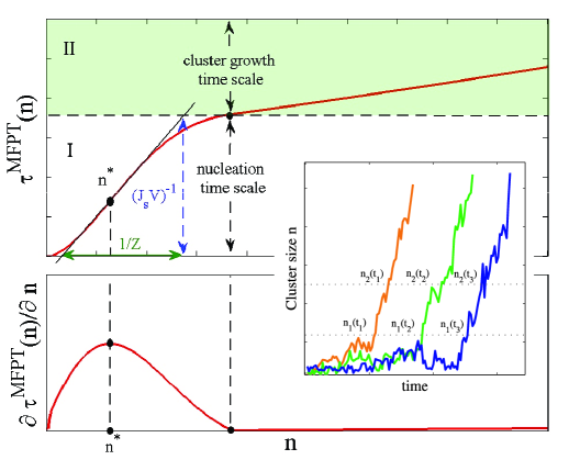
Figure 1: (Color online) Top: Schematic plot of the MFPT distribution for the cluster size $n$ as obtained from simulation (or experimental) data. The regions I and II are associated with nucleation and cluster-growth regimes, respectively. The routine for finding the nucleation characteristics from the MFPT-curve is presented. The gentle slope of the MFPT-curve at the transition value, $n=n^{*}$, is evidence of the smooth form of the nucleation barrier $\Delta G_{n}$ in the vicinity of $n^{*}$, while the location of the inflection point (full circle) below the half-height $1/(2J_{s}V)$ indicates qualitatively on the barrier asymmetry. The pronounced increase of MFPT-curve in the region II appears due to the fact that nucleation and cluster-growth time scales are comparable, and this part of the curve as an inverted one, $n(\tau^{MFPT})$, can be used to estimate the parameters of cluster growth kinetics. Bottom: First derivative of the MFPT distribution, $\partial\tau_{n}^{MFPT}/\partial n$. Here, the maximum is associated with the inflection point, which is directly located at the critical value of cluster size, $n=n^{*}$. Position of the next extremum (minimum) on $(\partial\tau_{n}^{MFPT}/\partial n)_{n>n^{*}}$ corresponds to the nucleation time scale $\tau_{n}=1/(2J_{s}V)$ as defined from the main MFPT distribution $\tau_{n}^{MFPT}$. Inset: Typical cluster growth curves obtained from the independent simulations.

Nucleation-growth kinetics is characterized by the nucleation time scale $\tau_{n}=1/(J_{s}V)$ and the cluster-growth time scale $\tau_{gr}$. The ratio between these time scales distinguishes the separate cases for the numerical treatment within the MFPT method: (i) If $\tau_{n}\gg\tau_{gr}$, then $\tau_{n}^{MFPT}$ demonstrates a clear defined plateau of the height $\tau_{n}=1/(J_{s}V)$, that simplifies significantly accurate estimation of the nucleation rate; (ii) If these time scales are comparable, $\tau_{n}\sim\tau_{gr}$, then the errors can appear in the estimation of $\tau_{n}$, since the boundary between nucleation and growth in MFPT distribution is smeared.

Furthermore, the MFPT method gives a convenient tool to extract the characteristics of nucleus growth kinetics, which follows the nucleation regime in the MFPT distribution (see Fig. 1). In fact, the inverted MFPT distribution, $n(\tau^{MFPT})$, has the statistical meaning of the most probable cluster growth law for the growth regime of the MFPT curve.

Following Ref. ²⁷, the growth law of a cluster can be taken in general form as

$$R(t)=R_{*}+(\mathcal{G}_{cl}t)^{\nu},$$ (9)

where $R$ and $R_{*}$ is the radius of the growing cluster and the critically-sized cluster, respectively; $\nu$ is the growth exponent and $\mathcal{G}_{cl}$ is the growth constant, which has a dimension of $[m^{1/\nu}/s]$. Then, the growth rate is $G(t)=\nu\mathcal{G}_{cl}^{\nu}t^{\nu-1}$, while the acceleration of a cluster growth can be formally defined as $a(t)=\nu(\nu-1)\mathcal{G}_{cl}^{\nu}t^{\nu-2}$. The steady cluster growth with a constant growth rate corresponds to the particular case of $\nu=1$, where the growth rate coincides with the growth factor, i.e. $G(t)=\mathcal{G}_{cl}=\mathrm{const}$, otherwise (at $\nu\neq 1$) one has the process with unsteady growth rate ²⁸. Further, taking into account that the volume of a growing cluster evolves with time as $V(t)=c_{g}[R(t)]^{3}$ and $N(t)=\rho_{cl}V(t)$, where $c_{g}$ is a dimensionless cluster-shape factor ($c_{g}=4\pi/3$ in a case of the sphere) and $\rho_{cl}$ is the density of the cluster-phase, one can write the growth law in the extended form:

$$n(t,t_{c})=n^{*}\left[1+\mathcal{G}_{cl}^{3\nu}(t-t_{c})^{3\nu}\frac{\rho_{cl}c_{g}}{n^{*}}+3\mathcal{G}_{cl}^{2\nu}(t-t_{c})^{2\nu}\left(\frac{\rho_{cl}c_{g}}{n^{*}}\right)^{\frac{2}{3}}+3\mathcal{G}_{cl}^{\nu}(t-t_{c})^{\nu}\left(\frac{\rho_{cl}c_{g}}{n^{*}}\right)^{\frac{1}{3}}\right].$$ (10)

Here, the lag-time $t_{c}$ defines the appearance of the critically-sized cluster. Then, the term $n(\tau^{MFPT})$ can be fitted for the growth regime by Eq. (10) to extract the growth characteristics: the cluster-shape factor $c_{g}$, the growth constant $\mathcal{G}_{cl}$ and the growth exponent $\nu$. At rapid growth of small clusters the last two contributions in Eq. (10) can be neglected, and the growth law takes the form ²⁸

$$n(t,t_{c})\simeq n^{*}+c_{g}\rho_{cl}\mathcal{G}_{cl}^{3\nu}(t-t_{c})^{3\nu},$$ (11)

where $\nu$ is positive.

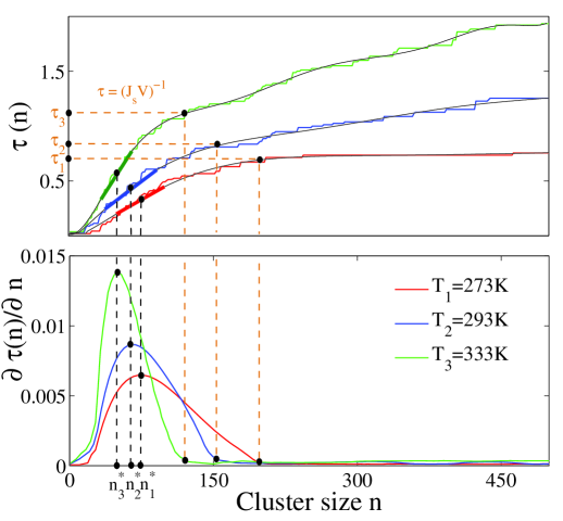
Figure 2: (Color online) Top: Direct MFPT distributions (stepwise-curves) and their interpolations (smooth solid curves) for the temperatures $T=273$, $293$ and $333$ K. Dots on the curves indicate the inflection points, which define the critical sizes $n^{*}$, and the time scales $\tau=(J_{s}V)^{-1}$ corresponding to the nucleation rates. Thick short lines are the linear parts of the interpolated curves near $n^{*}$ and define the ranges of errors in critical sizes. Note that the errors in the nucleation rates can be also defined as a result of changes in $\tau=(J_{s}V)^{-1}$ due to the correction of different interpolations with the same accuracy in the reproduction of the direct MFPT-distributions. Bottom: First derivative of the MFPT distributions, $\partial\tau_{n}^{MFPT}/\partial n$, for the same temperatures.

3 Computational details

Molecular dynamics simulations were performed in the spirit of previous studies of the structural transformations in this system described in Refs. ^{15, 14} with only difference in the details related with the considered thermodynamic range. We have examined the system composed $N=8\;000$ particles (molecules) interacting via the mW-potential in the cubic cell with the periodic boundary conditions in all directions. The time-step for numerical integration was $1$ fs; and the $NpT$ (number, pressure, temperature) ensemble was applied with $p=1$ atm. Pressure and temperature were controlled via the Nosé-Hoover barostat and thermostat, respectively, acting uniformly throughout the system. The damping thermostat and barostat constants were taken to be $\tau_{T}=\tau_{P}=10$ fs. The parameters of the mW-potential are completely identical to those reported in Refs. ^{15, 14}.

Initially, the set of a hundred of independent samples was prepared and equilibrated at the temperature $T=900$ K on the time scale $50$ ps (i.e. $50\;000$ time-steps). The correspondence of the systems to the vapor phase was directly confirmed by the particle diffusivity and the distinctive particle radial distribution functions. Moreover, following Ref. ¹⁵, the samples were cooled at $10$ K/ns to the desired temperatures from the range $273\leq T/K\leq 373$ (at $p\simeq 1$ atm.). Then, over a time scale $\sim 1\div 10$ ps each a system was ‘equilibrated’ till the disappearance of the pronounced fluctuations in temperature and pressure, after that the initial configurations were stored for the further study of the vapor-to-liquid nucleation process. Note that this cooling procedure is similar to the reported one in Ref. ¹⁰. The following $NpT$-simulations starting from these configurations – a hundred for each considered temperature – were performed to collect the statistics of the independent nucleated events, where the time-dependent cluster size distributions $N_{n}(t)$ were evaluated (for an every run). The averaged time scale for the simulations in this nucleation-growth regime was $50$ ns. On the basis of the found $N_{n}(t)$-distributions, the MFPT-curves were extracted and the nucleation characteristics were estimated according to the scheme presented above. After this, the critical sizes $n^{*}$ defined from the MFPT-curves were used at the retreatment of the simulation data with the aim to define the distributions of the energy $\omega$ over the reaction coordinate $\lambda$.

An identification of the particles, which belong to liquid phase, was performed in the spirit of the Stillinger rule ²⁹. First, the particles are “neighbors” (or bonded) if the distance between their centers is less than $r_{s}$, where $r_{s}$ is the position of the first minimum in the pair correlation function of the liquid phase (at the same conditions). Further, a particle is considered as a liquid-like if it has, at least, four neighbors .

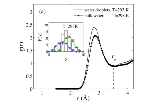
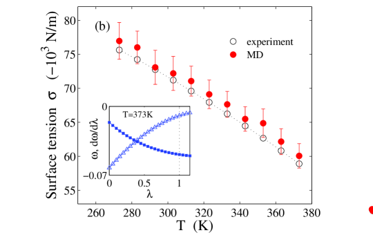
Figure 3: (Color online) (a) Radial distribution function $g(r)$ of liquid water as resulted from the mW-model: results for bulk water at $T=298$ K and $p=0$ (full circles) reported in Ref. ¹⁴, data for the bulk range of critically-sized droplets at $T=293$ K and $p=1$ atm. Inset: Distribution of the first coordination number for the water molecules of a critically-sized liquid droplet at the temperature $T=293$ K. The histogram corresponds to the total distribution; the line with triangles present an impact from the bulk molecules, $z$; and the line with rotated triangles shows the contribution of the surface molecules, $z^{\prime}$. The data are averaged over set of runs. (b) Main: Temperature dependence of the surface tension $\sigma$. The simulation results show the averages (full circles) and standard deviations (error bars) from independent runs; experimental data are presented by open circles, whereas the dotted line is the interpolation by $\sigma(T)=B[(T_{c}-T)/T_{c}]^{m}\{1+b[(T_{c}-T)/T_{c}]\}$, $B=235.6$ N/m, $b=-0.625$, $m=1.256$ and $T_{c}=647.15$ K ³². Inset: Surface energy and slope of the surface energy $\partial\omega/\partial\lambda$ as functions of $\lambda=(N/N_{c})^{1/3}$ for a growing water droplet. At the critical size $N=N_{c}$ one has $\lambda=1$. The presented results are outcome of a single simulation run.

4 Results

In Fig. 2 the obtained MFPT distributions $\tau_{n}^{MFPT}$ and their derivatives $\partial\tau_{n}^{MFPT}/\partial n$ at the temperatures $T=273$, $293$ and $333$ K are presented as an example. On the basis of the defined values of the critical size $n^{*}$ and nucleation rate $J_{s}=(\tau^{MFPT}V)^{-1}$, the values of the Zeldovich factor were extracted within Eq. (8). The typical $\lambda$-dependences of the surface energy and its derivative as obtained from a single run are shown in the inset of Fig. 3(b). The averages of the slope $\langle d\omega/d\lambda\rangle_{\lambda}$ over different runs were used to estimate Eq. (2) by means of the trapezoidal method. The smooth character of the curves allows one to restrict oneself by the method and to exclude higher order integration schemes ³⁰. It is necessary to note that errors in the critical size $n^{*}$ have not been considered at the estimation of the surface tension with Eq. (2).

Coordination number. – The inset of Fig. 3(a) shows the distribution of the first coordination number for the water molecules generated a droplet of the critical size in the system at the temperature $T=293$ K. The presented histogram is the cumulative result of the distributions for surface and bulk molecules. Remarkably, these distributions (for bulk and surface molecules) are symmetric ones as well as reproducible by the Gaussian functions. Further, the averaged values of the coordination numbers $z$ and $z^{\prime}$ are extracted from the distributions and appear to be $5.8$ and $3.93$, respectively, for the case. Other important observation is that the term $z$ is practically unchangeable with temperature, whereas the coordination number in a surface layer demonstrates a smooth insignificant decrease with the temperature increasing [for comparison, from $z^{\prime}(T=293\;\mathrm{K})=3.93$ to $z^{\prime}(T=353\;\mathrm{K})=3.47$].

Moreover, the value of the coordination number for bulk molecules in the droplets coincides with the found value of $z$ extracted on the basis of the integral definition ³¹

$$z=4\pi\rho_{l}\int_{0}^{r_{c}}r^{2}g(r)dr,$$ (12)

where $r_{c}$ is the first minimum position in the radial distribution function $g(r)$. Nevertheless, the found value $z(T=293\;\mathrm{K})=5.8$ differ from the result of Molinero and Moore ¹⁴ obtained within the mW-model for the bulk water, $z(T=298\;\mathrm{K})=5.1$. To understand the reasons of the discrepancy, we compare the corresponding radial distribution functions in Fig. 3(a). As can be seen, the intensity of the first maximum of $g(r)$ is higher for the case of the water droplets, although the maximum is located at a lower distance. This feature indicates that the liquid phase is characterized by the more pronounced short-range ordering for the case of the microscopically small nucleated clusters than for the equilibrium liquid phase considered in Ref. ¹⁴.

Surface tension. – In Fig. 3(b), the temperature dependence of the surface tension of the critically-sized nuclei is presented. The results obtained from simulation data demonstrate the known decrease of the surface tension with temperature  and reproduce precisely the experimental data of this term for a planar liquid-vapor interface ³². Such a good agreement of our results with experimental data is unexpected because of the two next reasons, mainly. First, in contrast to an inherent water system, the mW-model excludes the long-range intermolecular interactions, which still can have an influence on the interface effects. Second, no adjustment of simulation data was performed to take into account the finite size effects. Thereby, the corrections to surface free energy in the spirit of the Tolman’s ansatz, which are appeared to be proportional to the inverse linear size of the critical nucleus, were unconsidered for the surface tension.

On the other hand, the surface tension of a planar interface was recently defined with the mW-model for the temperatures $250\leq T/K\leq 350$ ³³. The values of the surface tension reported in Ref. ³³ have the lower values in comparison with the values presented in Fig. 3(b) for the water droplets, and the difference is about $5\div 10$ percents for the same temperature range. Although this difference could be attributed to the Tolman length with the negative value, like it was reported by Kiselev and Ely ³⁴ for the liquid-ice surface tension, we assume that our values of $\sigma$ can be overestimated because of the neglect the three-particle interactions by computational protocol within Eq. (1).

Nevertheless, the surface tension decrease with the temperature is directly consistent with the temperature decreasing of $u(\widehat{r}_{ij})$, of the surface coordination number [or the increase of the difference $(z-z^{\prime})$] and of the surface particle density, where the last two contributions are practically counterbalanced by each other .

Recalling the previous debates ³⁵, the temperature range investigated here can contain the inflection points in the vapor-liquid surface tension of water. The results, presented in Fig. 3(b), indicate on the absence of the clear detected inflections in the $T$-dependence of the surface tension.

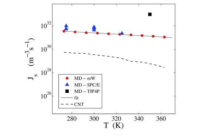
Figure 4: (Color online) Temperature dependence of the homogeneous droplet (vapor-to-liquid) nucleation rate $J_{s}(p\simeq 1\;\mathrm{atm},T)$ in water. Comparison of the simulation results with the mW-model [the vapor density is $\rho_{v}\in[1.12;\;1.55]\times 10^{-2}$nm^-3], with the atomistic SPC/E-model from Ref. ¹⁰ [the density is $\rho_{v}\in[1.23;\;1.86]\times 10^{-2}$nm^-3], with the atomistic TIP$4$P-model from Ref. ¹¹ [the numerical density is $\rho_{v}=1.55\times 10^{-2}$nm^-3] and the treatment of nucleation data within the CNT. Solid line show the best fit by means of the function $J_{s}(p\simeq 1\;\mathrm{atm},T)\propto\exp(-0.00092\;T^{1.4})$.

Steady-state nucleation rate. – In Fig. 4, the steady-state nucleation rates obtained from the MFPT treatment of the simulation data with the mW-model are presented as a function of temperature (see also Table 1). The presented data cover the density range $\rho_{v}$ from $1.14\times 10^{-2}$nm^-3 to $1.55\times 10^{-2}$nm^-3. As can be seen, the values of $J_{s}(T)$ compare well with those obtained for the same density range by Matsubara et al. with the atomistic SPC/E-model ¹⁰. Nevertheless, as contrasted to results of Ref. ¹⁰, which are scattered over ($J_{s},T$)-plot, the values of the nucleation rate $J_{s}$ obtained within the mW-model demonstrate the smooth decrease with temperature over the considered temperature range. Moreover, this decrease is well-reproduced by the dependence $\ln[J_{s}(T)]=-0.00092\;T^{1.4}+75$. Among all the data presented on Fig. 4(a), the highest value of the nucleation rate appears from the simulations of Ref. ¹¹ with the TIP$4$P-model.

On the other hand, it is attractive to test the dependence $J_{s}(T)$ within the CNT treatment with the extracted values of the other nucleation characteristics. So, the original Becker-Döring formulation yields

$$J_{s}^{CNT}=\frac{\rho_{v}^{2}}{\rho_{l}}\sqrt{\frac{2\sigma_{\infty}}{\pi m}}\exp\left(-\frac{\Delta G_{n^{*}}}{k_{B}T}\right),$$ (13)

where the barrier can be taken as

$$\frac{\Delta G_{n^{*}}}{k_{B}T}=3\pi(n^{*}Z)^{2},$$ (14)

and $\sigma_{\infty}$ is the surface tension for a planar liquid-vapor interface ³². As can be seen from Fig. 4, although the both dependencies demonstrate a similar behavior decaying with temperature, the pure simulation results for nucleation rate have in two orders higher values in comparison with $J_{s}^{CNT}$. This is evidence of the difficulties at the description of the droplet nucleation in water by means of the CNT, which are similar with those reported earlier for the studies with the atomistic models ^{13, 10} as well as with the experimental data (see Fig.3 of Ref.³⁶).

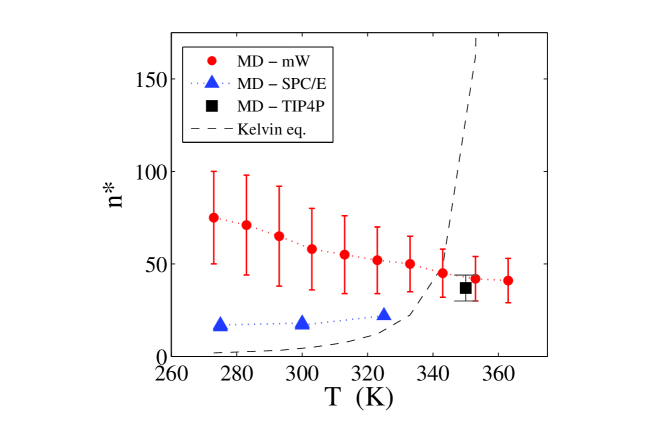
Figure 5: (Color online) Temperature dependence of the critical cluster size, determined from simulations within the different models of potential fields (mW-model, SPC/E ¹⁰, TIP$4$P ¹¹), compared to prediction by Kelvin equation. In the case of the mW-model, error bars are defined by a width of the curvature range in MFPT-distributions.

Critical cluster (droplet) size. – Figure 5 illustrates the temperature dependence of the critical cluster size $n^{*}$, where the simulation results with the mW-model are compared with the simulation data of Matsubara et al. ¹⁰ and of Yasuoka et al. ¹¹ as well as with the predictions of the Kelvin equation

$$n^{*}=\frac{32\pi}{3}\frac{\sigma_{\infty}^{3}}{\rho_{l}^{2}[k_{B}T\ln(p/p^{s})]^{3}}.$$ (15)

Here $p^{s}$ is the saturated water vapor pressure ³⁷.

First, for the mW-model the critical cluster size reveals a slight decrease with temperature from $n^{*}=75$ to $40$ particles over the temperature range $273\leq T/K\leq 363$. This change of the cluster size means the decrease of the droplet radius from $4$ to $3.3$ of the averaged water molecule diameters. Obviously, the change is insignificant. Moreover, the observed decrease is masked by errors, which were defined as the curvature range width in the MFPT-distributions (see Fig. 2). The range of errors is $\pm(10\div 25)$ particles, that is awaited to be reasonable, since it covers only a few surface part of a water droplet (Fig. 6). In addition, according to the definition within the MFPT-method these errors should be considered as the probable deviations from $n^{*}$ in a statistical sense. The comparison with the results obtained for the atomistic models (TIP$4$P and SPC/E) reveals that the values of $n^{*}$ obtained within the mW-model overestimate the data of the SPC/E-model, but are in agreement with a single value found by Yasuoka et al. in simulations with the TIP$4$P-model.

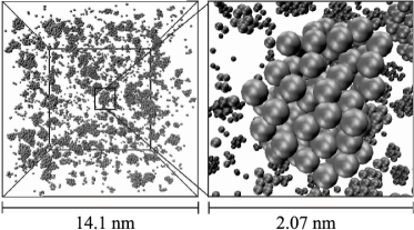
Figure 6: (Color online) Left: Snapshot of the water system at the temperature $T=293$ K and the pressure $p=1$ atm. at the moment, when the critically-sized droplets are appearing. Right: Growing droplet of the same system.

Further, the mW-model result for $n^{*}(T)$-curve is different from the predictions of Eq. (15), which yields the increase of $n^{*}$ with the temperature $T$ (see Fig. 5) . However, it should be noted that as far as the predictions of the Kelvin equation are concerned, it gives the values $n\simeq 2\div 12$ molecules for the temperature range $273\leq T/K\leq 363$ and the pressure $p=1$ atm. In terms of the linear cluster sizes, these values correspond to $1\div 2$ water molecule diameters. It is clear that the treatment of the stability of such a small cluster from the thermodynamic point of view, which requires the availability of the separated surface and bulk regions of the cluster, is impossible. 

Nucleation barrier and the Zeldovich factor. – The temperature dependence of the next nucleation characteristic, the Zeldovich factor $Z$, is presented in Fig. 7. As can be seen, this quantity decreases from the value $0.028$ to $0.014$ with the decrease of the temperature $T$ (see also Table 1). Such a behavior is a direct evidence that the nucleation barrier loses its sharpness and becomes more smoother with the decreasing the temperature. This is qualitatively in an agreement with the prediction of the CNT ²⁷. Moreover, if one assumes that the CNT yields the correct results for the vapor-to-liquid nucleation of water then it is possible to define the nucleation barrier by means of the simple relation (14). The direct evaluation yields the correct tendency of the temperature dependence for the nucleation barrier, though this tendency is not so pronounced one as it could be expected for a sufficiently wide temperature range considered here. According to the CNT, the nucleation driving force $|\Delta\mu|$, growing with the decrease of $T$, must reduce the nucleation barrier ²⁷.

Within Eq. (14) and simulation results one has that the nucleation barrier decreases from $\beta\Delta G_{n^{*}}^{MD}=12\pm 2.7$ to $\beta\Delta G_{n^{*}}^{MD}=9.7\pm 2.5$ with the decrease of the temperature from $T=363$ to $273$ K. On the other hand, the temperature dependence of the nucleation barrier as predicted by the CNT is defined by

$$\Delta G_{n^{*}}\propto\frac{\sigma_{\infty}^{3}}{\rho_{l}^{2}|\Delta\mu|^{2}},$$

where $|\Delta\mu|$ is the chemical potential difference of particles in the vapor and in the liquid phase. So, the observed behavior of the nucleation barrier can be explained for the case, where the change of $\sigma_{\infty}^{3}/\rho_{l}^{2}$ with the temperature is completely counterbalanced by the change of $|\Delta\mu|^{3}$.

Remarkably, the comparable values for the nucleation barrier arise with the atomistic SPC/E model (see Table I in Ref. ¹⁰), where the barrier changes from $\beta\Delta G_{n^{*}}=8.1$ to $\beta\Delta G_{n^{*}}=6.7$ with the temperature decreasing from $T=325$ to $275$ K. Thus, the observed results for the nucleation barrier can not be considered as a consequence of the coarse-grained character of particle interactions in the mW-model.

Table 1: Simulation results: system temperature $T$ (K); vapor number density $\rho_{v}$ ($\times 10^{-2}$ nm^-3); critical cluster size $n^{*}$; nucleation barrier $\Delta G/k_{B}T$; nucleation rate $J_{s}$ ($\times 10^{32}$ m^-3s${}^{-1})$; the Zeldovich factor $Z$.

$T$	$\rho_{v}$	$n_{c}$	$\Delta G/k_{B}T$	$J_{s}$	$Z$
273	$1.548\pm 0.095$	$75\pm 25$	$9.72\pm 2.55$	$0.35$	$0.0135\pm 0.0009$
283	$1.462\pm 0.060$	$71\pm 27$	$9.76\pm 2.06$	$0.30$	$0.0143\pm 0.0008$
293	$1.426\pm 0.077$	$65\pm 27$	$9.78\pm 2.39$	$0.26$	$0.0157\pm 0.0008$
303	$1.425\pm 0.051$	$58\pm 22$	$10.07\pm 1.57$	$0.24$	$0.0182\pm 0.0007$
313	$1.353\pm 0.062$	$55\pm 21$	$10.21\pm 2.25$	$0.21$	$0.0189\pm 0.0009$
323	$1.313\pm 0.047$	$52\pm 18$	$10.43\pm 2.18$	$0.19$	$0.0202\pm 0.0008$
333	$1.250\pm 0.037$	$50\pm 15$	$10.98\pm 2.53$	$0.17$	$0.0216\pm 0.001$
343	$1.224\pm 0.032$	$45\pm 13$	$11.10\pm 1.70$	$0.15$	$0.0241\pm 0.0007$
353	$1.174\pm 0.045$	$42\pm 12$	$11.50\pm 1.94$	$0.13$	$0.0262\pm 0.0009$
363	$1.140\pm 0.033$	$41\pm 12$	$11.97\pm 2.17$	$0.11$	$0.0275\pm 0.001$

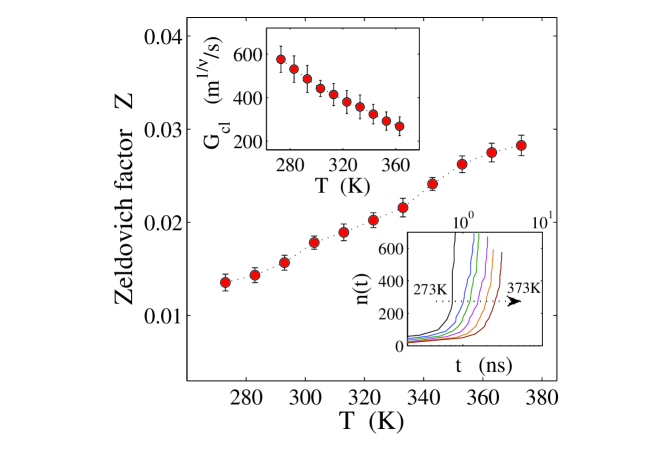
Figure 7: (Color online) Main: Temperature dependence of the Zeldovich factor $Z$ as defined by the MFPT method on the basis of the simulations with the mW-model. Top inset: Temperature dependence of the growth factor $\mathcal{G}_{cl}$, which is found from the fit of Eq. (11) to the simulation data. The growth exponent $\nu=1.3$ and the term $A=c_{g}\rho_{l}(\mathcal{G}_{cl}t_{c})^{3\nu}/n^{*}=1.16\pm 0.2$ appear to be invariant respective the temperature. Error bars show the standard deviations from the averages. Bottom inset: Growth curves of the liquid water droplets emerging in the vapor phase at the temperatures $273\leq T/K\leq 373$.

Growth laws of the nucleated droplets. – Bottom inset of Fig. 7 shows the growth curves of the liquid droplet at the different temperatures, which were found from the statistical treatment of simulation data by means of the MFPT approach as it was discussed above. Hence, these curves depict the most probable growth laws in a statistical sense. As can be seen from the figure, at the lower temperature the droplet growth occurs faster. At the same time, all the curves are well reproduced by Eq. (11), and the fitting to the simulation data yields the following features. The growth exponent $\nu$ in Eq. (11) appears to be invariant over the temperature $T$ and it takes the value $\nu=1.3$ at all the considered temperatures. This indicates that the increasing the linear size, i.e. the radius, averaged over all the directions of the liquid droplet follows for all the temperatures the growth law $R(t)=(\mathcal{G}_{cl}t)^{1.3}$, herewith, the droplet growth itself is unsteady.

Further, the growth factor $\mathcal{G}_{cl}$ decreases with the increase of the temperature $T$ (see top inset of Fig. 7), that characterizes the faster droplet growth at the lower temperatures. Following Ref. ²⁸, Eq. (11) can be written in the rescaled form:

$$n(\xi)/n^{*}\simeq 1+A(\xi-1)^{3\nu},$$ (16)

where $A=c_{g}\rho_{l}(\mathcal{G}_{cl}t_{c})^{3\nu}/n^{*}$ and $\xi=t/t_{c}$ is the rescaled time. We found that in accordance with the rescaled form (16) all the growth curves collapse onto a single curve independently of the temperature. In addition, the parameter $A$ in Eq. (16) takes the same value for all the considered temperatures, i.e. $A=1.16\pm 0.2$. This can be evidence of the generic features of the water droplet growth process. Remarkably, this result is correlated with the features of the crystal growth kinetics for a model glassy system under shear drive, which were reported in Ref. ²⁸.

Shape and sphericity of the nucleated droplets. – Other issue, which is crucial in the CNT, is related with the shape and the anisotropy of the growing droplets ^{16, 38}. A convenient way to perform this study in our case is to use the asphericity parameter in the next definition:

$$S_{0}=\left\langle\frac{(I_{xx}-I_{yy})^{2}+(I_{xx}-I_{zz})^{2}+(I_{yy}-I_{zz})^{2}}{2(I_{xx}+I_{yy}+I_{zz})^{2}}\right\rangle,$$

where

$$I_{\alpha\beta}=\sum_{i=1}^{n^{*}}m_{0}(r_{i}^{2}\delta_{\alpha\beta}-r_{i\alpha}r_{i\beta})$$

is the components of the moment of inertia tensor associated with a droplet, $m_{0}$ is the molecule mass, $\alpha,\beta\in\{x,y,z\}$ are the components of the vector $\vec{r}$ between the droplet center-of-mass and molecule $i$; the brackets $\langle\ldots\rangle$ mean the statistical average over critically-sized droplets of the different simulation runs. This definition of a asphericity parameter sets the characterization: for a spherical droplet one has $S_{0}=0$, whereas for an elongated and string-like cluster one obtains $S_{0}\to 1$. We found that independently on the particular conditions (temperature, vapor density) the asphericity parameter for the considered ($p,T$)-range is $S_{0}\simeq 0.008\pm 0.0002$. It indicates on the nucleated water droplets of the sphere-like form, which is also confirmed by a visual inspection of snapshots (Fig. 6). We remark here, this result is not the same with the findings of Refs. ^{11, 10}, where the detected critical clusters in water had the significant deviations from a spherical form. A possible reason affecting the observed discrepancy could be different cluster definitions applied by Matsubara et al. in Ref. ¹⁰ and used in the present study within the statistical treatment. In addition, the low values for the nucleated droplets were obtained in Ref. ¹⁰, $n^{*}\simeq 16\div 22$ partilces, and the pronounced deviation from a spherical form can be considered as a signature of the finite size effects: a weak structural rearrangement in such a system raises the significant change of its shape.

5 Conclusions

The coarse-grained models for particle interactions in molecular systems provide the good opportunity to study early stages of the phase transitions by means of the numerical simulations. In this work, the processes of the steady-state homogeneous vapor-to-liquid nucleation and the growth of liquid droplets in water were considered within the mW-model, which treats the molecular interactions excluding any details of the direct oxygen-hydrogen interactions and electrostatics. Despite the apparent coarsening in the description of the molecular interactions, we have shown that the mW-model provides interesting information concerning the droplet nucleation in water vapor, thereby complementing the simulation results obtained earlier within all-atom models of water such as TIP$4$P and SPC/E ^{39, 31, 11, 10}. It is necessary to note, the results reported here are obtained on the basis of the extended statistical treatment within the MFPT approach and the thermodynamic integration scheme.

The surface tension of the nucleated droplets was computed within an approximation that is restricted by the consideration of the two-particle interactions only without handling the three-particle contribution to the energy of system. The obtained values demonstrate the decrease of the surface tension with the temperature growth. It is necessary to note that the applied numerical scheme gives the higher values for the liquid-vapor surface tension of the droplets in comparison with the values for the liquid-vacuum surface tension of a planar interface reported in Ref. ^{33, 14}. We suppose that this difference is rather a result of the approximations applied to the surface tension definition than the mW-model product.

Further, the evaluated values of the steady-state nucleation rate are comparable with the results for all-atom models as well as with the treatments within the classical nucleation theory. Unfortunately, we could not to perform the direct comparison of the obtained nucleation rates with the experimental data, because we found no experimental $J_{s}$ for the ($p,T$)-line considered here. Nevertheless, quantitative extrapolation of the obtained outcomes indicates on the difference between simulated and experimental results, that is similar with the known difference between the experimental data and the CNT predictions ^{40, 9}. On the other hand, for the critical size of the nucleated droplet we found the values within the range $30\div 100$ particles, which are expected to be comparable with the experimental data (Fig. $13$ in Ref. ⁹). So, the additional studies are highly desirable in this field.

According to our results, the growth of nucleated droplets in the system is characterized by the remarkable features: the growth law of the droplet radius follows the power law, $R(t)\propto t^{1.3}$, and the growth is not steady (with the time-dependent growth rate $G(t)\propto t^{0.3}$). Moreover, the simple rescaling on the critical droplet characteristics yields the unified form of the growth law at all the considered temperatures.

Finally, we found that the critically-sized droplets have a shape, which is close to spherical one. Note, that the deviations from spherical shape of the water droplets at homogeneous nucleation, which were established for the SPC/E-model by Matsubara et al. (see Ref. ¹⁰), could be simply originated from the extremely low obtained values for the critical size $n^{*}$.

6 Acknowledgments

The authors acknowledge B.N. Hale for helpful correspondence and R.M. Khusnutdinoff for many useful discussions.

References

- 1 Wölk, J.; Strey, R. J. Phys. Chem. B 2001, 105, 11683-11701.
- 2 Kim, Y. J.; Wyslouzil, B. E.; Wilemski, G.; Wölk, J.; Strey, R. J. Phys. Chem. A 2004, 108, 4365-4377.
- 3 Manka, A. A.; Brus, D.; Hyvärinen, A. -P.; Lihavainen, H.; Wölk, J.; Strey, R. J. Chem. Phys. 2010, 132, 244505 1-10.
- 4 Brus, D.; Ždímal, V.; Uchtmann, H. J. Chem. Phys. 2009, 131, 074507 1-9.
- 5 Brus, D.; Ždímal, V.; Smolík, J. J. Chem. Phys. 2008, 129, 174501 1-8.
- 6 Mikheev, V. B.; Irving, P. M.; Laulainen, N. S.; Barlow, S. E.; Pervukhin, V. V. J. Chem. Phys. 2002, 116, 10772-10786.
- 7 Luijten, C. C. M.; Bosschaart, K. J.; van Dongen, M. E. H. J. Chem. Phys. 1997, 106, 8116-8123.
- 8 Heist, R. H.; He, H. J. Phys. Chem. Ref. Data 1994, 23, 781-804.
- 9 Viisanen. Y.; Strey, R.; Reiss, H. J. Chem. Phys. 1993, 99, 4680-4692.
- 10 Matsubara, H.; Koishi, T.; Ebisuzaki, T. J. Chem. Phys. 2007, 127, 214507 1-11.
- 11 Yasuoka, K.; Matsumoto, M. J. Chem. Phys. 1998, 109, 8451-8462.
- 12 Merikanto, J.; Vehkamäki, H.; Zapadinsky, E. J. Chem. Phys. 2004, 121, 914 1-24.
- 13 Chen, B.; Siepmann, J. I.; Klein, M. L. J. Phys. Chem. A 2005, 109, 1137-1145.
- 14 Molinero, V.; Moore, E. B. J. Phys. Chem. B 2009, 113, 4008-4016.
- 15 Moore, E. B.; Molinero, V. Nature 2011, 479, 506-508.
- 16 Reinhardt, A.; Doye, J. P. K. J. Chem. Phys. 2012, 136, 054501 1-11.
- 17 Bartell, L. S.; Turner, G. W. J. Phys. Chem. B 2004, 108, 19742-19747.
- 18 Mokshin, A. V.; Yulmetyev, R. M.; Khusnutdinoff, R. M.; Hanggi, P. J. Phys.: Cond. Mat. 2007, 19, 046209 1-16.
- 19 Berry, M. V.; Durrans, R. F.; Evans, R. J. Phys. A: Gen. Phys. 1972, 5, 166-70.
- 20 Horsch, M.; Hasse, H.; Shchekin, A. K.; Agarwal, A.; Eckelsbach, S.; Vrabec, J.; Müller, E. A.; Jackson, G. Phys. Rev. E. 2012, 85, 031605 1-12.
- 21 Wedekind, J.; Strey, R.; Reguera, D. J. Chem. Phys. 2007, 126, 134103 1-7.
- 22 Mokshin, A. V.; Barrat, J.-L. Phys. Rev. E 2008, 77, 021505 1-7.
- 23 Mokshin, A. V.; Barrat, J.-L. J. Chem. Phys. 2009, 130, 034502 1-6.
- 24 Frenkel, J. Kinetic Theory of Liquids; Oxford University Press: London, 1946.
- 25 Hansen, J. P.; McDonald, I. R. Theory of Simple Liquids; Academic Press: New York, 2006.
- 26 Hänggi, P.; Talkner, P.; Borkovec, M. Rev. Mod. Phys. 1990, 62, 251-342.
- 27 Kashchiev, D. Nucleation: Basic Theory with Applications; Butterworth Heinemann: Oxford, U.K., 2000.
- 28 Mokshin, A. V.; Barrat, J.-L. Phys. Rev. E 2010, 82, 021505 1-9.
- 29 Stillinger, F. H. J. Chem. Phys. 1963, 38, 1486-1494.
- 30 Ytreberg, F. M.; Swendsen, R. H.; Zuckerman, D. M. J. Chem. Phys. 2006, 125, 184114 1-11.
- 31 Khusnutdinoff, R. M.; Mokshin, A. V. Physica A 2012, 391, 2842-2847.
- 32 IAPWS Release on Surface Tension of Ordinary Water Substance, IAPWS, 1994 (http:// www.iapws.org/relguide/surf.pdf).
- 33 Baron, R.; Molinero, V. J. Chem. Theory Comput 2012, in press, (DOI: 10.1021/ct300121r).
- 34 Kiselev, S. B.; Ely, J. F. Physica A 2001, 299, 357-370.
- 35 Lü, Y. J.; Wei, B. Appl. Phys. Lett. 2006, 89, 164106 1-3 and references therein.
- 36 Hale, B. N. J. Chem. Phys. 2005, 122, 204509 1-3.
- 37 Alexandrov A. A.; Grigoriev B. A. Tables of Thermophysical Properties of Water and Steam MEI, Moscow, Russia, 1999.
- 38 Rodney, D.; Tanguy, A.; Vandembroucq, D. Modelling Simul. Mater. Sci. Eng. 2011, 19, 083001 1-49.
- 39 Khusnutdinoff, R. M.; Mokshin, A. V. J. Non-Cryst. Solids 2011, 357, 1677-1684.
- 40 Hale, B. N.; Thomason, M. Phys. Rev. Lett. 2010, 105, 046101 1-4.