Forbidden oxygen lines in comets at various heliocentric distances

We present a study of the three forbidden oxygen lines [OI] located in the optical region (i.e., $5577.339\leavevmode\nobreak\ \r{A}$ (the green line), $6300.304\leavevmode\nobreak\ \r{A}$ and $6363.776\leavevmode\nobreak\ \r{A}$ (the two red lines)) in order to better understand the production of these atoms in cometary atmospheres. The analysis is based on 48 high-resolution and high signal-to-noise spectra collected with UVES at the ESO VLT between 2003 and 2011 referring to 12 comets of different origins observed at various heliocentric distances. The flux ratio of the green line to the sum of the two red lines is evaluated to determine the parent species of the oxygen atoms by comparison with theoretical models. This analysis confirms that, at about 1 AU, H₂O is the main parent molecule producing oxygen atoms. At heliocentric distances ¿ 2.5 AU, this ratio is changing rapidly, an indication that other molecules are starting to contribute. CO and CO₂, the most abundant species after H₂O in the coma, are good candidates and the ratio is used to estimate their abundances. We found that the CO₂ abundance relative to H₂O in comet C/2001 Q4 (NEAT) observed at 4 AU can be as high as $\sim$70$\%$. The intrinsic widths of the oxygen lines were also measured. The green line is on average about 1 km s^-1 broader than the red lines while the theory predicts the red lines to be broader. This might be due to the nature of the excitation source and/or a contribution of CO₂ as parent molecule of the $5577.339\leavevmode\nobreak\ \r{A}$ line. At 4 AU, we found that the width of the green and red lines in comet C/2001 Q4 are the same which could be explained if CO₂ becomes the main contributor for the three [OI] lines at high heliocentric distances.

1 Introduction

Comets are small bodies formed at the birth of the Solar system 4.6 billion years ago. Since they did not evolve much, they are potential witnesses of the physical and chemical processes at play at the beginning of our Solar system (Ehrenfreund & Charnley, 2000). Their status of ”fossils” gives them a unique role to understand the origins of the Solar system, not only from the physical and dynamical point of view but also from the chemical point of view (thanks to the knowledge of the compounds of the nucleus). When the comet gets closer to the Sun, the ices of the nucleus sublimate to form the coma (the comet atmosphere) where oxygen atoms are detected. Oxygen is an important element in the chemistry of the Solar system given its abundance and its presence in many molecules including H₂O which constitutes 80$\%$ of the cometary ices. Oxygen atoms are produced by the photo-dissociation of molecules coming from the sublimation of the cometary ices. Chemical reactions Eq.(1) to (6) involve possible parent molecules (Bhardwaj & Raghuram, 2012; Festou & Feldman, 1981).

$$\mathrm{H_{2}O+h\nu} \rightarrow \mathrm{H_{2}+O^{*}(^{1}D)}$$ (1)

$$\mathrm{H_{2}O+h\nu} \rightarrow \mathrm{H_{2}+O^{*}(^{1}S)}$$ (2)

$$\mathrm{CO_{2}+h\nu} \rightarrow \mathrm{CO+O^{*}(^{1}D)}$$ (3)

$$\mathrm{CO_{2}+h\nu} \rightarrow \mathrm{CO+O^{*}(^{1}S)}$$ (4)

$$\mathrm{CO+h\nu} \rightarrow \mathrm{C+O^{*}(^{1}D)}$$ (5)

$$\mathrm{CO+h\nu} \rightarrow \mathrm{C+O^{*}(^{1}S)}$$ (6)

Oxygen atoms have been detected in comets through the three forbidden lines observed in emission at 5577.339 Å (the green line), 6300.304 Å and 6363.776 Å (the red lines) (Swings, 1962). These lines are coming from the deexcitation of the upper state (2p⁴)¹S₀ to the (2p⁴)¹D₂ state for the 5577.339 $\AA$ line and from the (2p⁴)¹D₂ state to the (2p⁴)³P_1,2 states for the doublet red lines (see Fig. 1). The lifetime of the oxygen in the ¹D state is $\sim$ 110  s which is much longer than the lifetime of $\sim$1 s for the O(¹S). The measurement of the green line is more difficult owing to its fainter intensity and the many C₂ lines located around it. One of the first theoretical studies was carried out by Festou & Feldman (1981). They reviewed the production rate of O(¹S) and O(¹D) obtained in the laboratory from H₂O, CO and CO₂ photo-dissociations and measured the corresponding ¹S/¹D ratio. Recently, Bhardwaj & Raghuram (2012) made a new model for oxygen atom emissions and calculated the production rate of O(¹S) and O(¹D) for chemical reactions (1) to (6). The estimated ¹S/¹D ratios are significantly different from Festou & Feldman (1981) and are given in Table 1.

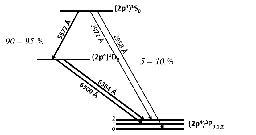
Figure 1: Energy level diagram for [OI] lines.

Parents	Emission rate (s-1)		Ratio
	O(1S)	O(1D)	1S/1D	1S/1Da
H2O	6.4 10-8	8.0 10-7	0.080	$\sim$0.1
CO	4.0 10-8b	5.1 10-8	0.784	$\sim$1
CO2	7.2 10-7	1.2 10-6	0.600	$\sim$1

Table 1: Emission rates and ¹S/¹D ratios relevant to the quiet Sun obtained by Bhardwaj & Raghuram (2012) for photo-dissociation reactions at 1 AU.
^a Ratios obtained by Festou & Feldman (1981) are given in the last column for comparison.
^b This rate comes from Huebner & Carpenter (1979).

Up to now, little systematic researchwork has been done to study these lines at various heliocentric distances because the detection of the forbidden lines requires both high spectral and high spatial resolutions. Morrison et al. (1997) observed oxygen in comet C/1996 B2 (Hyakutake) with the 1-m Ritter Observatory telescope, Cochran & Cochran (2001) and Cochran (2008) analysed [OI] lines in the spectra of 8 comets observed at the McDonald Observatory (see Bhardwaj & Raghuram (2012) for a complete review of these measurements).The present paper reports the results obtained for a homogeneous set of high quality spectra of 12 comets of various origins observed since 2003 with the UVES spectrograph mounted on the 8-m Kueyen telescope of the ESO VLT.
First, we measured the intensities of the three forbidden oxygen lines. Two ratios were evaluated : the ratio between the two red lines, $I_{6300}/I_{6364}$, and the ratio of the green line to the sum of the red lines, $I_{5577}/(I_{6300}+I_{6364})$ which we shall denote as G/R hereafter. The purpose of the latter is to determine the main parent molecule of the oxygen atoms by comparing our results with the Bhardwaj & Raghuram (2012) effective excitation rates. We also followed how the G/R ratio depends on the heliocentric distance by analysing spectra of comets C/2001 Q4 (NEAT) and C/2009 P1 (Garradd) at small and large distances from the Sun.
Finally, we measured the Full Width at Half Maximum (FWHM) of the three lines. There is a long-standing debate on the FWHM measurement because the first observations made by Cochran (2008) are in contradiction with the theory. The intrinsic width of the green line is wider than the red ones while the theory predicts the opposite (Festou, 1981).

In this paper, we present the analysis of the three forbidden oxygen lines in various comets at different heliocentric distances. The observation of all the comets of our sample are explained in section 2. In sections 3 and 4, details about data reduction and data analysis are described. Results of the two ratios and the FWHM of the [OI] lines are given in section 5 followed by discussion in section 6.

2 Observations

Our analysis is based on 12 comets listed in Table 2, considering the two components of 73P/Schwassmann-Wachmann 3 (B and C) as two comets. This sample is characterized by a large diversity. These comets have various dynamical origins (external, new, Jupiter family, Halley type) and are observed at different heliocentric distances (from 0.68 AU to 3.73 AU). Some are split comets like 73P or did a close approach to Earth. Others have been observed at large heliocentric distances like C/2001 Q4 and C/2009 P1. The observing material is made of a selection of 48 high signal-to-noise spectra obtained during the last ten years (Manfroid et al. (2009) ; Jehin et al. (2009) and references therein) with the cross-dispersed echelle spectrograph UVES (Dekker et al., 2000). A dichroic filter splits the light beam into two arms (a red one from 3000 to 5000 $\AA$ and a blue one from 4200 to 11000 $\AA$). In most observations, a slit of 0.45^′′ $\times$ 11^′′ was used. With such a slit, the resolving power is $R=\lambda/\Delta\lambda\leavevmode\nobreak\ =\leavevmode\nobreak\ 110000$ in the red arm where the three [OI] lines are observed. All spectra were recorded with nearly the same instrumental setting. Such a high resolution is needed to isolate the [OI] emission lines from the telluric lines and other cometary lines (C₂, NH₂) (see Fig.2). The slit was always centered on the comet nucleus. For a comet located at 1 AU from the Earth, the spatial area covered by the slit is approximatively 320 km by 8000 km. The size of the slit for each individual spectrum is given in Table 3.

Figure 2: The 6300.304 $\AA$, 6363.776 $\AA$ and 5577.339 $\AA$ oxygen lines (telluric ($\oplus$) and cometary) in a 3600s spectrum of comet 8P/Tuttle obtained in March 2008. Thanks to the high resolution of the UVES spectrograph, the cometary and telluric lines are well separated when the Doppler shift is larger than 15 km s^-1. These spectra are representative of the quality of the sample.

Comet	$Tp$	$e$	a	$q$	$i$	$P$	$T_{J}$	Type (L)
C/2002 V1 (NEAT)	18-02-2003	0.99990	1010	0.10	82	32100	0.06	EXT
C/2002 X5 (Kudo-Fujikawa)	29-01-2003	0.99984	1175	0.19	94	40300	-0.03	EXT
C/2002 Y1 (Juels-Holvorcem)	13-04-2003	0.99715	250.6	0.71	104	3967	-0.23	EXT
C/2001 Q4 (NEAT)	16-05-2004	1.00069	-	0.96	100	-	-	NEW
C/2002 T7 (LINEAR)	23-04-2004	1.00048	-	0.61	161	-	-	NEW
C/2003 K4 (LINEAR)	14-10-2004	1.00030	-	1.02	134	-	-	NEW
9P/Tempel 1	05-07-2005	0.51749	3.1	1.51	11	5.5	2.97	JF
73P-C/Schwassmann-Wachmann 3	07-06-2006	0.69338	3.1	0.94	11	5.4	2.78	JF
73P-B/Schwassmann-Wachmann 3	08-06-2006	0.69350	3.1	0.94	11	5.4	2.78	JF
8P/Tuttle	27-01-2008	0.81980	5.7	1.03	55	13.6	1.60	HF
103P/Hartley 2	28-10-2010	0.69500	3.5	1.06	14	6.5	2.64	JF
C/2009 P1 (Garradd)	23-12-2011	1.00110	-	1.55	106	-	-	NEW

Table 2: Orbital characteristics of the 12 comets and their classification. $T_{p}$ is the epoch of the perihelion (dd-mm-yyyy), $e$ the eccentricity, $a$ is related to the semi-major axis of the orbit (AU), $q$ is the perihelion distance (AU), $i$ represents the inclination on the ecliptic (degrees), $P$ is the period (years), $T_{J}$ is the Tisserand parameter relative to Jupiter. The last data correspond to the classification of the comets according to Levison (1996) : HF and JF mean ”Halley Family” and ”Jupiter family” and gather comets with short period (¡ 200 years) ; EXT and NEW are respectively for external comets ($a$¡$10000$ AU) and new comets ($a$¿$10000$ AU) which came from the Oort Cloud.

Comet	JD - 2 450 000.5	$r$ (AU)	$\dot{r}$ (km s-1)	$\Delta$ (AU)	$\dot{\Delta}$ (km s-1)	Exptime (s)	Slit (${}^{\prime\prime}\times^{\prime\prime}$)	Slit (km $\times$ km)
C/2002 V1 (NEAT)	2 647.037	1.22	-36.51	0.83	7.88	2100	0.45 $\times$ 11.00	271 $\times$ 6 622
C/2002 V1 (NEAT)	2 647.062	1.22	-36.53	0.83	7.99	2100	0.45 $\times$ 11.00	271 $\times$ 6 622
C/2002 V1 (NEAT)	2 649.031	1.18	-37.11	0.84	8.29	2100	0.45 $\times$ 11.00	274 $\times$ 6 702
C/2002 V1 (NEAT)	2 649.056	1.18	-37.11	0.84	8.33	1987	0.45 $\times$ 11.00	274 $\times$ 6 702
C/2002 V1 (NEAT)	2 719.985	1.01	39.76	1.63	42.02	600	0.45 $\times$ 11.00	532 $\times$ 13 004
C/2002 X5 (Kudo-Fujikawa)	2 705.017	1.06	37.01	0.99	29.34	1800	0.45 $\times$ 11.00	323 $\times$ 7 898
C/2002 X5 (Kudo-Fujikawa)	2 705.039	1.07	37.00	0.99	29.40	1800	0.45 $\times$ 11.00	323 $\times$ 7 898
C/2002 X5 (Kudo-Fujikawa)	2 705.060	1.07	36.99	0.99	29.45	1800	0.45 $\times$ 11.00	323 $\times$ 7 898
C/2002 Y1 (Juels-Holvorcem)	2 788.395	1.14	24.09	1.56	-7.24	1800	0.40 $\times$ 11.00	453 $\times$ 12 446
C/2002 Y1 (Juels-Holvorcem)	2 788.416	1.14	24.09	1.56	-7.21	1800	0.40 $\times$ 11.00	453 $\times$ 12 446
C/2002 Y1 (Juels-Holvorcem)	2 789.394	1.16	24.18	1.55	-7.21	1800	0.40 $\times$ 11.00	450 $\times$ 12 366
C/2002 Y1 (Juels-Holvorcem)	2 789.415	1.16	24.19	1.55	-7.18	1800	0.40 $\times$ 11.00	450 $\times$ 12 366
C/2001 Q4 (NEAT)	2 883.293	3.73	-18.80	3.45	-25.42	4500	0.45 $\times$ 11.00	1 126 $\times$ 27 524
C/2001 Q4 (NEAT)	2 883.349	3.73	-18.80	3.45	-25.32	4500	0.45 $\times$ 11.00	1 126 $\times$ 27 524
C/2001 Q4 (NEAT)	2 889.236	3.67	-18.91	3.36	-23.67	7200	0.45 $\times$ 11.00	1 097 $\times$ 26 806
C/2001 Q4 (NEAT)	2 889.320	3.66	-18.91	3.36	-23.54	7200	0.45 $\times$ 11.00	1 097 $\times$ 26 806
C/2002 T7 (LINEAR)	3 131.421	0.68	15.83	0.61	-65.62	1080	0.44 $\times$ 12.00	195 $\times$ 5 309
C/2002 T7 (LINEAR)	3 151.976	0.94	25.58	0.41	54.98	2678	0.30 $\times$ 12.00	89 $\times$ 3 568
C/2002 T7 (LINEAR)	3 152.036	0.94	25.59	0.42	55.20	1800	0.30 $\times$ 12.00	91 $\times$ 3 655
C/2003 K4 (LINEAR)	3 131.342	2.61	-20.34	2.37	-43.12	4946	0.80 $\times$ 11.00	1 375 $\times$ 18 908
C/2003 K4 (LINEAR)	3 132.343	2.59	-20.35	2.35	-42.95	4380	0.60 $\times$ 11.00	1 023 $\times$ 18 748
C/2003 K4 (LINEAR)	3 329.344	1.20	14.81	1.51	-28.23	1500	0.44 $\times$ 12.00	482 $\times$ 13 142
9P/Tempel 1	3 553.955	1.51	-0.21	0.89	8.95	7200	0.44 $\times$ 12.00	284 $\times$ 7 746
9P/Tempel 1	3 554.954	1.51	-0.15	0.89	9.07	7200	0.44 $\times$ 12.00	284 $\times$ 7 746
9P/Tempel 1	3 555.955	1.51	-0.04	0.90	9.19	7200	0.44 $\times$ 12.00	287 $\times$ 7 833
9P/Tempel 1	3 557.007	1.51	0.09	0.90	9.48	9600	0.44 $\times$ 12.00	287 $\times$ 7 833
9P/Tempel 1	3 557.955	1.51	0.20	0.91	9.44	7500	0.44 $\times$ 12.00	290 $\times$ 7 920
9P/Tempel 1	3 558.952	1.51	0.31	0.91	9.55	7500	0.44 $\times$ 12.00	290 $\times$ 7 920
9P/Tempel 1	3 559.954	1.51	0.43	0.92	9.68	7500	0.44 $\times$ 12.00	293 $\times$ 8 007
9P/Tempel 1	3 560.952	1.51	0.55	0.93	9.80	7800	0.44 $\times$ 12.00	297 $\times$ 8 094
9P/Tempel 1	3 561.953	1.51	0.66	0.93	9.91	7200	0.44 $\times$ 12.00	297 $\times$ 8 094
9P/Tempel 1	3 562.956	1.51	0.78	0.94	10.04	7200	0.44 $\times$ 12.00	300 $\times$ 8 181
73P-C/SW 3	3 882.367	0.95	-4.17	0.15	12.31	4800	0.60 $\times$ 12.00	65 $\times$ 1 305
73P-B/SW 3	3 898.369	0.94	1.79	0.25	13.10	4800	0.60 $\times$ 12.00	109 $\times$ 2 176
8P/Tuttle	4 481.021	1.04	-4.29	0.36	21.64	3600	0.44 $\times$ 10.00	115 $\times$ 2 611
8P/Tuttle	4 493.018	1.03	0.40	0.52	24.72	3900	0.44 $\times$ 10.00	166 $\times$ 3 771
8P/Tuttle	4 500.017	1.03	3.16	0.62	24.16	3900	0.44 $\times$ 10.00	198 $\times$ 4 497
103P/Hartley 2	5 505.288	1.06	2.53	0.16	7.08	2900	0.44 $\times$ 12.00	51 $\times$ 1 393
103P/Hartley 2	5 505.328	1.06	2.55	0.16	7.19	3200	0.44 $\times$ 12.00	51 $\times$ 1 393
103P/Hartley 2	5 510.287	1.07	4.05	0.18	7.96	2900	0.44 $\times$ 12.00	57 $\times$ 1 567
103P/Hartley 2	5 510.328	1.07	4.07	0.18	8.07	3200	0.44 $\times$ 12.00	57 $\times$ 1 567
103P/Hartley 2	5 511.363	1.08	4.37	0.19	8.27	900	0.44 $\times$ 12.00	60 $\times$ 1 654
C/2009 P1 (Garradd)	5 692.383	3.25	-16.91	3.50	-44.66	3600	0.44 $\times$ 12.00	1 117 $\times$ 30 461
C/2009 P1 (Garradd)	5 727.322	2.90	-16.89	2.57	-46.38	3600	0.44 $\times$ 12.00	820 $\times$ 22 367
C/2009 P1 (Garradd)	5 767.278	2.52	-16.46	1.64	-29.26	1800	0.44 $\times$ 12.00	523 $\times$ 14 273
C/2009 P1 (Garradd)	5 813.991	2.09	-14.82	1.47	14.79	4800	0.44 $\times$ 12.00	469 $\times$ 12 794
C/2009 P1 (Garradd)	5 814.974	2.08	-14.77	1.48	15.31	4800	0.44 $\times$ 12.00	472 $\times$ 12 881
C/2009 P1 (Garradd)	5 815.982	2.07	-14.71	1.49	15.84	4800	0.44 $\times$ 12.00	475 $\times$ 12 968

Table 3: Individual spectra. JD is denoted for Julian Day, $r$ is the heliocentric distance, $\Delta$ the geocentric distance. $\dot{r}$ and $\dot{\Delta}$ are respectively the heliocentric and geocentric velocities. Exptime corresponds to the exposure time in seconds. Slit in arc seconds gives the size of the entrance slit of the spectrograph. The last column provides in km the spatial area covered by the slit.

3 Data reduction

The 2D spectra were reduced with the UVES pipeline reduction program. For data obtained until 2008, the UVES pipeline (version 2.8.0) was used within the ESO-MIDAS environment to extract, for each order separately, the 2D spectra, bias-subtracted, flat-fielded and wavelength calibrated. ESO-MIDAS is a special software containing packages to reduce ESO data. For a given setting, the orders were then merged using a weighting scheme to correct for the blaze function, computed from high S/N master flat-fields reduced in exactly the same way. This procedure leads to a good order merging. The post-2008 observations were reduced with the gasgano CPL interface (version 2.4.3) of the re-furbished UVES pipeline that directly provides accurately merged 2D spectra. 1D spectra were extracted by averaging the 2D ones, with cosmic rejection. Standard stars were similarly reduced and combined to derive instrumental response functions used to correct the 1D spectra. The wavelength calibration was computed using Thorium Argon (Th-Ar) spectra. The calibration revealed small position shifts of the lines due to the fact that the Th-Ar spectra were usually taken in the day and not right after the comet observations. This shift was removed using 9 cometary lines of NH₂ in the vicinity of the red [OI] lines and for which laboratory wavelengths are well known.
Before doing any measurement, the telluric absorption lines were removed and the solar continuum contribution subtracted using the BASS and Kurucz spectra. These two spectra are solar spectra, with atmospheric absorption lines for the BASS spectrum and without for the Kurucz one (2005). Around the red doublet line at 6300 Å, there are indeed telluric absorption lines mostly due to O₂ molecules in the Earth’s atmosphere which could lead to an underestimate of the forbidden oxygen line intensity (see Fig. 3).

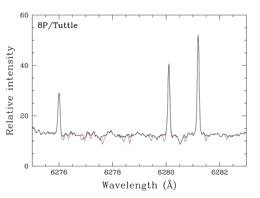
Figure 3: The telluric absorption line correction in the vicinity of the red [OI] lines. The black spectrum has been corrected (thick line), the red one is uncorrected.

The comet Solar continuum has three contributions. First and foremost is the one due to the reflection of sunlight on the dust particles in the coma. Another one appears when the observations are made in or close to the twilight. A third contribution is, in a few cases, the background radiation by the Moon. To remove these contaminations, we Doppler shifted the BASS spectrum to the proper values and scaled the intensities until the solar features are completely removed. This provides the final spectrum such as the one presented in Fig. 4 for comet 8P/Tuttle, free of any solar and telluric lines.

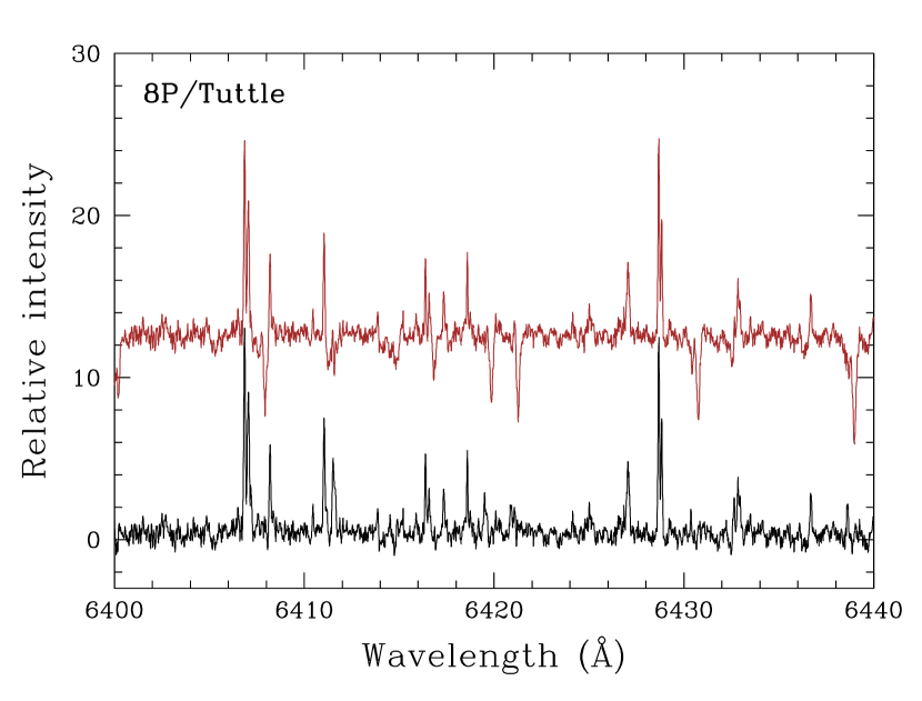
Figure 4: The solar continuum has been removed in the lower spectrum (black) while it is present in the upper one (in red). It corresponds to the final spectrum on which the measurements of the [OI] are made.

4 Data analysis

After the reduction and the correction of the data, we measured both the intensity and the FWHM of the three forbidden oxygen lines by fitting a gaussian profile using the IRAF software. The observed width is the convolution of the instrumental profile with the natural width :

$$\rm{FWHM_{observed}(\lambda)}=\sqrt{\rm{FWHM^{2}_{intrinsic}(\lambda)}+\rm{FWHM^{2}_{instrumental}(\lambda)}}\leavevmode\nobreak\ ,$$ (7)

where the instrumental width corresponds to the width of the Th-Ar lines.

These measurements can only be performed with best accuracy when the cometary oxygen lines are well separated from the telluric [OI] lines, i.e, when the geocentric velocitiy of the comet exceeds 15 km s^-1. Using the deblend function of the splot package in IRAF, we could measure the [OI] lines for Doppler shifts as low as 7 km s^-1.

5 Results

We have measured the two ratios and the FWHM of the three [OI] lines. To reach such goals, a relative calibration using the well known UVES instrumental response curve provided by ESO was enough. Nevertheless, we will investigate how to produce absolute flux calibrated spectra in order to derive production rates of the oxygen parent species in a future work. Therefore, in this current study, the production rates of H₂O to assess the activity of the comet have been taken from literature.

5.1 Intensity ratios

Comet	JD - 2 450 000.5	r (AU)	Intensity (ADU)			$\frac{I_{6300}}{I_{6364}}$	$\frac{I_{5577}}{I_{6300}+I_{6364}}$
			5577.339 Å	6300.304 Å	6363.776 Å
C/2002 V1 (NEAT)	2 647.037	1.22	2348	27539	8875	3.10	0.065
C/2002 V1 (NEAT)	2 647.062	1.22	2255	26790	8875	3.02	0.063
C/2002 V1 (NEAT)	2 649.031	1.18	3220	35672	11704	3.05	0.068
C/2002 V1 (NEAT)	2 649.056	1.18	3137	33738	11105	3.04	0.070
C/2002 V1 (NEAT)	2 719.985	1.01	8657	68162	22381	3.05	0.096
C/2002 X5 (Kudo-Fujikawa)	2 705.017	1.06	4016	31491	10589	2.97	0.095
C/2002 X5 (Kudo-Fujikawa)	2 705.039	1.07	4430	32822	10997	2.98	0.101
C/2002 X5 (Kudo-Fujikawa)	2 705.060	1.07	4249	32510	10816	3.01	0.098
C/2002 Y1 (Juels-Holvorcem)	2 788.395	1.14	6223	50960	17387	2.93	0.091
C/2002 Y1 (Juels-Holvorcem)	2 788.416	1.14	6386	54683	18167	3.01	0.088
C/2002 Y1 (Juels-Holvorcem)	2 789.394	1.16	3942	25792	8659	2.98	0.114
C/2002 Y1 (Juels-Holvorcem)	2 789.415	1.16	4254	31262	10398	3.01	0.102
C/2001 Q4 (NEAT)	2 883.293	3.73	143	324	110	2.95	0.329
C/2001 Q4 (NEAT)	2 883.349	3.73	151	353	110	3.22	0.326
C/2001 Q4 (NEAT)	2 889.236	3.67	-	354	112	3.17	-
C/2001 Q4 (NEAT)	2 889.320	3.66	261	677	193	3.51	0.300
C/2002 T7 (LINEAR)	3 131.421	0.68	116522	642304	211120	3.04	0.137
C/2002 T7 (LINEAR)	3 151.976	0.94	50544	365664	104187	3.51	0.108
C/2002 T7 (LINEAR)	3 152.036	0.94	40165	327184	96554	3.39	0.095
C/2003 K4 (LINEAR)	3 131.342	2.61	464	3609	1172	3.08	0.097
C/2003 K4 (LINEAR)	3 132.343	2.59	561	5027	1607	3.13	0.085
C/2003 K4 (LINEAR)	3 329.344	1.20	9244	94723	29640	3.20	0.074
9P/Tempel 1	3 553.955	1.51	230	3178	1039	3.06	0.054
9P/Tempel 1	3 554.954	1.51	172	3153	1051	3.00	0.041
9P/Tempel 1	3 555.955	1.51	-	3894	1297	3.00	-
9P/Tempel 1	3 557.007	1.51	341	5618	1842	3.05	0.046
9P/Tempel 1	3 557.955	1.51	223	5154	1595	3.23	0.033
9P/Tempel 1	3 558.952	1.51	277	5267	1629	3.23	0.040
9P/Tempel 1	3 559.954	1.51	291	4618	1440	3.21	0.048
9P/Tempel 1	3 560.952	1.51	388	4984	1571	3.17	0.059
9P/Tempel 1	3 561.953	1.51	211	4281	1347	3.18	0.037
9P/Tempel 1	3 562.956	1.51	142	4162	1281	3.25	0.026
73P-C/Schwassmann-Wachmann 3	3 882.367	0.95	16505	115170	35526	3.24	0.110
73P-B/Schwassmann-Wachmann 3	3 898.369	0.94	4890	33987	11226	3.03	0.108
8P/Tuttle	4 481.021	1.04	1779	28517	9385	3.04	0.047
8P/Tuttle	4 493.018	1.03	4437	74360	24565	3.03	0.045
8P/Tuttle	4 500.017	1.03	4179	64979	21424	3.03	0.048
103P/Hartley 2	5 505.288	1.06	45	373	120	3.12	0.092
103P/Hartley 2	5 505.328	1.06	50	456	144	3.22	0.100
103P/Hartley 2	5 510.287	1.07	51	390	121	3.24	0.073
103P/Hartley 2	5 510.328	1.07	41	425	131	3.17	0.083
103P/Hartley 2	5 511.363	1.08	48	395	125	3.17	0.093
C/2009 P1 (Garradd)	5 692.383	3.25	180	652	224	2.92	0.205
C/2009 P1 (Garradd)	5 727.322	2.90	129	693	205	3.38	0.143
C/2009 P1 (Garradd)	5 767.278	2.52	1110	8276	2652	3.12	0.102
C/2009 P1 (Garradd)	5 813.991	2.09	1594	17035	5666	3.01	0.070
C/2009 P1 (Garradd)	5 814.974	2.08	1571	16873	5489	3.07	0.070
C/2009 P1 (Garradd)	5 815.982	2.07	1506	17557	5780	3.04	0.065

Table 4: Intensities given in ADU (Analog-to-Digital Units) and measured line ratios for the three forbidden oxygen lines in the spectra of each comet. For the third spectrum of comets C/2001 Q4 and 9P, the green line could not be measured because of a contamination by a cosmic ray.

Comet	N	$\frac{I_{6300}}{I_{6364}}$	$\frac{I_{5577}}{I_{6300}+I_{6364}}$
C/2002 V1 (NEAT)	5	3.05 $\pm$ 0.03	0.07 $\pm$ 0.01
C/2002 X5 (Kudo-Fujikawa)	3	2.99 $\pm$ 0.02	0.10 $\pm$ 0.003
C/2002 Y1 (Juels-Holvorcem)	4	2.98 $\pm$ 0.04	0.10 $\pm$ 0.01
C/2001 Q4 (NEAT)	4	3.21 $\pm$ 0.23	0.32 $\pm$ 0.02
C/2002 T7 (LINEAR)	3	3.31 $\pm$ 0.18	0.15 $\pm$ 0.05
C/2003 K4 (LINEAR)	3	3.14 $\pm$ 0.06	0.09 $\pm$ 0.01
9P/Tempel 1	10	3.14 $\pm$ 0.10	0.04 $\pm$ 0.01
73P-C/SW 3	1	3.25	0.11
73P-B/SW 3	1	3.03	0.11
8P/Tuttle	3	3.03 $\pm$ 0.01	0.05 $\pm$ 0.01
103P/Hartley 2	5	3.15 $\pm$ 0.07	0.08 $\pm$ 0.02
C/2009 P1 (Garradd)	2	3.15 $\pm$ 0.33	0.017 $\pm$ 0.04
C/2009 P1 (Garradd)	3	3.04 $\pm$ 0.03	0.07 $\pm$ 0.003

Table 5: Average values of the line ratios for each comet. The errors listed are the standard deviation of the N spectra available for each comet. 73P-C/SW3 and 73P-C/SW3 have no error because we obtained only one spectrum for these comets.

The two measured intensity ratios, $I_{6300}/I_{6364}$ and G/R = $I_{5577}/(I_{6300}+I_{6364})$, are displayed for each spectrum in Fig. 5 and Fig. 6 respectively. When the collisional quenching is neglected, the intensity of a line is given by (Festou & Feldman, 1981) :

$$I=\leavevmode\nobreak\ \leavevmode\nobreak\ \tau_{p}^{-1}\leavevmode\nobreak\ \leavevmode\nobreak\ \alpha\leavevmode\nobreak\ \leavevmode\nobreak\ \beta\leavevmode\nobreak\ \leavevmode\nobreak\ N\leavevmode\nobreak\ \leavevmode\nobreak\ \rm{photons}\leavevmode\nobreak\ \rm{cm}^{-2}\leavevmode\nobreak\ \rm{s}^{-1}$$ (8)

where $\tau_{p}$ is the photo-dissociative lifetime of the parent, $\alpha$ is the yield of photo-dissociation, $\beta$ corresponds to the branching ratio for the transition and $N$ is the column density of the parent. Table 4 lists the line intensities $I$ (in ADU) and the ratios for all the spectra. Table 5 shows the standard deviation ($\sigma$) of the ratio for all the spectra of a given comet. Since usually most of the spectra of a same comet are obtained during a short interval of time at similar heliocentric and geocentric distances as well as the same exposure time, the standard deviation of these measurements provides a good estimate of the error. Indeed this error includes the photon noise and errors coming from the telluric absorption and solar continuum corrections.
The red doublet ratio is remarkably similar for all comets. The average value over the whole sample of comets is $3.11\leavevmode\nobreak\ \pm\leavevmode\nobreak\ 0.10$. The error corresponds to the standard deviation ($\sigma$). The ratio is in agreement with the value of $3.09\leavevmode\nobreak\ \pm\leavevmode\nobreak\ 0.12$ obtained by Cochran (2008) from a sample of 8 comets but with a better accuracy. Since both red lines are transitions from the same level to the ground state, $\tau_{p}$, $\alpha$ and $N$ are equal in Eq. (8) and the intensity ratio $I_{6300}/I_{6364}$ is equivalent to the branching ratio $\beta_{6300}/\beta_{6364}$. Our results are indeed in very good agreement with the theoretical value of the branching ratio of $3.096$ computed for the quantum mechanics (Galavis et al., 1997). Storey & Zeippen (2000) published a new theoretical value of $2.997$ taking into account relativistic effects which should be an improvement over previous determinations. Higher value derived from cometary spectra could point a systematic error due to a small blend of the 6300.304 Å [OI] line with an unidentified cometary feature. In order to check if such systematics is present, we first took the average red line ratio of the three comets at large heliocentric distances (C/2001 Q4, C/2003 K4 and C/2009 P1) since most of the fluorescence lines and then their contamination disappear far from the Sun. We obtained an average ratio of 3.13 $\pm$ 0.07. Secondly, we computed the the same ratio but this time for the terrestrial nightglow and found a ratio equal to 3.20 $\pm$ 0.05 obtained again at the largest cometary distances. These measurements remain in better agreement with the Galavis et al. (1997) value but the error are too large to discard Storey & Zeippen (2000) and we cannot exclude a systematic error.

The G/R ratio has an average value of $0.11\leavevmode\nobreak\ \pm\leavevmode\nobreak\ 0.07$ for the complete sample (see Fig. 6).This result is in agreement with the value of $0.09\leavevmode\nobreak\ \pm\leavevmode\nobreak\ 0.01$ found by Cochran (2008). The dispersion is higher because it includes comets at large heliocentric distances which have different G/R ratio. If we take only comets at ¡ $2.5$ AU into account, the average and dispersion are equal to $0.09\pm 0.02$. This leads to the conclusion that H₂O is the main parent molecule producing oxygen atoms according to Bhardwaj & Raghuram (2012) values (Table 1).

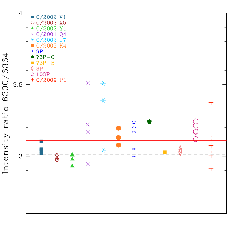
Figure 5: The red doublet ratio for each comet. The spectra of a given comet have the same symbols. The average value of the sample (3.11 $\pm$ 0.10) is shown by the solid line. The dashed lines show the standard deviation ($\sigma$).

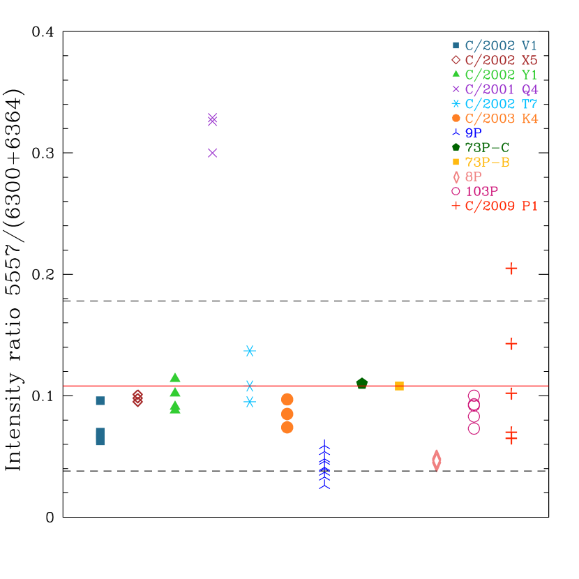
Figure 6: Same figure as Fig. 5 for the G/R ratio. The mean value is 0.11 $\pm$ 0.07. Note the data points for comet Q4 (NEAT) at 3.7 AU.

In order to see if the quenching could play a role on our results, we computed the G/R ratio with respect to the water production rates (Fig. 7). The water production rates of each comet has been compiled from the literature (cf. Table 8). As those comets have been observed in different conditions (of production rates and heliocentric distances), the lack of trend in this analysis suggests that quenching is negligible and does not significantly affect our main conclusions. However, we have started to work on a model based on the Bhardwaj & Raghuram (2012) paper and on Monte Carlo simulations to estimate the quenching. A careful computation of the quenching is not an easy task and we will give our new results, including a detailed discussion of the quenching, in a forthcoming paper.

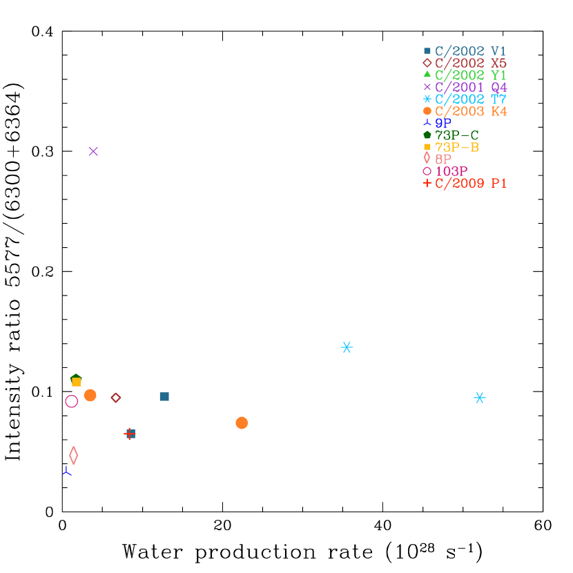
Figure 7: The G/R ratio against the water production rate. No trend appears. This analysis shows that the quenching can be neglected for our study.

5.2 Line widths

Comet	JD - 2 450 000.5	r (AU)	FWHMobserved ($\AA$)			FWHMintrinsic (km s-1)
			5577.339 Å	6300.304 Å	6363.776 Å	5577.339 Å	6300.304 Å	6363.776 Å
C/2002 V1 (NEAT)	2 647.037	1.22	0.092	0.098	0.094	2.08	1.57	1.40
C/2002 V1 (NEAT)	2 647.062	1.22	0.089	0.095	0.095	1.95	1.42	1.44
C/2002 V1 (NEAT)	2 649.031	1.18	0.096	0.096	0.095	2.23	1.45	1.42
C/2002 V1 (NEAT)	2 649.056	1.18	0.093	0.095	0.094	2.11	1.40	1.38
C/2002 V1 (NEAT)	2 719.985	1.01	0.108	0.098	0.096	2.76	1.54	1.49
C/2002 X5 (Kudo-Fujikawa)	2 705.017	1.06	0.104	0.094	0.093	2.64	1.46	1.50
C/2002 X5 (Kudo-Fujikawa)	2 705.039	1.07	0.104	0.095	0.095	2.61	1.54	1.60
C/2002 X5 (Kudo-Fujikawa)	2 705.060	1.07	0.104	0.095	0.094	2.64	1.50	1.54
C/2002 Y1 (Juels-Holvorcem)	2 788.395	1.14	0.106	0.092	0.091	2.88	1.52	1.47
C/2002 Y1 (Juels-Holvorcem)	2 788.416	1.14	0.103	0.092	0.091	2.75	1.54	1.49
C/2002 Y1 (Juels-Holvorcem)	2 789.394	1.16	0.113	0.095	0.094	3.09	1.59	1.57
C/2002 Y1 (Juels-Holvorcem)	2 789.415	1.16	0.112	0.095	0.094	3.03	1.61	1.59
C/2001 Q4 (NEAT)	2 883.293	3.73	0.101	0.116	0.117	2.51	2.39	2.39
C/2001 Q4 (NEAT)	2 883.349	3.73	0.097	0.123	0.125	2.31	2.63	2.69
C/2001 Q4 (NEAT)	2 889.236	3.67	-	0.119	0.121	-	2.49	2.52
C/2001 Q4 (NEAT)	2 889.320	3.66	0.102	0.125	0.117	2.55	2.75	2.36
C/2002 T7 (LINEAR)	3 131.421	0.68	0.115	0.099	0.100	3.12	1.82	1.80
C/2002 T7 (LINEAR)	3 151.976	0.94	0.101	0.089	0.090	2.84	1.70	1.71
C/2002 T7 (LINEAR)	3 152.036	0.94	0.100	0.088	0.090	2.81	1.66	1.72
C/2003 K4 (LINEAR)	3 131.342	2.61	0.131	0.135	0.136	2.51	1.81	1.66
C/2003 K4 (LINEAR)	3 132.343	2.59	0.106	0.108	0.105	2.76	2.12	1.94
C/2003 K4 (LINEAR)	3 329.344	1.20	0.097	0.094	0.096	2.38	1.52	1.52
9P/Tempel 1	3 553.955	1.51	0.110	0.096	0.093	2.91	1.61	1.43
9P/Tempel 1	3 554.954	1.51	0.091	0.095	0.094	2.14	1.59	1.48
9P/Tempel 1	3 555.955	1.51	-	0.094	0.094	-	1.56	1.46
9P/Tempel 1	3 557.007	1.51	0.091	0.095	0.095	2.03	1.55	1.44
9P/Tempel 1	3 557.955	1.51	0.084	0.095	0.095	1.75	1.54	1.47
9P/Tempel 1	3 558.952	1.51	0.084	0.095	0.095	1.79	1.58	1.48
9P/Tempel 1	3 559.954	1.51	0.101	0.101	0.097	2.57	1.84	1.60
9P/Tempel 1	3 560.952	1.51	0.106	0.098	0.096	2.77	1.72	1.52
9P/Tempel 1	3 561.953	1.51	0.087	0.096	0.095	1.92	1.63	1.48
9P/Tempel 1	3 562.956	1.51	0.081	0.096	0.095	1.67	1.61	1.48
73P-C/Schwassmann-Wachmann 3	3 882.367	0.95	0.104	0.106	0.107	2.12	1.31	1.30
73P-B/Schwassmann-Wachmann 3	3 898.369	0.94	0.110	0.108	0.108	2.46	1.54	1.48
8P/Tuttle	4 481.021	1.04	0.091	0.093	0.091	2.16	1.55	1.36
8P/Tuttle	4 493.018	1.03	0.093	0.093	0.092	2.21	1.55	1.41
8P/Tuttle	4 500.017	1.03	0.095	0.093	0.091	2.28	1.47	1.33
103P/Hartley 2	5 505.288	1.06	0.095	0.091	0.097	2.30	1.35	1.29
103P/Hartley 2	5 505.328	1.06	0.090	0.082	0.081	2.31	1.26	1.25
103P/Hartley 2	5 510.287	1.07	0.092	0.081	0.083	2.31	1.26	1.06
103P/Hartley 2	5 510.328	1.07	0.092	0.081	0.079	2.24	1.27	1.17
103P/Hartley 2	5 511.363	1.08	0.090	0.081	0.081	2.19	1.23	1.18
C/2009 P1 (Garradd)	5 692.383	3.25	0.095	0.091	0.097	2.28	1.67	1.87
C/2009 P1 (Garradd)	5 727.322	2.90	0.099	0.083	0.089	2.54	1.27	1.49
C/2009 P1 (Garradd)	5 767.278	2.52	0.090	0.083	0.084	2.19	1.30	1.31
C/2009 P1 (Garradd)	5 813.991	2.09	0.090	0.085	0.087	2.18	1.25	1.33
C/2009 P1 (Garradd)	5 814.974	2.08	0.089	0.086	0.087	2.16	1.33	1.33
C/2009 P1 (Garradd)	5 815.982	2.07	0.090	0.087	0.089	2.21	1.57	1.58

Table 6: Measured observed FWHM ($\AA$) and intrinsic velocity widths (km s^-1) for the three forbidden oxygen lines in the spectra of each comet. For the third spectrum of comets C/2001 Q4 and 9P, the green line could not be used because of the contamination by a strong cosmic ray.

Comet	N	FWHMintrinsic (km s-1)
		5577.339 Å	6300.304 Å	6363.776 Å
C/2002 V1	5	1.48 $\pm$ 0.07	1.43 $\pm$ 0.04	2.22 $\pm$ 0.32
C/2002 X5	3	1.48 $\pm$ 0.07	1.43 $\pm$ 0.04	2.22 $\pm$ 0.32
C/2002 Y1	4	1.57 $\pm$ 0.04	1.53 $\pm$ 0.06	2.94 $\pm$ 0.15
C/2001 Q4	4	2.57 $\pm$ 0.16	2.49 $\pm$ 0.15	2.46 $\pm$ 0.13
C/2002 T7	3	1.77 $\pm$ 0.09	1.72 $\pm$ 0.07	2.47 $\pm$ 0.64
C/2003 K4	3	1.82 $\pm$ 0.30	1.71 $\pm$ 0.21	2.55 $\pm$ 0.19
9P	10	1.62 $\pm$ 0.09	1.48 $\pm$ 0.05	2.23 $\pm$ 0.47
73P-C	1	1.27	1.27	2.13
73P-B	1	1.54	1.47	2.56
8P	3	1.53 $\pm$ 0.05	1.37 $\pm$ 0.04	2.22 $\pm$ 0.06
103P	5	1.28 $\pm$ 0.05	2.00 $\pm$ 0.07	2.15 $\pm$ 0.20
C/2009 P1	2	1.47 $\pm$ 0.29	1.68 $\pm$ 0.27	2.41 $\pm$ 0.19
C/2009 P1	3	1.34 $\pm$ 0.17	1.42 $\pm$ 0.15	2.18 $\pm$ 0.02

Table 7: Average values of the intrinsic line width for each comet. The errors listed are the standard deviation of the N spectra available for each comet. 73P-C/SW3 and 73P-C/SW3 have no error quoted because we obtained only one spectrum for these comets.

Table 6 lists the intrinsic line velocity widths (FWHM$(\rm{v})\leavevmode\nobreak\ (km\leavevmode\nobreak\ s^{-1})$). The FWHM($\rm{v}$) is obtained from the FWHM_intrinsic($\rm{\lambda}$) given in the Eq. 7 using the relation :

$$\rm{FWHM(v)}=\frac{FWHM_{intrinsic}\leavevmode\nobreak\ (\rm{\lambda})\leavevmode\nobreak\ \leavevmode\nobreak\ \^{E}\textnormal{$c$}}{\lambda_{[OI]}\leavevmode\nobreak\ 2\leavevmode\nobreak\ \sqrt{\ln\leavevmode\nobreak\ 2}}\leavevmode\nobreak\ ,$$ (9)

where $\lambda_{[OI]}$ corresponds to the wavelength of the considered oxygen line and $c$ is the speed of light (km s^-1). The error on the [OI] line widths of each comet is given by the standard deviation of the N spectra (cf. Table 7). This error is about $5\%$ for the red lines and $10\%$ for the green line which is fainter. The two red lines widths are equal within the errors (1.61 $\pm$ 0.34 km s^-1 for the $6300\leavevmode\nobreak\ \AA$ line and 1.56 $\pm$ 0.54 km s^-1 for the $6364\leavevmode\nobreak\ \AA$ line) which is not a surprise since both lines are transitions from the O(¹D) state to the ground state (Fig. 8). This result is also consistent with the values of Cochran (2008) (1.22 $\pm$ 0.36 km s^-1). Our mean value of the [OI] cometary green line is wider than the red lines and equal to 2.44 $\pm$ 0.28 km s^-1. This peculiarity was already noticed by Cochran (2008) who found a mean velocity of 2.49 $\pm$ 0.36 km s^-1 in good agreement with our value. Figs. 9, 10 and 11 present the width of the three [OI] cometary lines, the three [OI] telluric lines and the width of some representative neighboring cometary lines for comparison. NH₂ lines in the red region and C₂ lines in the green region. The intrinsic average widths of the cometary NH₂ and C₂ lines are respectively $1.00\pm 0.20$ km s^-1 and $1.28\pm 0.17$ km s^-1 and correspond well to what is expected for the gas expansion velocity in the coma at 1 AU. The ejection velocity due to the extra energy coming from the photo-dissociation of the parent molecule should be represented as the excess velocity resulting from the subtraction of the NH₂ or C₂ cometary lines to the [OI] lines. Considering this, we find an average ejection velocities equal to 0.48 $\pm$ 0.16 km s^-1 for the red lines and 1.17 $\pm$ 0.29 km s^-1 for the green line. This analysis and Fig. 12 show clearly that the [OI] cometary green line is wider than the red lines. This width could be explained if the excess energy for the formation of the O(¹S) state is larger than for the O(¹D) state. Contrary to what is observed, theoretical models using Ly-$\alpha$ photons as excitation source give an excess velocity of 1.6 km  s^-1 for the O(¹S) state and a value of 1.8 km  s^-1 for O(¹D) in the case of water photo-dissociation (Festou, 1981).

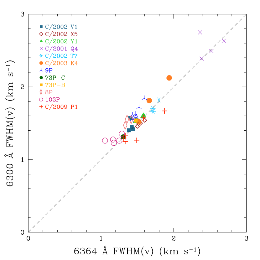
Figure 8: The 6300.304 $\r{A}$ FWHM(v) against the 6363.776 $\r{A}$ one. The different spectra for a given comet are denoted with the same symbol. Note the larger width for C/2001 Q4 (NEAT).

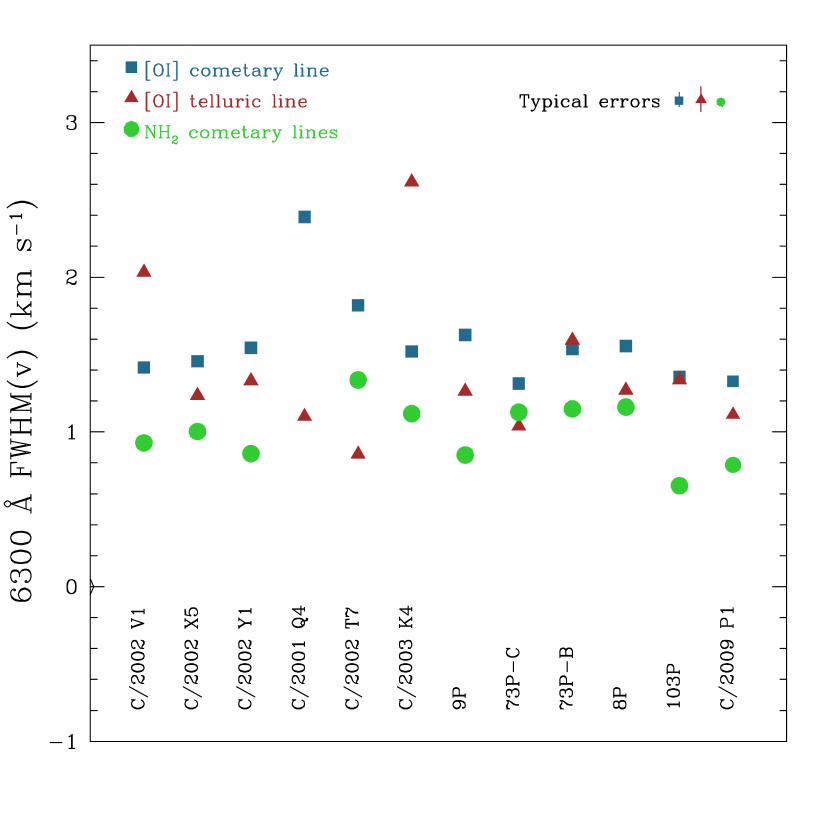
Figure 9: The FWHM(v) of the 6300.304 $\AA$ [OI] cometary line ($\blacksquare$), the [OI] telluric line ($\blacktriangle$) and nearby NH₂ cometary lines ($\CIRCLE$) (km s^-1) for one spectrum per comet. The typical errors correspond to the standard deviation ($\sigma$) obtained considering all the spectra of comet 8P/Tuttle. We have also checked this error by measuring randomly $\sigma$ for a few spectra of other comets. For C/2001 Q4, the NH₂ cometary lines are missing because no fluorescence lines were detected at such large heliocentric distance.

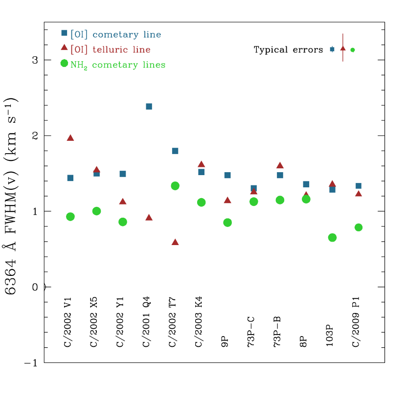
Figure 10: Same figure as Fig. 9 for the 6363.776 $\AA$ line.

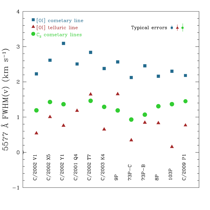
Figure 11: Same figure as Fig. 9 for the 5577.339 $\AA$ line and with C₂ cometary lines. The larger width, by about 1 km s^-1, of the [OI] cometary green line is obvious. It is similar for all comets, C/2001 Q4 included.

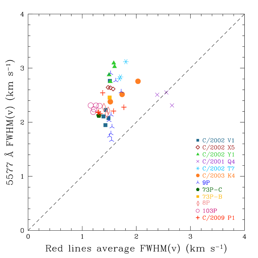
Figure 12: The 5577.339 $\r{A}$ line width against the average width of the red lines. The different spectra of a given comet are denoted with the same symbol. Note that the green line is always larger than the red lines except for C/2001 Q4.

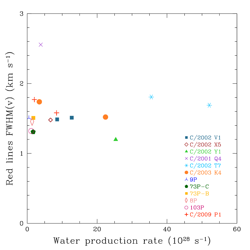
Figure 13: Average of the [OI] red lines FWHM versus the water production rate.

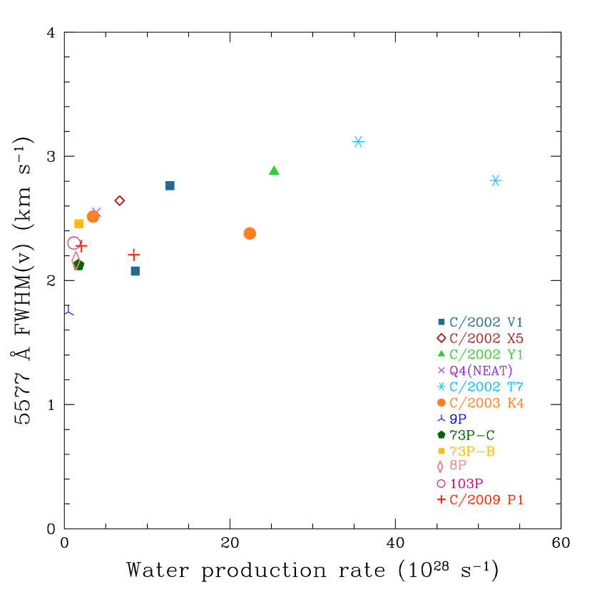
Figure 14: Same figure as Fig. 13 but for the 5577.339 $\r{A}$ line.

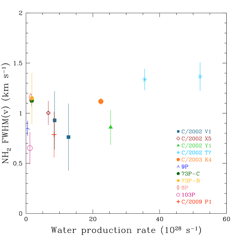
Figure 15: Same figure as Fig. 13 but for the NH₂ line.

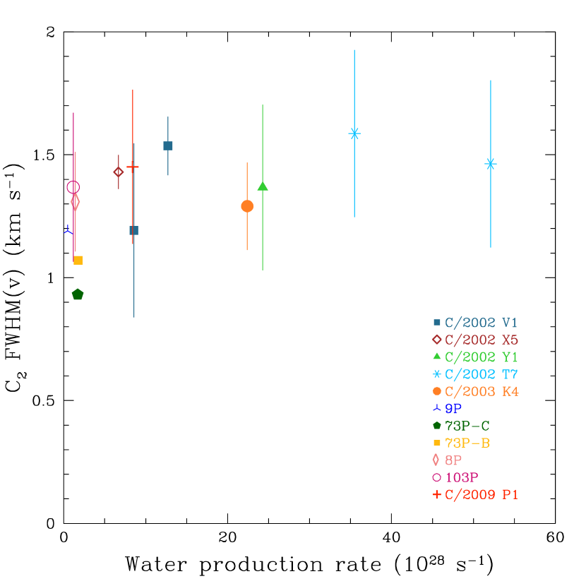
Figure 16: Same figure as Fig. 13 but for the C₂ line.

Comet	$r$	Spectra observed date	$Q_{H_{2}O}$ ($10^{28}$ s-1)	Date	Reference for $Q_{H_{2}O}$
C/2002 V1 (NEAT)	1.22	2003 Jan 8	8.56	2003 Jan 8	Combi et al. (2011)
	1.01	2003 Mar 21	12.73	2003 Mar 21	Combi et al. (2011)
C/2002 X5 (Kudo-Fujikawa)	1.06	2003 Feb 19	6.67	2003 Feb 19	Combi et al. (2011)
C/2002 T7 (LINEAR)	0.68	2004 May 6	35.5	2004 May 5	DiSanti et al. (2006)
	0.94	2004 May 27	52.1	2004 May 27	Combi et al. (2009)
C/2003 K4 (LINEAR)	2.61	2004 May 6	3.47	2004 May 6	(1)
	1.20	2004 Nov 20	22.4	2004 Nov 20	(1)
9P/Tempel 1	1.51	2005 Jul 3	0.47	2005 Jul 3	Gicquel et al. (2012)
73P-C/Schwassmann-Wachmann 3	095	2006 May 27	1.70	2006 May 17	Schleicher & Bair (2011)
73P-B/Schwassmann-Wachmann 3	0.94	2006 Jun 12	1.76	2006 May 18	Schleicher & Bair (2011)
8P/Tuttle	1.04	2008 Jan 16	1.4	2008 Jan 3	Barber et al. (2009)
103P/Hartley 2	1.06	2010 Nov 5	1.15	2010 Nov 31	Knight & Schleicher (2012)
C/2009 P1 (Garradd)	2.07	2011 Sep 12	8.4	2011 Sep 17-21	Paganini et al. (2012)

Table 8: Water production rates and their references. We could find $Q_{H_{2}O}$ data measured very close to our observing dates.
⁽¹⁾ These water production rates were evaluated using the Jorda relation (Jorda et al., 1991) with the magnitudes given by Manfroid et al. (2005).

In Figs. 13 and 14, we compare the velocity of the three oxygen lines and the H₂O production rate from litterature (cf. Table 8). We find that the velocity of the green oxygen line slightly increases with the water production rate. In Fig. 15 and 16, we provide similar plots for the velocities of C₂ and NH₂. The results are in agreement with Tseng et al. (2007) but the error bars are large because the resolution of the spectrometer is at the limit to measure the line broadening and we thus cannot improve their relation.

6 Discussion

6.1 The G/R ratio at large heliocentric distance

In Fig. 6, we noticed that C/2001 Q4 (NEAT) has a G/R ratio of about 0.3 clearly much higher than other comets with values around 0.1. C/2001 Q4 was at 3.7 AU from the Sun and this peculiarity led us to look more carefully on comets observed at large heliocentric distances (Fig. 17) (Decock et al., 2011).

Figure 17: These two hours spectra of comet C/2001 Q4 obtained with the ESO VLT are the most distant detection of [OI] lines in a comet (at 3.7 AU). The lines are well detected and well separated from the telluric line. The width of the green and the red lines are the same.

If we only consider the data taken at $r$ ¡ 2 AU, the G/R ratio average value is equal to 0.09 $\pm$ 0.02 which is in good agreement with the ratio obtained by Bhardwaj & Raghuram (2012) and Festou & Feldman (1981) for H₂O as the parent molecule (see Table 1). The large values of G/R in Q4 (NEAT) at 3.7 AU could be explained by the increasing contribution, at large heliocentric distances, of other parent molecules producing oxygen atoms. It is well known that the sublimation of H₂O significantly decreases beyond 3 AU while the sublimation of other ices like CO and/or CO₂ dominates comet activity (i.e., Crovisier & Encrenaz 2000). In order to investigate this hypothesis, we observed comet C/2009 P1 (Garradd) at four different heliocentric distances from 3.25 AU to 2.07 AU. Fig. 18 presents the G/R intensity ratios as a function of $r$ for all spectra. A relation between the heliocentric distance and the G/R intensity ratio can be seen : the latter is getting rapidly larger when the comet is getting farther from the Sun. We added in this plot the Cochran & Cochran (2001) and Cochran (2008) average values coming from their sample of 8 comets. All these values are clumped around 1 AU with a ratio of $\sim$0.1. C/2001 Q4 is one of their 8 comets and its G/R ratio is $0.09\leavevmode\nobreak\ \pm\leavevmode\nobreak\ 0.02$ at $r=0.98$ AU. A few other measurements found in the literature for comets observed at heliocentric distances beyond 2 AU were also added to the graph. Furusho et al. (2006) used the Subaru telescope to analyse the forbidden oxygen lines in comet 116P/Wild 4 observed at $r\leavevmode\nobreak\ =\leavevmode\nobreak\ 2.4$ AU. Capria et al. (2010) measured the intensity of these lines during and after the outburst of comet 17P/Holmes which occurred on October 24, 2007 when the comet was located at about $r$ = 2.5 AU. McKay et al. (2012b) studied the [OI] lines of the two comets C/2006 W3 Christensen and C/2007 Q3 Siding Spring, respectively at 3.13 and 2.96 AU, with the ARCES echelle spectrometer of 3.5-m telescope at Apache Point Observatory. While the quality of the data are not as good because the lines are faint and sometimes heavily blended with the telluric line, all these measurements show a relatively high value of the G/R ratio when $r$ ¿ 3 AU. This confirms the hypothesis that oxygen is also coming from other molecules. CO and/or CO₂ are obvious candidates as they produce large values of the G/R ratio (see Table 1).

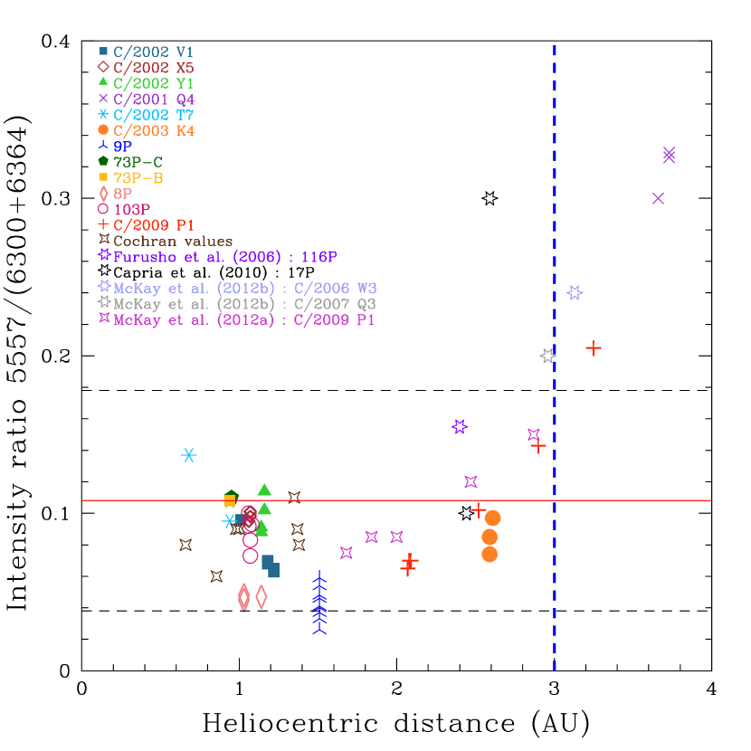
Figure 18: The G/R intensity ratio as a function of the heliocentric distance (AU). The same symbol is used for the different spectra of each comet. The most distant comets have a higher ratio. Other values from the literature are also plotted. The solid line represents the average value only for our sample of spectra and the standard deviation ($\sigma$) range is denoted with horizontal dashed lines. If we only consider the data at $r$ ¡ 2 AU, the average value of G/R ratio is 0.09 $\pm$ 0.02. The vertical dashed line at 3 AU represents the distance out to which the sublimation of water is strongly decreasing (Crovisier & Encrenaz, 2000).

Using HST/STIS observations, Feldman et al. (2004) estimated at 4$\%$ the CO abundance relative to water in comet C/2001 Q4 located at 1 AU from the Sun. The study made by Biver et al. (2012) on comet C/2009 P1 provided an average value of 5$\%$ for the CO abundance when the comet was at 1.9 AU at pre-perihelion phase (October 2011). At large heliocentric distances, CO/H₂O had to be even higher. So the CO molecule could be a candidate to explain such a large G/R ratio. However, Bhardwaj & Raghuram (2012) showed that after the photo-dissociation of H₂O, the next main source for the green line emission is CO₂ with 10-40$\%$ abundance relative to water. They compared their model with the observational values obtained for C/1996 B2 (Hyakutake) by Morrison et al. (1997) and Cochran (2008) when the comet was around 1 AU. Hyakutake is also rich in CO and its abundance was evaluated at 22$\%$ at 1 AU (Biver et al., 1999). Assuming a CO₂ abundance of $1\%$ and a O(¹S) yield of $0.2\%$, Bhardwaj & Raghuram (2012) concluded that the production rates of the O(¹S) are similar for CO and CO₂ ($\sim 10-25\%$) with such abundances. Therefore, since C/2001Q4 and C/2009 P1 have less CO than Hyakutake, CO₂ molecules could rather be the main contributor to the formation of the green line emission for these two comets observed at large heliocentric distance. CO₂ measurements are unfortunately very rare because they are difficult to obtain to confirm this hypothesis. But if this is the case, G/R ratios estimated might be used as a proxy for the CO₂ relative abundance but such a relation should be carefully calibrated on a sample of comets with known CO₂.

Using Eq. 8 and only considering the main parent species of oxygen atoms (i.e H₂O, CO₂ and CO), we can write the G/R ratio as :

$$G/R=\frac{I^{green}}{I^{red}}=\frac{W^{green}_{H_{2}O}\leavevmode\nobreak\ \leavevmode\nobreak\ \beta^{green}\leavevmode\nobreak\ \leavevmode\nobreak\ N_{H_{2}O}+W^{green}_{CO_{2}}\leavevmode\nobreak\ \leavevmode\nobreak\ \beta^{green}\leavevmode\nobreak\ \leavevmode\nobreak\ N_{CO_{2}}+W^{green}_{CO}\leavevmode\nobreak\ \leavevmode\nobreak\ \beta^{green}\leavevmode\nobreak\ \leavevmode\nobreak\ N_{CO}}{W^{red}_{H_{2}O}\leavevmode\nobreak\ \leavevmode\nobreak\ \beta^{red}\leavevmode\nobreak\ \leavevmode\nobreak\ N_{H_{2}O}+W^{red}_{CO_{2}}\leavevmode\nobreak\ \leavevmode\nobreak\ \beta^{red}\leavevmode\nobreak\ \leavevmode\nobreak\ N_{CO_{2}}+W^{red}_{CO}\leavevmode\nobreak\ \leavevmode\nobreak\ \beta^{red}\leavevmode\nobreak\ \leavevmode\nobreak\ N_{CO}}.$$ (10)

where $W^{a}_{b}=\alpha^{a}_{b}\leavevmode\nobreak\ \tau^{-1}_{b}$ corresponds to the effective production rates of O(¹S) and O(¹D) states. However, if we consider that oxygen atoms only come from H₂O and CO molecules, we found that G/R ratio does not change strongly : it varies from 0.08 to 0.1 for a CO abundance between 10$\%$ and 80$\%$. Therefore, we assume that the [OI] atoms are only produced by the H₂O and CO₂ photo-dissociations. Hence, Eq. 10 can be simplified as :

$$G/R=\frac{I^{green}}{I^{red}}=\frac{W^{green}_{H_{2}O}\leavevmode\nobreak\ \leavevmode\nobreak\ \beta^{green}\leavevmode\nobreak\ \leavevmode\nobreak\ N_{H_{2}O}+W^{green}_{CO_{2}}\leavevmode\nobreak\ \leavevmode\nobreak\ \beta^{green}\leavevmode\nobreak\ \leavevmode\nobreak\ N_{CO_{2}}}{W^{red}_{H_{2}O}\leavevmode\nobreak\ \leavevmode\nobreak\ \beta^{red}\leavevmode\nobreak\ \leavevmode\nobreak\ N_{H_{2}O}+W^{red}_{CO_{2}}\leavevmode\nobreak\ \leavevmode\nobreak\ \beta^{red}\leavevmode\nobreak\ \leavevmode\nobreak\ N_{CO_{2}}}$$ (11)

Therefore, the CO₂/H₂O abundance can be computed by :

$$\frac{N_{CO_{2}}}{N_{H_{2}O}}=\frac{(G/R)\leavevmode\nobreak\ W^{red}_{H_{2}O}-\beta^{green}\leavevmode\nobreak\ W^{green}_{H_{2}O}}{\beta^{green}\leavevmode\nobreak\ W^{green}_{CO_{2}}-(G/R)\leavevmode\nobreak\ W^{red}_{CO_{2}}}.$$ (12)

The $W^{a}_{b}$ are independent of the heliocentric distance because all of them depend on the same heliocentric distance. This is also the case for the values given in Table 1. Considering the same values for $W^{a}_{b}$ and $\beta^{green}$, we also computed the CO₂/H₂O abundance from the G/R ratios of comets C/2001 Q4 and C/2009 P1 measured by Cochran (2008) and McKay et al. (2012a), respectively. These results are shown in Fig. 19. We noticed that CO₂/H₂O is as high as 75$\%$ in C/2001 Q4 and that CO₂ starts to contribute to the G/R ratio at 2.5 AU in the comets. This heliocentric distance limit is also shown by Ootsubo et al. (2012) from a sample of 17 comets observed with the AKARI IR space telescope.

Figure 19: Evolution of the CO₂/H₂O abundance as a function of the heliocentric distance (AU). Assuming that a bigger G/R ratio comes from a more important contribution of CO₂ for large heliocentric distance comets, measuring this ratio can give us the CO₂ abundance from ground observations.

Therefore, the forbidden oxygen lines measurement could become a new way to determine the CO₂ abundance in comets at different heliocentric distances from ground observations while the direct measurement of CO₂ molecules is only possible from space.

6.2 The [OI] lines widths

One explanation for the large width of the [OI] green line could be that exciting photons producing oxygen atoms in the ¹S state have more energy than the Lyman $\alpha$ photons and/or come from an other parent molecule. Indeed, Fig. 7 of Bhardwaj & Raghuram (2012) shows that the wavelength region for the major production of O(¹S) coming from CO₂ seems to be the 955-1165 Å band. New theoretical studies could be necessary to evaluate the excess velocity for the O(¹S) state coming from the photo-dissociations of both H₂O and CO₂.
In Fig. 12, we also notice that the [OI] red lines of the comet C/2001 Q4 are wider than in other comets while the width of the green line is normal with respect to other comets. This peculiarity seems real as both red lines show the same width and they are 2-$\sigma$ away from the average value of the sample (1.58 $\pm$ 0.30 km s^-1). The telluric lines in C/2001 Q4 have the usual width (0.99 $\pm$ 0.10 km s^-1 for the 6300 $\AA$ line, 0.87 $\pm$ 0.04 km s^-1 for the 6364 $\AA$ line and 0.80 $\pm$ 0.26 km s^-1 for the green line), excluding a problem with the spectra or the analysis. The width of the red lines and the green line is similar in this only case (2.57 $\pm$ 0.16 km s^-1 for the 6300 $\AA$ line, 2.49 $\pm$ 0.15 km s^-1 for the 6364 $\AA$ and 2.46 $\pm$ 0.13 km s^-1 for the 5577 $\AA$ line) and could give us clues about the process at play. As previously discussed, at large heliocentric distances, the [OI] lines could mainly come from the CO₂ molecules which preferentially photo-dissociate in the ¹S state while at low heliocentric distances, they essentially come from H₂O which preferentially dissociates in the ¹D state (Table 1). This means that at large distances, the red lines are mainly produced through the ¹S-¹D channel together with the green line, while at low distances as H₂O dominates they are mostly produced directly from the ¹D state. We thus expect the widths of the red and green lines to be similar at high distances because the O(¹S) and O(¹D) atoms are mostly produced from a same molecule, while they can differ at low distances, as observed. CO₂ is the best candidate and the larger width could be explained by the main excitation source of CO₂, the 955-1165 $\AA$ band, which is more energetic than Ly-$\alpha$ photons, as shown in Fig. 11 of Bhardwaj & Raghuram (2012). This particularity is not seen for comet C/2009 P1 (Garradd) maybe because the spectrum is not taken at sufficiently large heliocentric distance and the CO₂ abundance was lower than in C/2001 Q4 (NEAT). Anyway, this hypothesis needs to be confirmed by observing other comets at large heliocentric distances (¿ $3.5$ AU).

6.3 103P/Hartley 2

JD - 2 450 000.5	r(AU)	G/R	$N_{CO_{2}}/N_{H_{2}O}$
5 505.288	1.06	0.09	0.028
5 505.328	1.06	0.10	0.040
5 510.287	1.07	0.07	0.001
5 510.328	1.07	0.08	0.015
5 511.363	1.08	0.09	0.030

Table 9: The CO₂/H₂O abundances estimated from Eq. 12 for the comet 103P/Hartley 2.

The Jupiter Family comet 103P/Hartley 2 has been found poor in CO (Weaver et al., 2011) and rich in CO₂ with an CO₂ abundance of $\sim 20\%$ relative to the water from EPOXI measurements (A’Hearn et al., 2011) and with an abundance of $\sim 10\%$ from the ISO observations (Crovisier et al., 1999). Thanks to Eq. 12, we could evaluate the CO₂ abundances from our G/R ratios measured at $\sim 1$ AU and compare them with the values obtained by EPOXI and ISO observations. The results are given in Table 9. The mean G/R ratio of $0.09\leavevmode\nobreak\ \pm\leavevmode\nobreak\ 0.01$ is similar to those of other comets observed below 2.5 AU and give a relative abundance of CO₂ of only $\sim 3\%$ while a G/R ratio of $\sim 0.1$ to $0.2$ would be needed to reach a CO₂ abundance as high as $\sim 10\%$ to $20\%$.
We do not confirm a high value of CO₂ abundance for 103P/Hartley 2 as claimed by (McKay et al., 2012) or a large dispersion in the abundances. Their values might be higher because they used a $W^{green}_{H_{2}O}$ of Bhardwaj & Raghuram (2012) equal to 2.6 10^-8 s^-1 while the value provided in Table 1 of this paper is 6.4 10^-8 s^-1.
The discrepancy with the EPOXI and ISO observations CO₂ abundance is interesting. Below 2.5 AU, G/R values are distributed from 0.05 for comets like 9P/Tempel 1 and 8P/Tuttle and can go up to 0.12 for C/2002 T7 (LINEAR). The spread from comet to comet is higher than the errors estimated from the dispersion from the spectra of a same comet which could be explained by an intrinsic variation of G/R from comet to comet due to the content of CO₂. The G/R range, of the order of 0.1 (implying a CO₂ variation of $\sim 20\%$) is of the same order as the range of CO₂ abundance in comets of various origins measured below 2.5 AU (A’Hearn, 2012).

The fact that some comets, like 9P/Tempel 1 and 8P/Tuttle, have values lower than the pure water case (giving a G/R_min = 0.08 from Bhardwaj & Raghuram (2012)) and that the 103P/Harley 2 G/R ratio is too low compared to EPOXI CO₂ abundances, could indicate a problem with the models. The pure water ratio should be 0.05 or lower based on the comets with the smallest values (9P/Tempel 1 has a CO₂ abundance of $\sim 7\%$ (Feaga et al. (2007a), Feaga et al. (2007b)). Bhardwaj & Raghuram (2012) tried $\alpha^{green}_{H_{2}O}$ values from $0\%$ to $1\%$ and finally chose $1\%$, but this value is uncertain. Without CO₂, G/R_min = $\beta^{green}\leavevmode\nobreak\ W^{green}_{H_{2}O}\leavevmode\nobreak\ /\leavevmode\nobreak\ W^{red}_{H_{2}O}$. If we use $0.5\%$ for $\alpha^{green}_{H_{2}O}$, G/R_min is equal to 0.04 instead of 0.08 which would be in better agreement with our smallest values.

6.4 Deep Impact

The spectra of comet 9P/Tempel 1 were analysed before and after the July 4 collision with the Deep Impact spacecraft. No difference was observed in the intensity ratios and the lines widths before and after the impact (Fig. 20). We have no spectrum during the impact. The first spectrum after the impact was taken at 2453559.954 UT (i.e. $\sim$6 hours after the impact). Cochran (2008) did not notice any change during the impact either.

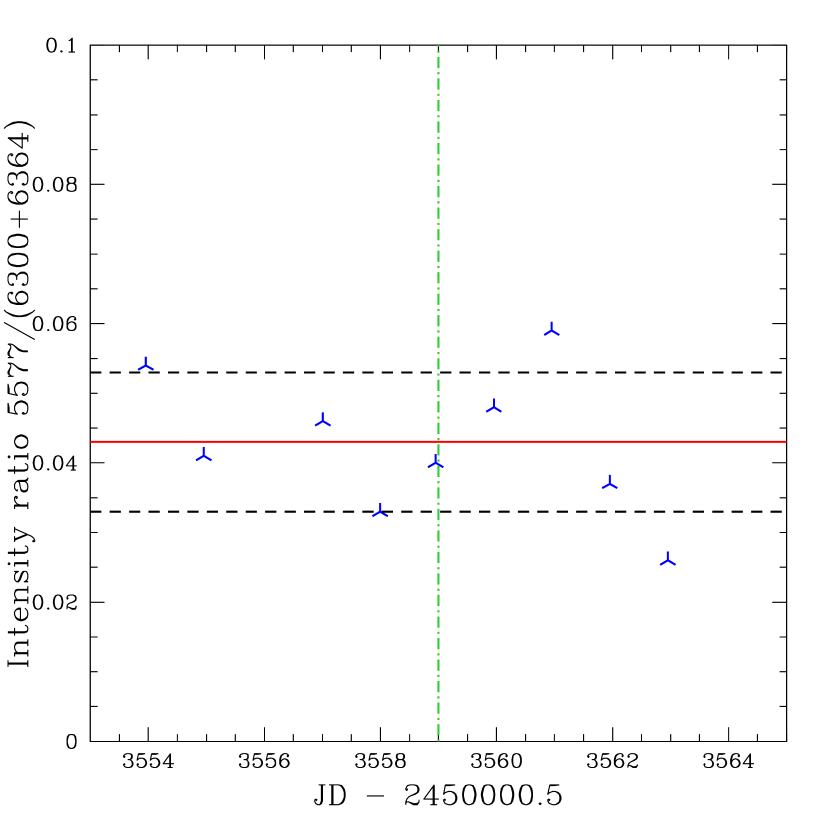
Figure 20: The G/R intensity ratio of comet 9P/Tempel 1 from JD $2453553.955$ to $2453562.956$ UT. The Deep Impact event corresponds to the vertical line (53559 UT). The average value is shown by the solid red line and the dashed lines correspond to the standard deviation ($\sigma$). The mean value around the impact (from 2453553.955 UT to 2453562.956 UT) is $0.04\leavevmode\nobreak\ \pm\leavevmode\nobreak\ 0.01$. No variation of the ratio was noticed after the impact.

6.5 Solar activity

Our data were obtained over the 23^th solar cycle characterized by its maximum of activity in 2001 and its minimum activity in 2008. Despite the decrease of the solar activity during the observations of C/2001 V1 (NEAT) and 8P/Tuttle, no change in the intensities and widths of lines were noticed. The solar activity does not appear to have any influence on the results of our work.

7 Conclusion

From January 2003 to September 2011, 12 comets of various origins were observed at different heliocentric distances and 48 high resolution spectra were obtained with the UVES spectrograph at VLT (ESO). Within this whole sample, we observed the three [OI] forbidden oxygen lines with high resolution and signal-to-noise and we measured the intensity ratios ($I_{6300}/I_{6364}$ and G/R = $I_{5577}$/($I_{6300}+I_{6364}$)) as well as the FWHM (v) of the lines. The results can be summarized as follows :

1. The $I_{6300}/I_{6364}$ ratio (3.11 $\pm$ 0.10) is in very good agreement with the branching ratio obtained by quantum mechanics, especially the work done by Galavis et al. (1997). However, some systematic errors of the order of 0.1 are possible so that we cannot exclude the new value of Storey & Zeippen (2000).

2. From theoretical values given in Table 1, the G/R ratio for comets observed below 2 AU (0.09 $\pm$ 0.02) confirms H₂O as the main parent molecule photo-dissociating to produce oxygen atoms. However, when the comet is located at larger heliocentric distances ($r$ $\geq$ 2.5 AU), the ratio increases rapidly showing that an other parent molecule is contributing. We have shown that CO₂ is the best candidate. Measuring the G/R ratios could then be a new way to estimate the abundances of CO₂, a very difficult task from the ground. Assuming that only the photo-dissociation of H₂O and CO₂ produce [OI], we found a relation between CO₂ abundance and the heliocentric distance of the comet. The C/2001 Q4 (NEAT) abundance of CO₂ at 3.7 AU is found to be $\sim$75$\%$.

3. The intrinsic green line width is wider than the red ones by about 1 km s^-1. Theoretical estimations considering Ly-$\alpha$ as the only excitation source for the two states lead to the conclusion that the excess energy for O(¹D) is larger than for O(¹S) which is in contradiction with our observations. This discrepancy might be explained by a different nature of the excitation source and/or a contribution of CO₂ as parent molecule to the O(¹S) state. Indeed, Bhardwaj & Raghuram (2012) have shown that for the photo-dissociation of CO₂, the main excitation source might rather be the 995-1165 $\r{A}$ band. To check this hypothesis quantitatively, it would be necessary to estimate theoretically the excess energy for the oxygen atoms when the wavelength band is 995-1165 Å, accounting for the photo-dissociation of both H₂O and CO₂. The widths of the three [OI] lines are similar in C/2001 Q4 at $\sim$ 3.7 AU. This could be in agreement with CO₂ being the main contributor for the three [OI] lines at large heliocentric distance. Other comets at large $r$ have to be observed to test this hypothesis.

4. More CO₂ (and CO) abundance determinations, together with G/R oxygen ratios and line widths at different heliocentric distances, are clearly needed in order to give a general conclusion about the oxygen parent molecule.

5. The CO₂ rich comet 103P/Hartley 2 ($\sim 20\%$) does not present a high G/R ratio normally expected from Eq. 12. We suggest a new value of $0.5\%$ for $\alpha^{green}_{H_{2}O}$ that could also explain the low values of G/R obtained for comets 9P/Tempel 1 and 8P/Tuttle.

References

- A’Hearn (2012) A’Hearn, M. F. 2012, in American Astronomical Society Meeting Abstracts, Vol. 220, American Astronomical Society Meeting Abstracts 220, 120.04
- A’Hearn et al. (2011) A’Hearn, M. F., Belton, M. J. S., Delamere, W. A., et al. 2011, Science, 332, 1396
- Barber et al. (2009) Barber, R. J., Miller, S., Dello Russo, N., et al. 2009, MNRAS, 398, 1593
- Bhardwaj & Raghuram (2012) Bhardwaj, A. & Raghuram, S. 2012, ApJ, 748, 13
- Biver et al. (1999) Biver, N., Bockelée-Morvan, D., Crovisier, J., et al. 1999, AJ, 118, 1850
- Biver et al. (2012) Biver, N., Bockelée-Morvan, D., Lis, D. C., et al. 2012, LPI Contributions, 1667, 6330
- Capria et al. (2010) Capria, M. T., Cremonese, G., & de Sanctis, M. C. 2010, A&A, 522, A82
- Cochran (2008) Cochran, A. L. 2008, Icarus, 198, 181
- Cochran & Cochran (2001) Cochran, A. L. & Cochran, W. D. 2001, Icarus, 154, 381
- Combi et al. (2011) Combi, M. R., Boyd, Z., Lee, Y., et al. 2011, Icarus, 216, 449
- Combi et al. (2009) Combi, M. R., Mäkinen, J. T. T., Bertaux, J.-L., Lee, Y., & Quémerais, E. 2009, AJ, 137, 4734
- Crovisier & Encrenaz (2000) Crovisier, J. & Encrenaz, T., eds. 2000, Comet science : the study of remnants from the birth of the solar system
- Crovisier et al. (1999) Crovisier, J., Encrenaz, T., Lellouch, E., et al. 1999, in ESA Special Publication, Vol. 427, The Universe as Seen by ISO, ed. P. Cox & M. Kessler, 161
- Decock et al. (2011) Decock, A., Jehin, E., Manfroid, J., & Hutsemékers, D. 2011, in EPSC-DPS Joint Meeting 2011, 1126
- Dekker et al. (2000) Dekker, H., D’Odorico, S., Kaufer, A., Delabre, B., & Kotzlowski, H. 2000, in Presented at the Society of Photo-Optical Instrumentation Engineers (SPIE) Conference, Vol. 4008, Society of Photo-Optical Instrumentation Engineers (SPIE) Conference Series, ed. M. Iye & A. F. Moorwood, 534–545
- DiSanti et al. (2006) DiSanti, M. A., Bonev, B. P., Magee-Sauer, K., et al. 2006, ApJ, 650, 470
- Ehrenfreund & Charnley (2000) Ehrenfreund, P. & Charnley, S. B. 2000, ARA&A, 38, 427
- Feaga et al. (2007a) Feaga, L. M., A’Hearn, M. F., Sunshine, J. M., Groussin, O., & Farnham, T. L. 2007a, Icarus, 190, 345
- Feaga et al. (2007b) Feaga, L. M., A’Hearn, M. F., Sunshine, J. M., Groussin, O., & Farnham, T. L. 2007b, Icarus, 191, 134
- Feldman et al. (2004) Feldman, P. D., Weaver, H. A., Christian, D., et al. 2004, in Bulletin of the American Astronomical Society, Vol. 36, AAS/Division for Planetary Sciences Meeting Abstracts 36, 1121
- Festou & Feldman (1981) Festou, M. & Feldman, P. D. 1981, A&A, 103, 154
- Festou (1981) Festou, M. C. 1981, A&A, 96, 52
- Furusho et al. (2006) Furusho, R., Kawakita, H., Fuse, T., & Watanabe, J. 2006, Advances in Space Research, 38, 1983
- Galavis et al. (1997) Galavis, M. E., Mendoza, C., & Zeippen, C. J. 1997, A&AS, 123, 159
- Gicquel et al. (2012) Gicquel, A., Bockelée-Morvan, D., Zakharov, V. V., et al. 2012, A&A, 542, A119
- Huebner & Carpenter (1979) Huebner, W. F. & Carpenter, C. W. 1979, NASA STI/Recon Technical Report N, 80, 24243
- Jehin et al. (2009) Jehin, E., Manfroid, J., Hutsemékers, D., Arpigny, C., & Zucconi, J.-M. 2009, Earth Moon and Planets, 105, 167
- Jorda et al. (1991) Jorda, L., Crovisier, J., & Green, D. W. E. 1991, LPI Contributions, 765, 108
- Knight & Schleicher (2012) Knight, M. M. & Schleicher, D. G. 2012, ArXiv e-prints
- Levison (1996) Levison, H. F. 1996, in Astronomical Society of the Pacific Conference Series, Vol. 107, Completing the Inventory of the Solar System, ed. T. Rettig & J. M. Hahn, 173–191
- Manfroid et al. (2005) Manfroid, J., Jehin, E., Hutsemékers, D., et al. 2005, A&A, 432, L5
- Manfroid et al. (2009) Manfroid, J., Jehin, E., Hutsemékers, D., et al. 2009, A&A, 503, 613
- McKay et al. (2012a) McKay, A. J., Chanover, N. J., DiSanti, M. A., et al. 2012a, LPI Contributions, 1667, 6212
- McKay et al. (2012b) McKay, A. J., Chanover, N. J., Morgenthaler, J. P., et al. 2012b, Icarus, 220, 277
- McKay et al. (2012) McKay, A. J., Chanover, N. J., Morgenthaler, J. P., et al. 2012, Icarus, http://dx.doi.org/10.1016/j.icarus.2012.06.020, in press
- Morrison et al. (1997) Morrison, N. D., Knauth, D. C., Mulliss, C. L., & Lee, W. 1997, PASP, 109, 676
- Ootsubo et al. (2012) Ootsubo, T., Kawakita, H., Hamada, S., et al. 2012, ApJ, 752, 15
- Paganini et al. (2012) Paganini, L., Mumma, M. J., Villanueva, G. L., et al. 2012, ApJ, 748, L13
- Schleicher & Bair (2011) Schleicher, D. G. & Bair, A. N. 2011, AJ, 141, 177
- Slanger et al. (2006) Slanger, T. G., Cosby, P. C., Sharpee, B. D., Minschwaner, K. R., & Siskind, D. E. 2006, Journal of Geophysical Research (Space Physics), 111, 12318
- Storey & Zeippen (2000) Storey, P. J. & Zeippen, C. J. 2000, MNRAS, 312, 813
- Swings (1962) Swings, P. 1962, Annales d’Astrophysique, 25, 165
- Tseng et al. (2007) Tseng, W.-L., Bockelée-Morvan, D., Crovisier, J., Colom, P., & Ip, W.-H. 2007, A&A, 467, 729
- Weaver et al. (2011) Weaver, H. A., Feldman, P. D., A’Hearn, M. F., Dello Russo, N., & Stern, S. A. 2011, ApJ, 734, L5