Fundamental Properties of Stars using Asteroseismology from KEPLER & CoRoT and Interferometry from the CHARA Array

Abstract

We present results of a long-baseline interferometry campaign using the PAVO beam combiner at the CHARA Array to measure the angular sizes of five main-sequence stars, one subgiant and four red giant stars for which solar-like oscillations have been detected by either Kepler or CoRoT. By combining interferometric angular diameters, Hipparcos parallaxes, asteroseismic densities, bolometric fluxes and high-resolution spectroscopy we derive a full set of near model-independent fundamental properties for the sample. We first use these properties to test asteroseismic scaling relations for the frequency of maximum power ($\nu_{\rm max}$) and the large frequency separation ($\Delta\nu$). We find excellent agreement within the observational uncertainties, and empirically show that simple estimates of asteroseismic radii for main-sequence stars are accurate to $\lesssim 4\%$. We furthermore find good agreement of our measured effective temperatures with spectroscopic and photometric estimates with mean deviations for stars between $T_{\rm eff}=4600-6200$ K of $-22\pm 32$ K (with a scatter of 97 K) and $-58\pm 31$ K (with a scatter of 93 K), respectively. Finally we present a first comparison with evolutionary models, and find differences between observed and theoretical properties for the metal-rich main-sequence star HD 173701. We conclude that the constraints presented in this study will have strong potential for testing stellar model physics, in particular when combined with detailed modelling of individual oscillation frequencies.

1. Introduction

The knowledge of fundamental properties such as temperature, radius and mass of stars in different evolutionary phases plays a key role in many applications of modern astrophysics. Examples include the improvement of model physics of stellar structure and evolution such as convection (see, e.g. Demarque et al., 1986; Monteiro et al., 1996; Deheuvels & Michel, 2011; Trampedach & Stein, 2011; Piau et al., 2011), the calibration of empirical relations such as the color-temperature scale for cool stars (see, e.g., Flower, 1996; Ramírez & Meléndez, 2005; Casagrande et al., 2010), and the characterization of physical properties and habitable zones of exoplanets (see, e.g., Baines et al., 2008; van Belle & von Braun, 2009; von Braun et al., 2011a, b).

Many methods to determine properties of single field stars are indirect, and therefore of limited use for improving stellar models. Asteroseismology, the study of stellar oscillations, is a powerful method to determine properties of solar-type stars such as the mean stellar density with little model dependence (see, e.g., Brown & Gilliland, 1994; Christensen-Dalsgaard, 2004; Aerts et al., 2010). Additionally, long-baseline interferometry can be used to measure the angular sizes of stars which, in combination with a parallax, yields a linear radius and, when combined with an estimate for the bolometric flux, provides a direct measurement of a star’s effective temperature (see, e.g., Code et al., 1976; Boyajian et al., 2009; Baines et al., 2009; Boyajian et al., 2012a, b; Creevey et al., 2012). Therefore, the combination of both methods in principle allows a determination of radii, masses and temperatures of stars with little model dependence.

While the potential of combining asteroseismology and interferometry has been long recognized (see, e.g, Cunha et al., 2007), observational constraints have so far restricted an application for cool stars to relatively few bright objects (North et al., 2007; Bruntt et al., 2010; Bazot et al., 2011). Recent technological advances, however, have changed this picture. The launches of the space telescopes CoRoT (Convection, Rotation and planetary Transits, Baglin et al., 2006a, b) and Kepler (Borucki et al., 2010; Koch et al., 2010) has increased the number of stars with detected solar-like oscillations to several thousands, providing a large sample spanning from the main-sequence to He-core burning red giant stars (De Ridder et al., 2009; Hekker et al., 2009; Gilliland et al., 2010b; Chaplin et al., 2011). At the same time, the development of highly sensitive instruments such as the PAVO beam combiner (Ireland et al., 2008) at the CHARA Array (ten Brummelaar et al., 2005) have pushed the sensitivity limits of long-baseline interferometry, bringing into reach the brightest objects for which high-quality space-based asteroseismic data are available. Using these recent advances, we present a systematic combined asteroseismic and interferometric study of low-mass stars spanning from the main-sequence to the red clump.

2. Target Sample

Our target sample was selected to optimize the combination of asteroseismology and interferometry given the observational constraints, while also covering a large parameter space in stellar evolution. The majority of our stars were taken from the sample analyzed by the Kepler Asteroseismic Science Consortium (KASC). We selected four unevolved stars, which are among the brightest oscillating solar-type stars observed by Kepler. Note that our interferometric results for $\theta$ Cyg (Guzik et al., 2011) and 16 Cyg A&B (Metcalfe et al., 2012) will be presented elsewhere. For the Kepler giant sample, four of the brightest red giants with the best Hipparcos parallaxes were selected. Finally, the main-sequence stars HD 175726 and HD 181420 in our sample are located in the CoRoT field towards the galactic center, and were among the first CoRoT main-sequence stars with detected oscillations (Barban et al., 2009; Mosser et al., 2009). Note that our PAVO campaign is also targeting solar-type oscillators in the CoRoT field in the galactic anti-center, such as the F-star HD 49933 (Appourchaux et al., 2008; Benomar et al., 2009; Kallinger et al., 2010a), which has already been subject to interferometric follow-up (Bigot et al., 2011). However, due to poor weather conditions during the winter seasons on Mt. Wilson, not enough data has yet been collected for these targets.

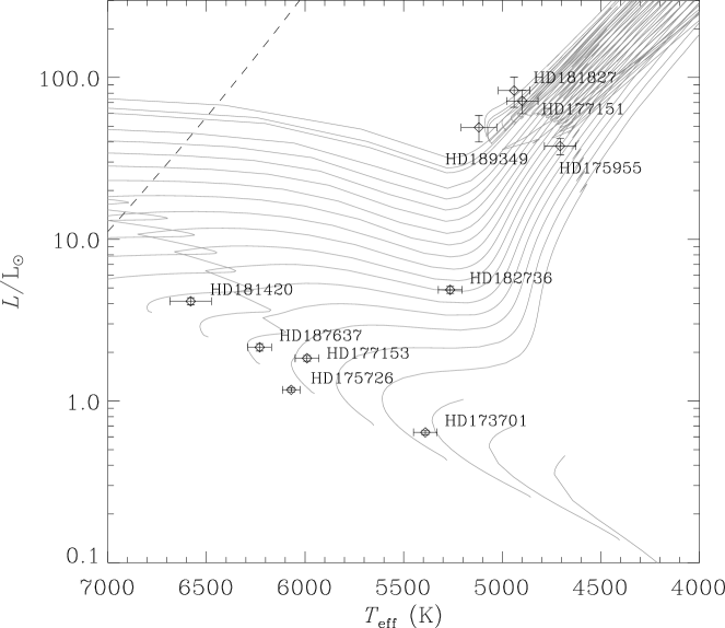
Figure 1.— H-R diagram with the position of the target stars calculated using spectroscopy, photometry and Hipparcos parallaxes. Solar metallicity BaSTI evolutionary tracks from 0.6-2.6 $M_{\sun}$ in steps of 0.1 $M_{\sun}$ are shown as grey lines. The dashed line marks the approximate location of the cool edge of the instability strip.

In the remainder of this section we summarize the basic parameters of our target stars derived using classical methods and measurements available in the literature. Table 1 lists the complete target sample of our study, with spectral types taken from the HD catalog. Nine of the ten stars in our sample have atmospheric parameters derived from modeling several hundred lines in high-resolution spectra using the VWA package (Bruntt et al., 2010), as presented by Bruntt (2009), Bruntt et al. (2012) and Thygesen et al. (2012). These are also listed in Table 1. For HD 189349, we have analyzed a spectrum obtained with the NARVAL spectrograph at the Pic du Midi Observatory using three different methods: VWA (Bruntt et al., 2010), ROTFIT (Frasca et al., 2003, 2006) and the method described by Santos et al. (2004), Sousa et al. (2006) and Sousa et al. (2008). In two of the three methods the surface gravity was fixed to the value calculated from asteroseismic scaling relations (see next section). The resulting spectroscopic parameters for each method are listed in Table 2, and we have adopted a weighted mean of all three methods, given in Table 1, for the remainder of this paper. Note that for HD 173701 spectroscopic parameters have also been published by Valenti & Fischer (2005), Mishenina et al. (2004) and Kovtyukh et al. (2003), which are also listed in Table 2 for comparison. The published values are in good agreement with the values adopted here.

Table 1Fundamental properties of target stars using available literature information. Stars are separated into main-sequence and subgiant stars (top) and red giants (bottom).

HD	KIC	Sp.T.	$V$	$B-V$	Spectroscopy			Hipparcos
					$T_{\rm eff}$	$\log g$	[Fe/H]	$\pi$ (mas)	$L/L_{\sun}$
1737011	8006161	K0V	$7.514$	$0.878$	5390(60)	4.49(3)	$+0.34$(6)	37.47(49)	0.64(2)
1757262	–	G5V	$6.711$	$0.571$	6070(45)	4.53(4)	$-0.07$(3)	37.73(51)	1.17(4)
1771531	6106415	G0V	$7.205$	$0.558$	5990(60)	4.31(3)	$-0.09$(6)	24.11(44)	1.84(7)
1814202	–	F2V	$6.561$	$0.434$	6580(105)	4.26(8)	$+0.00$(6)	21.05(48)	4.1(2)
1827361	8751420	G0IV	$7.022$	$0.800$	5264(60)	3.70(3)	$-0.15$(6)	17.35(41)	4.9(2)
1876371	6225718	F5V	$7.520$	$0.500$	6230(60)	4.32(3)	$-0.17$(6)	19.03(46)	2.1(1)
1759553	10323222	K0III	$7.014$	$1.171$	4706(80)	2.60(1)	$+0.06$(15)	7.62(38)	38(4)
1771513	10716853	K0III	$7.040$	$0.994$	4898(80)	2.62(1)	$-0.10$(15)	4.92(38)	72(12)
1818273	8813946	K0III	$7.188$	$1.012$	4940(80)	2.81(1)	$+0.14$(15)	4.23(43)	83(18)
189349	5737655	G5III	$7.305$	$0.878$	5118(90)	2.4(1)	$-0.56$(16)	5.32(47)	49(9)

All stars in our sample have measured Hipparcos parallaxes (van Leeuwen, 2007), with uncertainties ranging from $\sim$ 1 to 10 %. All unevolved stars in our sample are at distances $<60$ pc and hence reddening is expected to be negligible (see Molenda-Żakowicz et al., 2009; Bruntt et al., 2012). Hence, we assumed zero reddening for all unevolved stars with an uncertainty of 0.005 mag. For the giants, we have estimated reddening by comparing observed colors to synthetic photometry of models matching the spectroscopic parameters in Table 1, as described in more detail in Section 3.3. To estimate an uncertainty, we have compared these values to $E(B-V)$ values listed in the Kepler Input Catalog (KIC, Brown et al., 2011) for nearby stars and to estimates from the 3-D extinction model by Drimmel et al. (2003). The mean scatter between these methods for all stars is 0.02 mag, which we adopt as our uncertainty in $E(B-V)$ for the giants in our sample. Finally, we used the spectroscopically determined effective temperatures and metallicities to estimate a bolometric correction for each star using the calibrations by Flower (1996) and Alonso et al. (1999) with appropriate zero-points as discussed in Torres (2010), yielding the stellar luminosity given in the last column of Table 1. Figure 1 shows an H-R diagram of our target stars, according to the properties listed in Table 1, together with solar-metallicity BaSTI evolutionary tracks (Pietrinferni et al., 2004).

Table 2Atmospheric parameters for stars from different methods.

HD	KIC	$T_{\rm eff}$	$\log g$	[Fe/H]	Ref
173701	8006161	5390(60)	4.49(3)	0.34(6)	1∗
		5399(44)	4.53(6)	0.32(3)	2
		5423(20)	4.4(2)	0.2(1)	3
		5423(10)	–	–	4
189349	5737655	5070(100)	2.4(1)	-0.7(1)	5a∗
		5145(63)	2.4(1)	-0.54(5)	5b∗
		5163(71)	2.9(2)	-0.44(11)	5c

3. Observations

3.1. Asteroseismology

The asteroseismic results presented in this paper are based on observations obtained by the Kepler and CoRoT space telescopes. Both satellites deliver near-uninterrupted, high S/N time series which are ideally suited for asteroseismic studies. In this paper, we focus on two global parameters: the frequency of maximum power ($\nu_{\rm max}$) and the large frequency separation ($\Delta\nu$). These are frequently used to determine fundamental properties of main-sequence and red giant stars (see, e.g., Stello et al., 2009b; Kallinger et al., 2010b, c; Chaplin et al., 2011; Hekker et al., 2011a, b; Silva Aguirre et al., 2011; Huber et al., 2011). For a general introduction to solar-like oscillations, we refer the reader to the review by Bedding (2011).

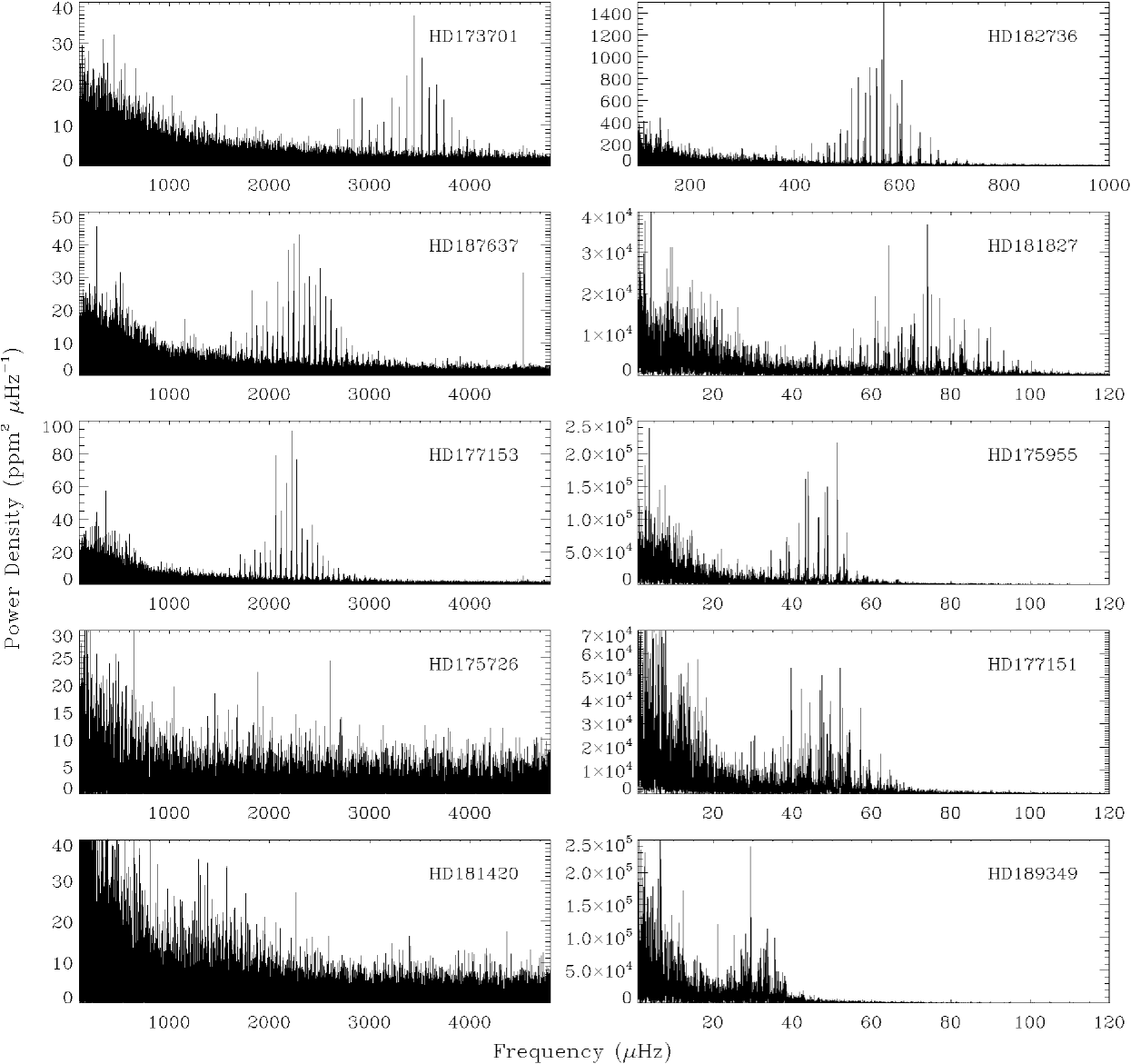
Figure 2.— Power density spectra for all stars in our sample, sorted by the frequency of maximum power ($\nu_{\rm max}$). Note the change in x-axis scale for main-sequence (left column), subgiant (top right column) and red-giant stars (four bottom right panels). Note that the high peak at $\sim$ 4500$\mu$Hz for HD 187637 is a known artefact of Kepler short-cadence data (Gilliland et al., 2010a).

Figure 2 presents the power spectrum for each star, sorted by the frequency of maximum power ($\nu_{\rm max}$). In most cases, a clear power excess due to solar-like oscillations is visible. A summary of the datasets used in our analysis, as well as the derived asteroseismic parameters, is given in Table 3. The analysis of Kepler stars is based on either short-cadence (Gilliland et al., 2010a) or long-cadence (Jenkins et al., 2010) data up to Q10, which were corrected for instrumental trends as described in García et al. (2011). Global asteroseismic parameters were extracted using the automated analysis pipeline by Huber et al. (2009), which has been shown to agree well with other methods (Hekker et al., 2011c; Verner et al., 2011). Due to the length and very high S/N of the Kepler data, the modes are resolved and uncertainties on $\nu_{\rm max}$ and (particularly) $\Delta\nu$ are dominated by the adopted method (e.g., the range over which $\Delta\nu$ is determined) rather than measurement errors. To account for this, we added in quadrature to the formal uncertainties an uncertainty based on the scatter of different methods used by Silva Aguirre et al. (2012) for short-cadence data and by Huber et al. (2011) for long-cadence data. The analysis by Huber et al. (2011) was based on data spanning from Q0-6, which in most cases was sufficient to resolve the modes and reliably estimate $\nu_{\rm max}$ and $\Delta\nu$ (Hekker et al., 2012). In general, the uncertainties on the asteroseismic parameters for most Kepler stars are negligible compared to the uncertainties on other observables. A notable exception is HD 189349, with a relatively large uncertainty of $\sim 4$% in the large frequency separation. Inspection of the power spectrum shows that the modes for this star are very broad, making a determination of $\Delta\nu$ difficult. We speculate that the unusually broad modes may be related to the low metallicity of this object, but a more in-depth analysis is beyond the scope of this paper.

Table 3Asteroseismic observations and measured parameters.

HD	KIC	Data	T (d)	Duty cycle (%)	$\nu_{\rm max}$($\mu$Hz)	$\Delta\nu$($\mu$Hz)
173701	8006161	Kepler SC Q5-10	557	92	3619(98)	149.3(4)
1757261	–	CoRoT SRc01	28	90	1915(200)	97.2(5)
177153	6106415	Kepler SC Q6-8,10	461	70	2233(60)	104.3(3)
181420	–	CoRoT LRc01	156	90	1574(31)	75.1(3)
182736	8751420	Kepler SC Q5,7-10	557	75	568(15)	34.6(1)
187637	6225718	Kepler SC Q6-10	461	91	2352(66)	105.8(3)
175955	10323222	Kepler LC Q0-10	880	91	46.7(1.1)	4.86(3)
177151	10716853	Kepler LC Q1-7,9-10	869	77	48.8(1.1)	4.98(7)
181827	8813946	Kepler LC Q1-10	869	91	73.1(1.2)	6.45(7)
189349	5737655	Kepler LC Q1-10	869	91	29.9(1.1)	4.22(16)

For the two CoRoT stars in our sample, we have re-analyzed publicly available data using the method described in Huber et al. (2009). Our results for HD181420 are in good agreement with the values published by Barban et al. (2009). For HD175726, our analysis did not yield significant evidence for regularly spaced peaks, and yielded only marginal evidence for a power excess at $1900\pm 200\mbox{$\mu$Hz}$. Mosser et al. (2009) have argued that this power excess is compatible with solar-like oscillations and showed evidence for a large variation of $\Delta\nu$ with frequency, which could be responsible for the null-detection in our analysis. We have adopted the published value for $\Delta\nu$ by Mosser et al. (2009) and a value for $\nu_{\rm max}$ corresponding to the maximum of the power excess in the spectrum, with a conservative uncertainty of 10%.

3.2. Interferometry

Interferometric observations were made with the Precision Astronomical Visible Observations (PAVO) beam combiner (Ireland et al., 2008) at the Center for High Angular Resolution Astronomy (CHARA) on Mt. Wilson observatory, California (ten Brummelaar et al., 2005). Operating at a central wavelength of $\lambda=0.7\,\mu$m with baselines up to 330 m, PAVO at CHARA is one of the highest angular-resolution instruments world-wide.

A complete description of the instrument was given by Ireland et al. (2008), and we summarize the basic aspects here. The light from up to three telescopes passes through vacuum tubes and into a series of optics to compensate the path difference. The beams are then collimated and passed through a non-redundant mask which acts as a bandpass filter, and spatially modulated interference fringes are formed behind the mask. The interference pattern is then passed through a lenslet array and a prism, producing fringes in 16 segments on the CCD detector, each being spectrally dispersed in several independent wavelength channels. Major advantages of the PAVO design are high sensitivity (with a limiting magnitude of $R\sim 8$ mag in typical seeing conditions), increased information through spectral dispersion, and high spatial resolution through operating at visible wavelengths. First PAVO science results have been presented by Bazot et al. (2011), Derekas et al. (2011) and Huber et al. (2012). For our analysis, we have used PAVO observations in two-telescope mode, with baselines ranging from $\sim 110-330$ m.

Table 4Calibrators used for interferometric observations.

HD	Sp.T.	$V-K$	$E(B-V)$	$\theta_{V-K}$	ID
171654	A0V	-0.067	0.036	0.141	c
174177	A0V	0.249	0.020	0.191	gh
176131	A2V	0.345	0.012	0.155	ac
176626	A2V	0.084	0.026	0.146	ac
177959	A3V	0.451	0.029	0.152	b
178190	A2V	0.381	0.027	0.157	bd
179095	A0V	-0.069	0.022	0.129	gh
179124	B9V	0.280	0.095	0.146	d
179483	A2V	0.316	0.028	0.144	e
179733	A0V	0.211	0.038	0.117	ac
180138	A0V	0.075	0.045	0.128	c
180501	A0V	0.147	0.027	0.117	gh
180681	A0V	0.112	0.031	0.111	acei
183142	B8V	-0.462	0.060	0.093	ei
184147	A0V	0.007	0.019	0.121	egi
184787	A0V	0.034	0.017	0.154	cf
188252	B2III	-0.461	0.047	0.155	ce
188461	B3V	-0.461	0.109	0.095	efj
189845	A0V	0.136	0.053	0.127	fj
190025	B5V	-0.230	0.157	0.084	j
190112	A0V	0.067	0.027	0.113	f

List of dropped calibrators: HD179395, HD181939, HD182487, HD184875, HD189253; “ID” refers to the ID of the target star for which the calibrator has been used (see column 3 of Table 5).

Table 5Interferometric observations and measured parameters.

HD	KIC	ID	Scans/Nights	Baselines	$\mu_{R}$	$\theta_{\rm UD}$	$\theta_{\rm LD}$	$\theta_{(V-K)}$	$\theta_{\rm IRFM}$
173701	8006161	a	9/4	S2E2,S1W1,S1E2,S1E1	$0.59(4)$	$0.314(4)$	$0.332(6)$	$0.333(5)$	$0.32(1)$
175726	–	b	3/2	S1W2,S1E1	$0.51(5)$	$0.331(5)$	$0.346(7)$	$0.356(5)$	$0.35(2)$
177153	6106415	c	7/3	S2E2,S1W1,S1E2	$0.51(5)$	$0.276(6)$	$0.289(6)$	$0.285(4)$	$0.28(1)$
181420	–	d	5/2	S1W2,S1E1	$0.48(5)$	$0.32(1)$	$0.34(1)$	$0.312(5)$	$0.31(1)$
182736	8751420	e	5/4	S2W2,S2E2,S1W1	$0.59(4)$	$0.412(3)$	$0.436(5)$	$0.429(6)$	$0.44(2)$
187637	6225718	f	6/3	S2E2,S1E2,S1E1	$0.49(5)$	$0.222(5)$	$0.231(6)$	$0.222(3)$	$0.22(1)$
175955	10323222	g	4/2	W1W2,S2W2	$0.67(2)$	$0.634(9)$	$0.68(1)$	$0.70(1)$	$0.66(3)$
177151	10716853	h	4/2	W1W2,S2W2	$0.64(3)$	$0.541(8)$	$0.57(1)$	$0.57(1)$	$0.53(2)$
181827	8813946	i	3/2	S2W2,S1W1	$0.64(3)$	$0.443(3)$	$0.473(5)$	$0.516(9)$	$0.49(2)$
189349	5737655	j	4/3	S2W2,S1W2	$0.58(4)$	$0.399(4)$	$0.420(6)$	$0.444(9)$	$0.44(2)$

“ID” can be used in Table 4 to identify which stars have been used to calibrate this target. All angular diameters are given in units of milli-arcseconds. Baselines are sorted from shortest to longest length for a given target.

Interferometric observations require careful calibration of the observed visibilities. Ideally, this is achieved by observing bright, unresolved point sources as closely as possible to the target object in time and distance. For PAVO observations of targets as small as in our case, this means calibrating with late B to early A stars since at the PAVO magnitude limit these stars are distant enough to have significantly smaller diameters (0.1–0.15 mas) than our target stars. Table 4 lists all calibrators that were used in our analysis. Expected sizes are calculated using the $V-K$ relation by Kervella et al. (2004) for dwarf and subgiant stars. $V$ band magnitudes have been taken from the Tycho catalog and were converted into the Johnson system using the calibration by Bessell (2000). $K$ magnitudes were adopted from 2MASS (Skrutskie et al., 2006). Interstellar reddening for each calibrator was estimated using the extinction model by Drimmel et al. (2003).

Although we have checked each calibrator in the literature for possible multiplicity, rotation and variability prior to observations, our data show that roughly 1/4 of all observed calibrators are more resolved than expected, and therefore potentially unsuitable for calibration. These calibrators are listed at the bottom of Table 4. Possible reasons for this include previously undetected binary systems and rapid rotation causing deviations from spherical symmetry.

Figure 3 presents the calibrated squared-visibility measurements as a function of spatial frequency for all targets in our sample, with a summary of observations given in Table 5. We have collected at least three independent scans for each target over at least two different nights, and the visibilities of each target were calibrated with at least two different calibrators (see also Table 4). Note that each scan typically produces a measurement of visibility in 20 independent wavelength channels, resulting in a total of $\sim$1000 visibility measurements in our campaign.

For each target we fitted the following limb-darkened disc model to the observations (Hanbury Brown et al., 1974):

$$V=\left(\frac{1-\mu_{\lambda}}{2}+\frac{\mu_{\lambda}}{3}\right)^{-1}\\ \times\left[(1-\mu_{\lambda})\frac{J_{1}(x)}{x}+\mu_{\lambda}(\pi/2)^{1/2}\frac{J_{3/2}(x)}{x^{3/2}}\right]\>,$$ (1)

with

$$x=\pi B\theta_{\rm LD}\lambda^{-1}\>.$$ (2)

Here, $V$ is the visibility, $\mu_{\lambda}$ is the linear limb-darkening coefficient, $J_{n}(x)$ is the $n$-th order Bessel function, $B$ is the projected baseline, $\theta_{\rm LD}$ is the angular diameter after correction for limb-darkening, and $\lambda$ is the wavelength at which the observation was made. Linear limb-darkening coefficients in the $R$ band for our targets were estimated by interpolating the model grid of Claret & Bloemen (2011) to the spectroscopic estimates of $T_{\rm eff}$, $\log g$ and [Fe/H] (Table 1) for a microturbulent velocity of 2 km s^-1. Uncertainties on the limb-darkening coefficients were estimated from the difference in the methods presented by Claret & Bloemen (2011). The choice of the limb-darkening model has little effect on the final fitted angular diameters. Detailed 3-D hydrodynamical models by Bigot et al. (2006), Chiavassa et al. (2010) and Chiavassa et al. (2012) for dwarfs and giants have shown that the differences to simple linear limb darkening models are 1% or less in angular diameter for stars with near solar-metallicity. For a moderately resolved star with $V^{2}\sim 0.5$, a 1% change in angular diameter would arise from a change of less than 1% in $V^{2}$, which is less than our typical measurement uncertainties.

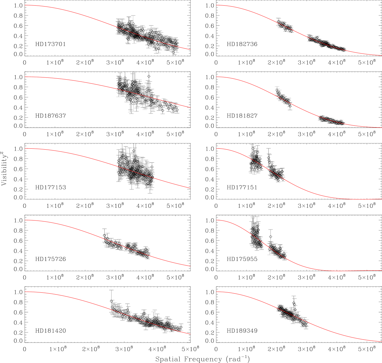
Figure 3.— Squared visibility versus spatial frequency for all stars in our sample. Red solid lines show the fitted limb-darkened disc model. The order of panels is the same as in Figure 2. Note that the error bars for each star have been scaled so that the reduced $\chi^{2}$ equals unity.

The procedure used to fit the model and estimate the uncertainty in the derived angular diameters was described by Derekas et al. (2011). In summary, Monte-Carlo simulations were performed which took into account uncertainties in the adopted wavelength calibration (0.5%), calibrator sizes (5%), limb-darkening coefficients (see Table 5), as well as potential correlations across wavelength channels. The resulting fitted angular diameters of each target, corrected for limb-darkening, are given in Table 5. We also give the uniform-disc diameters in Table 5, which were derived by setting $\mu_{\lambda}=0$ in Equation (1).

A few comments on our derived diameters are necessary. Firstly, one calibrator in our sample (HD 179124), which is the main calibrator for HD 181420, was recently found to be a rapidly rotating B star with $v\sin i=290$ km/s (Lefever et al., 2010). This introduces an extra uncertainty on the estimated calibrator diameter. We have accounted for this by assuming a 20% uncertainty in the calibrator diameter, which roughly corresponds to the maximum change in the average diameter expected for rapid rotators (Domiciano de Souza et al., 2002). Secondly, a few of our target stars (e.g. HD 187637) are only about 50% bigger in angular size than their calibrators. This means that the uncertainties on the derived diameters will be strongly influenced by the assumed uncertainties of the calibrator diameters, which in our case are 5%. While such an uncertainty is reasonable compared to the scatter in the photometric calibrations (see, e.g., Kervella et al., 2004), the diameter measurement itself will only be scientifically useful if the uncertainty in the measured diameter is smaller than the precision of indirect techniques. Further data at longer baselines with smaller calibrators will be needed to reduce the uncertainties for these targets.

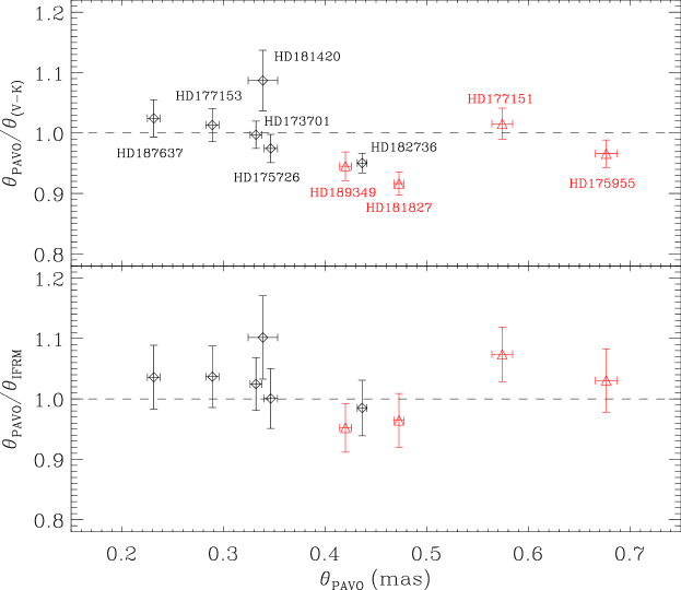
Figure 4.— Fractional differences between angular diameters measured with PAVO to diameters determined using the $(V-K)$ surface-brightness relation by Kervella et al. (2004) (upper panel) and using the infrared flux method with asteroseismic constraints, as described in Silva Aguirre et al. (2012) (lower panel). Black diamonds show main-sequence and subgiants stars, and red triangles show giant stars. HD numbers of each target are labelled in the upper panel.

Indirect techniques to estimate angular diameters include surface brightness relations (see, e.g., van Belle, 1999; Kervella et al., 2004) and the infrared flux method (IRFM, see, e.g., Ramírez & Meléndez, 2005; Casagrande et al., 2010). Figure 4 compares our measured angular diameters with predictions using the $(V-K)$ surface-brightness relation for dwarfs and subgiants by Kervella et al. (2004) and the IRFM method coupled with asteroseismic constraints, as described in Silva Aguirre et al. (2012). For the $(V-K)$ relation we have adopted a 1% diameter uncertainty for all stars (Kervella et al., 2004). We find good agreement for all stars for both methods, with a residual mean of $-2\pm 2$% and $+2\pm 2$% for $(V-K)$ and IRFM, respectively, both with a scatter of 5%. Our results therefore seem to confirm that the relation by Kervella et al. (2004) is also valid for red giants, as suggested by Piau et al. (2011), and that combining the IRFM method with asteroseismic constraints, as done by Silva Aguirre et al. (2012), yields accurate diameters for both evolved and unevolved stars.

These tests of indirect methods are encouraging. We emphasize that interferometry remains an important tool to validate these methods for a wider range of evolutionary states, chemical compositions, and distances. The $(V-K)$ relation, for example, is based on an empirical relation calibrated using nearby stars that does not take into account potential spread due to different chemical compositions, and is only valid for de-reddened magnitudes. An illustration of the importance of using interferometry is HD 181827, which shows a significantly smaller measured diameter than predicted from $(V-K)$. This smaller diameter is also in agreement with asteroseismic results, which suggest a smaller radius (see Section 4.1).

3.3. Bolometric Fluxes

To estimate bolometric fluxes for our target sample, we first extracted synthetic fluxes from the MARCS database of stellar model atmospheres (Gustafsson et al., 2008). We used models with standard chemical composition, with the microturbulence parameter set to 1 km s^-1 for plane-parallel models (unevolved stars) and 2 km s^-1 for spherical models with a mass of 1$M_{\sun}$ for red giants. We then multiplied the synthetic stellar fluxes by the filter responses for the Johnson-Glass-Cousins $UBVRIJHKL$, Tycho $B_{\rm T}V_{\rm T}$ and 2MASS $JHK_{\rm s}$ systems and integrated the resulting fluxes to calculate synthetic magnitudes for each MARCS model. Filter responses and zeropoints were taken from Bessell & Murphy (2012) ($UBVRI$, $B_{\rm T}V_{\rm T}$), Cohen et al. (2003) (2MASS), and Bessell et al. (1998) ($JHKL$). We note that synthetic photometry calculated using MARCS models has previously been validated using observed colors in stellar clusters (Brasseur et al., 2010; VandenBerg et al., 2010). To check the influence of the chosen mass for the spherical models, we have repeated the above calculations for typical red giant models with $T_{\rm eff}=5000$ K and $\log g=2-3$. The fractional differences in the integrated flux for each filter for masses ranging from $0.5-5\mbox{$M_{\sun}$}$ was found to be less than 0.5% in all bands, and are therefore negligible for our analysis.

The amount of photometry in the literature for our sample is unfortunately small. The targets are generally too faint to have reliable magnitudes in the Johnson-Glass-Cousins system, and they are too bright to have a full set of SDSS photometry in the KIC. To ensure consistency of our bolometric fluxes we only used photometry that is available for all stars in our sample, namely Tycho2 $B_{T}V_{T}$ and 2MASS $JHK_{\rm s}$ magnitudes. The adopted photometry and uncertainties are listed in Table 6.

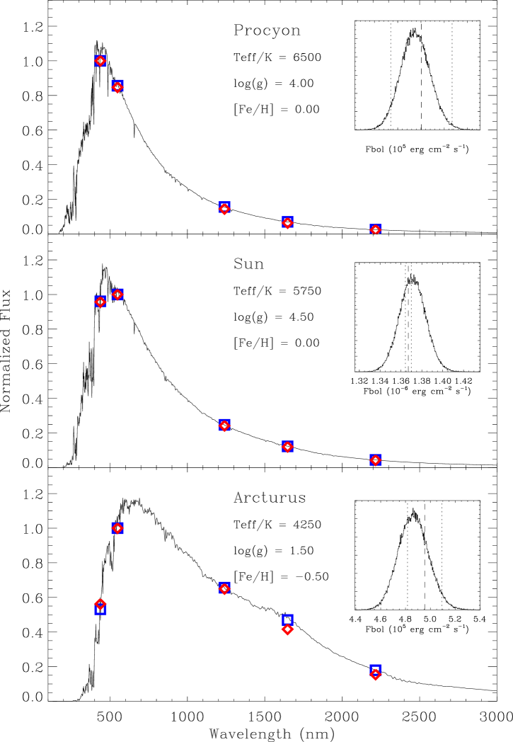
Figure 5.— Spectral energy distibutions of Procyon, the Sun and Arcturus to test our method to determine bolometric fluxes. Black lines are MARCS models with parameters as given in each panel, smoothed with a constant spectral resolution $\lambda/\Delta\lambda\sim 200$ (corresponding to a width of $\sim$2.5 nm in the V-band). Observed and synthetic $BVJHK$ photometry is shown as red diamonds and blue squares, respectively. All fluxes have been normalized to 1 in the band with highest flux for a given star. The inset shows the result of Monte-Carlo simulations to estimate the uncertainty in the bolometric flux as described in the text. Dashed and dotted lines show the literature values and 1-$\sigma$ uncertainties.

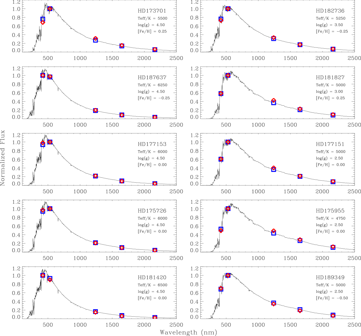
Figure 6.— Spectral energy distributions for all stars in our sample. Black lines are the MARCS models with parameters as given in each panel, smoothed with a constant spectral resolution $\lambda/\Delta\lambda\sim 200$ (corresponding to a width of $\sim$2.5 nm in the V-band). Red diamonds and blue squares show the observed and model fluxes in the $B_{T}V_{T}JHK$ bands, respectively. All fluxes have been normalized to 1 in the band with highest flux for a given star. The order of panels is the same as in Figure 2.

To calculate bolometric fluxes, we largely followed the approach described in Alonso et al. (1995). For each target star, we first found the six models bracketing the spectroscopic determinations $T_{\rm eff}$, $\log g$ and [Fe/H], as given in Table 1. We then transformed the synthetic $B_{T}V_{T}JHK_{\rm s}$ magnitudes of each model into fluxes, and numerically integrated these fluxes using the pivot wavelength for each filter response, calculated as described by Bessell & Murphy (2012) (note that this choice of a reference wavelength is independent of the spectral type considered). The numerical integration yielded an estimate $f_{\rm int}$, which we then compared to the true bolometric flux, $f_{\rm bol}=\sigma T_{\rm eff}^{4}$, where $\sigma$ is the Stefan-Boltzmann constant. This yielded a correction factor $c=f_{\rm int}/f_{\rm bol}$ for each of the six models, which gave the percentage of flux included when integrating the photometry over discrete wavelengths. The final bolometric flux was then calculated by integrating the observed fluxes the same way as the model fluxes, and dividing the resulting estimate by the correction factor $c$ found by interpolating the six corrections factors to the spectroscopic estimates of $T_{\rm eff}$, $\log g$ and [Fe/H]. Note that this interpolation was necessary because the step size of the MARCS grid is typically larger than the uncertainties of the spectroscopic parameters. Uncertainties in the derived bolometric fluxes were found by perturbing the input photometry and the spectroscopic parameters according to their estimated uncertainties (see Tables 1 and 6), repeating the procedure 5000 times, and taking the standard deviation of the resulting distribution.

Table 6Broadband photometry, estimated reddening and bolometric fluxes for all target stars.

HD	KIC	$B_{\rm T}$	$V_{\rm T}$	$J$	$H$	$K$	$E(B-V)$	Fbol ($10^{-8}$ erg s-1 cm-2)
								MARCS	ATLAS+$\theta$	ATLAS+$V_{\rm T}$
173701	8006161	$8.606(16)$	$7.610(11)$	$6.088(21)$	$5.751(16)$	$5.670(21)$	0.000(5)	$2.89(5)$	$2.93(4)$	$2.86(3)$
175726	–	$7.401(15)$	$6.780(10)$	$5.703(24)$	$5.418(34)$	$5.346(20)$	0.000(5)	$5.4(1)$	$5.40(7)$	$5.41(6)$
177153	6106415	$7.872(15)$	$7.275(11)$	$6.145(20)$	$5.923(26)$	$5.829(23)$	0.000(5)	$3.39(7)$	–	–
181420	–	$7.059(15)$	$6.604(10)$	$5.748(21)$	$5.560(33)$	$5.513(26)$	0.000(5)	$6.0(2)$	$6.2(1)$	$5.99(7)$
182736	8751420	$8.021(16)$	$7.103(10)$	$5.515(24)$	$5.135(27)$	$5.028(16)$	0.000(5)	$4.77(8)$	$4.74(5)$	$4.67(5)$
187637	6225718	$8.118(15)$	$7.580(11)$	$6.544(21)$	$6.346(29)$	$6.283(18)$	0.000(5)	$2.55(5)$	–	–
175955	10323222	$8.513(16)$	$7.146(10)$	$4.999(24)$	$4.442(31)$	$4.318(17)$	0.09(2)	$7.2(3)$	–	–
177151	10716853	$8.281(16)$	$7.144(10)$	$5.264(18)$	$4.820(33)$	$4.686(20)$	0.04(2)	$5.6(3)$	–	–
181827	8813946	$8.476(15)$	$7.300(10)$	$5.453(35)$	$4.997(15)$	$4.872(21)$	0.04(2)	$4.8(2)$	–	–
189349	5737655	$8.411(16)$	$7.411(10)$	$5.638(24)$	$5.181(21)$	$5.124(29)$	0.07(2)	$4.6(2)$	–	–

To test this approach, we have used the same method for three bright stars that span a similar range of evolutionary stages as our sample and for which bolometric fluxes have been well determined: Procyon, the Sun, and Arcturus. Since Tycho and 2MASS photometry is not available for such bright stars, we have used $BVJHK$ photometry to mimic the available information for our target sample. Photometry has been taken from the General Catalog of Photometric Data (GCDP, Mermilliod et al., 1997) for Procyon and Arcturus, and from Colina et al. (1996) for the Sun. Figure 5 shows the spectral energy distributions (SEDs) of all three stars, comparing the MARCS model that best matches the physical parameters of each star (black line) to the observed and synthetic fluxes in the $BVJHK$ bands (red and blue squares, respectively). Note that the MARCS models have been smoothed to a spectral resolution of $\lambda/\Delta\lambda\sim 200$ for better visibility. The insets show the distributions of the Monte-Carlo simulations described above compared to the literature values of the bolometric flux (dashed line) and their 1-$\sigma$ uncertainties (dotted lines). Literature bolometric fluxes have been taken from Ramírez & Allende Prieto (2011) for Arcturus, Aufdenberg et al. (2005) and Fuhrmann et al. (1997) for Procyon, and we have adopted an effective temperature of $5777\pm 3$ K for the Sun. In all three cases, the bolometric flux using our method is recovered within 1-$\sigma$, with a maximum deviation of $\sim$0.5 $\sigma$ for Arcturus.

Figure 6 shows the SEDs of all target stars with the appropriate models for each star, and Table 6 lists our bolometric fluxes based on the procedure described above. We note that for the red giants in our sample, interstellar reddening cannot be neglected. To estimate reddening using the SED, we adopted the reddening law by O’Donnell (1994) (see also Cardelli et al., 1989) and iterated over $E(B-V)$ to find the observed colors that best fit the colors of the six models bracketing the spectroscopic parameters in Table 1. We then again interpolated to the spectroscopic $T_{\rm eff}$, $\log g$ and [Fe/H] values, analogously to the correction factor described above. The derived reddening estimates for the giants are listed in Table 6.

To further test these results, we have used an independent method to determine bolometric fluxes for four stars by combining publicly available flux-calibrated ELODIE spectra (Prugniel et al., 2007), broadband photometry and ATLAS9 models (Castelli & Kurucz, 2003, 2004). We started by calculating a grid of ATLAS9 models in the 3-$\sigma$ error box of the spectroscopically determined $T_{\rm eff}$, $\log g$ and [Fe/H] (see Table 1). Each model spectrum was then multiplied by the $B_{\rm T}V_{\rm T}JHK_{\rm s}$ filter passbands and integrated over all wavelengths to compute a synthetic flux in each band. Model fluxes were then calibrated into fluxes received on Earth using either the measured angular diameter or the Tycho $V_{T}$ magnitude. To find the model that best fits the photometric data we then compared the grid of model fluxes with the observed fluxes, calculated using the same zeropoints as in the procedure described above. Finally, the bolometric flux of each star was determined by integrating the ELODIE spectrum between 390 and 680 nm together with the synthetic ATLAS9 model (covering the wavelength ranges $<390$ nm and $>680$ nm) that best fits the observed photometry.

To estimate uncertainties the above procedure was repeated 100 times, drawing random values for the observed photometry given in Table 6, and adding the standard deviation of the resulting distribution in quadrature to the uncertainty of the total flux of the ELODIE spectra. The final values for the two different calibration methods are given in Table 6. The derived bolometric fluxes agree well with the estimates from MARCS models, reassuring us that the model dependency and adopted method have little influence compared to the estimated uncertainties. We note that we have also compared our bolometric fluxes with estimates derived from the infrared flux method, as described in Silva Aguirre et al. (2012). Again, we have found good agreement with our estimates within the quoted uncertainties.

4. Fundamental Stellar Properties

4.1. Asteroseismic Scaling Relations

The large frequency separation of oscillation modes with the same spherical degree and consecutive radial order is closely related to the mean density of star (Ulrich, 1986):

$$\Delta\nu\propto M^{1/2}R^{-3/2}\>.$$ (3)

Additionally, Brown et al. (1991) argued that the frequency of maximum power ($\nu_{\rm max}$) for solar-like stars should scale with the acoustic cut-off frequency, which was used by Kjeldsen & Bedding (1995) to formulate a second scaling relation:

$$\nu_{\rm max}\propto MR^{-2}T_{\rm eff}^{-1/2}\>.$$ (4)

Provided the effective temperature of a star is known, Equations (3) and (4) allow an estimate of the stellar mass and radius. This can be done by either combining the two equations (the so-called direct method, see Kallinger et al., 2010c) or by comparing the observed values of $\Delta\nu$ and $\nu_{\rm max}$ with values calculated from a grid of evolutionary models (the so-called grid-based method, see Stello et al., 2009b; Basu et al., 2010; Gai et al., 2011).

Our interferometric observations, presented in the Section 3.2, allow us to test Equations (3) and (4). Using the Hipparcos parallaxes in combination with the angular diameters, we have calculated linear radii for our sample of stars, which are listed in Table 7. These are compared to asteroseismic radii calculated using Equations (3) and (4) (using $T_{\rm eff}$ values taken from Table 1) in Figure 7. Note the influence of $T_{\rm eff}$ on Equation (4) is small: for solar $T_{\rm eff}$ a variation of 100 K causes only a 0.9% change in $\nu_{\rm max}$, which is significantly smaller than our typical uncertainties (see Table 3).

The comparison in Figure 7 is very encouraging, showing an agreement between the two methods within 3-$\sigma$ in all cases. The overall scatter about the residuals is $\sim$13%, and we do not observe any systematic trend as a function of size (and therefore stellar properties). We note that two of the stars in our sample (HD 173701 and HD 177153) have also been analyzed by Mathur et al. (2012), who used both a grid-based approach as well as detailed modelling of individual oscillation frequencies to derive stellar radii and masses. In both cases, the radii from different models presented in Mathur et al. (2012) slightly improve the difference to the interferometrically measured radius, with minimum differences of +0.4 $\sigma$ and +0.8 $\sigma$ compared to differences of -0.6 $\sigma$ and -1.0 $\sigma$ from the direct method, respectively.

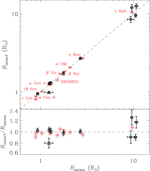
Figure 7.— Comparison of stellar radii measured using interferometry and calculated using asteroseismic scaling relations. Black diamonds show our Kepler and CoRoT sample, and red asterisks show several bright stars as indicated in the plot for comparison. The dashed line marks the 1:1 relation.

For comparison, Figure 7 also shows examples of bright stars for which well constrained asteroseismic and interferometric parameters are available. We have adopted values for $\Delta\nu$ and $\nu_{\rm max}$ from Stello et al. (2009a) and references therein, with uncertainties fixed to typical values of 1% in $\Delta\nu$ and 3% in $\nu_{\rm max}$. Asteroseismic observations have been obtained from the MOST space telescope for $\epsilon$ Oph (Barban et al., 2007; Kallinger et al., 2008), the CoRoT space-telescope for HD 49933 (Appourchaux et al., 2008), and from ground-based Doppler observations for the remaining sample (Carrier & Bourban, 2003; Kjeldsen et al., 2003; Bedding et al., 2004; Carrier et al., 2005a, b; Kjeldsen et al., 2005; Bedding et al., 2007; Arentoft et al., 2008; Teixeira et al., 2009; Bazot et al., 2011). Angular diameters and effective temperatures were taken from Mazumdar et al. (2009) and De Ridder et al. (2006) for $\epsilon$ Oph, Bazot et al. (2011) for 18 Sco, Bigot et al. (2011) for HD 49933 and from Bruntt et al. (2010) and references therein for the remaining sample. Parallaxes were adopted from van Leeuwen (2007), except for $\alpha$ Cen A and B for which we have adopted the value by Söderhjelm (1999). Figure 7 again shows agreement within 3-$\sigma$ in all cases. Excluding HD 175726 from our sample due to large uncertainties in the asteroseismic observations, the residual scatter between asteroseismic and interferometric radii is 4% for dwarfs and 16% for giants, with mean deviations of $-1\pm 1$ % and $+6\pm 4$ %, respectively. This is consistent with our observational uncertainties and hence empirically confirms that, at least for main-sequence stars, asteroseismic radii from scaling relations are accurate to $\lesssim 4\%$. Note that Miglio (2012) has previously found a similar good agreement for a sample of nearby stars, with a residual scatter of 6%.

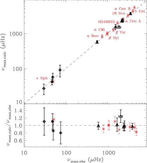
Figure 8.— Comparison of $\nu_{\rm max}$ measured from asteroseismology and calculated using independent measurements of R, M and $T_{\rm eff}$. Black diamonds show the Kepler and CoRoT sample, and red asterisks show several bright stars as indicated in the plot for comparison. The dashed line marks the 1:1 relation.

It is well known that the scaling relation for $\Delta\nu$ is on more solid ground than the scaling relation for $\nu_{\rm max}$, which only recently has been studied in more detail observationally (see, e.g., Stello et al., 2009a; Mosser et al., 2010; White et al., 2011) and theoretically (Belkacem et al., 2011). To test Equation (4), we can combine Equation (3) with the interferometrically measured radii to calculate stellar masses, and combine these with $T_{\rm eff}$ to calculate $\nu_{\rm max}$. We compare these with the measured values in Figure 8. We again observe good agreement within the error bars, with no systematic deviation as a function of evolutionary status. Figure 8 also displays a comparison with measured values for a sample of bright stars, again showing good agreement with our results for the Kepler and CoRoT sample. We note that Bedding (2011) has shown a similar comparison for bright stars, and noted a potential breakdown of the $\nu_{\rm max}$ relation for low-mass stars with $\mbox{$\nu_{\rm max}$}\gtrsim 4500\mbox{$\mu$Hz}$. Since none of the stars in our sample have $\mbox{$\nu_{\rm max}$}>4000\mbox{$\mu$Hz}$, we are unable to test this claim in our study.

The large error bars for some stars in Figures 7 and 8 may cast some doubt about the usefulness of interferometry to test scaling relations. Indeed, for the red giants in our sample the uncertainty in the interferometric radius is completely dominated by the uncertainty in the parallax. For these stars the PAVO data will be most valuable to measure the effective temperature by combining the angular diameter with an estimate of the bolometric flux, which can then be compared to indirect $T_{\rm eff}$ estimates from broadband photometry and spectroscopy (see next section). For most unevolved stars in the Kepler/CoRoT sample, our current uncertainties in the angular diameters are comparable to the parallax uncertainties. The bright star comparison sample, on the other hand, is dominated by the uncertainties in the asteroseismic observables, which are much more difficult to constrain from the ground or using smaller space telescopes. The fact that the asteroseismic uncertainties are almost negligible for the Kepler/CoRoT sample explains the somewhat counter-intuitive observation that the error bars in Figures 7 and 8 are similar for some stars of the Kepler sample and for stars which are up to 8 magnitudes brighter. This comparison underlines the importance of obtaining precise asteroseismic constraints on bright stars for which constraints are available from independent observational techniques.

4.2. Spectroscopic and Photometric Temperatures

The measurement of the angular diameter $\theta_{\rm LD}$ of a star combined with an estimate of its bolometric flux $f_{\rm bol}$ allows a direct measurement of the effective temperature:

$$T_{\rm eff}=\left(\frac{4f_{\rm Bol}}{\sigma\theta_{\rm LD}^{2}}\right)^{1/4}\>,$$ (5)

where $\sigma$ is the Stefan-Boltzmann constant. We have used our measured angular diameters presented in Section 3.2 together with the bolometric flux estimates presented in Section 3.3 to calculate effective temperatures for our sample, which are listed in Table 7.

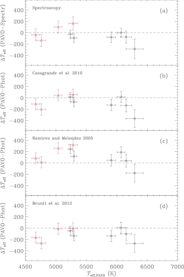
Figure 9.— Comparison of effective temperatures derived in this study with spectroscopic estimates (panel a) and several photometric calibrations based on $V-K_{\rm s}$ (panels b–d). Black diamonds are main-sequence stars, while red triangles show red giants. Note that the relations by Casagrande et al. (2010) and Bruntt et al. (2012) are calibrated for main-sequence stars.

The model dependency of effective temperatures calculated using Equation (5) is small, and hence such estimates are important for calibrating indirect photometric estimates such as the infrared flux method (see, e.g., Casagrande et al., 2010), as well as spectroscopic determinations for which usually strong degeneracies between $T_{\rm eff}$, $\log g$ and [Fe/H] exist (see, e.g., Torres et al., 2012). Figure 9 compares the measured effective temperatures in our sample to estimates from high-resolution spectroscopy (mostly using the VWA package by Bruntt et al. (2010), see Table 1) as well as photometric calibrations taken from Casagrande et al. (2010), Ramírez & Meléndez (2005) and Bruntt et al. (2012). We have chosen $V-K_{\rm s}$ to calculate photometric temperatures since this index usually gives the lowest residuals as a temperature indicator for cool stars (see, e.g., Casagrande et al., 2010). The comparison in Figure 9a shows good agreement of our temperatures with spectroscopy, with a residual mean of $-48\pm 39$ K with a scatter of 124 K for all stars, and $-22\pm 33$ K with a scatter of 97 K when excluding the F-star HD 181420 for which the angular diameter is not well determined. We note that this agreement is only slightly worse (with an increased scatter by about 10 K) if we use the $T_{\rm eff}$ values by Bruntt et al. (2012) and Thygesen et al. (2012) for which no asteroseismic constraints on $\log g$ were used. Bruntt et al. (2010) noted that a slight bias for spectroscopic temperatures to be hotter than interferometric estimates by $\sim 40\,$K for a sample of nearby stars, which is somewhat confirmed by our results, although the scatter is significantly larger. Our result confirms that a combination of spectroscopy and asteroseismology can be applied for the accurate characterization of temperatures, radii and masses of much fainter stars, e.g. exoplanet host stars observed by the Kepler mission.

The photometric estimates shown in Figure 9b, 9c and 9d show slight systematic deviations. The calibration by Casagrande et al. (2010) shows the best agreement, with only the coolest red giants being slightly hotter than implied by our results. The calibration by Ramírez & Meléndez (2005) is the only one that directly provides color-temperature relations calibrated for giants. As already noted by Casagrande et al. (2010), the temperatures by Ramírez & Meléndez (2005) seem to be systematically cooler than expected, and this is confirmed by our results. Finally, the calibration given by Bruntt et al. (2012) overestimates temperatures at the cool end, which is again not surprising since their calibration was based on main-sequence stars only, and did not include corrections for lower surface gravities and different metallicities. Overall, we conclude that photometric estimates reproduce the measured temperatures from interferometry well within the uncertainties, except for the giants where reddening is significant. We note that HD 173701 is the only star with sufficient Sloan photometry to be included in the calibration by Pinsonneault et al. (2012). The SDSS temperature, corrected for metallicity as described in Pinsonneault et al. (2012), is $5364\pm 100$ K, in good agreement to the determined values here. Finally, we note that the effective temperatures presented in this section do not influence the comparisons of the asteroseismic masses and radii calculated in the previous section (which were calculated using spectroscopic $T_{\rm eff}$), since the dependence of Equation (4) on $T_{\rm eff}$ is only small.

Table 7Fundamental properties of all Kepler and CoRoT stars in this study.

HD	KIC	$T_{\rm eff}$ (K)	[Fe/H]	$R/\mbox{$R_{\sun}$}$	$M/\mbox{$M_{\sun}$}$	$R/$$R_{\sun}$	$M$/$M_{\sun}$	$T_{\rm eff}$ (K)
		Spectroscopy		$\nu_{\rm max}$+$\Delta\nu$+$T_{\rm eff,sp}$		$\pi+\Theta_{\rm LD}$	$\pi+\Theta_{\rm LD}+\mbox{$\Delta\nu$}$	$\Theta_{\rm LD}+f_{\rm bol}$
173701	8006161	5390(60)	$+0.34(6)$	0.926(26)	0.969(82)	0.952(21)	1.054(69)	5295(51)
175726	–	6070(45)	$-0.07(3)$	–	–	0.987(23)	–	6069(65)
177153	6106415	5990(60)	$-0.09(6)$	1.235(35)	1.123(94)	1.289(37)	1.27(11)	5908(72)
181420	–	6580(105)	$+0.00(6)$	1.758(41)	1.68(12)	1.730(84)	1.60(23)	6292(141)
182736	8751420	5264(60)	$-0.15(6)$	2.674(74)	1.26(10)	2.703(71)	1.30(10)	5236(37)
187637	6225718	6230(60)	$-0.17(6)$	1.288(38)	1.31(11)	1.306(47)	1.37(15)	6153(89)
175955	10323222	4706(80)	$+0.06(15)$	10.53(30)	1.51(13)	9.54(50)	1.13(18)	4668(66)
177151	10716853	4898(80)	$-0.10(15)$	10.72(40)	1.67(19)	12.5(1.0)	2.68(64)	4761(70)
181827	8813946	4940(80)	$+0.14(15)$	9.58(28)	2.01(18)	12.0(1.2)	4.0(1.2)	5039(66)
189349	5737655	5118(90)	$-0.56(16)$	9.34(78)	0.79(21)	8.48(76)	0.60(17)	5282(72)

4.3. Stellar Models

Detailed modelling will be deferred to a future paper, but we present some first basic comparisons for the most interesting cases here. We use the publicly available BaSTI stellar evolutionary tracks (Pietrinferni et al., 2004) with solar-scaled distribution of heavy elements (Grevesse & Noels, 1993) and a standard mass loss parameter of $\eta=0.4$ (see, e.g. Fusi-Pecci & Renzini, 1976). The models do not include effects of diffusion or gravitational settling, and are calibrated to match the observed properties of the Sun with a mixing length parameter $\alpha_{\rm MLT}=1.913$ and an initial chemical composition of $(Y,Z)=(0.2734,0.0198)$. No convective-core overshooting was included in the models presented here. Note that in the following we compare models to radii, masses and temperatures derived using our direct measurement of the angular diameter (see columns 7, 8 and 9 in Table 7) and the spectroscopic metallicities.

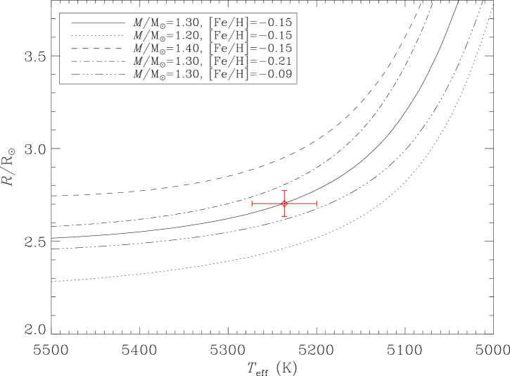
Figure 10.— Radius versus effective temperature with the position of the subgiant HD 182736 shown as a red diamond. The solid line shows the BaSTI evolutionary model matching the metallicity from high-resolution spectroscopy and the mass determined in this study. Dashed-dotted and dashed-triple-dotted lines show the effect of varying the metallicity by 1 $\sigma$, while dotted and dashed lines show the same effect for varying the mass by 1 $\sigma$. The determined mass and metallicity for HD 182736 are $M=1.3\pm 0.1\mbox{$M_{\sun}$}$ and $\rm{[Fe/H]}=-0.15\pm 0.06$.

4.3.1 HD 182736

The star with the best constrained fundamental properties in our sample is the subgiant HD 182736, with relative uncertainties in temperature, radius and mass of 0.7%, 2.6% and 7.7%, respectively. The fact that the best observational result is achieved for the only subgiant in our sample is not surprising: while the more distant red giants generally have well constrained diameters due to their larger size, they suffer from a large uncertainty in the parallaxes and effective temperatures due to their larger distance and significant reddening. On the other hand, main-sequence stars are generally too small to achieve a good precision on their measured diameters. Subgiants land in the ”sweet spot” between these regimes, with angular sizes big enough for a precise measurement with PAVO and distances close enough to have a well constrained Hipparcos parallax and negligible reddening.

Figure 10 shows a diagram of stellar radius versus effective temperature with the position of HD 182736 according to the properties listed in Table 7 marked as a red diamond. The black solid line shows the evolutionary track matching the determined mass and metallicity, calculated by quadratically interpolating the original BaSTI tracks. Dashed-dotted and dashed-triple-dotted lines show the effect of varying the metallicity by 1 $\sigma$, while dotted and dashed lines show the same effect for varying the mass by 1 $\sigma$. The agreement between the models and our observations is excellent, with a match within 1 $\sigma$ for both radius and temperature. We emphasize that no fitting is involved in this comparison - the mass, radius, temperature and metallicity are determined independently from the evolutionary tracks. A more in-depth asteroseismic study using individual frequencies, in particular with respect to probing the core rotation rate using mixed modes (Deheuvels et al., 2012), combined with the results presented in this paper should yield powerful constraints for studying the structure and evolution of this evolved subgiant.

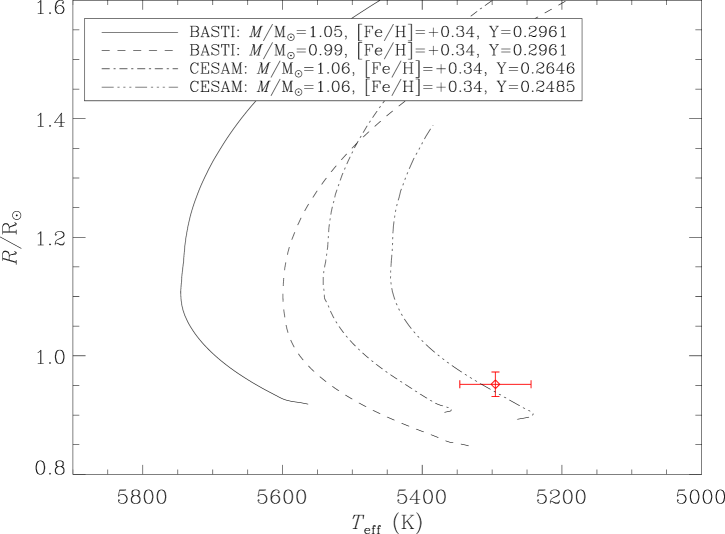
Figure 11.— Radius versus effective temperature with the position of the metal-rich main-sequence star HD 173701 shown as a red diamond. Lines compare BaSTI and CESAM evolutionary tracks with different masses and initial Helium fractions (see text). Note that each track starts at the zero-age main sequence (ZAMS). The determined mass and metallicity for HD 173701 are $M=1.05\pm 0.07\mbox{$M_{\sun}$}$ and $\rm{[Fe/H]}=+0.34\pm 0.06$.

4.3.2 HD 173701

Figure 11 shows the radius-$T_{\rm eff}$ diagram for HD 173701, a metal-rich main-sequence star with relatively well constrained properties. In this case, the agreement between BaSTI models and observations is poor. The difference can be reconciled with a $3-\sigma$ difference in mass and metallicity, i.e. the star is more metal-rich and less massive than implied from our observations. Indeed, the asteroseismic (but not model-independent) analyses by Mathur et al. (2012) and Silva Aguirre et al. (2012) imply a mass of $1.00\pm 0.01$ $M_{\sun}$  and $0.96\pm 0.04$ $M_{\sun}$  for HD 173701, respectively, which would significantly improve the agreement. We also note that the $\sim$100 K difference to the spectroscopic $T_{\rm eff}$ implies that the adopted metallicity may not be consistent with the interferometric $T_{\rm eff}$. However, as shown in Figure 11, even at the spectroscopic temperature of 5390 K the position of HD 173701 would still be slightly too cool for the mass determined from the interferometric radius and asteroseismic density. Additionally, adopting a lower $T_{\rm eff}$ in the spectroscopic analysis would result in a lower metallicity, and therefore enhance the disagreement between models and observations.

A more interesting possibility is that the physical assumptions in the evolutionary models need to be adjusted to reproduce the properties of this star. To test this, we have computed additional tracks using the 1D stellar evolution code CESAM (Morel & Lebreton, 2008). We use opacities from Ferguson et al. (2005) for the metal repartition by Asplund et al. (2009), and NACRE nuclear reaction rates are adapted from Angulo et al. (1999). The models include diffusion and gravitational settling, and convection is described using the mixing length theory by Böhm-Vitense (1958) with a solar calibrated value of 1.88. We have computed two models with the spectroscopically determined metallicity of [Fe/H] = 0.34 and a mass of 1.06$M_{\sun}$, once with solar-calibrated initial helium mass fraction $Y=0.2646$, and once with $Y=0.2485$, corresponding to the lower limit set by cosmological constraints. Figure 11 shows that changes in the initial chemical composition brings better agreement to our observations. Similar changes can be invoked by reducing the mixing-length parameter (see, e.g., Basu et al., 2010, 2012). Wright et al. (2004) list HD 173701 with a rotation period of 38 days and Ca H & K activity of $\log(R^{\prime}_{\rm HK})=-4.87$. Both the slower rotation period and solar-like activity do not seem to be compatible with a decreased convection efficiency (smaller mixing length parameter), which would be needed to bring the models in better agreement to our observations. Additionally, a sub-solar helium mass fraction for HD173701 does not seem to be compatible with the roughly linear helium-to-metal enrichment for metal-rich stars (Casagrande et al., 2007), although the scatter in this relation is large and studies of the Hyades have confirmed that stars can be depleted in helium and at the same time have a super-solar metallicity (Lebreton et al., 2001; Pinsonneault et al., 2003).

An alternative explanation could be related to inadequate modeling of stellar atmospheres for metal-rich stars. Systematics in these models would affect the bolometric flux and hence the determined effective temperature. Furthermore, systematic errors in the limb-darkening models for metal-rich stars would change the derived angular diameter, which influences the determined radius, mass and effective temperature. Detailed 3-D models by Bigot et al. (2006) for the metal-rich K-dwarf $\alpha$ Cen B showed less significant limb-darkening and hence slightly smaller diameters compared to simple 1-D models, while Chiavassa et al. (2010) found differences up to 3% for models of metal-poor giants. Such differences are expected to be enhanced in visibile wavelengths (such as the observations presented here) compared to infrared observations (Allende Prieto et al., 2002; Aufdenberg et al., 2005). Furthermore, comparisons of 1-D to 3-D models have also yielded higher fluxes for 3-D models, particularly at short wavelengths, which could lead to small inceases in the derived effective temperature (see, e.g., Aufdenberg et al., 2005; Casagrande, 2009). A higher effective temperature would bring better agreement to the evolutionary tracks and spectroscopic estimates. More detailed modeling will be needed to confirm if refined estimates of limb-darkening, taking into account the non-solar metallicity for HD 173701, can explain the observed differences.

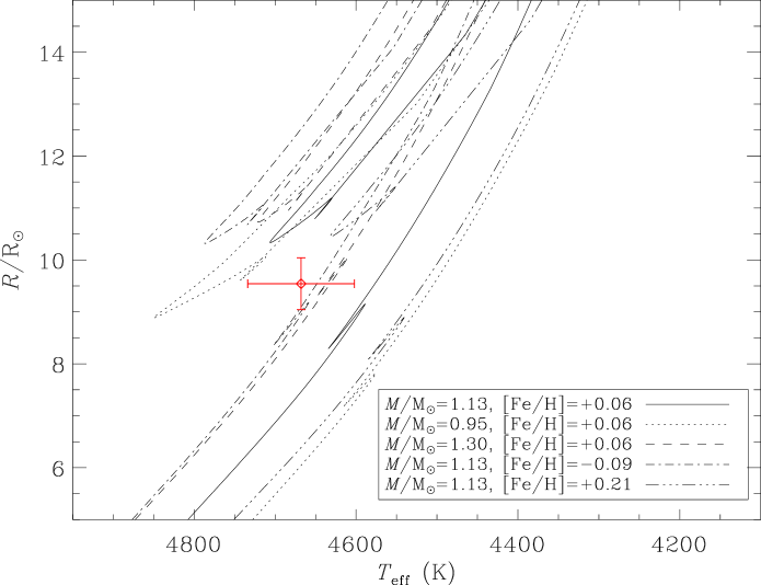
Figure 12.— Same as Figure 10 but for the red giant star HD 175955. The determined mass and metallicity for HD 175955 are $M=1.1\pm 0.2\mbox{$M_{\sun}$}$ and $\rm{[Fe/H]}=+0.06\pm 0.15$.

4.3.3 HD 175955

Figure 12 presents a model comparison for HD 175955, a red giant with a well constrained angular diameter and the most precise Hipparcos parallax. Gravity mode period spacings measured using asteroseismology have been used to classify this star as a H-shell burning, ascending red giant branch star (Bedding et al., 2011). Figure 12 shows that the measured temperature of HD 175955 is slightly hotter than the position of the ascending RGB tracks, but overall in good agreement with its determined mass and metallicity. Similar to HD 182736, a combination of the constraints presented here with detailed asteroseismic studies (such as the measurement of mixed mode rotational splittings to constrain the core rotation rate, see Beck et al., 2012) should allow a detailed theoretical study of the internal structure and evolution of this star.

4.3.4 Additional Notes

We note that for a few stars the derived stellar properties appear unphysical and are likely related to potential observational errors. For HD 175726, for example, the measured linear radius combined with the asteroseismic density implies a mass of $0.50\pm 0.03$$M_{\sun}$, which seems incompatible with its measured radius, temperature and solar-metallicity. Using the spectroscopically determined metallicity and the radius and temperature from interferometry, a comparison with BaSTI models indicates a mass of 1.07$M_{\sun}$, which would imply asteroseismic values of $\mbox{$\Delta\nu$}\sim 142\,\mbox{$\mu$Hz}$ and $\mbox{$\nu_{\rm max}$}\sim 3300$ $\mu$Hz. These values are significantly different than the results found by Mosser et al. (2009). The difference could be explained by an undetected companion causing a significant error in the parallax, or due to measurement errors in either the interferometric or the asteroseismic analysis. Unfortunately no CoRoT follow-up observations are planned for HD 175726, and hence a resolution of this discrepancy will have to await independent future observations.

The red giant HD 181827, on the other hand, has a large mass which is difficult to reconcile with evolutionary theory. Both the asteroseismic and interferometric constraints are solid, hence pointing to a potential problem with the Hipparcos parallax. Indeed, HD 181827 has the largest fractional parallax uncertainty in our sample (10%), leading to a large uncertainty on the radius and hence mass. We note that HD 181827 has been asteroseismically identified as a secondary clump star (Girardi, 1999; Bedding et al., 2011), corresponding to a massive ($\gtrsim 2\mbox{$M_{\sun}$}$) He-core burning red giant. Our result of a significantly higher mass for HD 181827 compared to typical red clump giants is hence qualitatively in agreement with its asteroseismically determined evolutionary state.

5. Conclusions

We have presented interferometrically measured angular diameters of 10 stars for which asteroseismic constraints are available from either the Kepler or CoRoT space telescopes. Combining these constraints with parallaxes, spectroscopy and bolometric fluxes, we present a full set of near model-independent fundamental properties for stars spanning in evolution from the main-sequence to the red clump. Our main conclusions from the derived properties are as follows:

1. Our measured angular diameters show good agreement with the surface-brightness relation by Kervella et al. (2004) and the IRFM coupled with asteroseismic constraints by Silva Aguirre et al. (2012), with an overall residual scatter of 5%. Our results seem to confirm that the relation by Kervella et al. (2004) and the method by Silva Aguirre et al. (2012) are also reasonably accurate for red giants.

2. A comparison of interferometric to asteroseismic radii calculated from scaling relations shows excellent agreement within the uncertainties. While the uncertainties for giants are large due to the uncertainties in the parallaxes, our results empirically prove that asteroseismic radii for unevolved stars using simple scaling relations are accurate to at least $4\%$. A test of the $\nu_{\rm max}$ scaling relation also shows no systematic deviations as a function of evolutionary state within the observational uncertainties.

3. A comparison of measured effective temperatures with estimates from modeling high-resolution spectra (mostly using the VWA method, see Bruntt et al., 2010) and from the photometric infrared flux method (see Casagrande et al., 2010) shows good agreement with mean deviations of $-22\pm 32$ K (with a scatter of 97 K) and $-58\pm 31$ K (with a scatter of 93 K), respectively, for stars between $T_{\rm eff}=4600-6200$ K. Some photometric calibrations show slight systematic deviations for red giants, presumably due to the more significant influence of reddening for these more distant stars.

4. A first comparison of our results with evolutionary models shows very good agreement for the subgiant HD 182736, while there appear to be some discrepancies for the metal-rich main-sequence star HD 173701. We speculate that these differences may be due to inadequate modeling of stellar atmospheres or limb-darkening for metal-rich stars, but note that more detailed theoretical studies will be needed to confirm this result.

While our study has demonstrated the potential of combining different constraints to test stellar model physics, it is clear that the overlap between the different techniques is still limited. This situation can be expected to be significantly improved with future projects such as the ground-based network SONG (Stellar Observations Network Group, Grundahl et al., 2006), which will deliver precise multi-site radial-velocity timeseries for asteroseismology and exoplanet studies of nearby stars. On the other hand, the planned European space mission Gaia (Perryman, 2003) will provide accurate parallaxes for stars down to $V<15$, while potential upgrades of interferometers such as the CHARA Array with adaptive optics will push the sensitivity limits of interferometric follow-up to fainter stars, therefore improving the overlap with Kepler and future space-based missions such as TESS (Transiting Exoplanet Survey Satellite, Ricker et al., 2009). The possibility of independently constraining radii, effective temperatures, masses and metallicities using asteroseismology, astrometry, interferometry and spectroscopy for a large ensemble of stars to study stellar physics as well as to characterize potentially habitable exoplanets is clearly the next step for continuing the exciting revolution induced by CoRoT and Kepler over the coming decades.

References

- Aerts et al. (2010) Aerts, C., Christensen-Dalsgaard, J., & Kurtz, D. W. 2010, Asteroseismology (Springer: Dodrecht)
- Allende Prieto et al. (2002) Allende Prieto, C., Asplund, M., García López, R. J., & Lambert, D. L. 2002, ApJ, 567, 544
- Alonso et al. (1995) Alonso, A., Arribas, S., & Martinez-Roger, C. 1995, A&A, 297, 197
- Alonso et al. (1999) Alonso, A., Arribas, S., & Martínez-Roger, C. 1999, A&AS, 140, 261
- Angulo et al. (1999) Angulo, C., et al. 1999, Nuclear Physics A, 656, 3
- Appourchaux et al. (2008) Appourchaux, T., et al. 2008, A&A, 488, 705
- Arentoft et al. (2008) Arentoft, T., et al. 2008, ApJ, 687, 1180
- Asplund et al. (2009) Asplund, M., Grevesse, N., Sauval, A. J., & Scott, P. 2009, ARA&A, 47, 481
- Aufdenberg et al. (2005) Aufdenberg, J. P., Ludwig, H.-G., & Kervella, P. 2005, ApJ, 633, 424
- Baglin et al. (2006a) Baglin, A., Michel, E., Auvergne, M., & The COROT Team. 2006a, in ESA Special Publication, Vol. 624, Proceedings of SOHO 18/GONG 2006/HELAS I, Beyond the spherical Sun
- Baglin et al. (2006b) Baglin, A., et al. 2006b, in 36th COSPAR Scientific Assembly, Vol. 36, 3749
- Baines et al. (2009) Baines, E. K., McAlister, H. A., ten Brummelaar, T. A., Sturmann, J., Sturmann, L., Turner, N. H., & Ridgway, S. T. 2009, ApJ, 701, 154
- Baines et al. (2008) Baines, E. K., McAlister, H. A., ten Brummelaar, T. A., Turner, N. H., Sturmann, J., Sturmann, L., Goldfinger, P. J., & Ridgway, S. T. 2008, ApJ, 680, 728
- Barban et al. (2007) Barban, C., et al. 2007, A&A, 468, 1033
- Barban et al. (2009) —. 2009, A&A, 506, 51
- Basu et al. (2010) Basu, S., Chaplin, W. J., & Elsworth, Y. 2010, ApJ, 710, 1596
- Basu et al. (2012) Basu, S., Verner, G. A., Chaplin, W. J., & Elsworth, Y. 2012, ApJ, 746, 76
- Bazot et al. (2011) Bazot, M., et al. 2011, A&A, 526, L4
- Beck et al. (2012) Beck, P. G., et al. 2012, Nature, 481, 55
- Bedding (2011) Bedding, T. R. 2011, ArXiv e-prints (arXiv:1107.1723)
- Bedding et al. (2004) Bedding, T. R., Kjeldsen, H., Butler, R. P., McCarthy, C., Marcy, G. W., O’Toole, S. J., Tinney, C. G., & Wright, J. T. 2004, ApJ, 614, 380
- Bedding et al. (2007) Bedding, T. R., et al. 2007, ApJ, 663, 1315
- Bedding et al. (2011) —. 2011, Nature, 471, 608
- Belkacem et al. (2011) Belkacem, K., Goupil, M. J., Dupret, M. A., Samadi, R., Baudin, F., Noels, A., & Mosser, B. 2011, A&A, 530, A142
- Benomar et al. (2009) Benomar, O., et al. 2009, A&A, 507, L13
- Bessell & Murphy (2012) Bessell, M., & Murphy, S. 2012, PASP, 124, 140
- Bessell (2000) Bessell, M. S. 2000, PASP, 112, 961
- Bessell et al. (1998) Bessell, M. S., Castelli, F., & Plez, B. 1998, A&A, 333, 231
- Bigot et al. (2006) Bigot, L., Kervella, P., Thévenin, F., & Ségransan, D. 2006, A&A, 446, 635
- Bigot et al. (2011) Bigot, L., et al. 2011, A&A, 534, L3
- Böhm-Vitense (1958) Böhm-Vitense, E. 1958, ZAp, 46, 108
- Borucki et al. (2010) Borucki, W. J., et al. 2010, Science, 327, 977
- Boyajian et al. (2009) Boyajian, T. S., et al. 2009, ApJ, 691, 1243
- Boyajian et al. (2012a) —. 2012a, ApJ, 746, 101
- Boyajian et al. (2012b) —. 2012b, ApJ, 757, 112
- Brasseur et al. (2010) Brasseur, C. M., Stetson, P. B., VandenBerg, D. A., Casagrande, L., Bono, G., & Dall’Ora, M. 2010, AJ, 140, 1672
- Brown & Gilliland (1994) Brown, T. M., & Gilliland, R. L. 1994, ARA&A, 32, 37
- Brown et al. (1991) Brown, T. M., Gilliland, R. L., Noyes, R. W., & Ramsey, L. W. 1991, ApJ, 368, 599
- Brown et al. (2011) Brown, T. M., Latham, D. W., Everett, M. E., & Esquerdo, G. A. 2011, AJ, 142, 112
- Bruntt (2009) Bruntt, H. 2009, A&A, 506, 235
- Bruntt et al. (2010) Bruntt, H., et al. 2010, MNRAS, 405, 1907
- Bruntt et al. (2012) —. 2012, MNRAS, 423, 122
- Cardelli et al. (1989) Cardelli, J. A., Clayton, G. C., & Mathis, J. S. 1989, ApJ, 345, 245
- Carrier & Bourban (2003) Carrier, F., & Bourban, G. 2003, A&A, 406, L23
- Carrier et al. (2005a) Carrier, F., Eggenberger, P., & Bouchy, F. 2005a, A&A, 434, 1085
- Carrier et al. (2005b) Carrier, F., Eggenberger, P., D’Alessandro, A., & Weber, L. 2005b, New A, 10, 315
- Casagrande (2009) Casagrande, L. 2009, Mem. Soc. Astron. Italiana, 80, 727
- Casagrande et al. (2007) Casagrande, L., Flynn, C., Portinari, L., Girardi, L., & Jimenez, R. 2007, MNRAS, 382, 1516
- Casagrande et al. (2010) Casagrande, L., Ramírez, I., Meléndez, J., Bessell, M., & Asplund, M. 2010, A&A, 512, A54
- Castelli & Kurucz (2003) Castelli, F., & Kurucz, R. L. 2003, in IAU Symposium, Vol. 210, Modelling of Stellar Atmospheres, ed. N. Piskunov, W. W. Weiss, & D. F. Gray, 20P
- Castelli & Kurucz (2004) Castelli, F., & Kurucz, R. L. 2004, ArXiv e-prints (arXiv:0405087)
- Chaplin et al. (2011) Chaplin, W. J., et al. 2011, Science, 332, 213
- Chiavassa et al. (2012) Chiavassa, A., Bigot, L., Kervella, P., Matter, A., Lopez, B., Collet, R., Magic, Z., & Asplund, M. 2012, A&A, 540, A5
- Chiavassa et al. (2010) Chiavassa, A., Collet, R., Casagrande, L., & Asplund, M. 2010, A&A, 524, A93
- Christensen-Dalsgaard (2004) Christensen-Dalsgaard, J. 2004, Sol. Phys., 220, 137
- Claret & Bloemen (2011) Claret, A., & Bloemen, S. 2011, A&A, 529, A75
- Code et al. (1976) Code, A. D., Bless, R. C., Davis, J., & Brown, R. H. 1976, ApJ, 203, 417
- Cohen et al. (2003) Cohen, M., Wheaton, W. A., & Megeath, S. T. 2003, AJ, 126, 1090
- Colina et al. (1996) Colina, L., Bohlin, R. C., & Castelli, F. 1996, AJ, 112, 307
- Creevey et al. (2012) Creevey, O. L., et al. 2012, A&A, 545, A17
- Cunha et al. (2007) Cunha, M. S., et al. 2007, A&A Rev., 14, 217
- Cutri et al. (2003) Cutri, R. M., et al. 2003, 2MASS All Sky Catalog of point sources., ed. Cutri, R. M., Skrutskie, M. F., van Dyk, S., Beichman, C. A., Carpenter, J. M., Chester, T., Cambresy, L., Evans, T., Fowler, J., Gizis, J., Howard, E., Huchra, J., Jarrett, T., Kopan, E. L., Kirkpatrick, J. D., Light, R. M., Marsh, K. A., McCallon, H., Schneider, S., Stiening, R., Sykes, M., Weinberg, M., Wheaton, W. A., Wheelock, S., & Zacarias, N.
- De Ridder et al. (2006) De Ridder, J., Barban, C., Carrier, F., Mazumdar, A., Eggenberger, P., Aerts, C., Deruyter, S., & Vanautgaerden, J. 2006, A&A, 448, 689
- De Ridder et al. (2009) De Ridder, J., et al. 2009, Nature, 459, 398
- Deheuvels & Michel (2011) Deheuvels, S., & Michel, E. 2011, A&A, 535, A91
- Deheuvels et al. (2012) Deheuvels, S., et al. 2012, ApJ, 756, 19
- Demarque et al. (1986) Demarque, P., Guenther, D. B., & van Altena, W. F. 1986, ApJ, 300, 773
- Derekas et al. (2011) Derekas, A., et al. 2011, Science, 332, 216
- Domiciano de Souza et al. (2002) Domiciano de Souza, A., Vakili, F., Jankov, S., Janot-Pacheco, E., & Abe, L. 2002, A&A, 393, 345
- Drimmel et al. (2003) Drimmel, R., Cabrera-Lavers, A., & López-Corredoira, M. 2003, A&A, 409, 205
- Ferguson et al. (2005) Ferguson, J. W., Alexander, D. R., Allard, F., Barman, T., Bodnarik, J. G., Hauschildt, P. H., Heffner-Wong, A., & Tamanai, A. 2005, ApJ, 623, 585
- Flower (1996) Flower, P. J. 1996, ApJ, 469, 355
- Frasca et al. (2003) Frasca, A., Alcalá, J. M., Covino, E., Catalano, S., Marilli, E., & Paladino, R. 2003, A&A, 405, 149
- Frasca et al. (2006) Frasca, A., Guillout, P., Marilli, E., Freire Ferrero, R., Biazzo, K., & Klutsch, A. 2006, A&A, 454, 301
- Fuhrmann et al. (1997) Fuhrmann, K., Pfeiffer, M., Frank, C., Reetz, J., & Gehren, T. 1997, A&A, 323, 909
- Fusi-Pecci & Renzini (1976) Fusi-Pecci, F., & Renzini, A. 1976, A&A, 46, 447
- Gai et al. (2011) Gai, N., Basu, S., Chaplin, W. J., & Elsworth, Y. 2011, ApJ, 730, 63
- García et al. (2011) García, R. A., et al. 2011, MNRAS, 414, L6
- Gilliland et al. (2010a) Gilliland, R. L., et al. 2010a, ApJ, 713, L160
- Gilliland et al. (2010b) —. 2010b, PASP, 122, 131
- Girardi (1999) Girardi, L. 1999, MNRAS, 308, 818
- Grevesse & Noels (1993) Grevesse, N., & Noels, A. 1993, in Origin and Evolution of the Elements, ed. N. Prantzos, E. Vangioni-Flam, & M. Casse, 15–25
- Grundahl et al. (2006) Grundahl, F., Kjeldsen, H., Frandsen, S., Andersen, M., Bedding, T., Arentoft, T., & Christensen-Dalsgaard, J. 2006, Mem. Soc. Astron. Italiana, 77, 458
- Gustafsson et al. (2008) Gustafsson, B., Edvardsson, B., Eriksson, K., Jørgensen, U. G., Nordlund, Å., & Plez, B. 2008, A&A, 486, 951
- Guzik et al. (2011) Guzik, J. A., et al. 2011, ArXiv e-prints (arXiv:1110.2120)
- Hanbury Brown et al. (1974) Hanbury Brown, R., Davis, J., Lake, R. J. W., & Thompson, R. J. 1974, MNRAS, 167, 475
- Hekker et al. (2009) Hekker, S., et al. 2009, A&A, 506, 465
- Hekker et al. (2011a) —. 2011a, A&A, 530, A100
- Hekker et al. (2011b) —. 2011b, MNRAS, 414, 2594
- Hekker et al. (2011c) —. 2011c, A&A, 525, A131
- Hekker et al. (2012) —. 2012, A&A, 544, A90
- Høg et al. (2000) Høg, E., et al. 2000, A&A, 355, L27
- Huber et al. (2009) Huber, D., Stello, D., Bedding, T. R., Chaplin, W. J., Arentoft, T., Quirion, P.-O., & Kjeldsen, H. 2009, Communications in Asteroseismology, 160, 74
- Huber et al. (2011) Huber, D., et al. 2011, ApJ, 743, 143
- Huber et al. (2012) —. 2012, MNRAS, 423, L16
- Ireland et al. (2008) Ireland, M. J., et al. 2008, in Presented at the Society of Photo-Optical Instrumentation Engineers (SPIE) Conference, Vol. 7013, Society of Photo-Optical Instrumentation Engineers (SPIE) Conference Series
- Jenkins et al. (2010) Jenkins, J. M., et al. 2010, ApJ, 713, L120
- Kallinger et al. (2010a) Kallinger, T., Gruberbauer, M., Guenther, D. B., Fossati, L., & Weiss, W. W. 2010a, A&A, 510, A106
- Kallinger et al. (2008) Kallinger, T., et al. 2008, A&A, 478, 497
- Kallinger et al. (2010b) —. 2010b, A&A, 522, A1
- Kallinger et al. (2010c) —. 2010c, A&A, 509, A77
- Kervella et al. (2004) Kervella, P., Thévenin, F., Di Folco, E., & Ségransan, D. 2004, A&A, 426, 297
- Kjeldsen & Bedding (1995) Kjeldsen, H., & Bedding, T. R. 1995, A&A, 293, 87
- Kjeldsen et al. (2003) Kjeldsen, H., et al. 2003, AJ, 126, 1483
- Kjeldsen et al. (2005) —. 2005, ApJ, 635, 1281
- Koch et al. (2010) Koch, D. G., et al. 2010, ApJ, 713, L79
- Kovtyukh et al. (2003) Kovtyukh, V. V., Soubiran, C., Belik, S. I., & Gorlova, N. I. 2003, A&A, 411, 559
- Lebreton et al. (2001) Lebreton, Y., Fernandes, J., & Lejeune, T. 2001, A&A, 374, 540
- Lefever et al. (2010) Lefever, K., Puls, J., Morel, T., Aerts, C., Decin, L., & Briquet, M. 2010, A&A, 515, A74
- Mathur et al. (2012) Mathur, S., et al. 2012, ApJ, 749, 152
- Mazumdar et al. (2009) Mazumdar, A., et al. 2009, A&A, 503, 521
- Mermilliod et al. (1997) Mermilliod, J.-C., Mermilliod, M., & Hauck, B. 1997, A&AS, 124, 349
- Metcalfe et al. (2012) Metcalfe, T. S., et al. 2012, ApJ, 748, L10
- Miglio (2012) Miglio, A. 2012, in Red Giants as Probes of the Structure and Evolution of the Milky Way, ed. A. Miglio, J. Montalbán, & A. Noels, ApSS Proceedings
- Mishenina et al. (2004) Mishenina, T. V., Soubiran, C., Kovtyukh, V. V., & Korotin, S. A. 2004, A&A, 418, 551
- Molenda-Żakowicz et al. (2009) Molenda-Żakowicz, J., Jerzykiewicz, M., & Frasca, A. 2009, Acta Astron., 59, 213
- Monteiro et al. (1996) Monteiro, M. J. P. F. G., Christensen-Dalsgaard, J., & Thompson, M. J. 1996, A&A, 307, 624
- Morel & Lebreton (2008) Morel, P., & Lebreton, Y. 2008, Ap&SS, 316, 61
- Mosser et al. (2009) Mosser, B., et al. 2009, A&A, 506, 33
- Mosser et al. (2010) —. 2010, A&A, 517, A22
- North et al. (2007) North, J. R., et al. 2007, MNRAS, 380, L80
- O’Donnell (1994) O’Donnell, J. E. 1994, ApJ, 422, 158
- Perryman (2003) Perryman, M. A. C. 2003, in Astronomical Society of the Pacific Conference Series, Vol. 298, GAIA Spectroscopy: Science and Technology, ed. U. Munari, 3
- Perryman & ESA (1997) Perryman, M. A. C., & ESA, eds. 1997, ESA Special Publication, Vol. 1200, The HIPPARCOS and TYCHO catalogues. Astrometric and photometric star catalogues derived from the ESA HIPPARCOS Space Astrometry Mission
- Piau et al. (2011) Piau, L., Kervella, P., Dib, S., & Hauschildt, P. 2011, A&A, 526, A100
- Pietrinferni et al. (2004) Pietrinferni, A., Cassisi, S., Salaris, M., & Castelli, F. 2004, ApJ, 612, 168
- Pinsonneault et al. (2012) Pinsonneault, M. H., An, D., Molenda-Żakowicz, J., Chaplin, W. J., Metcalfe, T. S., & Bruntt, H. 2012, ApJS, 199, 30
- Pinsonneault et al. (2003) Pinsonneault, M. H., Terndrup, D. M., Hanson, R. B., & Stauffer, J. R. 2003, ApJ, 598, 588
- Prugniel et al. (2007) Prugniel, P., Soubiran, C., Koleva, M., & Le Borgne, D. 2007, ArXiv e-prints (arXiv:0703658)
- Ramírez & Allende Prieto (2011) Ramírez, I., & Allende Prieto, C. 2011, ApJ, 743, 135
- Ramírez & Meléndez (2005) Ramírez, I., & Meléndez, J. 2005, ApJ, 626, 465
- Ricker et al. (2009) Ricker, G. R., et al. 2009, in Bulletin of the American Astronomical Society, Vol. 41, American Astronomical Society Meeting Abstracts 213, 403.01
- Santos et al. (2004) Santos, N. C., Israelian, G., & Mayor, M. 2004, A&A, 415, 1153
- Silva Aguirre et al. (2011) Silva Aguirre, V., et al. 2011, ApJ, 740, L2
- Silva Aguirre et al. (2012) —. 2012, ApJ, 757, 99
- Skrutskie et al. (2006) Skrutskie, M. F., et al. 2006, AJ, 131, 1163
- Söderhjelm (1999) Söderhjelm, S. 1999, A&A, 341, 121
- Sousa et al. (2006) Sousa, S. G., Santos, N. C., Israelian, G., Mayor, M., & Monteiro, M. J. P. F. G. 2006, A&A, 458, 873
- Sousa et al. (2008) Sousa, S. G., et al. 2008, A&A, 487, 373
- Stello et al. (2009a) Stello, D., Chaplin, W. J., Basu, S., Elsworth, Y., & Bedding, T. R. 2009a, MNRAS, 400, L80
- Stello et al. (2009b) Stello, D., et al. 2009b, ApJ, 700, 1589
- Teixeira et al. (2009) Teixeira, T. C., et al. 2009, A&A, 494, 237
- ten Brummelaar et al. (2005) ten Brummelaar, T. A., et al. 2005, ApJ, 628, 453
- Thygesen et al. (2012) Thygesen, A. O., et al. 2012, A&A, 543, A160
- Torres (2010) Torres, G. 2010, AJ, 140, 1158
- Torres et al. (2012) Torres, G., Fischer, D. A., Sozzetti, A., Buchhave, L. A., Winn, J. N., Holman, M. J., & Carter, J. A. 2012, ApJ, 757, 161
- Trampedach & Stein (2011) Trampedach, R., & Stein, R. F. 2011, ApJ, 731, 78
- Ulrich (1986) Ulrich, R. K. 1986, ApJ, 306, L37
- Valenti & Fischer (2005) Valenti, J. A., & Fischer, D. A. 2005, ApJS, 159, 141
- van Belle (1999) van Belle, G. T. 1999, PASP, 111, 1515
- van Belle & von Braun (2009) van Belle, G. T., & von Braun, K. 2009, ApJ, 694, 1085
- van Leeuwen (2007) van Leeuwen, F. 2007, A&A, 474, 653
- VandenBerg et al. (2010) VandenBerg, D. A., Casagrande, L., & Stetson, P. B. 2010, AJ, 140, 1020
- Verner et al. (2011) Verner, G. A., et al. 2011, MNRAS, 415, 3539
- von Braun et al. (2011a) von Braun, K., et al. 2011a, ApJ, 740, 49
- von Braun et al. (2011b) —. 2011b, ApJ, 729, L26
- White et al. (2011) White, T. R., Bedding, T. R., Stello, D., Christensen-Dalsgaard, J., Huber, D., & Kjeldsen, H. 2011, ApJ, 743, 161
- Wright et al. (2004) Wright, J. T., Marcy, G. W., Butler, R. P., & Vogt, S. S. 2004, ApJS, 152, 261