Dispersing billiards with moving scatterers

Abstract.

We propose a model of Sinai billiards with moving scatterers, in which the locations and shapes of the scatterers may change by small amounts between collisions. Our main result is the exponential loss of memory of initial data at uniform rates, and our proof consists of a coupling argument for non-stationary compositions of maps similar to classical billiard maps. This can be seen as a prototypical result on the statistical properties of time-dependent dynamical systems.

1. Introduction

1.1. Motivation

The physical motivation for our paper is a setting in which a finite number of larger and heavier particles move about slowly as they are bombarded by a large number of lightweight (gas) particles. Following the language of billiards, we refer to the heavy particles as scatterers. In classical billiards theory, scatterers are assumed to be stationary, an assumption justified by first letting the ratios of masses of heavy-to-light particles tend to infinity. We do not fix the scatterers here. Indeed the system may be open — gas particles can be injected or ejected, heated up or cooled down. We consider a window of observation $[0,T],\ T\leq\infty$, and assume that during this time interval the total energy stays uniformly below a constant value $E>0$. This places an upper bound proportional to $\sqrt{E}$ on the translational and rotational speeds of the scatterers. The constant of proportionality depends inversely on the masses and moments of inertia of the scatterers. Suppose the scatterers are also pairwise repelling due to an interaction with a short but positive effective range, such as a weak Coulomb force, whose strength tends to infinity with the inverse of the distance. The distance between any pair of scatterers has then a lower bound, which in the Coulomb case is proportional to $1/E$. In brief, fixing a maximum value for the total energy $E$, the scatterers are guaranteed to be uniformly bounded away from each other; and assuming that the ratios of masses are sufficiently large, the scatterers will move arbitrarily slowly. Our goal is to study the dynamics of a tagged gas particle in such a system on the time interval $[0,T]$. As a simplification we assume our tagged particle is passive: it is massless, does not interact with the other light particles, and does not interfere with the motion of the scatterers. It experiences an elastic collision each time it meets a scatterer, and moves on with its own energy unchanged. This model was proposed in the paper [16].

The setting above is an example of a time-dependent dynamical system. Much of dynamical systems theory as it exists today is concerned with autonomous systems, i.e., systems for which the rules of the dynamics remain constant through time. Non-autonomous systems studied include those driven by a time-periodic or random forcing (as described by SDEs), or more generally, systems driven by another autonomous dynamical system (as in a skew-product setup). For time-varying systems without any assumption of periodicity or stationarity, even the formulation of results poses obvious mathematical challenges, yet many real-world systems are of this type. Thus while the moving scatterers model above is of independent interest, we had another motive for undertaking the present project: we wanted to use this prototypical example to catch a glimpse of the challenges ahead, and at the same time to identify techniques of stationary theory that carry over to time-dependent systems.

1.2. Main results and issues

We focus in this paper on the evolution of densities. Let $\rho_{0}$ be an initial distribution, and $\rho_{t}$ its time evolution. In the case of an autonomous system with good statistical properties, one would expect $\rho_{t}$ to tend to the system’s natural invariant distribution (e.g. SRB measure) as $t\to\infty$. The question is: How quickly is $\rho_{0}$ “forgotten”? Since “forgetting” the features of an initial distribution is generally associated with mixing of the dynamical system, one may pose the question as follows: Given two initial distributions $\rho_{0}$ and $\rho^{\prime}_{0}$, how quickly does $|\rho_{t}-\rho^{\prime}_{t}|$ tend to zero (in some measure of distance)? In the time-dependent case, $\rho_{t}$ and $\rho^{\prime}_{t}$ may never settle down, as the rules of the dynamics may be changing perpetually. Nevertheless the question continues to makes sense. We say a system has exponential memory loss if $|\rho_{t}-\rho^{\prime}_{t}|$ decreases exponentially with time.

Since memory loss is equivalent to mixing for a fixed map, a natural setting with exponential memory loss for time-dependent sequences is when the maps to be composed have, individually, strong mixing properties, and the rules of the dynamics, or the maps to be composed, vary slowly. (In the case of continuous time, this is equivalent to the vector field changing very slowly.) In such a setting, we may think of $\rho_{t}$ above as slowly varying as well. Furthermore, in the case of exponential loss of memory, we may view these probability distributions as representing, after an initial transient, quasi-stationary states.

Our main result in this paper is the exponential memory loss of initial data for the collision maps of 2D models of the type described in Section 1.1, where the scatterers are assumed to be moving very slowly. Precise results are formulated in Section 2. Billiard maps with fixed, convex scatterers are known to have exponential correlation decay; thus the setting in Section 1.1 is a natural illustration of the scenario in the last paragraph. (Incidentally, when the source and target configurations differ, the collision map does not necessarily preserve the usual invariant measure).

If we were to iterate a single map long enough for exponential mixing to set in, then change the map ever so slightly so as not to disturb the convergence in $|\rho_{t}-\rho^{\prime}_{t}|$ already achieved, and iterate the second map for as long as needed before making an even smaller change, and so on, then exponential loss of memory for the sequence is immediate for as long as all the maps involved are individually exponentially mixing. This is not the type of result we are after. A more meaningful result — and this is what we will prove — is one in which one identifies a space of dynamical systems and an upper bound in the speed with which the sequence is allowed to vary, and prove exponential memory loss for any sequence in this space that varies slowly enough. This involves more than the exponential mixing property of individual maps; the class of maps in question has to satisfy a uniform mixing condition for slowly-varying compositions. This in some sense is the crux of the matter.

A technical but fundamental issue has to do with stable and unstable directions, the staples of hyperbolic dynamics. In time-dependent systems with slowly-varying parameters, approximate stable and unstable directions can be defined, but they depend on the time interval of interest, e.g., which direction is contracting depends on how long one chooses to look. Standard dynamical tools have to be adapted to the new setting of non-stationary sequences; consequently technical estimates of single billiard maps have to be re-examined as well.

1.3. Relevant works

Our work lies at the confluence of the following two sets of results:

The study of statistical properties of billiard maps in the case of fixed convex scatterers was pioneered by Sinai et al [17, 3, 4]. The result for exponential correlation decay was first proved in [20]; another proof using a coupling argument is given in [6]. Our exposition here follows closely that in [6]. Coupling, which is the main tool of the present paper, is a standard technique in probability. To our knowledge it was imported into hyperbolic dynamical systems in [21]. The very convenient formulation in [6] was first used in [8]. (Despite appearing in 2009, the latter circulated as a preprint already in 2004.) We refer the reader to [10], which contains a detailed exposition of this and many other important technical facts related to billiards.

The paper [16] proved exponential loss of memory for expanding maps and for one-dimensional piecewise expanding maps with slowly varying parameters. An earlier study in the same spirit is [13]. A similar result was obtained for topologically transitive Anosov diffeomorphisms in two dimensions in [18] and for piecewise expanding maps in higher dimensions in [12]. We mention also [2], where exponential memory loss was established for arbitrary sequences of finitely many toral automorphisms satisfying a common-cone condition. Recent central-limit-type results in the time-dependent setting can be found in [11, 15, 19].

1.4. About the exposition

One of the goals of this paper is to stress the (strong) similarities between stationary dynamics and their time-dependent counterparts, and to highlight at the same time the new issues that need to be addressed. For this reason, and also to keep the length of the manuscript reasonable, we have elected to omit the proofs of some technical preliminaries for which no substantial modifications are needed from the fixed-scatterers case, referring the reader instead to [10]. We do not know to what degree we have succeeded, but we have tried very hard to make transparent the logic of the argument, in the hope that it will be accessible to a wider audience. The main ideas are contained in Section 5.

The paper is organized as follows. In Section 2 we describe the model in detail, after which we immediately state our main results in a form as accessible as possible, leaving generalizations for later. Theorems 1–3 of Section 2 are the main results of this paper, and Theorem 4 is a more technical formulation which easily implies the other two. Sections 3 and 4 contain a collection of facts about dispersing billiard maps that are easily adapted to the time-dependent case. Section 5 gives a nearly complete outline of the proof of Theorem 4. In Section 6 we continue with technical preliminaries necessary for a rigorous proof of that theorem. Unlike Sections 3 and 4, more stringent conditions on the speeds at which the scatterers are allowed to move are needed for the results in Section 6. In Section 7 we prove Theorem 4 in the special case of initial distributions supported on countably many curves, and in Section 8 we prove the extension of Theorem 4 to more general settings. Finally, we collect in the Appendix some proofs which are deferred to the end in order not to disrupt the flow of the presentation in the body of the text.

2. Precise statement of main results

2.1. Setup

We fix here a space of scatterer configurations, and make precise the definition of billiard maps with possibly different source and target configurations.

Throughout this paper, the physical space of our system is the $2$-torus ${\mathbb{T}}^{2}$. We assume, to begin with (this condition will be relaxed later on), that the number of scatterers as well as their sizes and shapes are fixed, though rigid rotations and translations are permitted. Formally, let $B_{1},\dots,B_{\mathfrak{s}}$ be pairwise disjoint closed convex domains in $\mathbb{R}^{2}$ with $C^{3}$ boundaries of strictly positive curvature. In the interior of each $B_{i}$ we fix a reference point $c_{i}$ and a unit vector $u_{i}$ at $c_{i}$. A configuration $\mathcal{K}$ of $\{B_{1},\dots,B_{\mathfrak{s}}\}$ in ${\mathbb{T}}^{2}$ is an embedding of $\cup_{i=1}^{\mathfrak{s}}B_{i}$ into ${\mathbb{T}}^{2}$, one that maps each $B_{i}$ isometrically onto a set we call $\mathbf{B}_{i}$. Thus $\mathcal{K}$ can be identified with a point $(\mathbf{c}_{i},\mathbf{u}_{i})_{i=1}^{\mathfrak{s}}\in{({\mathbb{T}}^{2}\times{\mathbb{S}}^{1})}^{\mathfrak{s}}$, $\mathbf{c}_{i}$ and $\mathbf{u}_{i}$ being images of $c_{i}$ and $u_{i}$. The space of configurations $\mathbb{K}_{0}$ is the subset of ${({\mathbb{T}}^{2}\times{\mathbb{S}}^{1})}^{\mathfrak{s}}$ for which the $\mathbf{B}_{i}$ are pairwise disjoint and every half-line in ${\mathbb{T}}^{2}$ meets a scatterer non-tangentially. More conditions will be imposed on $\mathcal{K}$ later on. The set $\mathbb{K}_{0}$ inherits the Euclidean metric from ${({\mathbb{T}}^{2}\times{\mathbb{S}}^{1})}^{\mathfrak{s}}$, and the $\varepsilon$-neighborhood of $\mathcal{K}$ is denoted by $\mathcal{N}_{\varepsilon}(\mathcal{K})$.

Given a configuration $\mathcal{K}\in{\mathbb{K}}_{0}$, let $\tau^{\min}_{\mathcal{K}}$ be the shortest length of a line segment in ${\mathbb{T}}^{2}\setminus\cup_{i=1}^{\mathfrak{s}}\mathbf{B}_{i}$ which originates and terminates (possibly tangentially) in the set $\cup_{i=1}^{\mathfrak{s}}\partial\mathbf{B}_{i}$, and let $\tau^{\max}_{\mathcal{K}}$ be the supremum of the lengths of all line segments in the closure of ${\mathbb{T}}^{2}\setminus\cup_{i=1}^{\mathfrak{s}}\mathbf{B}_{i}$ which originate and terminate non-tangentially in the set $\cup_{i=1}^{\mathfrak{s}}\partial\mathbf{B}_{i}$ (this segment may meet the scatterers tangentially between its endpoints). As a function of $\mathcal{K}$, $\tau^{\min}_{\mathcal{K}}$ is continuous, but $\tau^{\max}_{\mathcal{K}}$ in general is only upper semi-continuous. Notice that $0<\tau^{\min}_{\mathcal{K}}<\tau^{\max}_{\mathcal{K}}\leq\infty$.

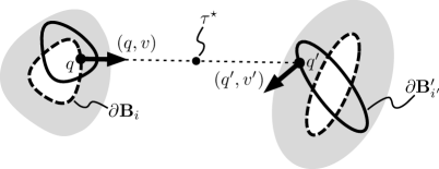
Figure 1. Rules of the dynamics. Scatterers in source configuration $\mathcal{K}$ and target configuration $\mathcal{K}^{\prime}$ are drawn in dashed and solid line, respectively. A particle shoots off the boundary of a scatterer $\mathbf{B}_{i}$ at the point $q$ with unit velocity $v$ and exits the gray buffer zone $\mathbf{B}_{i,\beta}\setminus\mathbf{B}_{i}$. Before it re-enters the buffer zone of any scatterer $\mathbf{B}_{j}$, the configuration is switched instantaneously from $\mathcal{K}$ to $\mathcal{K}^{\prime}$ at some time $\tau^{\star}$ during mid-flight. The particle then hits the boundary of a scatterer $\mathbf{B}_{i^{\prime}}^{\prime}$ elastically at the point $q^{\prime}$, resulting in post-collision velocity $v^{\prime}$.

A basic question is: Given $\mathcal{K},\mathcal{K}^{\prime}\in{\mathbb{K}}_{0}$, is there always a well-defined billiard map (analogous to classical billiard maps) with source configuration $\mathcal{K}$ and target configuration $\mathcal{K}^{\prime}$? That is to say, if $\mathbf{B}_{1},\dots,\mathbf{B}_{\mathfrak{s}}$ are the scatterers in configuration $\mathcal{K}$, and $\mathbf{B}_{1}^{\prime},\dots,\mathbf{B}_{\mathfrak{s}}^{\prime}$ are the corresponding scatterers in $\mathcal{K}^{\prime}$, is there a well defined mapping

$$\mathbf{F}_{\mathcal{K}^{\prime},\mathcal{K}}:T^{+}_{1}(\cup_{i=1}^{\mathfrak{s}}\partial\mathbf{B}_{i})\to T^{+}_{1}(\cup_{i=1}^{\mathfrak{s}}\partial\mathbf{B}^{\prime}_{i})$$

where $T^{+}_{1}(\cup_{i=1}^{\mathfrak{s}}\partial\mathbf{B}_{i})$ is the set of $(q,v)$ such that $q\in\cup_{i=1}^{\mathfrak{s}}\partial\mathbf{B}_{i}$ and $v$ is a unit vector at $q$ pointing into the region ${\mathbb{T}}^{2}\setminus\cup_{i=1}^{\mathfrak{s}}\mathbf{B}_{i}$, and similarly for $T^{+}_{1}(\cup_{i=1}^{\mathfrak{s}}\partial\mathbf{B}^{\prime}_{i})$? Is the map $\mathbf{F}_{\mathcal{K}^{\prime},\mathcal{K}}$ uniquely defined, or does it depend on when the changeover from $\mathcal{K}$ to $\mathcal{K}^{\prime}$ occurs? The answer can be very general, but let us confine ourselves to the special case where $\mathcal{K}^{\prime}$ is very close to $\mathcal{K}$ and the changeover occurs when the particle is in “mid-flight” (to avoid having scatterers land on top of the particle, or meet it at the exact moment of the changeover).

To do this systematically, we introduce the idea of a buffer zone. For $\beta>0$, we let $\mathbf{B}_{i,\beta}\subset{\mathbb{T}}^{2}$ denote the $\beta$-neighborhood of $\mathbf{B}_{i}$, and define $\tau^{\textrm{esc}}_{\beta}$, the escape time from the $\beta$-neighborhood of $\cup_{i}\mathbf{B}_{i}$, to be the maximum length of a line in $\cup_{i=1}^{\mathfrak{s}}(\mathbf{B}_{i,\beta}\setminus\mathbf{B}_{i})$ connecting $\cup_{i=1}^{\mathfrak{s}}\partial\mathbf{B}_{i}$ to $\cup_{i=1}^{\mathfrak{s}}\partial(\mathbf{B}_{i,\beta})$. We then fix a value of $\beta>0$ small enough that $\tau^{\textrm{esc}}_{\beta}<\tau^{\min}_{\mathcal{K}}-\beta$, and require that $\mathbf{B}_{i}^{\prime}\subset\mathbf{B}_{i,\beta}$ for each $i=1,\dots,\mathfrak{s}$. Notice that $\beta<\tau^{\textrm{esc}}_{\beta}$, so that $\beta<\tau^{\min}_{\mathcal{K}}/2$, implying in particular that the neighborhoods $\mathbf{B}_{i,\beta}$ are pairwise disjoint. For a particle starting from $\cup_{i=1}^{\mathfrak{s}}\partial\mathbf{B}_{i}$, its trajectory is guaranteed to be outside of $\cup_{i=1}^{\mathfrak{s}}\mathbf{B}_{i,\beta}$ during the time interval $(\tau^{\textrm{esc}}_{\beta},\tau^{\min}_{\mathcal{K}}-\beta)$: reaching $\cup_{i=1}^{\mathfrak{s}}\mathbf{B}_{i,\beta}$ before time $\tau^{\min}_{\mathcal{K}}-\beta$ would contradict the definition of $\tau^{\min}_{\mathcal{K}}$. We permit the configuration change to take place at any time $\tau^{\star}\in(\tau^{\textrm{esc}}_{\beta},\tau^{\min}_{\mathcal{K}}-\beta)$. Notice that $\tau^{\textrm{esc}}_{\beta}$ depends only on the shapes of the scatterers, not their configuration, and that the billiard trajectory starting from $\cup_{i}\partial\mathbf{B}_{i}$ and ending in $\cup_{i}\partial\mathbf{B}^{\prime}_{i}$ does not depend on the precise moment $\tau^{\star}$ at which the configuration is updated. For the billiard map $\mathbf{F}_{\mathcal{K}^{\prime},\mathcal{K}}$ to be defined, every particle trajectory starting from $\cup_{i=1}^{\mathfrak{s}}\partial\mathbf{B}_{i}$ must meet a scatterer in $\mathcal{K}^{\prime}$. This is guaranteed by $\mathcal{K}^{\prime}\in{\mathbb{K}}_{0}$, due to the requirement that any half-line intersects a scatterer boundary.

To summarize, we have argued that given $\mathcal{K},\mathcal{K}^{\prime}\in{\mathbb{K}}_{0}$, there is a canonical way to define $\mathbf{F}_{\mathcal{K}^{\prime},\mathcal{K}}$ if $\mathbf{B}_{i}^{\prime}\subset\mathbf{B}_{i,\beta}$ for all $i$ where $\beta=\beta(\tau^{\min}_{\mathcal{K}})>0$ depends only on $\tau^{\min}_{\mathcal{K}}$ (and the curvatures of the $B_{i}$), and the flight time $\tau_{\mathcal{K}^{\prime},\mathcal{K}}$ satisfies $\tau_{\mathcal{K}^{\prime},\mathcal{K}}\geq\tau^{\min}_{\mathcal{K}}-\beta\geq\tau^{\min}_{\mathcal{K}}/2$.

Now we would like to have all the $\mathbf{F}_{\mathcal{K}^{\prime},\mathcal{K}}$ operate on a single phase space $\mathcal{M}$, so that our time-dependent billiard system defined by compositions of these maps can be studied in a way analogous to iterated classical billiard maps. As usual, we let $\Gamma_{i}$ be a fixed clockwise parametrization by arclength of $\partial B_{i}$, and let

$$\mathcal{M}=\cup_{i}\mathcal{M}_{i}\quad\text{with}\quad\mathcal{M}_{i}=\Gamma_{i}\times[-\pi/2,\pi/2].$$

Recall that each $\mathcal{K}\in{\mathbb{K}}$ is defined by an isometric embedding of $\cup_{i=1}^{\mathfrak{s}}B_{i}$ into ${\mathbb{T}}^{2}$. This embedding extends to a neighborhood of $\cup_{i=1}^{\mathfrak{s}}B_{i}\subset\mathbb{R}^{2}$, inducing a diffeomorphism $\Phi_{\mathcal{K}}:\mathcal{M}\to T^{+}_{1}(\cup_{i=1}^{\mathfrak{s}}\partial\mathbf{B}_{i})$. For $\mathcal{K},\mathcal{K}^{\prime}$ for which $\mathbf{F}_{\mathcal{K}^{\prime},\mathcal{K}}$ is defined then, we have

$$F_{\mathcal{K}^{\prime},\mathcal{K}}:=\Phi_{\mathcal{K}^{\prime}}^{-1}\circ\mathbf{F}_{\mathcal{K}^{\prime},\mathcal{K}}\circ\Phi_{\mathcal{K}}:\mathcal{M}\to\mathcal{M}\ .$$

Furthermore, given a sequence $(\mathcal{K}_{n})_{n=0}^{N}$ of configurations, we let $F_{n}=F_{\mathcal{K}_{n},\mathcal{K}_{n-1}}$ assuming this mapping is well defined, and write

$$\mathcal{F}_{n+m,n}=F_{n+m}\circ\dots\circ F_{n}\qquad\text{and}\qquad\mathcal{F}_{n}=F_{n}\circ\dots\circ F_{1}$$

for all $n,m$ with $1\leq n\leq n+m\leq N$.

It is easy to believe — and we will confirm mathematically — that $F_{\mathcal{K}^{\prime},\mathcal{K}}$ has many of the properties of the section map of the 2D periodic Lorentz gas. The following differences, however, are of note: unlike classical billiard maps, $F_{\mathcal{K}^{\prime},\mathcal{K}}$ is in general neither one-to-one nor onto, and as a result of that it also does not preserve the usual measure on $\mathcal{M}$. This is illustrated in Figure 2.

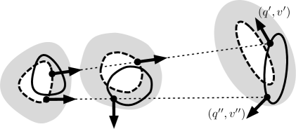
Figure 2. Action of the map $F_{\mathcal{K}^{\prime},\mathcal{K}}$. With the same conventions as in Figure 1, the point in $\mathcal{M}$ corresponding to the plane vector $(q^{\prime},v^{\prime})$ has more than one preimage, whereas the point corresponding to $(q^{\prime\prime},v^{\prime\prime})$ has no preimage at all.

2.2. Main results

First we introduce the following uniform finite-horizon condition: For $\mathfrak{t},\varphi>0$, $\varphi$ small, we say $\mathcal{K}\in{\mathbb{K}}_{0}$ has $(\mathfrak{t},\varphi)$-horizon if every directed open line segment in ${\mathbb{T}}^{2}$ of length $\mathfrak{t}$ meets a scatterer $\mathcal{B}_{i}$ of $\mathcal{K}$ at an angle $>\varphi$ (measured from its tangent line), with the segment approaching this point of contact from ${\mathbb{T}}^{2}\setminus\mathbf{B}_{i}$. Other intersection points between our line segment and $\cup_{j}\partial\mathbf{B}_{j}$ are permitted and no requirements are placed on the angles at which they meet; we require only that there be at least one intersection point meeting the condition above. Notice that this condition is not affected by the sudden appearance or disappearance of nearly tangential collisions of billiard trajectories with scatterers as the positions of the scatterers are shifted.

The space in which we will permit our time-dependent configurations to wander is defined as follows: We fix $0<\bar{\tau}^{\min}<\mathfrak{t}<\infty$ and $\varphi>0$, chosen so that the set

$${\mathbb{K}}={\mathbb{K}}(\bar{\tau}^{\min},(\mathfrak{t},\varphi))=\{\mathcal{K}\in{\mathbb{K}}_{0}:\bar{\tau}^{\min}<\tau^{\min}_{\mathcal{K}}\ {\rm and}\ \mathcal{K}\ {\rm has}\ (\mathfrak{t},\varphi){\rm-horizon}\}$$

is nonempty. Clearly, ${\mathbb{K}}$ is an open set, and its closure $\bar{{\mathbb{K}}}$ as a subset of ${({\mathbb{T}}^{2}\times{\mathbb{S}}^{1})}^{\mathfrak{s}}$ consists of those configurations whose $\tau^{\min}$ will be $\geq\bar{\tau}^{\min}$, and line segments of length $\mathfrak{t}$ with their end points added will meet scatterers with angles $\geq\varphi$. From Section 2.1, we know that there exists $\bar{\beta}=\beta(\bar{\tau}^{\min})>0$ such that $F_{\mathcal{K}^{\prime},\mathcal{K}}$ is defined for all $\mathcal{K},\mathcal{K}^{\prime}\in{\mathbb{K}}$ with $\mathbf{B}_{i}^{\prime}\subset\mathbf{B}_{i,\bar{\beta}}$ for all $i$ where $\{\mathbf{B}_{i}\}$ and $\{\mathbf{B}_{i}^{\prime}\}$ are the scatterers in $\mathcal{K}$ and $\mathcal{K}^{\prime}$ respectively. For simplicity, we will call the pair $(\mathcal{K},\mathcal{K}^{\prime})$ admissible (with respect to ${\mathbb{K}}$) if they satisfy the condition above. Clearly, if $\mathcal{K},\mathcal{K}^{\prime}\in{\mathbb{K}}$ are such that $d(\mathcal{K},\mathcal{K}^{\prime})<\varepsilon$ for small enough $\varepsilon$, then the pair is admissible. We also noted in Section 2.1 that for all admissible pairs,

$$\bar{\tau}^{\min}/2\leq\tau_{\mathcal{K}^{\prime},\mathcal{K}}\leq\mathfrak{t}\ .$$ (1)

We will denote by ${|f|}_{\gamma}$ the Hölder constant of a $\gamma$-Hölder continuous $f:\mathcal{M}\to{\mathbb{R}}$.

Our main result is

Theorem 1.

Given ${\mathbb{K}}={\mathbb{K}}(\bar{\tau}^{\min},(\mathfrak{t},\varphi))$, there exists $\varepsilon>0$ such that the following holds. Let $\mu^{1}$ and $\mu^{2}$ be probability measures on $\mathcal{M}$, with strictly positive, $\tfrac{1}{6}$-Hölder continuous densities $\rho^{1}$ and $\rho^{2}$ with respect to the measure $\cos\varphi\,\mathrm{d}r\,\mathrm{d}\varphi$. Given $\gamma>0$, there exist $0<\theta_{\gamma}<1$ and $C_{\gamma}>0$ such that

$$\left|\int_{\mathcal{M}}f\circ\mathcal{F}_{n}\,\mathrm{d}\mu^{1}-\int_{\mathcal{M}}f\circ\mathcal{F}_{n}\,\mathrm{d}\mu^{2}\right|\leq C_{\gamma}({\|f\|}_{\infty}+{|f|}_{\gamma})\theta_{\gamma}^{n},\quad n\leq N,$$

for all finite or infinite sequences $(\mathcal{K}_{n})_{n=0}^{N}\subset{\mathbb{K}}$ ($N\in{\mathbb{N}}\cup\{\infty\}$) satisfying $d(\mathcal{K}_{n-1},\mathcal{K}_{n})<\varepsilon$ for $1\leq n\leq N$, and all $\gamma$-Hölder continuous $f:\mathcal{M}\to{\mathbb{R}}$. The constant $C_{\gamma}=C_{\gamma}(\rho^{1},\rho^{2})$ depends on the densities $\rho^{i}$ through the Hölder constants of $\log\rho^{i}$, while $\theta_{\gamma}$ does not depend on the $\mu^{i}$. Both constants depend on ${\mathbb{K}}$ and $\varepsilon$.

None of the constants in the theorem depends on $N$. We have included the finite $N$ case to stress that our results do not depend on knowledge of scatterer movements in the infinite future; requiring such knowledge would be unereasonable for time-dependent systems. The notation “$(\mathcal{K}_{n})_{n=0}^{N},\ N\in{\mathbb{N}}\cup\{\infty\}$” is intended as shorthand for $\mathcal{K}_{1},\dots,\mathcal{K}_{N}$ for $N<\infty$, and $\mathcal{K}_{1},\mathcal{K}_{2},\dots$ (infinite sequence) for $N=\infty$.

Our next result is an extension of Theorem 1 to a situation where the geometries of the scatterers are also allowed to vary with time. We use $\kappa$ to denote the curvature of the scatterers, and use the convention that $\kappa>0$ corresponds to strictly convex scatterers. For $0<\bar{\kappa}^{\min}<\bar{\kappa}^{\max}<\infty$, $0<\bar{\tau}^{\min}<\mathfrak{t}<\infty,\ \varphi>0$ and $0<\Delta<\infty$, we let

$$\widetilde{\mathbb{K}}=\widetilde{\mathbb{K}}(\bar{\kappa}^{\min},\bar{\kappa}^{\max};\bar{\tau}^{\min},(\mathfrak{t},\varphi);\Delta)$$

denote the set of configurations $\mathcal{K}=\bigl{(}(\mathbf{B}_{1},o_{1}),\dots,(\mathbf{B}_{\mathfrak{s}},o_{\mathfrak{s}})\bigr{)}$ where $(\mathbf{B}_{1},\dots,\mathbf{B}_{\mathfrak{s}})$ is an ordered set of disjoint scatterers on ${\mathbb{T}}^{2}$, $o_{i}\in\partial\mathbf{B}_{i}$ is a marked point for each $i$, $\mathfrak{s}\in\mathbb{N}$ is arbitrary, and the following conditions are satisfied:

(i) the scatterer boundaries $\partial\mathbf{B}_{i}$ are $C^{3+\mathrm{Lip}}$ with $\|D(\partial\mathbf{B}_{i})\|_{C^{2}}<\Delta$ and $\mathrm{Lip}(D^{3}(\partial\mathbf{B}_{i}))<\Delta$,

(ii) the curvatures of $\partial\mathbf{B}_{i}$ lie between $\bar{\kappa}^{\min}$ and $\bar{\kappa}^{\max}$, and

(iii) $\tau_{\mathcal{K}}^{\min}>\bar{\tau}^{\min}$, and $\mathcal{K}$ has $(\mathfrak{t},\varphi)$-horizon.

In (i), $\|D(\partial\mathbf{B}_{i})\|_{C^{2}}$ and $\mathrm{Lip}(D^{3}(\partial\mathbf{B}_{i}))$ are defined to be $\max_{1\leq k\leq 3}\|D^{k}\gamma_{i}\|_{\infty}$ and $\mathrm{Lip}(D^{3}\gamma_{i})$, respectively, where $\gamma_{i}$ is the unit speed clockwise parametrization of $\mathbf{B}_{i}$. For two configurations $\mathcal{K}=((\mathbf{B}_{1},o_{1}),\dots,(\mathbf{B}_{\mathfrak{s}},o_{\mathfrak{s}}))$ and $\mathcal{K}^{\prime}=((\mathbf{B}^{\prime}_{1},o^{\prime}_{1}),\dots,(\mathbf{B}^{\prime}_{\mathfrak{s}},o^{\prime}_{\mathfrak{s}}))$ with the same number of scatterers, we define $d_{3}(\mathcal{K},\mathcal{K}^{\prime})$ to be the maximum of $\max_{i\leq\mathfrak{s}}\sup_{x\in\mathcal{M}}d_{\mathcal{M}}(\hat{\gamma}_{i}(x),\hat{\gamma}_{i}^{\prime}(x))$ and $\max_{i\leq\mathfrak{s}}\max_{1\leq k\leq 3}\|D^{k}\hat{\gamma}_{i}-D^{k}\hat{\gamma}^{\prime}_{i}\|_{\infty}$ where $\hat{\gamma}_{i}:{\mathbb{S}}^{1}\to{\mathbb{T}}^{2}$ denotes the constant speed clockwise parametrization of $\partial\mathbf{B}_{i}$ with $\hat{\gamma}_{i}(0)=o_{i}$, $\hat{\gamma}_{i}^{\prime}$ is the corresponding parametrization of $\partial\mathbf{B}^{\prime}_{i}$ with $\hat{\gamma}^{\prime}_{i}(0)=o^{\prime}_{i}$, and $d_{\mathcal{M}}$ is the natural distance on $\mathcal{M}$. The definition of admissibility for $\mathcal{K}$ and $\mathcal{K}^{\prime}$ is as above, and the billiard map $F_{\mathcal{K}^{\prime},\mathcal{K}}$ is defined as before for admissible pairs. Configurations $\mathcal{K},\mathcal{K}^{\prime}$ with different numbers of scatterers are not admissible, and the distance between them is set arbitrarily to be $d_{3}(\mathcal{K},\mathcal{K}^{\prime})=1$.

Theorem 2.

The statement of Theorem 1 holds verbatim with $({\mathbb{K}},d)$ replaced by $(\widetilde{\mathbb{K}},d_{3})$.

Theorems 1’ and 2’: The regularity assumption on the measures $\mu^{i}$ in Theorems 1–2 above can be much relaxed. It suffices to assume that the $\mu^{i}$ have regular conditional measures on unstable curves; they can be singular in the transverse direction and can, e.g., be supported on a single unstable curve. Convex combinations of such measures are also admissible. Precise conditions are given in Section 4, after we have introduced the relevant technical definitions. Theorems 1’–2’, which are the extensions of Theorems 1–2 respectively to the case where these relaxed conditions on $\mu^{i}$ are permitted, are stated in Section 4.4.

Theorems 2 and 2’ obviously apply as a special case to classical billiards, giving uniform bounds of the kind above for all $F_{\mathcal{K},\mathcal{K}}$, $\mathcal{K}\in\widetilde{\mathbb{K}}$. It is also a standard fact that correlation decay results can be deduced from the type of convergence in Theorems 1–2. To our knowledge, the following result on correlation decay for classical billiards is new. (See also pp. 149–150 in [9] for related observations.) The proof can be found in Section 8.2.

Theorem 3.

Let $\mu$ denote the measure obtained by normalizing $\cos\varphi\,\mathrm{d}r\,\mathrm{d}\varphi$ to a probability measure. Let $\widetilde{\mathbb{K}}$ be fixed, and let $\gamma>0$ be arbitrary. Then for any $\gamma$-Hölder continuous $f$ and any $\tfrac{1}{6}$-Hölder continuous $g$, there exists a constant $C^{\prime}_{\gamma}$ such that

$$\left|\int f\circ F^{n}\cdot g\,\mathrm{d}\mu-\int f\,\mathrm{d}\mu\int g\,\mathrm{d}\mu\right|\leq C_{\gamma}^{\prime}\,\theta_{\gamma}^{n}$$

hold for all $n\geq 0$ and for all $F=F_{\mathcal{K},\mathcal{K}}$ with $\mathcal{K}\in\widetilde{\mathbb{K}}$. Here $\theta_{\gamma}$ is as in the theorems above. The constant $C_{\gamma}^{\prime}$ depends on $\|f\|_{\infty}$, $|f|_{\gamma}$, $\|g\|_{\infty}$ and $|g|_{\frac{1}{6}}$.

We remark that Theorem 3 can also be formulated for sequences of maps. In that case the quantity bounded is $\int f\circ\mathcal{F}_{n}\cdot g\,\mathrm{d}\mu-\int f\circ\mathcal{F}_{n}\,\mathrm{d}\mu\,\int g\,\mathrm{d}\mu$ and $\mu$ is an arbitrary measure satisfying the conditions in Theorems 1’ and 2’. The proof is unchanged.

In addition to the broader class of measures, Theorem 2 could be extended to less regular observables $f$, which would allow for a corresponding generalization of Theorem 3. In particular, the observables could be allowed to have discontinuities at the singularities of the map $F$; see, e.g., [10]. In order to keep the focus on what is new, we do not pursue that here.

We state one further extension of the above theorems, to include the situation where the test particle is also under the influence of an external field. Given an admissible pair $(\mathcal{K},\mathcal{K}^{\prime})$ in $\widetilde{\mathbb{K}}$ and a vector field $\mathbf{E}=\mathbf{E}(\mathbf{q},\mathbf{v})$, we define first a continuous time system in which the trajectory of the test particle between collisions is determined by the equations

$$\dot{\mathbf{q}}=\mathbf{v}\quad\text{and}\quad\dot{\mathbf{v}}=\mathbf{E},$$

where $\mathbf{q}$ is the position and $\mathbf{v}$ the velocity of the particle, together with the initial condition. For the sake of simplicity, let us assume that the field is isokinetic — that is, $\mathbf{v}\cdot\mathbf{E}=0$ — which allows to normalize $|\mathbf{v}|=1$. This class of forced billiards includes “electric fields with Gaussian thermostats” studied in [14, 9] and many other papers. (Instead of the speed, more general integrals of the motion could be considered, allowing for other types of fields, such as gradients of weak potentials; see [5, 7].) Assuming that the field $\mathbf{E}$ is smooth and small, the trajectories are almost linear, and a billiard map $F^{\mathbf{E}}_{\mathcal{K}^{\prime},\mathcal{K}}:\mathcal{M}\to\mathcal{M}$ can be defined exactly as before. (See Section 8.3 for more details.) Note that $F^{\mathbf{0}}_{\mathcal{K}^{\prime},\mathcal{K}}=F_{\mathcal{K}^{\prime},\mathcal{K}}$.

The setup for our time-dependent systems result is as follows: We consider the space $\widetilde{\mathbb{K}}\times{\mathbb{E}}$ where $\widetilde{\mathbb{K}}$ is as above and ${\mathbb{E}}={\mathbb{E}}(\varepsilon^{\mathbf{E}})$ for some $\varepsilon^{\mathbf{E}}>0$ is the set of fields $\mathbf{E}\in C^{2}$ with $\|\mathbf{E}\|_{C^{2}}=\max_{0\leq k\leq 2}\|D^{k}\mathbf{E}\|_{\infty}<\varepsilon^{\mathbf{E}}$. In the theorem below, it is to be understood that $F_{n}=F^{\mathbf{E}_{n}}_{\mathcal{K}_{n},\mathcal{K}_{n-1}}$ and $\mathcal{F}_{n}=F_{n}\circ\dots\circ F_{1}$.

Theorem E. Given $\widetilde{\mathbb{K}}$, there exist $\varepsilon>0$ and $\varepsilon^{\mathbf{E}}>0$ such that the statement of Theorem 2 holds for all sequences $((\mathcal{K}_{n},\mathbf{E}_{n}))_{n\leq N}$ in $\widetilde{\mathbb{K}}\times{\mathbb{E}}(\varepsilon^{\mathbf{E}})$ satisfying $d_{3}(\mathcal{K},\mathcal{K}^{\prime})<\varepsilon$ for all $n\leq N$.

Like the zero-field case, Theorem E also admits a generalization of measures (and observables) and also implies an exponential correlation bound.

2.3. Main technical result

To prove Theorem 1, we will, in fact, prove the following technical result. All configurations below are in ${\mathbb{K}}$. Let $(\widetilde{\mathcal{K}}_{q})_{q=1}^{Q}$ ($Q\in\mathbb{Z}^{+}$ arbitrary) be a sequence of configurations, $(\tilde{\varepsilon}_{q})_{q=1}^{Q}$ a sequence of positive numbers, and $(\widetilde{N}_{q})_{q=1}^{Q}$ a sequence of positive integers. We say the configuration sequence $(\mathcal{K}_{n})_{n=0}^{N}$ (arbitrary $N$) is adapted to $(\widetilde{\mathcal{K}}_{q},\tilde{\varepsilon}_{q},\widetilde{N}_{q})_{q=1}^{Q}$ if there exist numbers $0=n_{0}<n_{1}<\dots<n_{Q}=N$ such that for $1\leq q\leq Q$, we have $n_{q}-n_{q-1}\geq\widetilde{N}_{q}$ and $\mathcal{K}_{n}\in\mathcal{N}_{\tilde{\varepsilon}_{q}}(\widetilde{\mathcal{K}}_{q})$ for $n_{q-1}\leq n\leq n_{q}$. That is to say, we think of the $(\widetilde{\mathcal{K}}_{q})_{q=1}^{Q}$ as reference configurations, and view the sequence of interest, $(\mathcal{K}_{n})_{n=0}^{N}$, as going from one reference configuration to the next, spending a long time ($\geq\widetilde{N}_{q}$) near (within $\tilde{\varepsilon}_{q}$ of) each $\widetilde{\mathcal{K}}_{q}$.

Theorem 4.

For any $\mathcal{K}\in{\mathbb{K}}$, there exist $\widetilde{N}(\mathcal{K})\geq 1$ and $\tilde{\varepsilon}(\mathcal{K})>0$ such that the following holds for every sequence of reference configurations $(\widetilde{\mathcal{K}}_{q})_{q=1}^{Q}$ ($Q<\infty$) with $\widetilde{\mathcal{K}}_{q+1}\in\mathcal{N}_{\tilde{\varepsilon}(\widetilde{\mathcal{K}}_{q})}(\widetilde{\mathcal{K}}_{q})$ for $1\leq q<Q$ and every sequence $(\mathcal{K}_{n})_{n=0}^{N}$ adapted to $(\widetilde{\mathcal{K}}_{q},\tilde{\varepsilon}(\widetilde{\mathcal{K}}_{q}),\widetilde{N}(\widetilde{\mathcal{K}}_{q}))_{q=1}^{Q}$, all configurations to be taken in ${\mathbb{K}}$: Let $\mu^{1}$ and $\mu^{2}$ be probability measures on $\mathcal{M}$, with strictly positive, $\tfrac{1}{6}$-Hölder continuous densities $\rho^{1}$ and $\rho^{2}$ with respect to the measure $\cos\varphi\,\mathrm{d}r\,\mathrm{d}\varphi$. Given any $\gamma>0$, there exist $0<\theta_{\gamma}<1$ and $C_{\gamma}>0$ such that

$$\left|\int_{\mathcal{M}}f\circ\mathcal{F}_{n}\,\mathrm{d}\mu^{1}-\int_{\mathcal{M}}f\circ\mathcal{F}_{n}\,\mathrm{d}\mu^{2}\right|\leq C_{\gamma}({\|f\|}_{\infty}+{|f|}_{\gamma})\theta_{\gamma}^{n},\qquad n\leq N,$$ (2)

for all $\gamma$-Hölder continuous $f:\mathcal{M}\to{\mathbb{R}}$. The constants $C_{\gamma}$ and $\theta_{\gamma}$ depend on the collection $\{\widetilde{\mathcal{K}}_{q},1\leq q\leq Q\}$ (see Remark 5 below); additionally $C_{\gamma}=C_{\gamma}(\rho^{1},\rho^{2})$ depends on the densities $\rho^{i}$ through the Hölder constants of $\log\rho^{i}$, while $\theta_{\gamma}$ does not depend on the $\mu^{i}$.

Remark 5.

We clarify that the constants $C_{\gamma}$ and $\theta_{\gamma}$ depend on the collection of distinct configurations that appear in the sequence $(\widetilde{\mathcal{K}}_{q})_{q=1}^{Q}$, not on the order in which these configurations are listed; in particular, each $\widetilde{\mathcal{K}}_{q}$ may appear multiple times. This observation is essential for the proofs of Theorems 1–3.

Proof of Theorem 1 assuming Theorem 4.

Given ${\mathbb{K}}$, consider a slightly larger ${\mathbb{K}}^{\prime}\supset\bar{\mathbb{K}}$, obtained by decreasing $\bar{\tau}^{\min}$ and $\varphi$ and increasing $\mathfrak{t}$. We apply Theorem  4 to ${\mathbb{K}}^{\prime}$, obtaining $\tilde{\varepsilon}(\mathcal{K})$ and $\widetilde{N}(\mathcal{K})$ for $\mathcal{K}\in{\mathbb{K}}^{\prime}$. Since $\bar{\mathbb{K}}$ is compact, there exists a finite collection of configurations $(\widetilde{\mathcal{K}}_{q})_{q\in\mathcal{Q}}\subset\bar{\mathbb{K}}$ such that the sets $\widetilde{\mathcal{N}}_{q}=\mathcal{N}_{\frac{1}{2}\tilde{\varepsilon}(\widetilde{\mathcal{K}}_{q})}(\widetilde{\mathcal{K}}_{q})\cap{\mathbb{K}}$, $q\in\mathcal{Q}$, form a cover of ${\mathbb{K}}$. Let $\varepsilon_{\star}=\min_{q\in\mathcal{Q}}\tilde{\varepsilon}(\widetilde{\mathcal{K}}_{q})$ and $N_{\star}=\max_{q\in\mathcal{Q}}\widetilde{N}(\widetilde{\mathcal{K}}_{q})$. We claim that Theorem 1 holds with $\varepsilon=\varepsilon_{\star}/(2N_{\star})$. Let $(\mathcal{K}_{n})_{n=0}^{N}\subset{\mathbb{K}}$ with $d(\mathcal{K}_{n},\mathcal{K}_{n+1})<\varepsilon$ be given. Suppose $\mathcal{K}_{0}\in\widetilde{\mathcal{N}}_{q}$. Then $\mathcal{K}_{i}$ is guaranteed to be in $\mathcal{N}_{\tilde{\varepsilon}(\widetilde{\mathcal{K}}_{q})}(\widetilde{\mathcal{K}}_{q})$ for all $i<N_{\star}$. Before the sequence leaves $\mathcal{N}_{\tilde{\varepsilon}(\widetilde{\mathcal{K}}_{q})}(\widetilde{\mathcal{K}}_{q})$, we select another $\widetilde{\mathcal{N}}_{q^{\prime}}$ and repeat the process. Thus, the assumptions of Theorem 4 are satisfied (add more copies of $\mathcal{K}_{N}$ at the end if necessary). Taking note of Remark 5, this yields a uniform rate of memory loss for all sequences. Of course the constants thus obtained for ${\mathbb{K}}$ in Theorem 1 are the constants above obtained for the larger ${\mathbb{K}}^{\prime}$ in Theorem 4. ∎

Standing Hypothesis for Sections 3–8.1: We assume ${\mathbb{K}}$ as defined by $\bar{\tau}^{\min}$, $\mathfrak{t}$ and $\varphi$ is fixed throughout. For definiteness we fix also $\bar{\beta}$, and declare once and for all that all pairs $(\mathcal{K},\mathcal{K}^{\prime})$ for which we consider the billiard map $F_{\mathcal{K}^{\prime},\mathcal{K}}$ are assumed to be admissible, as are $(\mathcal{K}_{n},\mathcal{K}_{n+1})$ in all the sequences $(\mathcal{K}_{n})$ studied. These are the only billiard maps we will consider.

3. Preliminaries I: Geometry of billiard maps

In this section, we record some basic facts about time-dependent billiard maps related to their hyperbolicity, discontinuities, etc. The results here are entirely analogous to the fixed scatterers case. They depend on certain geometric facts that are uniform for all the billiard maps considered; indeed one does not know from step to step in the proofs whether or not the source and target configurations are different. Thus we will state the facts but not give the proofs, referring the reader instead to sources where proofs are easily modified to give the results here.

An important point is that the estimates of this section are uniform, i.e., the constants in the statements of the lemmas depend only on ${\mathbb{K}}$.

Notation: Throughout the paper, the length of a smooth curve $W\subset\mathcal{M}$ is denoted by $|W|$ and the Riemannian measure induced on $W$ is denoted by $\mathfrak{m}_{W}$. Thus, $\mathfrak{m}_{W}(W)=|W|$. We denote by $\mathcal{U}_{\varepsilon}(E)$ the open $\varepsilon$-neighborhood of a set $E$ in the phase space $\mathcal{M}$. For $x=(r,\varphi)\in\mathcal{M}$, we denote by $T_{x}\mathcal{M}$ the tangent space of $\mathcal{M}$ and by $D_{x}F$ the derivative of a map $F$ at $x$. Where no ambiguity exists, we sometimes write $F$ instead of $F_{\mathcal{K}^{\prime},\mathcal{K}}$.

3.1. Hyperbolicity

Given $(\mathcal{K},\mathcal{K}^{\prime})$ and a point $x=(r,\varphi)\in\mathcal{M}$, we let $x^{\prime}=(r^{\prime},\varphi^{\prime})=Fx$ and compute $D_{x}F$ as follows: Let $\kappa(x)$ denote the curvature of $\cup_{i}\partial B_{i}$ at the point corresponding to $x$, and define $\kappa(x^{\prime})$ analogously. The flight time between $x$ and $x^{\prime}$ is denoted by $\tau(x)=\tau_{\mathcal{K}^{\prime},\mathcal{K}}(x)$. Then $D_{x}F$ is given by

$$-\frac{1}{\cos\varphi^{\prime}}\begin{pmatrix}\tau(x)\kappa(x)+\cos\varphi&\tau(x)\\ \tau(x)\kappa(x)\kappa(x^{\prime})+\kappa(x)\cos\varphi^{\prime}+\kappa(x^{\prime})\cos\varphi&\tau(x)\kappa(x^{\prime})+\cos\varphi^{\prime}\\ \end{pmatrix}$$

provided $x\notin F^{-1}\partial\mathcal{M}$, the discontinuity set of $F$. This computation is identical to the case with fixed scatterers. As in the fixed scatterers case, notice that as $x$ approaches $F^{-1}\partial\mathcal{M}$, $\cos\varphi^{\prime}\to 0$ and the derivative of the map $F$ blows up. Notice also that

$$\det D_{x}F=\cos\varphi/\cos\varphi^{\prime},$$ (3)

so that $F$ is locally invertible.

The next result asserts the uniform hyperbolicity of $F$ for orbits that do not meet $F^{-1}\partial\mathcal{M}$. Let $\kappa^{\min}$ and $\kappa^{\max}$ denote the minimum and maximum curvature of the boundaries of the scatterers $B_{i}$.

Lemma 6 (Invariant cones).

The unstable cones

$$\mathcal{C}_{x}^{u}=\{(\mathrm{d}r,\mathrm{d}\varphi)\in T_{x}\mathcal{M}\,:\,\kappa^{\min}\leq\mathrm{d}\varphi/\mathrm{d}r\leq\kappa^{\max}+2/\bar{\tau}^{\min}\},\quad x\in\mathcal{M},$$

are $D_{x}F$-invariant for all pairs $(\mathcal{K},\mathcal{K}^{\prime})$, i.e., $D_{x}F(\mathcal{C}_{x}^{u})\subset\mathcal{C}_{Fx}^{u}$ for all $x\notin F^{-1}\partial\mathcal{M}$, and there exist uniform constants $\hat{c}>0$ and $\Lambda>1$ such that for every $(\mathcal{K}_{n})_{n=0}^{N}$,

$$\|D_{x}\mathcal{F}_{n}v\|\geq\hat{c}\Lambda^{n}\|v\|$$ (4)

for all $n\in\{1,\dots,N\}$, $v\in\mathcal{C}^{u}_{x}$, and $x\notin\cup_{m=1}^{N}(\mathcal{F}_{m})^{-1}\partial\mathcal{M}$.

Similarly, the stable cones

$$\mathcal{C}_{x}^{s}=\{(\mathrm{d}r,\mathrm{d}\varphi)\in T_{x}\mathcal{M}\,:\,-\kappa^{\max}-2/\bar{\tau}^{\min}\leq\mathrm{d}\varphi/\mathrm{d}r\leq-\kappa^{\min}\}$$

are $(D_{x}F)^{-1}$-invariant for all $(\mathcal{K},\mathcal{K}^{\prime})$, i.e., $(D_{x}F)^{-1}\mathcal{C}_{Fx}^{s}\subset\mathcal{C}_{x}^{s}$ for all $x\notin\partial\mathcal{M}\cup F^{-1}\partial\mathcal{M}$, and for every $(\mathcal{K}_{n})_{n=0}^{N}$,

$$\|(D_{x}\mathcal{F}_{n})^{-1}v\|\geq\hat{c}\Lambda^{n}\|v\|$$

for all $n\in\{1,\dots,N\}$, $v\in\mathcal{C}^{s}_{\mathcal{F}_{n}x}$, and $x\notin\partial\mathcal{M}\cup\cup_{m=1}^{N}(\mathcal{F}_{m})^{-1}\partial\mathcal{M}$.

Notice that the cones here can be chosen independently of $x$ and of the scatterer configurations involved. The proof follows verbatim that of the fixed scatterers case; see [10].

Following convention, we introduce for purposes of controlling distortion (see Lemma 9) the homogeneity strips

$${\mathbb{H}}_{k} = \{(r,\varphi)\in\mathcal{M}\,:\,\pi/2-k^{-2}<\varphi\leq\pi/2-(k+1)^{-2}\}$$

$${\mathbb{H}}_{-k} = \{(r,\varphi)\in\mathcal{M}\,:\,-\pi/2+(k+1)^{-2}\leq\varphi<-\pi/2+k^{-2}\}$$

for all integers $k\geq k_{0}$, where $k_{0}$ is a sufficiently large uniform constant. It follows, for example, that for each $k$, $D_{x}F$ is uniformly bounded for $x\in F^{-1}({\mathbb{H}}_{-k}\cup{\mathbb{H}}_{k})$, as

$$C_{\mathrm{\cos}}^{-1}k^{-2}\leq\cos\varphi^{\prime}\leq C_{\mathrm{\cos}}k^{-2}$$ (5)

for a constant $C_{\mathrm{\cos}}>0$. We will also use the notation

$${\mathbb{H}}_{0}=\{(r,\varphi)\in\mathcal{M}\,:\,-\pi/2+k_{0}^{2}\leq\varphi\leq\pi/2-k_{0}^{-2}\}\ .$$

3.2. Discontinuity sets and homogeneous components

For each $(\mathcal{K},\mathcal{K}^{\prime})$, the singularity set $(F_{\mathcal{K}^{\prime},\mathcal{K}})^{-1}\partial\mathcal{M}$ has similar geometry as in the case $\mathcal{K}^{\prime}=\mathcal{K}$. In particular, it is the union of finitely many $C^{2}$-smooth curves which are negatively sloped, and there are uniform bounds depending only on ${\mathbb{K}}$ for the number of smooth segments (as follows from (1)) and their derivatives. One of the geometric facts, true for fixed scatterers as for the time-dependent case, that will be useful later is the following: Through every point in $F^{-1}\partial\mathcal{M}$, there is a continuous path in $F^{-1}\partial\mathcal{M}$ that goes monotonically in $\varphi$ from one component of $\partial\mathcal{M}$ to the other.

In our proofs it will be necessary to know that the structure of the singularity set varies in a controlled way with changing configurations. Let us denote

$$\mathcal{S}_{\mathcal{K}^{\prime},\mathcal{K}}=\partial\mathcal{M}\cup(F_{\mathcal{K}^{\prime},\mathcal{K}})^{-1}\partial\mathcal{M}.$$

If $\mathcal{K}$ and $\mathcal{K}^{\prime}$ are small perturbations of $\widetilde{\mathcal{K}}$, then $\mathcal{S}_{\mathcal{K}^{\prime},\mathcal{K}}$ is contained in a small neighborhood of $\mathcal{S}_{\widetilde{\mathcal{K}},\widetilde{\mathcal{K}}}$ (albeit the topology of $\mathcal{S}_{\mathcal{K}^{\prime},\mathcal{K}}$ may be slightly different from that of $\mathcal{S}_{\widetilde{\mathcal{K}},\widetilde{\mathcal{K}}}$). A proof of the following result, which suffices for our purposes, is given in the Appendix.

Lemma 7.

Given a configuration $\widetilde{\mathcal{K}}\in{\mathbb{K}}$ and a compact subset $E\subset\mathcal{M}\setminus\mathcal{S}_{\widetilde{\mathcal{K}},\widetilde{\mathcal{K}}}$, there exists $\delta>0$ such that the map $(x,\mathcal{K},\mathcal{K}^{\prime})\mapsto F_{\mathcal{K}^{\prime},\mathcal{K}}(x)$ is uniformly continuous on $E\times\mathcal{N}_{\delta}(\widetilde{\mathcal{K}})\times\mathcal{N}_{\delta}(\widetilde{\mathcal{K}})$.

While $F^{-1}\partial\mathcal{M}$ is the genuine discontinuity set for $F$, for purposes of distortion control one often treats the preimages of homogeneity lines as though they were discontinuity curves also. We introduce the following language: A set $E\subset\mathcal{M}$ is said to be homogeneous if it is completely contained in a connected component of one of the ${\mathbb{H}}_{k}$, $|k|\geq k_{0}$ or $k=0$. Let $E\subset\mathcal{M}$ be a homogeneous set. Then $F(E)$ may have more than one connected component. We further subdivide each connected component into maximal homogeneous subsets and call these the homogeneous components of $F(E)$. For $n\geq 2$, the homogeneous components of $\mathcal{F}_{n}(E)$ are defined inductively: Suppose $E_{n-1,i}$, $i\in I_{n-1}$, are the homogeneous components of $\mathcal{F}_{n-1}(E)$, for some index set $I_{n-1}$ which is at most countable. For each $i\in I_{n-1}$, the set $E_{n-1,i}$ is a homogeneous set, and we can thus define the homogeneous components of the single-step image $F_{n}(E_{n-1,i})$ as above. The subsets so obtained, for all $i\in I_{n-1}$, are the homogeneous components of $\mathcal{F}_{n}(E)$. Let $E_{n,i}^{-}=E\cap\mathcal{F}_{n}^{-1}(E_{n,i})$. We call ${\{E_{n,i}^{-}\}}_{i}$ the canonical $n$-step subdivision of $E$, leaving the dependence on the sequence implicit when there is no ambiguity.

For $x,y\in\mathcal{M}$, we define the separation time $s(x,y)$ to be the smallest $n\geq 0$ for which $\mathcal{F}_{n}x$ and $\mathcal{F}_{n}y$ belong in different strips ${\mathbb{H}}_{k}$ or in different connected components of $\mathcal{M}$. Observe that this definition is $(\mathcal{K}_{n})$-dependent.

3.3. Unstable curves

A connected $C^{2}$-smooth curve $W\subset\mathcal{M}$ is called an unstable curve if $T_{x}W\subset\mathcal{C}^{u}_{x}$ for every $x\in W$. It follows from the invariant cones condition that the image of an unstable curve under $\mathcal{F}_{n}$ is a union of unstable curves. Our unstable curves will be parametrized by $r$: for a curve $W$, we write $\varphi=\varphi_{W}(r)$.

For an unstable curve $W$, define $\hat{\kappa}_{W}=\sup_{W}|\mathrm{d}^{2}\varphi_{W}/\mathrm{d}r^{2}|$.

Lemma 8.

There exist uniform constants $C_{\mathrm{c}}>0$ and $\vartheta_{\mathrm{c}}\in(0,1)$ such that the following holds. Let $W$ and $\mathcal{F}_{n}W$ be unstable curves. Then

$$\hat{\kappa}_{\mathcal{F}_{n}W}\leq\frac{C_{\mathrm{c}}}{2}(1+\vartheta_{\mathrm{c}}^{n}\hat{\kappa}_{W}).$$

We call an unstable curve $W$ regular if it is homogeneous and satisfies the curvature bound $\hat{\kappa}_{W}\leq C_{c}$. Thus for any unstable curve $W$, all homogeneous components of $\mathcal{F}_{n}(W)$ are regular for large enough $n$.

Given a smooth curve $W\subset\mathcal{M}$, define

$$\mathcal{J}_{W}\mathcal{F}_{n}(x)={\|D_{x}\mathcal{F}_{n}v\|}/{\|v\|}$$

for any nonzero vector $v\in T_{x}W$. In other words, $\mathcal{J}_{W}\mathcal{F}_{n}$ is the Jacobian of the restriction $\mathcal{F}_{n}|_{W}$.

Lemma 9 (Distortion bound).

There exist uniform constants $C_{\mathrm{d}}^{\prime}>0$ and $C_{\mathrm{d}}>0$ such that the following holds. Given $(\mathcal{K}_{n})_{n=0}^{N}$, if $\mathcal{F}_{n}W$ is a homogeneous unstable curve for $0\leq n\leq N$, then

$$C_{\mathrm{d}}^{-1}\leq e^{-C_{\mathrm{d}}^{\prime}|\mathcal{F}_{n}W|^{1/3}}\leq\frac{\mathcal{J}_{W}\mathcal{F}_{n}(x)}{\mathcal{J}_{W}\mathcal{F}_{n}(y)}\leq e^{C_{\mathrm{d}}^{\prime}|\mathcal{F}_{n}W|^{1/3}}\leq C_{\mathrm{d}}$$ (6)

for every pair $x,y\in W$ and $0\leq n\leq N$.

Finally, we state a result which asserts that very short homogeneous curves cannot acquire lengths of order one arbitrarily fast, in spite of the fact that the local expansion factor is unbounded.

Lemma 10.

There exists a uniform constant $C_{\mathrm{e}}\geq 1$ such that

$$|\mathcal{F}_{n}W|\leq C_{\mathrm{e}}|W|^{1/2^{n}},$$

if $W$ is an unstable curve and $\mathcal{F}_{m}W$ is homogeneous for $0\leq m<n$.

The proofs of these results also follow closely those for the fixed scatterers case. For Lemma 8, see [8]. For Lemmas 9 and 10, see [10]. (Lemma  10 follows readily by iterating the corresponding one-step bound.)

3.4. Local stable manifolds

Given $(\mathcal{K}_{n})_{n\geq 0}$, a connected smooth curve $W$ is called a homogeneous local stable manifold, or simply local stable manifold, if the following hold for every $n\geq 0$:

(i) $\mathcal{F}_{n}W$ is connected and homogeneous, and

(ii) $T_{x}(\mathcal{F}_{n}W)\subset\mathcal{C}^{s}_{x}$ for every $x\in\mathcal{F}_{n}W$.

It follows from Lemma 6 that local stable manifolds are exponentially contracted under $\mathcal{F}_{n}$. We stress that unlike unstable curves, the definition of local stable manifolds depends strongly on the infinite sequence of billiard maps defined by $(\mathcal{K}_{n})_{n\geq 0}$.

For $x\in\mathcal{M}$, let $W^{s}(x)$ denote the maximal local stable manifold through $x$ if one exists. An important result is the absolute continuity of local stable manifolds. Let two unstable curves $W^{1}$ and $W^{2}$ be given. Denote $W^{i}_{\star}=\{x\in W^{i}\,:\,W^{s}(x)\cap W^{3-i}\neq 0\}$ for $i=1,2$. The map ${\mathbf{h}}:W^{1}_{\star}\to W^{2}_{\star}$ such that $\{{\mathbf{h}}(x)\}=W^{s}(x)\cap W^{2}$ for every $x\in W^{1}_{\star}$ is called the holonomy map. The Jacobian $\mathcal{J}{\mathbf{h}}$ of the holonomy is the Radon–Nikodym derivative of the pullback ${\mathbf{h}}^{-1}(\mathfrak{m}_{W^{2}}|_{W^{2}_{*}})$ with respect to $\mathfrak{m}_{W^{1}}$. The following result gives a uniform bound on the Jacobian almost everywhere on $W^{1}_{\star}$.

Lemma 11.

Let $W^{1}$ and $W^{2}$ be regular unstable curves. Suppose ${\mathbf{h}}:W^{1}_{\star}\to W^{2}_{\star}$ is defined on a positive $\mathfrak{m}_{W^{1}}$-measure set $W^{1}_{\star}\subset W^{1}$. Then for $\mathfrak{m}_{W^{1}}$-almost every point $x\in W^{1}_{\star}$,

$$\mathcal{J}{\mathbf{h}}(x)=\lim_{n\to\infty}\frac{\mathcal{J}_{W^{1}}\mathcal{F}_{n}(x)}{\mathcal{J}_{W^{2}}\mathcal{F}_{n}({\mathbf{h}}(x))},$$ (7)

where the limit exists and is positive with uniform bounds. In fact, there exist uniform constants $A_{\mathbf{h}}>0$ and $C_{\mathbf{h}}>0$ such that the following holds: If $\alpha(x)$ denotes the difference between the slope of the tangent vector of $W^{1}$ at $x$ and that of $W^{2}$ at ${\mathbf{h}}(x)$, and if $\delta(x)$ is the distance between $x$ and ${\mathbf{h}}(x)$, then

$$A_{\mathbf{h}}^{-\alpha-\delta^{1/3}}\leq\mathcal{J}{\mathbf{h}}\leq A_{\mathbf{h}}^{\alpha+\delta^{1/3}}$$ (8)

almost everywhere on $W^{1}_{\star}$. Moreover, with $\theta=\Lambda^{-1/6}\in(0,1)$,

$$|\mathcal{J}{\mathbf{h}}(x)-\mathcal{J}{\mathbf{h}}(y)|\leq C_{\mathbf{h}}\theta^{s(x,y)}$$ (9)

holds for all pairs $(x,y)$ in $W^{1}_{\star}$, where $s(x,y)$ is the separation time defined in Section 3.2.

The proof of Lemma 11 follows closely its counterpart for fixed configurations. The identity in (7) is standard for uniformly hyperbolic systems (see [1, 17]), as is (9), except for the use of separation time as a measure of distance in discontinuous systems; see [20, 10].

4. Preliminaries II: Evolution of measured unstable curves

4.1. Growth of unstable curves

Given a sequence $(\mathcal{K}_{m})$, an unstable curve $W$, a point $x\in W$, and an integer $n\geq 0$, we denote by $r_{W,n}(x)$ the distance between $\mathcal{F}_{n}x$ and the boundary of the homogeneous component of $\mathcal{F}_{n}W$ containing $\mathcal{F}_{n}x$.

The following result, known as the Growth lemma, is key in the analysis of billiard dynamics. It expresses the fact that the expansion of unstable curves dominates the cutting by $\partial\mathcal{M}\cup\cup_{|k|\geq k_{0}}\partial{\mathbb{H}}_{k}$, in a uniform fashion for all sequences. The reason behind this fact is that unstable curves expand at a uniform exponential rate, whereas the cuts accumulate at tangential collisions. A short unstable curve can meet no more than $\mathfrak{t}/\bar{\tau}^{\min}$ tangencies in a single time step (see (1)), so the number of encountered tangencies grows polynomially with time until a characteristic length has been reached. The proof follows verbatim that in the fixed configuration case; see [10].

Lemma 12 (Growth lemma).

There exist uniform constants $C_{\mathrm{gr}}>0$ and $\vartheta\in(0,1)$ such that, for all (finite or infinite) sequences $(\mathcal{K}_{n})_{n=0}^{N}$, unstable curves $W$ and $0\leq n\leq N$:

$$\mathfrak{m}_{W}\{r_{W,n}<\varepsilon\}\leq C_{\mathrm{gr}}(\vartheta^{n}+|W|)\varepsilon\ .$$

This lemma has the following interpretation: It gives no information for small $n$ when $|W|$ is small. For $n$ large enough, such as $n\geq|\log|W||/|\log\vartheta|$, one has $\mathfrak{m}_{W}\{r_{W,n}<\varepsilon\}\leq 2C_{\mathrm{gr}}\varepsilon|W|$. In other words, after a sufficiently long time $n$ (depending on the initial curve $W$), the majority of points in $W$ have their images in homogeneous components of $\mathcal{F}_{n}W$ that are longer than $1/(2C_{\mathrm{gr}})$, and the family of points belonging to shorter ones has a linearly decreasing tail.

4.2. Measured unstable curves

A measured unstable curve is a pair $(W,\nu)$ where $W$ is an unstable curve and $\nu$ is a finite Borel measure supported on it. Given a sequence $(\mathcal{K}_{n})_{n=0}^{\infty}$ and a measured unstable curve $(W,\nu)$ with density $\rho=\mathrm{d}\nu/\mathrm{d}\mathfrak{m}_{W}$, we are interested in the following dynamical Hölder condition of $\log\rho$: For $n\geq 1$, let ${\{W_{n,i}^{-}\}}_{i}$ be the canonical $n$-step subdivision of $W$ as defined in Section 3.2.

Lemma 13.

There exists a constant $C^{\prime}_{\mathrm{r}}>0$ for which the following holds: Suppose $\rho$ is a density on an unstable curve $W$ satisfying $|\log\rho(x)-\log\rho(y)|\leq C\theta^{s(x,y)}$ for all $x,y\in W$. Then, for any homogeneous component $W_{n,i}$, the density $\rho_{n,i}$ of the push-forward of $\nu|_{W_{n,i}}$ by the (invertible) map $\mathcal{F}_{n}|_{W_{n,i}^{-}}$ satisfies

$$|\log\rho_{n,i}(x)-\log\rho_{n,i}(y)|\leq\left(\frac{C^{\prime}_{\mathrm{r}}}{2}+\Bigl{(}C-\frac{C^{\prime}_{\mathrm{r}}}{2}\Bigr{)}\theta^{n}\!\right)\!\theta^{s(x,y)}$$ (10)

for all $x,y\in W_{n,i}$.

Here $\theta$ is as in Lemma 11. We fix $C_{\mathrm{r}}\geq\max\{C^{\prime}_{\mathrm{r}},C_{\mathbf{h}},2\}$, where $C_{\mathbf{h}}$ is also introduced in Lemma 11, and say a measure $\nu$ supported on an unstable curve $W$ is regular if it is absolutely continuous with respect to $\mathfrak{m}_{W}$ and its density $\rho$ satisfies

$$|\log\rho(x)-\log\rho(y)|\leq C_{\mathrm{r}}\theta^{s(x,y)}$$ (11)

for all $x,y\in W$. As with $s(\cdot,\cdot)$, the regularity of $\nu$ is $(\mathcal{K}_{n})$-dependent. Notice that under this definition, if a measure on $W$ is regular, then so are its forward images. More precisely, in the notation of Lemma 13, if $\rho$ is regular, then so is each $\rho_{n,i}$. We also say the pair $(W,\nu)$ is regular if both the unstable curve $W$ and the measure $\nu$ are regular.

Remark 14.

The separation time $s(x,y)$ is connected to the Euclidean distance $d_{\mathcal{M}}(x,y)$ in the following way. If $x$ and $y$ are connected by an unstable curve $W$, then $|\mathcal{F}_{n}W|\geq\hat{c}\Lambda^{n}|W|\geq\hat{c}\Lambda^{n}d_{\mathcal{M}}(x,y)$ for $0\leq n<s(x,y)$. Since $\mathcal{F}_{s(x,y)-1}W$ is a homogeneous unstable curve, its length is uniformly bounded above. Thus,

$$d_{\mathcal{M}}(x,y)\leq C_{\mathrm{s}}\Lambda^{-s(x,y)}=C_{\mathrm{s}}\theta^{6s(x,y)}$$ (12)

for a uniform constant $C_{\mathrm{s}}>0$. In particular, if $\rho$ is a nonnegative density on an unstable curve $W$ such that $\log\rho$ is Hölder continuous with exponent $1/6$ and constant $C_{\mathrm{r}}C_{\mathrm{s}}^{-1/6}$, then $\rho$ is regular with respect to any configuration sequence.

Proof of Lemma 13.

Consider $n=1$ and take two points $x,y$ on one of the homogeneous components $W_{1,i}$. Let the corresponding preimages be $x_{-1},y_{-1}$. Since $s(x_{-1},y_{-1})=s(x,y)+1$, the bound (6) yields

$$\begin{split}|\log\rho_{1,i}(x)-\log\rho_{1,i}(y)|&\leq\left|\log\frac{\rho(x_{-1})}{\mathcal{J}_{W}F_{1}(x_{-1})}-\log\frac{\rho(y_{-1})}{\mathcal{J}_{W}F_{1}(y_{-1})}\right|\\ &\leq|\log\rho(x_{-1})-\log\rho(y_{-1})|+|\log\mathcal{J}_{W}F_{1}(x_{-1})-\log\mathcal{J}_{W}F_{1}(y_{-1})|\\ &\leq C\theta^{s(x,y)+1}+C_{\mathrm{d}}^{\prime}|W_{1,i}(x,y)|^{1/3},\end{split}$$

where $|W_{1,i}(x,y)|$ is the length of the segment of the unstable curve $W_{1,i}$ connecting $x$ and $y$. Because of the unstable cones, the latter is uniformly proportional to the distance $d_{\mathcal{M}}(x,y)$ of $x$ and $y$. Recalling (12), we thus get $C_{\mathrm{d}}^{\prime}|W_{1,i}(x,y)|^{1/3}\leq C_{\mathrm{d}}^{\prime\prime}\theta^{2s(x,y)}\leq C_{\mathrm{d}}^{\prime\prime}\theta^{s(x,y)}$ for another uniform constant $C_{\mathrm{d}}^{\prime\prime}>0$. Let us now pick any $C_{\mathrm{r}}$ such that $C_{\mathrm{r}}\geq 2C_{\mathrm{d}}^{\prime\prime}/(1-\theta)$. For then $C_{\mathrm{r}}\theta+C_{\mathrm{d}}^{\prime\prime}\leq\frac{1+\theta}{2}C_{\mathrm{r}}$, and we have $|\log\rho_{1,i}(x)-\log\rho_{1,i}(y)|\leq C^{\prime}\theta^{s(x,y)}$ with

$$C^{\prime}\leq C\theta+C_{\mathrm{d}}^{\prime\prime}=(C-C_{\mathrm{r}})\theta+(C_{\mathrm{r}}\theta+C_{\mathrm{d}}^{\prime\prime})\leq(C-C_{\mathrm{r}})\theta+\frac{1+\theta}{2}C_{\mathrm{r}}=C\theta+\frac{1-\theta}{2}C_{\mathrm{r}}.$$ (13)

We may iterate (13) inductively, observing that at each step the constant $C$ obtained at the previous step is contracted by a factor of $\theta$ towards $\frac{1-\theta}{2}C_{\mathrm{r}}$. It is now a simple task to obtain (10). The constant $C_{\mathrm{r}}$ was chosen so that the image of a regular density is regular and the image of a non-regular density will become regular in finitely many steps. ∎

The following extension property of (11) will be necessary. We give a proof in the Appendix.

Lemma 15.

Suppose $W_{\star}$ is a closed subset of an unstable curve $W$, and that $W_{\star}$ includes the endpoints of $W$. Assume that the function $\rho$ is defined on $W_{\star}$ and that there exists a constant $C>0$ such that $|\log\rho(x)-\log\rho(y)|\leq C\theta^{s(x,y)}$ for every pair $(x,y)$ in $W_{\star}$. Then, $\rho$ can be extended to all of $W$ in such a way that the inequality involving $\log\rho$ above holds on $W$, the extension is piecewise constant, $\min_{W}\rho=\min_{W_{\star}}\rho$, and $\max_{W}\rho=\max_{W_{\star}}\rho$.

4.3. Families of measured unstable curves

Here we extend the idea of measured unstable curves to measured families of unstable stacks. We begin with the following definitions:

(i) We call $\cup_{\alpha\in E}W_{\alpha}\subset\mathcal{M}$ a stack of unstable curves, or simply an unstable stack, if $E\subset{\mathbb{R}}$ is an open interval, each $W_{\alpha}$ is an unstable curve, and there is a map $\psi:[0,1]\times E\to\mathcal{M}$ which is a homeomorphism onto its image so that, for each $\alpha\in E$, $\psi\bigl{(}[0,1]\times\{\alpha\}\bigr{)}=W_{\alpha}$.

(ii) The unstable stack $\cup_{\alpha\in E}W_{\alpha}$ is said to be regular if each $W_{\alpha}$ is regular as an unstable curve.

(iii) We call $(\cup_{\alpha\in E}W_{\alpha},\mu)$ a measured unstable stack if $U=\cup_{\alpha\in E}W_{\alpha}$ is an unstable stack and $\mu$ is a finite Borel measure on $U$.

(iv) we say $(\cup_{\alpha\in E}W_{\alpha},\mu)$ is regular if (a) as a stack $\cup_{\alpha\in E}W_{\alpha}$ is regular and (b) the conditional probability measures $\mu_{\alpha}$ of $\mu$ on $W_{\alpha}$ are regular. More precisely, $\{W_{\alpha},\alpha\in E\}$ is a measurable partition of $\cup_{\alpha\in E}W_{\alpha}$, and $\{\mu_{\alpha}\}$ is a version of the disintegration of $\mu$ with respect to this partition, that is to say, for any Borel set $B\subset\mathcal{M}$, we have

$$\mu(B)=\int_{E}\mu_{\alpha}(W_{\alpha}\cap B)\,\mathrm{d}P(\alpha)$$

where $P$ is a finite Borel measure on $I$. The conditional measures $\{\mu_{\alpha}\}$ are unique up to a set of $P$-measure $0$, and (b) requires that $(W_{\alpha},\mu_{\alpha})$ be regular in the sense of Section 4.2 for $P$-a.e. $\alpha$.

Consider next a sequence $(\mathcal{K}_{n})_{n=0}^{\infty}$ and a fixed $n\geq 1$. Denote by $\mathcal{D}_{n,i}$, $i\geq 1$, the countably many connected components of the set $\mathcal{M}\setminus\cup_{1\leq m\leq n}(\mathcal{F}_{m})^{-1}(\partial\mathcal{M}\cup\cup_{|k|\geq k_{0}}\partial{\mathbb{H}}_{k})$. In analogy with unstable curves, we define the canonical $n$-step subdivision of a regular unstable stack $\cup_{\alpha}W_{\alpha}$: Let $(n,i)$ be such that $\cup_{\alpha}W_{\alpha}\cap\mathcal{D}_{n,i}\neq\emptyset$, and let $E_{n,i}=\{\alpha\in E:W_{\alpha}\cap\mathcal{D}_{n,i}\neq\emptyset\}$. Pick one of the (finitely our countably many) components $E_{n,i,j}$ of $E_{n,i}$.

We claim $\cup_{\alpha\in E_{n,i,j}}(W_{\alpha}\cap\overline{\mathcal{D}}_{n,i})$ is an unstable stack, and define

$$\psi_{n,i,j}:[0,1]\times E_{n,i,j}\ \to\ \cup_{\alpha\in E_{n,i,j}}W_{\alpha}\cap\overline{\mathcal{D}}_{n,i}$$

as follows: for $\alpha\in E_{n,i}$, $\psi_{n,i}|_{[0,1]\times\{\alpha\}}$ is equal to $\psi|_{[0,1]\times\{\alpha\}}$ followed by a linear contraction from $W_{\alpha}$ to $W_{\alpha}\cap\overline{\mathcal{D}}_{n,i}$. For this construction to work, it is imperative that $W_{\alpha}\cap\mathcal{D}_{n,i}$ be connected, and that is true, for by definition, $W_{\alpha}\cap\mathcal{D}_{n,i}$ is an element of the canonical $n$-step subdivision of $W_{\alpha}$. It is also clear that $\cup_{\alpha\in E_{n,i,j}}\mathcal{F}_{n}(W_{\alpha}\cap\overline{\mathcal{D}}_{n,i})$ is an unstable stack, with the defining homeomorphism given by $\mathcal{F}_{n}\circ\psi_{n,i,j}$.

What we have argued in the last paragraph is that the $\mathcal{F}_{n}$-image of an unstable stack $\cup_{\alpha}W_{\alpha}$ is the union of at most countably many unstable stacks. Similarly, the $\mathcal{F}_{n}$-image of a measured unstable stack is the union of measured unstable stacks, and by Lemmas 8 and 13, regular measured unstable stacks are mapped to unions of regular measured unstable stacks.

Figure 3. A schematic illustration of an unstable stack and its dynamics. The regular unstable curves on the right are the images of the horizontal lines under the homeomorphism $\psi$. The curves with negative slopes represent the countably many branches of the $n$-step singularity set $\cup_{1\leq m\leq n}(\mathcal{F}_{m})^{-1}(\partial\mathcal{M}\cup\cup_{|k|\geq k_{0}}\partial{\mathbb{H}}_{k})$. The canonical $n$-step subdivision of the unstable curves yields countably many unstable stacks.

The discussion above motivates the definition of measured unstable families, defined to be convex combinations of measured unstable stacks. That is to say, we have a countable collection of unstable stacks $\cup_{\alpha\in E_{j}}W^{(j)}_{\alpha}$ parametrized by $j$, and a measure $\mu=\sum_{j}a^{(j)}\mu^{(j)}$ with the property that for each $j$, $(\cup_{\alpha}W^{(j)}_{\alpha},\mu^{(j)})$ is a measured unstable stack and $\sum_{j}a^{(j)}=1$. We permit the stacks to overlap, i.e., for $j\neq j^{\prime}$, we permit $\cup_{\alpha}W^{(j)}_{\alpha}$ and $\cup_{\alpha}W^{(j^{\prime})}_{\alpha}$ to meet. This is natural because in the case of moving scatterers, the maps $\mathcal{F}_{n}$ are not one-to-one; even if two stacks have disjoint supports, this property is not retained by the forward images. Regularity for measured unstable families is defined similarly. The idea of canonical $n$-step subdivision passes easily to measured unstable families, and we can sum up the discussion by saying that given $(\mathcal{K}_{n})$, push-forwards of measured unstable families are again measured unstable families, and regularity is preserved.

So far, we have not discussed the lengths of the unstable curves in an unstable stack or family. Following [10], we introduce, for a measured unstable family defined by $(\cup_{\alpha}W^{(j)}_{\alpha},\mu^{(j)})$ and $\mu=\sum_{j}a^{(j)}\mu^{(j)}$, the quantity

$$\mathcal{Z}=\sum_{j}a^{(j)}\int_{{\mathbb{R}}}\frac{1}{|W^{(j)}_{\alpha}|}\,\mathrm{d}P^{(j)}(\alpha).$$ (14)

Informally, the smaller the value of $\mathcal{Z}/\mu(\mathcal{M})$ the smaller the fraction of $\mu$ supported on short unstable curves.

For $\mu$ as above, let $\mathcal{Z}_{n}$ denote the quantity corresponding to $\mathcal{Z}$ for the push-forward $\sum_{k}a_{n,k}\,\mu_{n,k}$ of the canonical $n$-step subdivision of $\mu$ discussed earlier. We have the following control on $\mathcal{Z}_{n}$:

Lemma 16.

There exist uniform constants $C_{\mathrm{p}}>1$ and $\vartheta_{\mathrm{p}}\in(0,1)$ such that

$$\frac{\mathcal{Z}_{n}}{\mu(\mathcal{M})}\leq\frac{C_{\mathrm{p}}}{2}\!\left(1+\vartheta_{\mathrm{p}}^{n}\frac{\mathcal{Z}}{\mu(\mathcal{M})}\right)$$ (15)

holds true for any regular measured unstable family.

This result can be interpreted as saying that given an initial measure $\mu$ which has a high fraction of its mass supported on short unstable curves — yielding a large value of $\mathcal{Z}/\mu(\mathcal{M})$ — the mass gets quickly redistributed by the dynamics to the longer homogeneous components of the image measures, so that $\mathcal{Z}_{n}/\mu(\mathcal{M})$ decreases exponentially, until a level safely below $C_{\mathrm{p}}$ is reached. As regular densities remain regular (Lemma 13), and as the supremum and the infimum of a regular density are uniformly proportional, Lemma 16 is a direct consequence of the Growth lemma; see above. See [10] for the fixed configuration case; the time-dependent case is analogous.

Definition 17.

A regular measured unstable family is called proper if $\mathcal{Z}<C_{\mathrm{p}}\mu(\mathcal{M})$.

Notice that $\mathcal{Z}<C_{\mathrm{p}}\mu(\mathcal{M})$ implies, by Markov’s inequality and $\sum_{j}a^{(j)}P^{(j)}({\mathbb{R}})=\mu(\mathcal{M})$, that

$$\sum_{j}a^{(j)}P^{(j)}\!\left\{\alpha\in{\mathbb{R}}\,:\,|W^{(j)}_{\alpha}|\geq(2C_{\mathrm{p}})^{-1}\right\}\geq\tfrac{1}{2}\mu(\mathcal{M}).$$ (16)

In other words, if $\mu$ is proper, then at least half of it is supported on unstable curves of length $\geq(2C_{\mathrm{p}})^{-1}$. Notice also that for any measured unstable family with $\mathcal{Z}<\infty$, Lemma 16 shows that the push-forward of such a family will eventually become proper. Starting from a proper family, it is possible that $\mathcal{Z}_{n}\geq C_{\mathrm{p}}\mu(\mathcal{M})$ for a finite number of steps; however, (15) implies that there exists a uniform constant $n_{\mathrm{p}}$ such that $\mathcal{Z}_{n}<C_{\mathrm{p}}\mu(\mathcal{M})$ for all $n\geq n_{\mathrm{p}}$.

Remark 18.

The results of Sections 4.1–4.3 can be summarized as follows:

(i) The $\mathcal{F}_{n}$-image of an unstable stack is the union of at most countably many such stacks.

(ii) Regular measured unstable stacks are mapped to unions of the same, and

(iii) the $\mathcal{F}_{n}$-image of a proper measured unstable family is proper for $n\geq n_{p}$.

4.4. Statements of Theorems 1’–2’ and 4’

We are finally ready to give a precise statement of Theorem 1’, which permits more general initial distributions than Theorem 1 as stated in Section 2.2.

Theorem 1’.  There exists $\varepsilon>0$ such that the following holds. Let $(\cup_{\alpha}W^{i}_{\alpha},\mu^{i})$, $i=1,2$, be measured unstable stacks. Assume $\mathcal{Z}^{i}<\infty$ and that the conditional densities satisfy $|\log\rho^{i}_{\alpha}(x)-\log\rho^{i}_{\alpha}(y)|\leq C^{i}\theta^{s(x,y)}$ for all $x,y\in W^{i}_{\alpha}$. Given $\gamma>0$, there exist $0<\theta_{\gamma}<1$ and $C_{\gamma}>0$ such that

$$\left|\int_{\mathcal{M}}f\circ\mathcal{F}_{n}\,\mathrm{d}\mu^{1}-\int_{\mathcal{M}}f\circ\mathcal{F}_{n}\,\mathrm{d}\mu^{2}\right|\leq C_{\gamma}({\|f\|}_{\infty}+{|f|}_{\gamma})\theta_{\gamma}^{n},\quad n\leq N,$$

for all sequences $(\mathcal{K}_{n})_{n=0}^{N}\subset{\mathbb{K}}$ ($N\in{\mathbb{N}}\cup\{\infty\}$) satisfying $d(\mathcal{K}_{n-1},\mathcal{K}_{n})<\varepsilon$ for $1\leq n\leq N$, and all $\gamma$-Hölder continuous $f:\mathcal{M}\to{\mathbb{R}}$. The constant $C_{\gamma}$ depends on $\max(C^{1},C^{2})$ and $\max(\mathcal{Z}^{1},\mathcal{Z}^{2})$, while $\theta_{\gamma}$ does not.

Let us say a finite Borel measure $\mu$ is regular on unstable curves if it admits a representation as the measure in a regular measured unstable family with $\mathcal{Z}<\infty$, proper if additionally it admits a representation that is proper. It follows from Lemmas 13 and 16 that in Theorem 1’, after a finite number of steps depending on $C^{i}$ and $\mathcal{Z}^{i}$, the pushforward of $\mu^{i}$ will become regular on unstable curves and proper.

For completeness, we provide a proof of the following in the Appendix.

Lemma 19.

Theorem 1’ generalizes Theorem 1.

Theorem 2’. This is obtained from Theorems 2 in exactly the same way as Theorem 1’ is obtained from Theorem 1, namely by relaxing the condition on $\mu^{i}$ as stated.

As a matter of fact, instead of just Theorem 4, the following generalization is proved in Section 8.1.

Theorem 4’. This is a similar extension of Theorem 4, i.e., of the local result, to initial measures as stated in Theorem 1’.

We finish by remarking on our use of measured unstable stacks and families: The primary reason for considering these objects is that in the proof we really work with measured unstable curves and their images under $\mathcal{F}_{n}$. “Thin enough” stacks of unstable curves behave in a way very similar to unstable curves, and are treated similarly. Other generalizations are made so we can include a larger class of initial distributions; moreover, to the extent that is possible, it is always convenient to work with a class of objects closed under the operations of interest. See Remark 18. We note also that our formulation here has deviated from [10] because of (fixable) measurability issues with their formulation.

In view of the fact that our proof really focuses on curves, we will, for pedagogical reasons consider separately the following two cases:

• The countable case, in which we assume that each initial distribution $\mu^{i}$ is supported on a countable family of unstable curves, i.e., the stacks above consist of single curves.

• The continuous case, where we allow the $\mu^{i}$ to be as in Theorem 1’.

For clarity of exposition, we first focus on the countable case, presenting a synopsis of the proof followed by a complete proof; this is carried out in Sections 5–7. Extensions to the continuous case is discussed in Section 8.

5. Theorem 4: synopsis of proof

This important section contains a sketch of the proof, from beginning to end, of the “countable case” of Theorem 4; it will serve as a guide to the supporting technical estimates in the sections to follow. We have divided the discussion into four parts: Paragraph A contains an overview of the coupling argument on which the proof is based. The coupling procedure itself follows closely [10]; it is reviewed in Paragraphs B and C. Having an outline of the proof in hand permits us to isolate the issues directly related to the time-dependent setting; this is discussed in Paragraph D. As mentioned in the Introduction, one of the goals of this paper is to stress the (strong) similarities between stationary dynamics and their time-dependent counterparts, and to highlight at the same time the new issues that need to be addressed.

For simplicity of notation, we will limit the discussion here to the “countable case” of Theorem 4. That is to say, we assume throughout that the initial distributions $\mu^{i},i=1,2$, are proper measures supported on a countable number of unstable curves; see Section 4.3.

A. Overview of coupling argument

The following scheme is used to produce the exponential bound in Theorem 4. Let $(\mathcal{K}_{n}),n\leq N\leq\infty$ be an admissible (finite or infinite) sequence of configurations with associated composed maps $\mathcal{F}_{n}=F_{n}\circ\dots\circ F_{1}$. Given initial probability distributions $\mu^{1}$ and $\mu^{2}$ on $\mathcal{M}$, we will produce two sequences of nonnegative measures $\bar{\mu}^{i}_{n},\ n\leq N$, with properties (i)–(iii) below:

• for $i=1,2$, $\mu^{i}=\sum_{j\leq n}\bar{\mu}^{i}_{j}+\mu^{i}_{n}$ with $\bar{\mu}^{1}_{n}(\mathcal{M})=\bar{\mu}^{2}_{n}(\mathcal{M})$ for each $n$;

• $\mu^{1}_{n}(\mathcal{M})=\mu^{2}_{n}(\mathcal{M})\leq Ce^{-an}$;

• $|\int f\circ\mathcal{F}_{n+m}\,\mathrm{d}\bar{\mu}^{1}_{n}-\int f\circ\mathcal{F}_{n+m}\,\mathrm{d}\bar{\mu}^{2}_{n}|\leq C_{f}e^{-am}\bar{\mu}^{i}_{n}(\mathcal{M})$, for any test function $f$.

Here $\bar{\mu}^{i}_{n},i=1,2$, are the components of $\mu^{i}$ coupled at time $n$; their relationship from time $n$ on is given by (iii). By (ii), the yet-to-be-coupled part decays exponentially. In practice, a coupling occurs at a sequence of times $0<t_{1}<t_{2}<\cdots<t_{K}<N$. In particular, $\bar{\mu}^{i}_{j}=0$, when $j\neq t_{k}$ for all $1\leq k\leq K$, which means that $\mu_{n}^{i}$ remains unchanged between successive coupling times.

It follows from (i)–(iii) above that

$$\begin{split}\left|\int f\circ\mathcal{F}_{n}\,\mathrm{d}\mu^{1}-\int f\circ\mathcal{F}_{n}\,\mathrm{d}\mu^{2}\right|&\leq 2\|f\|_{\infty}\cdot\mu^{i}_{n/2}(\mathcal{M})+\sum_{j\leq n/2}C_{f}e^{-a(n-j)}\bar{\mu}^{i}_{j}(\mathcal{M})\ \\ &\leq 2\|f\|_{\infty}Ce^{-an/2}+C_{f}e^{-an/2}.\end{split}$$ (17)

We indicate briefly below how, at time $n$ where $n=t_{k}$ is a coupling time, we extract $\bar{\mu}^{i}_{n}$ from $\mu^{i}_{n-1}$ and couple $\bar{\mu}^{1}_{n}$ to $\bar{\mu}^{2}_{n}$. Recall that in the hypotheses of Theorem 4, $(\mathcal{K}_{m})_{m=0}^{N}$ is adapted to $(\widetilde{\mathcal{K}}_{q},\tilde{\varepsilon}(\widetilde{\mathcal{K}}_{q}),\widetilde{N}(\widetilde{\mathcal{K}}_{q}))_{q=1}^{Q}$. We assume $\mathcal{K}_{n}\in\mathcal{N}_{\tilde{\varepsilon}(\widetilde{\mathcal{K}}_{q})}(\widetilde{\mathcal{K}}_{q})$ for some $q$. In fact, coupling times are chosen so that $\mathcal{K}_{m}$ is in the same neighborhood for a large number of $m\leq n$ leading up to $n$. For simplicity, we write $\widetilde{\mathcal{K}}=\widetilde{\mathcal{K}}_{q}$, and $\widetilde{F}=F_{\widetilde{\mathcal{K}},\widetilde{\mathcal{K}}}$.

For the coupling at time $n$, we construct a coupling set $\mathfrak{S}_{n}\subset\mathcal{M}$ analogous to the “magnets” in [10] — except that it is a time-dependent object. Specifically,

$$\mathfrak{S}_{n}=\cup_{x\in\widetilde{W}_{n}}W^{s}_{n}(x)$$

where $\widetilde{W}$ is a piece of unstable manifold of $\widetilde{F}$ (here we mean unstable manifold of a fixed map in the usual sense and not just an “unstable curve” as defined in Section 3.3), $\widetilde{W}_{n}\subset\widetilde{W}$ is a Cantor subset with $\mathfrak{m}_{\widetilde{W}}(\widetilde{W}_{n})/|\widetilde{W}|\geq\frac{99}{100}$, and $W^{s}_{n}(x)$ is the stable manifold of length $\approx|\widetilde{W}|$ centered at $x$ for the sequence $F_{n+1},F_{n+2},\dots$ (if $N<\infty$, let $\mathcal{K}_{m}=\mathcal{K}_{N}$ for all $m>N$).

It will be shown that at time $n$, the $\mathcal{F}_{n}$-image of each of the measures $\mu^{i}_{n-1},\ i=1,2$, is again the union of countably many regular measures supported on unstable curves. Temporarily let us denote by $\widetilde{\nu}^{i}_{n}$ the part of $(\mathcal{F}_{n})_{*}\mu^{i}_{n-1}$ that is supported on unstable curves each one of which crosses $\mathfrak{S}_{n}$ in a suitable fashion, meeting every $W^{s}_{n}(x)$ in particular. We then show that there is a lower bound (independent of $n$) on the fraction of $(\mathcal{F}_{n})_{*}\mu^{i}_{n-1}$ that $\widetilde{\nu}^{i}_{n}$ comprises, and couple a fraction of $\widetilde{\nu}^{1}_{n}$ to $\widetilde{\nu}^{2}_{n}$ by matching points that lie on the same local stable manifold.

We comment on our construction of $\mathfrak{S}_{n}$: Given that $F_{m}$ is close to $\widetilde{F}$ for many $m$ before $n$, $\mathcal{F}_{n}$-images of unstable curves will be roughly aligned with unstable manifolds of $\widetilde{F}$, hence our choice of $\widetilde{W}$. In order to achieve the type of relation in (iii) above, we need to have $|\mathcal{F}_{n+m}(x)-\mathcal{F}_{n+m}(y)|\to 0$ exponentially in $m$ for two points $x$ and $y$ “matched” in our coupling at time $n$, hence our choice of $W^{s}_{n}$. Observe that in our setting, the “magnets” $\mathfrak{S}_{n}$ are necessarily time-dependent.

To further pinpoint what needs to be done, it is necessary to better acquaint ourselves with the coupling procedure. For simplicity, we assume in Paragraphs B and C below that all the configurations in question lie in a small neighborhood $\mathcal{N}_{\tilde{\varepsilon}}(\widetilde{\mathcal{K}})$ of a single reference configuration $\widetilde{\mathcal{K}}$. As noted earlier, details of this procedure follow [10]. We review it to set the stage both for the discussion in Paragraph D and for the technical estimates in the sections to follow.

B. Building block of procedure: coupling of two measured unstable curves

We assume in this paragraph that $\mu^{i},i=1,2$, is supported on a homogeneous unstable curve $W^{i}$, and that the following hold at some time $n\geq 0$: (a) the image $\mathcal{F}_{m}W^{i}$ is a homogeneous unstable curve for $1\leq m\leq n$; (b) the push-forward measure $(\mathcal{F}_{n})_{*}\mu^{i}=\nu^{i}_{n}$ has a regular density $\rho^{i}_{n}$ on $\mathcal{F}_{n}W^{i}=W^{i}_{n}$; and (c) $W^{i}_{n}$ crosses the magnet $\mathfrak{S}_{n}$ “properly”, which means roughly that (i) it meets each stable manifold $W^{s}_{n}(x)$, $x\in\widetilde{W}_{n}$, (ii) the excess pieces sticking “outside” of the magnet $\mathfrak{S}_{n}$ are sufficiently long, and (iii) part of $W^{i}_{n}$ is very close to and nearly perfectly aligned with $\widetilde{W}$ (for a precise definition of a proper crossing, see Definition 22).

Due to their regularity, the probability densities $\rho^{i}_{n}$ are strictly positive. Moreover, the holonomy map ${\mathbf{h}}^{1,2}_{n}:W^{1}_{n}\cap\mathfrak{S}_{n}\to W^{2}_{n}\cap\mathfrak{S}_{n}$ has bounds on its Jacobian (Section 3.4). Thus, we may extract a fraction $\bar{\nu}^{i}_{n}$ from each measure $\nu^{i}_{n}|_{(W^{i}_{n}\cap\mathfrak{S}_{n})}$ with $({\mathbf{h}}^{1,2}_{n})_{*}\bar{\nu}^{1}_{n}=\bar{\nu}^{2}_{n}$ and $\bar{\nu}^{1}_{n}(\mathcal{M})=\bar{\nu}^{2}_{n}(\mathcal{M})=\zeta$ for some $\zeta>0$. Because each $x\in W^{1}_{n}\cap\mathfrak{S}_{n}$ lies on the same stable manifold as ${\mathbf{h}}^{1,2}_{n}(x)\in W^{2}_{n}\cap\mathfrak{S}_{n}$,

$$\begin{split}&\left|\int f\circ\mathcal{F}_{n+m,n+1}\,\mathrm{d}\bar{\nu}^{1}_{n}-\int f\circ\mathcal{F}_{n+m,n+1}\,\mathrm{d}\bar{\nu}^{2}_{n}\right|\\ &\qquad\qquad\qquad=\left|\int f\circ\mathcal{F}_{n+m,n+1}\,\mathrm{d}\bar{\nu}^{1}_{n}-\int f\circ\mathcal{F}_{n+m,n+1}\circ{\mathbf{h}}^{1,2}_{n}\,\mathrm{d}\bar{\nu}^{1}_{n}\right|\leq|f|_{\gamma}(\hat{c}^{-1}\Lambda^{-m})^{\gamma}\zeta\end{split}$$ (18)

by (4), for all $\gamma$-Hölder functions $f$ and $m\geq 0$. (We have assumed that the local stable manifolds associated with the holonomy map have lengths $\leq 1$.) The splitting in Paragraph A is given by $\mu^{i}=\mu^{i}_{n}+\bar{\mu}^{i}_{n}$, where $(\mathcal{F}_{n})_{*}\bar{\mu}^{i}_{n}=\bar{\nu}^{i}_{n}$ corresponds to the part coupled at time $n$ and $(\mathcal{F}_{n})_{*}\mu^{i}_{n}=\nu^{i}_{n}-\bar{\nu}^{i}_{n}$ to the part that remains uncoupled. For $0\leq m<n$, we set $\bar{\mu}_{m}^{i}=0$ and $\mu_{m}^{i}=\mu^{i}$.

In more detail, it is in fact convenient to couple each measure to a reference measure $\widetilde{\mathfrak{m}}_{n}$ supported on $\widetilde{W}$: Once two measures are coupled to the same reference measure, they are also coupled to each other. Define the uniform probability measure

$$\widetilde{\mathfrak{m}}_{n}(\,\cdot\,)=\mathfrak{m}_{\widetilde{W}}(\,\cdot\,\cap\mathfrak{S}_{n})/\mathfrak{m}_{\widetilde{W}}(\widetilde{W}\cap\mathfrak{S}_{n})$$ (19)

on $\widetilde{W}\cap\mathfrak{S}_{n}$ and write ${\mathbf{h}}_{n}^{i}$ for the holonomy map $\widetilde{W}\cap\mathfrak{S}_{n}\to W^{i}_{n}\cap\mathfrak{S}_{n}$. Then $({\mathbf{h}}_{n}^{i})_{*}\widetilde{\mathfrak{m}}_{n}$ is a probability measure on $W^{i}_{n}\cap\mathfrak{S}_{n}$. We assume that ${\mathbf{h}}={\mathbf{h}}_{n}^{i}$ satisfies

$$|(\mathcal{J}{\mathbf{h}}\circ{\mathbf{h}}^{-1})^{-1}-1|\leq\tfrac{1}{10}\ .$$ (20)

By the regularity of the probability densities $\rho^{i}_{n}$, there exists a number $\zeta>0$ such that

$$\nu^{i}_{n}(W^{i}_{n}\cap\mathfrak{S}_{n})\geq 2\zeta e^{C_{\mathrm{r}}}\qquad(i=1,2).$$ (21)

Setting $\bar{\nu}^{i}_{n}=\zeta({\mathbf{h}}_{n}^{i})_{*}\widetilde{\mathfrak{m}}_{n}$, we have $\bar{\nu}^{1}_{n}(\mathcal{M})=\bar{\nu}^{2}_{n}(\mathcal{M})=\zeta.$ Let $\bar{\rho}^{i}_{n}$ be the density of $\bar{\nu}^{i}_{n}$ (so that it is supported on $W^{i}_{n}\cap\mathfrak{S}_{n}$). By (20) and (21), one checks that $\sup\bar{\rho}^{i}_{n}\leq\frac{5}{8}\cdot\inf_{W^{i}_{n}}\rho^{i}_{n},$ so that what we couple is strictly a fraction of $\nu^{i}_{n}$.

In preparation for future couplings, we look at $\nu^{i}_{n}-\bar{\nu}^{i}_{n}$, the images of the uncoupled parts of the measures. First, $W^{i}_{n}$ can be expressed as the union of $W^{i}_{n}\cap\mathfrak{S}_{n}$ and $W^{i}_{n}\setminus\mathfrak{S}_{n}$, the latter consisting of countably many gaps “inside” the magnet $\mathfrak{S}_{n}$ and two excess pieces sticking “outside” of it. Moreover, there is a one-to-one correspondence between the gaps $V^{i}\subset W^{i}_{n}\setminus\mathfrak{S}_{n}$ and the gaps $\widetilde{V}\subset\widetilde{W}\setminus\widetilde{W}_{n}$. Notice that $\nu^{i}_{n}-\bar{\nu}^{i}_{n}$ has a positive density bounded away from zero on the curve $W_{n}^{i}$, but that density is not regular as $\bar{\nu}^{i}_{n}$ is only supported on the Cantor set $W^{i}_{n}\cap\mathfrak{S}_{n}$. We decompose $\nu^{i}_{n}-\bar{\nu}^{i}_{n}$ as follows: First we separate the part that lies on the excess pieces of $W^{i}_{n}$ “outside” the magnet. Let $(W^{i}_{n})^{\prime}$ denote the curve that remains. Viewed as a density on $W^{i}_{n}\cap\mathfrak{S}_{n}$, $\bar{\rho}^{i}_{n}$ is regular, since $C_{\mathbf{h}}\leq C_{\mathrm{r}}$. It can be continued to a regular density on all of $(W^{i}_{n})^{\prime}$ without affecting its bounds (Lemma 15). Letting $\check{\rho}^{i}_{n}$ denote this extension, we have

$$(\rho_{n}^{i}-\bar{\rho}_{n}^{i})|_{(W^{i}_{n})^{\prime}}\ =\ (\rho_{n}^{i}-\check{\rho}_{n}^{i})|_{(W^{i}_{n})^{\prime}}\ +\sum_{V^{i}\subset(W^{i}_{n})^{\prime}\setminus\mathfrak{S}_{n}}\mathbf{1}_{V^{i}}\check{\rho}_{n}^{i}\ ,$$

where the sum runs over the gaps $V^{i}$ in $(W^{i}_{n})^{\prime}$. Notice that each of the densities $\check{\rho}_{n}^{i}|_{V^{i}}$ on the gaps is regular. While $(\rho_{n}^{i}-\bar{\rho}_{n}^{i})|_{(W^{i}_{n})^{\prime}}$ is in general not regular, it is not far from regular because both $\rho_{n}^{i}$ and $\check{\rho}_{n}^{i}$ are regular and $(\rho_{n}^{i}-\check{\rho}_{n}^{i})>\frac{3}{8}\rho^{i}_{n}$.

C. The general procedure

Still assuming that all $\mathcal{K}_{n}$ lie in a small neighborhood $\mathcal{N}_{\tilde{\varepsilon}}(\widetilde{\mathcal{K}})$ of a single reference configuration $\widetilde{\mathcal{K}}$, we now consider a proper initial probability measure $\mu=\sum_{\alpha\in\mathcal{A}}\nu_{\alpha}$, consisting of countably many regular measures $\nu_{\alpha}$, each supported on a regular unstable curve $W_{\alpha}$. As explained in Paragraph B, the problem is reduced to coupling a single initial distribution to reference measures on $\widetilde{W}$. Leaving the determination of suitable coupling times $t_{1}<t_{2}<\cdots$ for later, we first discuss what happens at the first coupling:

The first coupling at time $n=t_{1}$. Denote by $W_{\alpha,n,i}$ the components of $\mathcal{F}_{n}W_{\alpha}$ resulting from its canonical subdivision, where $i$ runs over an at-most-countable index set. Similarly, the push-forward measure is $(\mathcal{F}_{n})_{*}\nu_{\alpha}=\sum_{i}\nu_{\alpha,n,i}$, where each $\nu_{\alpha,n,i}$ is supported on $W_{\alpha,n,i}$. As before, each $\nu_{\alpha,n,i}$ has a regular density $\rho_{\alpha,n,i}$ on $W_{\alpha,n,i}$.

For each $\alpha\in\mathcal{A}$, let $\mathcal{I}_{\alpha,n}$ be the set of indices $i$ for which $W_{\alpha,n,i}$ crosses $\mathfrak{S}_{n}$ properly, as discussed earlier. This set is finite, as $|\mathcal{F}_{n}W_{\alpha}|<\infty$ and $|W_{\alpha,n,i}|$ is uniformly bounded from below (by the width of the magnet) for $i\in\mathcal{I}_{\alpha,n}$.

Let $\zeta_{1}\in(0,1)$ be such that

$$\sum_{\alpha\in\mathcal{A}}\sum_{i\in\mathcal{I}_{\alpha,n}}\nu_{\alpha,n,i}(W_{\alpha,n,i}\cap\mathfrak{S}_{n})\geq 2\zeta_{1}e^{C_{\mathrm{r}}}.$$ (22)

As in (19), let $\widetilde{\mathfrak{m}}_{n}$ denote the uniform probability measure on $\widetilde{W}\cap\mathfrak{S}_{n}$ and write ${\mathbf{h}}_{\alpha,n,i}$ for the holonomy map $\widetilde{W}\cap\mathfrak{S}_{n}\to W_{\alpha,n,i}\cap\mathfrak{S}_{n}$, for each $i\in\mathcal{I}_{\alpha,n}$. Then $({\mathbf{h}}_{\alpha,n,i})_{*}\widetilde{\mathfrak{m}}_{n}$ is a probability measure on $W_{\alpha,n,i}\cap\mathfrak{S}_{n}$ which is regular and nearly uniform. We set

$$\bar{\nu}_{\alpha,n,i}=\lambda_{\alpha,n,i}\,({\mathbf{h}}_{\alpha,n,i})_{*}\widetilde{\mathfrak{m}}_{n},$$ (23)

for each $i\in\mathcal{I}_{\alpha,n}$, where

$$\lambda_{\alpha,n,i}=\zeta_{1}\cdot\frac{\nu_{\alpha,n,i}(W_{\alpha,n,i}\cap\mathfrak{S}_{n})}{\sum_{\beta\in\mathcal{A}}\sum_{j\in\mathcal{I}_{\beta,n}}\nu_{\beta,n,j}(W_{\beta,n,j}\cap\mathfrak{S}_{n})}.$$

Then

$$\sum_{\alpha\in\mathcal{A}}\sum_{i\in\mathcal{I}_{\alpha,n}}\bar{\nu}_{\alpha,n,i}(\mathcal{M})=\sum_{\alpha\in\mathcal{A}}\sum_{i\in\mathcal{I}_{\alpha,n}}\lambda_{\alpha,n,i}=\zeta_{1}\ .$$

Moreover, the density $\bar{\rho}_{\alpha,n,i}$ of $\bar{\nu}_{\alpha,n,i}$ on $W_{\alpha,n,i}\cap\mathfrak{S}_{n}$ is regular (and in fact nearly constant). As in Paragraph B, the density can be extended in a regularity preserving way (Lemma 15) to the curve $(W_{\alpha,n,i})^{\prime}$ obtained from $W_{\alpha,n,i}$ by cropping the excess pieces outside the magnet. We denote the extension by $\check{\rho}_{\alpha,n,i}$. As before, $(\rho_{\alpha,n,i}-\check{\rho}_{\alpha,n,i})|_{(W_{\alpha,n,i})^{\prime}}$ is generally not regular, and to control it, we record the following bounds:

Lemma 20.

For each $\alpha\in\mathcal{A}$ and $i\in\mathcal{I}_{\alpha,n}$,

$$\tfrac{4}{5}\zeta_{1}e^{-C_{\mathrm{r}}}\cdot\sup_{W_{\alpha,n,i}}\rho_{\alpha,n,i}\leq\inf_{(W_{\alpha,n,i})^{\prime}}\check{\rho}_{\alpha,n,i}\leq\sup_{(W_{\alpha,n,i})^{\prime}}\check{\rho}_{\alpha,n,i}\leq\tfrac{5}{8}\cdot\inf_{W_{\alpha,n,i}}\rho_{\alpha,n,i}\ .$$ (24)

Proof.

We begin by observing that the density of $({\mathbf{h}}_{\alpha,n,i})_{*}\widetilde{\mathfrak{m}}_{n}$ on $W_{\alpha,n,i}\cap\mathfrak{S}_{n}$ has the expression $(\mathfrak{m}_{\widetilde{W}}(\widetilde{W}\cap\mathfrak{S}_{n})\,\mathcal{J}{\mathbf{h}}_{\alpha,n,i}\circ({\mathbf{h}}_{\alpha,n,i})^{-1})^{-1}$ and that the supremum of a regular density is bounded by $e^{C_{\mathrm{r}}}$ times its infimum. By (20) and (22), the third inequality in (24) follows easily. Coming to the first inequality in (24), it is certainly the case that

$$\sum_{\beta\in\mathcal{A}}\sum_{j\in\mathcal{I}_{\beta,n}}\nu_{\beta,n,j}(W_{\beta,n,j}\cap\mathfrak{S}_{n})\leq\mu(\mathcal{M})\leq 1.$$

As the density $\rho_{\alpha,n,i}$ is regular,

$$\begin{split}\lambda_{\alpha,n,i}&\geq\zeta\cdot\nu_{\alpha,n,i}(W_{\alpha,n,i}\cap\mathfrak{S}_{n})\geq\zeta e^{-C_{\mathrm{r}}}\cdot\sup_{W_{\alpha,n,i}}\rho_{\alpha,n,i}\cdot\mathfrak{m}_{W_{\alpha,n,i}}(W_{\alpha,n,i}\cap\mathfrak{S}_{n}).\end{split}$$

Again by (20),

$$\begin{split}\inf_{(W_{\alpha,n,i})^{\prime}}\check{\rho}_{\alpha,n,i}&=\lambda_{\alpha,n,i}\cdot\inf_{W_{\alpha,n,i}\cap\mathfrak{S}_{n}}(\mathfrak{m}_{\widetilde{W}}(\widetilde{W}\cap\mathfrak{S}_{n})\,\mathcal{J}{\mathbf{h}}_{\alpha,n,i}\circ({\mathbf{h}}_{\alpha,n,i})^{-1})^{-1}\geq\tfrac{9}{10}\frac{\lambda_{\alpha,n,i}}{\mathfrak{m}_{\widetilde{W}}(\widetilde{W}\cap\mathfrak{S}_{n})}\\ &\geq\tfrac{9}{10}\zeta e^{-C_{\mathrm{r}}}\cdot\frac{\mathfrak{m}_{W_{\alpha,n,i}}(W_{\alpha,n,i}\cap\mathfrak{S}_{n})}{\mathfrak{m}_{\widetilde{W}}(\widetilde{W}\cap\mathfrak{S}_{n})}\cdot\sup_{W_{\alpha,n,i}}\rho_{\alpha,n,i}\geq\bigl{(}\tfrac{9}{10}\bigr{)}^{2}\zeta e^{-C_{\mathrm{r}}}\cdot\sup_{W_{\alpha,n,i}}\rho_{\alpha,n,i}\ .\end{split}$$

This finishes the proof. ∎

To recapitulate, in the language of Paragraph A, we have split $\mu$ into $\bar{\mu}_{n}+\mu_{n}$ with

$$(\mathcal{F}_{n})_{*}\bar{\mu}_{n}=\sum_{\alpha\in\mathcal{A}}\sum_{i\in\mathcal{I}_{\alpha,n}}\bar{\nu}_{\alpha,n,i}\ .$$ (25)

The measures $(\mathcal{F}_{n})_{*}\bar{\mu}_{n}$ and $\zeta_{1}\,\widetilde{\mathfrak{m}}_{n}$ are coupled.

Going forward. To proceed inductively, we need to discuss the uncoupled part $\mu_{n}$ (for $n=t_{1}$), which has the form

$$(\mathcal{F}_{n})_{*}\mu_{n}=\sum_{\alpha\in\mathcal{A}}\sum_{i\notin\mathcal{I}_{\alpha,n}}\nu_{\alpha,n,i}+\sum_{\alpha\in\mathcal{A}}\sum_{i\in\mathcal{I}_{\alpha,n}}(\nu_{\alpha,n,i}-\bar{\nu}_{\alpha,n,i}).$$

The measures $\nu_{\alpha,n,i}$ in the first term above are regular, so we leave them alone. The measures $\nu_{\alpha,n,i}-\bar{\nu}_{\alpha,n,i}$ in the second term are further subdivided as in Paragraph B, into the regular densities on the excess pieces, $\check{\rho}_{\alpha,n,i}\mathbf{1}_{V}$ on the gaps $V\subset(W_{\alpha,n,i})^{\prime}\setminus\mathfrak{S}_{n}$ of the Cantor sets $\mathfrak{S}_{n}\cap W_{\alpha,n,i}$, and $(\rho_{\alpha,n,i}-\check{\rho}_{\alpha,n,i})|_{(W_{\alpha,n,i})^{\prime}}$, which are in general not quite regular. Because of the arbitrarily small gaps in $(W_{\alpha,n,i})^{\prime}\setminus\mathfrak{S}_{n}$, the resulting family is not proper.

We allow for a recovery period of $r_{1}>0$ time steps during which canonical subdivisions continue but no coupling takes place. The purpose of this period is to allow the regularity of densities of the type $(\rho_{\alpha,n,i}-\check{\rho}_{\alpha,n,i})|_{(W_{\alpha,n,i})^{\prime}}$ to be restored, and short curves to become longer on average (as a result of the hyperbolicity). Because of the arbitrarily short gaps, a fraction of the measure will not recover sufficiently to become proper no matter how long we wait, but this fraction decreases exponentially with time. Specifically, for all sufficiently large $m$, the $m$-step push-forward $(\mathcal{F}_{t_{1}+m})_{*}\mu_{t_{1}}$ of the uncoupled measure $(\mathcal{F}_{t_{1}})_{*}\mu_{t_{1}}$ can be split into the sum of two measures $\mu_{{t_{1}},m}^{\mathrm{P}}$ and $\mu_{{t_{1}},m}^{\mathrm{G}}$, both consisting of countably many regular measured unstable curves, such that $\mu_{{t_{1}},m}^{\mathrm{P}}$ is a proper measure and $\mu_{{t_{1}},m}^{\mathrm{G}}(\mathcal{M})=C_{1}\lambda_{1}^{m}$ for some $C_{1}\geq 1$ and $\lambda_{1}\in(0,1)$. Choosing $r_{1}$ large enough, $\mu_{{t_{1}},r_{1}}^{\mathrm{G}}(\mathcal{M})$ is thus as small as we wish.

At time $t_{1}+r_{1}$ we are left with a proper measure $\mu_{t_{1},r_{1}}^{\mathrm{P}}$ having total mass $1-\zeta_{1}-C_{1}\lambda_{1}^{r_{1}}$, and another measure $\mu_{t_{1},r_{1}}^{\mathrm{G}}$ supported on a countable union of short curves. We consider $\mu_{t_{1},r_{1}}^{\mathrm{P}}$, and assume that after $s_{1}>0$ steps a sufficiently large fraction of the push-forward of this measure crosses the magnet “properly”. At time $t_{2}=t_{1}+r_{1}+s_{1}$, we perform another coupling in the same fashion as the one performed at time $t_{1}$, this time coupling a $\zeta_{2}$-fraction of $(\mathcal{F}_{t_{2},t_{1}})_{*}\mu_{t_{1},r_{1}}^{\mathrm{P}}$ to the measure $\zeta_{2}(1-\zeta_{1}-C_{1}\lambda_{1}^{r_{1}})\,\widetilde{\mathfrak{m}}_{t_{2}}$.

The cycle is repeated: Following a recovery period of length $r_{2}$, i.e., at time $t_{2}+r_{2}$, the measure of mass $(1-\zeta_{2})(1-\zeta_{1}-C_{1}\lambda_{1}^{r_{1}})$ left from the second coupling can be split into a proper part $\mu^{\mathrm{P}}_{t_{2},r_{2}}$ and a non-proper part $\mu^{\mathrm{G}}_{t_{2},r_{2}}$, the latter having mass $C_{2}\lambda_{2}^{r_{2}}(1-\zeta_{1}-C_{1}\lambda_{1}^{r_{1}})$. At the same time, most of $\mu_{{t_{1}},r_{1}}^{\mathrm{G}}$ has now become proper: the fraction of $\mu_{{t_{1}},r_{1}}^{\mathrm{G}}$ that still has not recovered at time $t_{2}+r_{2}$ has mass $C_{1}\lambda_{1}^{r_{2}+(t_{2}-t_{1})}$. We wait another $s_{2}$ steps, until time $t_{3}=t_{2}+r_{2}+s_{2}$, for a sufficiently large fraction of the push-forward measure to cross the magnet properly. At time $t_{3}$, we couple a $\zeta_{3}$-fraction of $(\mathcal{F}_{t_{3},t_{2}})_{*}\mu_{t_{2},r_{2}}^{\mathrm{P}}$ plus the $\mathcal{F}_{t_{3},t_{1}}$-image of the part of $\mu_{{t_{1}},r_{1}}^{\mathrm{G}}$ that has recovered, to a measure on $\widetilde{W}$, and so on.

Our main challenge is to prove that the estimates above are uniform, i.e., there exist $C\geq 1$, $\zeta,\lambda\in(0,1)$ and $r,s\in\mathbb{Z}^{+}$, independently of the sequence $(\mathcal{K}_{n})$ provided each $\mathcal{K}_{n}\in\mathcal{N}_{\tilde{\varepsilon}}(\widetilde{\mathcal{K}})$, so that the scheme above can be carried out with $C_{i}=C$, $\zeta_{i}=\zeta,r_{i}=r,\lambda_{i}=\lambda$ and $s_{i}=s$ for all $i$. Assuming these uniform estimates, the situation for $\mathcal{K}_{n}\in\mathcal{N}_{\tilde{\varepsilon}}(\widetilde{\mathcal{K}})$, all $n$, can be summarized as follows:

Summary. We push forward the initial distribution, performing couplings with the aid of a time-dependent “magnet” at times $t_{1}<t_{2}<\dots$, and performing canonical subdivisions (for connectedness and distortion control) in between. The $t_{k}$’s are $r+s$ steps apart, with $t_{1}$ depending additionally on the initial distribution $\mu$. At each coupling time $t_{k}$, a $\zeta$-fraction of the uncoupled measure that is proper is coupled. At the same time, a small fraction of the still uncoupled measure becomes non-proper due to the small gaps in the magnet. This non-proper part regains “properness” thereby returning to circulation exponentially fast, the exceptional set constituting a fraction $C\lambda^{m}$ after $m$ steps. Simple arithmetic shows that by such a scheme, the yet-to-be coupled part of $\mu$ has exponentially small mass. This implies exponential memory loss.

D. What makes the proof work in the time-dependent case

We now return to the full setting of Theorem 4, where we are handed a sequence $(\mathcal{K}_{n})_{n=0}^{N}$ adapted to $(\widetilde{\mathcal{K}}_{q},\tilde{\varepsilon}(\widetilde{\mathcal{K}}_{q}),\widetilde{N}(\widetilde{\mathcal{K}}_{q}))_{q=1}^{Q}$. Exponential memory loss of this sequence must necessarily come from the corresponding property for $\widetilde{F}_{q}=F_{\widetilde{\mathcal{K}}_{q},\widetilde{\mathcal{K}}_{q}}$. The question is: how does the exponential mixing property of a system pass to compositions of nearby systems? Such a result cannot be taken for granted, for in general mixing involves sets of all sizes, and smaller sets naturally take longer to mix, while two systems that are a positive distance apart will have trajectories that follow each other up to finite precision for finite times. That is to say, once the neighborhood is fixed, perturbative arguments are not effective for treating arbitrarily small scales. These comments apply to iterations of fixed maps as well as time-dependent sequences.

What is special about our situation is that there is a characteristic length $\ell$ to which images of all unstable curves tend to grow exponentially fast under $F^{n}$, for all $F=F_{\mathcal{K},\mathcal{K}},\mathcal{K}\in{\mathbb{K}}$, before they get cut — with the exception of exponentially small sets (see Lemma 12). The presence of such a characteristic length suggests that to prove exponential mixing, it may suffice to consider rectangles aligned with stable and unstable directions that are $\geq\ell$ in size, and to treat separately growth properties starting from arbitrarily small length scales. These ideas have been used successfully to prove exponential correlation decay for classical billiards, and will be used here as well.

To carry out the program outlined in Paragraphs A–C, we need to prove that for each $\widetilde{\mathcal{K}}_{q}$, the following holds, with uniform bounds, for all $(\mathcal{K}_{n})$ in a sufficiently small neighborhood of $\widetilde{\mathcal{K}}_{q}$:

(1) Uniform mixing on finite scales. We will show that there is a uniform lower bound on the speeds of mixing for rectangles of sides $\geq\ell$ for the time-dependent maps defined by $(\mathcal{K}_{n})$. For $\widetilde{F}_{q}=F_{\widetilde{\mathcal{K}}_{q},\widetilde{\mathcal{K}}_{q}}$, this is proved in [3, 4], and what we prove here is effectively a perturbative version for time-dependent sequences in a small enough neighborhood of $\widetilde{F}_{q}$. Such a result is feasible because it involves only finite-size objects for finite times. Caution must be exercised still, as the maps involved are discontinuous. This result gives the $s=s(\widetilde{\mathcal{K}}_{q})$ asserted in Paragraph C.

(2) Uniform structure of magnets. To ensure that a definite fraction of measure is coupled when a measured unstable curve crosses the magnet, a uniform lower bound on the density of local stable manifolds in $\mathfrak{S}_{n}$ is essential: we require $\mathfrak{m}_{\widetilde{W}}(\widetilde{W}_{n})/|\widetilde{W}|\geq\frac{99}{100}$; see Paragraph A. In fact, we need more than just a minimum fraction: uniformity in the distribution of small gaps in $\mathfrak{S}_{n}$ is also needed. Following a coupling, they determine how far from being proper the uncoupled part of the measure is; see Paragraph C. As $\mathfrak{S}_{n}$, the magnet used for coupling at time $n$, is constructed using the local stable manifolds of $F_{n},F_{n+1},\dots$, the results above must hold uniformly for all relevant sequences.

(3) Uniform growth of unstable curves. This very important fact, which takes into consideration both the expansion due to hyperbolicity of the map and the cutting by discontinuities and homogeneity lines, is used in more ways than one: It is used to ensure that regularity of densities is restored and most of the uncoupled measure becomes proper at the end of the “recovery periods”. The uniform $r$ and $\lambda$ asserted in Paragraph C are obtained largely from the uniform structure of magnets, i.e., item (2) above, together with the growth results in Section 4 (as well as inductive control from previous steps). Growth results are also used to produce a large enough fraction of sufficiently long unstable curves at times $t_{k}+r$. That together with the uniform mixing in item (1) permits us to guarantee the coupling of a fixed fraction $\zeta$ at time $t_{k+1}$.

Item (1) above is purely perturbative as we have discussed; item (2) is partially perturbative: proximity to $\widetilde{\mathcal{K}}_{q}$ is used to ensure that $\mathfrak{S}_{n}$ has some of the desired properties. Item (3) is strictly nonperturbative: we do not derive the properties in question from the proximity of the composed sequence $F_{n}\circ\cdots\circ F_{2}\circ F_{1}$ to $\widetilde{F}_{q}^{n}$. Instead, we show that these properties hold true, with uniform bounds, for all sequences $(\mathcal{K}_{n})$ with $\mathcal{K}_{n}\in{\mathbb{K}}$. In the case of genuinely moving scatterers, the constants $r,C$ and $\zeta$ all depend on the relevant reference configuration $\widetilde{\mathcal{K}}_{q}$, through the curve $\widetilde{W}$ in whose neighborhood the couplings occur. A priori, the same is true of $\lambda$, although, as we will show, $\lambda$ is in fact independent of $\widetilde{\mathcal{K}}_{q}$.

6. Main ingredients in the proof of Theorem 4

We continue to develop the main ideas needed in the proof of Theorem 4, focusing first on the countable case and addressing issues that have been raised in the synopsis in the last section. As in Sections 3 and 4, all configuration pairs whose billiard maps are discussed are assumed to be admissible and in ${\mathbb{K}}$. Further conditions on $(\mathcal{K}_{n})$, such as close proximity to a reference configuration, will be stated explicitly. Many of the results below are parallel to known results for classical billiards; see e.g. [10].

6.1. Local stable manifolds

Given $(\mathcal{K}_{n})_{n=0}^{\infty}$, we let $W^{s}(x)$ denote the maximal (possibly empty, homogeneous) local stable manifold passing through the point $x\in\mathcal{M}$ for the sequence of maps $(F_{n})_{n\geq 1}$. Recall that $W^{s}(x)$ has positive length if and only if the trajectory $\mathcal{F}_{n}x$ does not approach the “bad set” $\partial\mathcal{M}\cup\cup_{|k|\geq k_{0}}\partial{\mathbb{H}}_{k}$ too fast as a function of $n$. Based on this fact, the size of local stable manifolds may be quantified as follows: Let $r^{s}(x)$ denote the distance of $x$ from the nearest endpoint of $W^{s}(x)$ as measured along $W^{s}(x)$. A standard computation, which we omit, shows that for an arbitrary unstable curve $W$ through $x$,

$$r^{s}\geq\widetilde{C}^{-1}\inf_{n\geq 0}\Lambda^{n}\,r_{W,n}\equiv u_{W}^{s},$$ (26)

where $\widetilde{C}>0$ is a uniform constant and $r_{W,n}$ was introduced in the beginning of Section 4.1.

In Paragraph D, item (2), of the Synopsis, we identified the need for certain uniform properties of local stable manifolds, such as the density of stable manifolds of uniform length on unstable curves. The next lemma provides a basic result in this direction.

Lemma 21.

Given $a>0$ and $A>0$, there exist $s^{\prime}\in\mathbb{Z}^{+}$ and $L>0$ such that for any $(\mathcal{K}_{n})_{n=0}^{\infty}$, every unstable curve $\widetilde{W}$ has the property

$$\mathfrak{m}_{\widetilde{W}}\bigl{\{}u_{W}^{s}\geq A\bigl{|}\widetilde{W}\bigr{|}\bigr{\}}\geq(1-a)|\widetilde{W}|\$$ (27)

provided (i) $\widetilde{W}$ is located in the middle third of a homogeneous unstable curve $W$ for which $\mathcal{F}_{s^{\prime}}W$ has a single homogeneous component, and (ii) $|\widetilde{W}|\leq L|W|/3$.

Proof.

Since $\mathcal{F}_{s^{\prime}}W$ consists of a single homogeneous component, we have

$$r_{W,n}(x)\geq\hat{c}\Lambda^{n}r_{W,0}(x)\qquad\forall\,x\in W,\,0\leq n\leq s^{\prime},$$

$$r_{W,n}(x)\geq r_{\widetilde{W},n}(x)\qquad\forall\,x\in\widetilde{W},\,0\leq n\leq s^{\prime},$$

$$r_{W,0}(x)\geq|W|/3+r_{\widetilde{W},0}(x)\qquad\forall\,x\in\widetilde{W}.$$

Using these facts and the Growth Lemma, we can estimate that

$$\begin{split}&\mathfrak{m}_{\widetilde{W}}\{u^{s}_{W}<A|\widetilde{W}|\}\leq\sum_{n\geq 0}\mathfrak{m}_{\widetilde{W}}\{r_{W,n}<\widetilde{C}A|\widetilde{W}|\Lambda^{-n}\}\\ &\qquad\qquad\quad\leq\sum_{n\leq s^{\prime}}\mathfrak{m}_{\widetilde{W}}\{r_{W,0}<\hat{c}^{-1}\widetilde{C}A|\widetilde{W}|\Lambda^{-2n}\}+\sum_{n>s^{\prime}}\mathfrak{m}_{\widetilde{W}}\{r_{\widetilde{W},n}<\widetilde{C}A|\widetilde{W}|\Lambda^{-n}\}\\ &\qquad\qquad\quad\leq\sum_{n\leq s^{\prime}}\mathfrak{m}_{\widetilde{W}}\{r_{\widetilde{W},0}<\hat{c}^{-1}\widetilde{C}A|\widetilde{W}|\Lambda^{-2n}-|W|/3\}+\sum_{n>s^{\prime}}C_{\mathrm{gr}}(\vartheta^{n}+|\widetilde{W}|)\widetilde{C}A|\widetilde{W}|\Lambda^{-n}\ .\end{split}$$

In the last line, the first sum vanishes if we take $L\leq\hat{c}\widetilde{C}^{-1}A^{-1}$ and the Growth Lemma yields the bound on the second sum. The second sum is then $<a|\widetilde{W}|$ if $s^{\prime}$ is so large that $\frac{C_{\mathrm{gr}}(1+LL_{0}/3)\widetilde{C}A}{(\Lambda-1)\Lambda^{s^{\prime}}}\leq a$, where $L_{0}$ here is the maximum length of a homogeneous unstable curve. ∎

6.2. Magnets

We now define more precisely the objects $\mathfrak{S}_{n}$ in Paragraph A of the Synopsis. Recall that $\mathfrak{S}_{n}$ is constructed using stable manifolds $W^{s}_{n}(x)$ with respect to the sequence of maps $F_{n},F_{n+1},F_{n+2},\dots$. When what happens before time $n$ is irrelevant to the topic under discussion, it is simpler notationally to set $n=0$ (by shifting and renaming indices in the original sequence). That is what we will do here as well as in the next few subsections.

We fix a reference configuration $\widetilde{\mathcal{K}}\in{\mathbb{K}}$, and denote $\widetilde{F}=F_{\widetilde{\mathcal{K}},\widetilde{\mathcal{K}}}$. Let $s^{\prime}$ and $L$ be given by Lemma 21 with $A=\frac{1}{2}$ and $a=0.01$. We pick a piece of unstable manifold $\widetilde{W}_{+}^{u}$ of $\widetilde{F}$ (more than just an unstable curve) with the property that $\widetilde{W}_{+}^{u}$ is homogeneous and $\widetilde{F}^{s^{\prime}}\widetilde{W}_{+}^{u}$ has a single homogeneous component. Let $\widetilde{W}^{u}\subset\widetilde{W}_{+}^{u}$ be the subsegment of $\widetilde{W}_{+}^{u}$ half as long and located at the center. Then there exists $\varepsilon^{\prime}>0$ such that $\mathcal{F}_{s^{\prime}}\widetilde{W}^{u}$ has a single homogeneous component for any $\mathcal{K}_{n}\in\mathcal{N}_{\varepsilon^{\prime}}(\widetilde{\mathcal{K}}),\ 1\leq n\leq s^{\prime}$. Let $\widetilde{W}\subset\widetilde{W}^{u}$ be located at the center of $\widetilde{W}^{u}$ with $|\widetilde{W}|=L|\widetilde{W}^{u}|/3$. Lemma 21 then tells us that for $(\mathcal{K}_{n})$ as above and $\widetilde{W}_{0}:=\{x\in\widetilde{W}\,:\,u_{\widetilde{W}^{u}}^{s}(x)\geq|\widetilde{W}|/2\}$, we are guaranteed that $\mathfrak{m}_{\widetilde{W}}(\widetilde{W}_{0})/|\widetilde{W}|\geq\frac{99}{100}$. The set $\mathfrak{S}_{0}=\cup_{x\in\widetilde{W}_{0}}W^{s}(x)$ is the magnet defined by $\widetilde{W}$ and the sequence $(\mathcal{K}_{n})$.

Additional upper bounds will be imposed on $|\widetilde{W}|$ to obtain the magnet used in the proof of Theorem 4. The size of the neighborhood $\mathcal{N}_{\varepsilon^{\prime}}(\widetilde{\mathcal{K}})$ will also be shrunk a finite number of times as we go along.

Now let $W$ be any unstable curve that crosses $\mathfrak{S}_{0}$ completely, in the sense that it meets $W^{s}(x)$ for each $x\in\widetilde{W}_{0}$ with excess pieces on both sides, and let ${\mathbf{h}}$ denote the holonomy map from $\widetilde{W}\cap\mathfrak{S}_{0}\to W\cap\mathfrak{S}_{0}$.

Definition 22.

We say the crossing is proper if for a uniform constant $\aleph>0$ to be determined, the following hold: (i) $W$ is regular, (ii) the distance between any $x\in\widetilde{W}_{0}$ and ${\mathbf{h}}(x)$ as measured along $W^{s}(x)$ is less than $\aleph|\widetilde{W}|$, and (iii) each of the two excess pieces “outside” the magnet is more than $|\widetilde{W}|$ units long.

We need $\aleph$ to be small enough that  (20), i.e., $|(\mathcal{J}{\mathbf{h}}\circ{\mathbf{h}}^{-1})^{-1}-1|\leq\tfrac{1}{10}$, is guaranteed in proper crossings. To guarantee  (20), we need, by (8), both (i) the distance between $x$ and ${\mathbf{h}}(x)$ and (ii) the difference between the slopes of $\widetilde{W}_{0}$ and $\widetilde{W}$ at $x$ and ${\mathbf{h}}(x)$ respectively, to be small. (i) is bounded by $\aleph|\widetilde{W}|$. Observe that (ii) is also (indirectly) controlled by $\aleph$: since both $W$ and $\widetilde{W}$ are regular curves (real unstable manifolds of $\widetilde{F}$ are automatically regular), there is a fixed upper bound on their curvatures. Thus the shorter the curves, the closer they are to straight lines. Now since $W$ meets the stable manifolds at the two ends of $\widetilde{W}$ at distances $<\aleph|\widetilde{W}|$ from $\widetilde{W}$, taking $\aleph$ small forces the slopes of $W$ and $\widetilde{W}$ to be close. Further upper bounds on $\aleph$ may be imposed later.

Note on terminology. In the discussion to follow, the setting above is assumed, and a number of constants referred to as “uniform constants” will be introduced. This refers to constants that are independent of $\widetilde{\mathcal{K}}$ for as long as $\widetilde{\mathcal{K}}\in{\mathbb{K}}$, and they are independent of $(\mathcal{K}_{n})$, $\widetilde{W}^{u}$, $\widetilde{W}$ or $\widetilde{W}_{0}$ provided these objects are chosen according to the recipe above.

6.3. Gap control

We discuss here the distribution of gap sizes of the magnet, issues about which were raised in the Synopsis. The setting, including $\mathfrak{S}_{0}$, is as in Section 6.2.

Recall that a point $x\in\widetilde{W}$ belongs to the Cantor set $\widetilde{W}_{0}$ if and only if $r_{{\widetilde{W}^{u}},k}(x)\geq\widetilde{C}\Lambda^{-k}|\widetilde{W}|/2$ for every $k\geq 0$. We define the rank of a gap $\widetilde{V}$ in $\widetilde{W}\setminus\widetilde{W}_{0}$ to be the smallest $R$ such that $r_{{\widetilde{W}^{u}},R}(x)<\widetilde{C}\Lambda^{-R}|\widetilde{W}|/2$ holds for some $x\in\widetilde{V}$. Observe that $R$ so defined is also the smallest number for which $\mathcal{F}_{R}\widetilde{V}$ meets the “bad set” $\partial\mathcal{M}\cup\cup_{|k|\geq k_{0}}\partial{\mathbb{H}}_{k}$: Clearly, $\mathcal{F}_{k}\widetilde{V}$ could not have met the bad set for $k<R$. On the other hand, $\mathcal{F}_{R}\widetilde{V}$ must meet the bad set, or the minimum of $r_{{\widetilde{W}^{u}},R}$ on $\widetilde{V}$ would occur on one of its end points, which cannot happen for a gap (excess pieces are not gaps). Notice that this implies that $\mathcal{F}_{R-1}\widetilde{V}$ must cross (transversally) $F_{R}^{-1}\partial{\mathbb{H}}_{k}$ for some $k$, and if it crosses $F_{R}^{-1}\partial M$, then it automatically crosses $F_{R}^{-1}\partial{\mathbb{H}}_{k}$ for infinitely many $k$.

Consider next an unstable curve $W$ that crosses $\mathfrak{S}_{0}$ properly, and let $W_{0}=W\cap\mathfrak{S}_{0}$. Each gap $V\subset W\setminus W_{0}$ corresponds canonically to a unique gap $\widetilde{V}\subset\widetilde{W}\setminus\widetilde{W}_{0}$, as their corresponding end points are connected by local stable manifolds $\gamma^{s}_{1}$ and $\gamma^{s}_{2}$ in $\mathfrak{S}_{0}$. We define the rank of $V$ to be that of $\widetilde{V}$, and claim that the rank of $V$ is also the first time $\mathcal{F}_{R}V$ meets the bad set. To see this, consider the $\mathcal{F}_{n}$-images of the region bounded by $V,\widetilde{V},\gamma^{s}_{1}$ and $\gamma^{s}_{2}$. Since $\mathcal{F}_{n}(\gamma^{s}_{i})$ avoid the bad set (which consists of horizontal lines), it follows that for each $n$, $\mathcal{F}_{n}(V)$ crosses the bad set if and only if $\mathcal{F}_{n}(\widetilde{V})$ does.

Let $W$ be as above. For $b>0$, we consider the dynamically defined Cantor set

$$W^{b}_{0}=\{x\in W^{\prime}\,:\,r_{W,k}\geq b\Lambda^{-k}|\widetilde{W}|\,\,\,\forall\,k\geq 0\}.$$ (28)

For $W=\widetilde{W}^{u}$ and $b=\frac{1}{2}\widetilde{C}$, $W^{b}_{0}=\widetilde{W}_{0}$. We observe that, for $b\leq\hat{c}$, with $\hat{c}$ as in (4), the definition of the set $W_{0}^{b}$ does not depend on the part $W\setminus W^{\prime}$ “outside” the magnet. This is because of the length of each of the two components of $W\setminus W^{\prime}$ and the expansion in (4). Like $\widetilde{W}_{0}$, $W^{b}_{0}$ is a Cantor set, and the ranks of the gaps of $W\setminus W_{0}^{b}$ have the same characterizations as the gaps of $\widetilde{W}^{u}\setminus\widetilde{W}_{0}$.

The proofs below are a little sketchy, as there are no new issues in the time-dependent case.

Lemma 23.

There exists a uniform constant $\bar{b}\leq\hat{c}$ such that the following hold for $\aleph$ small enough: Let $W$ be an arbitrary unstable curve crossing $\mathfrak{S}_{0}$ properly, and let $W_{0}=W\cap\mathfrak{S}_{0}$. Then

(i) $W_{0}\subset W^{\bar{b}}_{0}$, and

(ii) through every point of $W^{\bar{b}}_{0}$ there is a local stable manifold which meets $\widetilde{W}$.

Proof.

(i) Let $\tilde{x}\in\widetilde{W}_{0}$, and denote by $x\in W_{0}$ the intersection of $W^{s}(\widetilde{x})$ and $W$. The assertion follows since for some $a\in(0,1)$ depending only on the cones, $d_{\mathcal{M}}(\mathcal{F}_{n}\tilde{x},\partial\mathcal{M}\cup\cup_{|k|\geq k_{0}}\partial{\mathbb{H}}_{k})\geq a\widetilde{C}\Lambda^{-n}|\widetilde{W}|/2$ for all $n\geq 0$, while $d_{\mathcal{M}}(\mathcal{F}_{n}x,\mathcal{F}_{n}\tilde{x})\leq\hat{c}^{-1}\Lambda^{-n}\aleph|\widetilde{W}|$ for all $n\geq 0$. In particular, $\bar{b}=\min(\hat{c},a\widetilde{C}/4)$ suffices. (ii) At each point $x\in W_{0}^{\bar{b}}$ the local stable manifold $W^{s}(x)$ extends at least $\bar{b}\widetilde{C}^{-1}|\widetilde{W}|$ units on both sides of $W$, proving (ii) for $\aleph$ sufficiently small. ∎

We record next a tail bound for gaps of dynamically defined Cantor sets.

Lemma 24.

There exists a uniform constant $C^{\prime}_{\mathrm{g}}>0$ such that if $W$ crosses $\mathfrak{S}_{0}$ properly, then for any $b>0$ and $R\geq 1$, we have

$$\mathfrak{m}_{W}\Bigl{\{}x\in W^{\prime}\,:\,\inf\bigl{\{}k\in{\mathbb{N}}:r_{W,k}(x)<b\Lambda^{-k}|\widetilde{W}|\bigr{\}}\in[R,\infty)\Bigr{\}}\leq b\,C_{\mathrm{g}}^{\prime}\Lambda^{-R}|\widetilde{W}|\ .$$ (29)

Proof.

The Growth Lemma yields the following upper bound on the left side of (29):

$$\begin{split}\sum_{k\geq R}\mathfrak{m}_{W}\{r_{{W},k}<b\Lambda^{-k}|\widetilde{W}|\}\leq b\,C_{\mathrm{gr}}|\widetilde{W}|\sum_{k\geq R}(\vartheta^{k}+|W|)\Lambda^{-k}\leq b\,C_{\mathrm{gr}}\widetilde{C}|\widetilde{W}|\frac{(1+L_{0})}{1-\Lambda^{-1}}\Lambda^{-R},\end{split}$$

where $L_{0}$ is the maximum length of a (connected) unstable curve. ∎

The following is the result we need.

Lemma 25.

There exist uniform constants $C_{\mathrm{g}}>0$ and $c_{\mathrm{g}}>0$ for which the following hold: Let $\mathfrak{S}_{0}$ be as above, and let $W$ be an arbitrary unstable curve which crosses $\mathfrak{S}_{0}$ properly. Then

(a) for every $R\geq 0$,

$$\mathfrak{m}_{W}\{x\in W\,:\,\text{$x$ is in a gap of rank $\geq R$}\}\leq C_{\mathrm{g}}\Lambda^{-R}|W|\ ;$$ (30)

(b) for any gap $V\subset W\setminus W_{0}$ of any rank $R\geq 0$, $\mathcal{F}_{R-1}V$ is a homogeneous unstable curve and

$$|\mathcal{F}_{R}V|\geq c_{\mathrm{g}}\Lambda^{-R}|\widetilde{W}|.$$ (31)

Proof of Lemma 25.

(a) For $W=\widetilde{W}$, the result follows immediately from Lemma 24. For general $W$, a separate argument is needed as $W\cap\mathfrak{S}_{0}$ is not exactly of the form in (28). Let $\bar{b}$ be such that $W_{0}\subset W^{\bar{b}}_{0}$ (Lemma 23(i)), and let $V$ be a gap of $W\setminus W_{0}$ of rank $R$. Then $V$ is the union $V\cap W^{\bar{b}}_{0}$ and a collection of gaps of $W\setminus W_{0}^{\bar{b}}$. We observe that these gaps have ranks $\geq R$, because of the characterization of rank (for both kinds of gaps) as the first time their images meet the bad set. As for the measure of $V\cap W^{\bar{b}}_{0}$, by Lemma 23(ii) and the properties of the Jacobian of the holonomy map ${\bf h}:\widetilde{W}\cap(\cup_{x\in W^{\bar{b}}_{0}}W^{s}(x))\to W$, we have $\mathfrak{m}_{W}(V\cap W^{\bar{b}}_{0})\leq\frac{11}{10}\mathfrak{m}_{\widetilde{W}}({\bf h}^{-1}(V\cap W^{\bar{b}}_{0}))\leq\frac{11}{10}\mathfrak{m}_{\widetilde{W}}(\widetilde{V})$.

Summing over gaps $V$ of rank $\geq R$ in $W\setminus W_{0}$ and applying Lemma 24 to the gaps of $W^{\bar{b}}_{0}$ and $\widetilde{W}_{0}$ (recalling $|\widetilde{W}|<|W|$), we obtain

$$\mathfrak{m}_{W}\bigl{(}\text{union of all gaps $V\subset W\setminus W_{0}$ of rank $\geq R$}\bigr{)}\leq(\bar{b}+\tfrac{11}{10})\,C^{\prime}_{\mathrm{g}}\Lambda^{-R}|W|$$

and (a) is proved by choosing $C_{\mathrm{g}}$ large enough.

To prove (b), first make the argument for gaps $\widetilde{V}$ of $\widetilde{W}_{0}$ (which is straightfoward), and then leverage the connection between $V$ and $\widetilde{V}$ via the stable manifolds connecting their end points. ∎

6.4. Recovery of densities

As explained in the Synopsis, the uncoupled part of the measure has to ‘recover’ and become proper again before it is eligible for the next coupling. Postponing the full picture to later, we focus here on the situation of the last two subsections, i.e., a reference configuration $\widetilde{\mathcal{K}}$, a sequence $(\mathcal{K}_{n})$ with $\mathcal{K}_{n}\in\mathcal{N}_{\varepsilon}(\widetilde{\mathcal{K}})$ for $0\leq n\leq s^{\prime}$, and a magnet $\mathfrak{S}_{0}$. We assume that a coupling takes place at time $0$, and consider the recovery process thereafter.

6.4.1. Single measured unstable curve

We treat first the case of a single measured unstable curve $(W,\nu)$ making a proper crossing of the magnet, as described in Paragraph B of the Synopsis with $n=0$. We denote by $\rho$ and $\bar{\rho}$ the densities of $\nu$ and of the coupled part of $\nu$ respectively. We also let $W^{\prime}$ be the shortest subsegment of $W$ containing $W\cap\mathfrak{S}_{0}$, so that $W\setminus W^{\prime}$ consists of the two excess pieces. As in Paragraph B, we extend $\bar{\rho}$ to a regular density called $\check{\rho}$ on $W^{\prime}$, and decompose the uncoupled part of $\rho$ into densities of the following types:

(a) $\rho|_{W\setminus W^{\prime}}$;

(b) $(\rho-\check{\rho})|_{W^{\prime}}$ (this will be referred to as the “top density”), and

(c) $\check{\rho}|_{V}$ as $V$ ranges over all the gaps of $W$.

We consider separately each of these densities (counting $\check{\rho}|_{V}$ for different $V$ as different measures), and discuss their recovery times, meaning the time it takes for such a measure to become proper (see Definition 17).

(a) Since these are regular to begin with, the only reason why they may not be proper is that the excess pieces may be too short. Thus their recovery times may depend on $|\widetilde{W}|$ (each excess curve has length $\geq|\widetilde{W}|$), but are otherwise uniformly bounded and independent of $(\mathcal{K}_{n})$.

(c) As discussed in the Synopsis, the density $\check{\rho}|_{V}$ for each $V$ is regular to begin with. Thus recovery time has only to do with length. For a gap of rank $R$, recall that the image $\mathcal{F}_{R-1}V$ is a regular homogeneous unstable curve. Denoting $\mathcal{Z}=\check{\nu}(V)/|V|$ where $\check{\nu}$ is the measure on $V$ with density $\check{\rho}$, we have $\mathcal{Z}_{R-1}/\check{\nu}(V)=1/|\mathcal{F}_{R-1}V|\leq C_{\mathrm{e}}^{2}/|\mathcal{F}_{R}V|^{2}\leq C_{\mathrm{e}}^{2}c_{\mathrm{g}}^{-2}|\widetilde{W}|^{-2}\Lambda^{2R}$ by Lemma 10 and (31). In the next step, the curve $V_{R}=\mathcal{F}_{R-1}V$ will get cut, but we may proceed with the aid of Lemma 16 and obtain $\mathcal{Z}_{n}/\nu(V)\leq C_{\mathrm{p}}$ for $n\geq R-1+(2R\log\Lambda+|\log C_{\mathrm{e}}^{2}c_{\mathrm{g}}^{-2}|+2|\log|\widetilde{W}||)/|\log\vartheta_{\mathrm{p}}|.$ In other words, we have proved

Lemma 26.

There exists a uniform constant $c_{\mathrm{p}}>0$ such that the following holds. In the setting of Lemma 25, after $c_{\mathrm{p}}(R+|\log|\widetilde{W}||)$ steps, each one of the measures on the gaps of rank $R$ will have become a proper measure.

(b) We begin by stating a general result. See the Appendix for a proof.

Lemma 27.

There exists a uniform constant $C_{\mathrm{top}}>0$ such that the following holds. Given a sequence $(\mathcal{K}_{n})_{n\geq 0}$, suppose that two regular densities $\varphi,\check{\varphi}$ on the same unstable curve $W$ satisfy $b\leq\varphi/\check{\varphi}\leq B$ for some $B>b>1$ everywhere on $W$, and let $\psi=\varphi-\check{\varphi}$. Then

$$|\log\psi(x)-\log\psi(y)|\leq C_{\mathrm{top}}\frac{B+1}{b-1}\,\theta^{s(x,y)}$$ (32)

for all $x,y\in W$.

By Lemma 20, these assumptions are satisfied for $\varphi=\rho$ and $\check{\varphi}=\check{\rho}$ with $b=\frac{8}{5}$ and $B=\frac{5}{4}\zeta^{-1}e^{C_{\mathrm{r}}}$ where $\zeta$ is the fraction of the measure coupled (see Section 5). Even after the densities become regular, it may take additional time for the measure to become proper. The next lemma, proved in the Appendix, is suited for such situations.

Lemma 28.

There exists a uniform constant $\bar{C}_{\mathrm{p}}>0$ such that the following holds. Given an admissible sequence $(\mathcal{K}_{n})_{n\geq 0}$, suppose $\nu$ is a measure on a regular unstable curve $W$ whose density $\psi$ satisfies $|\log\psi(x)-\log\psi(y)|\leq C\theta^{s(x,y)}$ for some $C>C_{\mathrm{r}}$. Then the push-forward $(\mathcal{F}_{n})_{*}\nu$ will be a proper measure, if $n\geq\bar{C}_{\mathrm{p}}(|\log|W||+C)$.

From these lemmas, we conclude that

Lemma 29.

The maximum time it takes for each of the “top” measures to become a proper measure is $\bar{c}_{\mathrm{p}}+\bar{C}_{\mathrm{p}}(|\log|\widetilde{W}||+|\log\zeta|)$, where $\bar{c}_{\mathrm{p}}>0$ is another uniform constant.

6.4.2. More general initial measures

Let the initial measure $\mu=\sum_{\alpha}\nu_{\alpha}$ be a proper probability measure consisting of countably many regular measured unstable curves, and assume that a fraction of $\mu$ crosses the magnet $\mathfrak{S}_{0}$ at time $0$ with (22) holding for some $\zeta$. As explained in Section 5, precisely $\zeta$ units of its mass will be coupled to the reference measure $\widetilde{\mathfrak{m}}_{0}$. The remaining measure, which we denote by $\mu_{0}$, has mass $1-\zeta$ and consists of the three kinds of measures described earlier. The next result summarizes some of the results above and is very convenient for bookkeeping.

Lemma 30.

There exist constants $C\geq 1$, $\lambda\in(0,1)$, and $r>0$ such that, for any $m\geq r$, $(\mathcal{F}_{m})_{*}\mu_{0}$ can be split into the sum of two nonnegative measures $\mu_{m}^{\mathrm{P}}$ and $\mu_{m}^{\mathrm{G}}$, both consisting of countably many regular measured unstable curves, with the properties that $\mu_{m}^{\mathrm{P}}$ is proper, and $\mu_{m}^{\mathrm{G}}(\mathcal{M})=C\lambda^{m}$.

The constants $C$ and $r$ in the lemma depend on the reference configuration used in the construction of the magnet (through $|\widetilde{W}|$) and $r$ also depends on $\zeta$, but neither of them depend on the initial measure $\mu$ or the sequence of configurations. The constant $\lambda$ is uniform.

We will use the notation in Section 5 in the proof – except for omitting the subscript $n$.

Proof of Lemma 30.

By Lemma 29, we can choose $r$ large enough that the $m$-step push-forwards of the densities on the excess pieces and the “top” densities yield proper measures for all $m\geq r$. From that point on the question is about the gaps. Here we turn to Lemmas 25 and 26. By regularity of the measures $\nu_{\alpha}$, (30) implies $\nu_{\alpha}\{x\in W_{\alpha}\,:\,\text{$x$ is in a gap of rank $\geq R$}\}\leq C_{\mathrm{g}}^{\prime\prime}\Lambda^{-R}\nu_{\alpha}(W_{\alpha})$ for another uniform constant $C_{\mathrm{g}}^{\prime\prime}>0$. Summing over $\alpha$ yields the estimate $\mu_{0}\{\text{gaps of rank $\geq R$}\}\leq C_{\mathrm{g}}^{\prime\prime}\Lambda^{-R}$. With the aid of Lemma 26, we see that the quantity $\mu_{0}\{\text{gaps needing $\geq m$ steps to yield a proper measure}\}$ is bounded above by the expression $C_{\mathrm{g}}^{\prime\prime}\Lambda^{-(m/c_{\mathrm{p}}-|\log|\widetilde{W}||)+1}\leq C_{\mathrm{g}}^{\prime\prime}\Lambda^{1+|\log|\widetilde{W}||}\lambda^{m}\leq C\lambda^{m}$ with $C=\max(1,C_{\mathrm{g}}^{\prime\prime}\Lambda^{1+|\log|\widetilde{W}||})$ and $\lambda=\Lambda^{-1/c_{\mathrm{p}}}\in(0,1)$. Taking $r$ large, we may assume $C\lambda^{r}<1-\zeta=\mu_{0}(\mathcal{M})$. We first collect all the gap measures from $(\mathcal{F}_{r})_{*}\mu_{0}$ into $\mu_{r}^{\mathrm{G}}$; they have total mass $\leq C\lambda^{r}$. Next, we take a suitable constant multiple of the remaining, proper, measure from $(\mathcal{F}_{r})_{*}\mu_{0}$ and include it into $\mu_{r}^{\mathrm{G}}$ so that finally $\mu_{r}^{\mathrm{G}}(\mathcal{M})=C\lambda^{r}$ holds exactly. (This is mostly for purposes of keeping the statements clean.) Note that $\mu_{r}^{\mathrm{P}}=(\mathcal{F}_{r})_{*}\mu_{0}-\mu_{r}^{\mathrm{G}}$ is proper. By our earlier results, the push-forwards of $\mu_{r}^{\mathrm{P}}$ remain proper; these will always be included in the measures $\mu_{m}^{\mathrm{P}}$ for $m>r$. The real gap measures included in $\mu_{r}^{\mathrm{G}}$, on the one hand, continue to recover into being proper measures at least at the rate $\lambda$. On the other hand, the proper measures included in $\mu_{r}^{\mathrm{P}}$ will continue to be proper under push-forwards. Hence, for $m>r$, we return to $\mu_{m}^{\mathrm{P}}$ a suitable constant multiple of the proper part of $(\mathcal{F}_{m,r+1})_{*}\mu_{r}^{\mathrm{G}}$, as necessary, so that the statements of the lemma continue to hold. ∎

6.5. Uniform mixing

We discuss here the primary reason behind the asserted exponential memory loss for the sequence $(\mathcal{K}_{m})$. Since events that occur prior to couplings are involved, we cannot assume that the coupling of interest occurs at $n=0$, as was done in Sections 6.2–6.4. Our goal is to address item (1) in Paragraph D of the Synopsis.

Recall from Section 6.2 that given a configuration $\widetilde{\mathcal{K}}\in{\mathbb{K}}$, there exist unstable manifolds $\widetilde{W}\subset\widetilde{W}^{u}$ of $\widetilde{F}=F_{\widetilde{\mathcal{K}},\widetilde{\mathcal{K}}}$, $s^{\prime}\in\mathbb{Z}^{+}$ and $\varepsilon^{\prime}>0$ such that for any sequence $(\mathcal{K}_{m})_{m\geq 0}$ with $\mathcal{K}_{n},\dots,\mathcal{K}_{n+s^{\prime}}\in\mathcal{N}_{\varepsilon^{\prime}}(\widetilde{\mathcal{K}})$, a magnet $\mathfrak{S}_{n}$ with desirable properties (see Sections 6.2 and 6.3) can be constructed out of $\widetilde{W}$ and stable manifolds for $(F_{n+m})_{m\geq 1}$. We assume for each $\widetilde{\mathcal{K}}$ that $s^{\prime},\varepsilon^{\prime}$ and $\widetilde{W}\subset\widetilde{W}^{u}$ are fixed.

Proposition 31.

Given $\widetilde{\mathcal{K}}\in{\mathbb{K}}$, there exist $\zeta>0$, $\varepsilon\in(0,\varepsilon^{\prime})$ and $s\in\mathbb{Z}^{+}$ such that the following holds for every $(\mathcal{K}_{m})_{m\geq 0}$ with $\mathcal{K}_{0},\dots,\mathcal{K}_{s+s^{\prime}}\in\mathcal{N}_{\varepsilon}(\widetilde{\mathcal{K}})$: Let $\mathfrak{S}_{s}$ be the magnet defined by $\widetilde{W}$ and $(F_{s+m})_{m\geq 1}$. Then every regular measured unstable curve $(W,\nu)$ with $|W|\geq(2C_{\mathrm{p}})^{-1}$ has the property that if $W_{s,i}=\mathcal{F}_{s}(W_{s,i}^{-})$ are the homogeneous components of $\mathcal{F}_{s}(W)$ which cross $\mathfrak{S}_{s}$ properly, then

$$\sum_{i}(\mathcal{F}_{s})_{*}(\nu|_{W_{s,i}^{-}})(W_{s,i}\cap\mathfrak{S}_{s})\geq 4\zeta e^{C_{\mathrm{r}}}\,\nu(W).$$ (33)

This proposition asserts that starting from an arbitrary regular measured unstable curve $(W,\nu)$ with $|W|\geq(2C_{\mathrm{p}})^{-1}$, at least a uniform fraction of its $\mathcal{F}_{s}$-image has sufficiently many (homogeneous) components crossing the magnet $\mathfrak{S}_{s}$ properly provided $\mathcal{K}_{m}$ remains in a sufficiently small neighborhood $\mathcal{N}_{\varepsilon}(\widetilde{\mathcal{K}})$ of the reference configuration $\widetilde{\mathcal{K}}$ for time $\leq s+s^{\prime}$. The last $s^{\prime}$ steps is used to make sure that the magnet has a high density of sufficiently long local stable manifolds (see Sections 6.1 and 6.2), whereas the first $s$ is directly related to the mixing property of $\widetilde{F}$.

Note the uniformity in Proposition 31: the constants depend on $\widetilde{\mathcal{K}}$, with $s,\zeta$ and $\varepsilon$ depending also on the choice of $\widetilde{W}$; but $(\mathcal{K}_{m})_{m\geq 0}$ is arbitrary as long as it satisfies the conditions above.

Proof of Proposition 31.

We begin by recalling the following known result on the mixing property of $\widetilde{F}^{n}$ (see e.g. [10]): Let $\widetilde{\mathfrak{S}}$ be the magnet defined by $\widetilde{W}$ and powers of $\widetilde{F}$, and let $\sigma>0$ be given. Then there exist $s>0$ (large) and $\zeta^{\prime}>0$ (small) such that for any regular measured unstable curve $(W,\nu)$ with $|W|\geq(2C_{\mathrm{p}})^{-1}$ and any $n\geq s$,

(i) finitely many components of $\widetilde{F}^{n}W$ cross $\widetilde{\mathfrak{S}}$ super-properly and

(ii) denoting these components $W_{n,i}^{\text{super}}$,

$$\sum_{i}(\widetilde{F}^{n})_{*}\nu\,(W_{n,i}^{\text{super}}\cap\mathfrak{S}^{\widetilde{\mathcal{K}}})\geq\zeta^{\prime}\nu(W)\ .$$ (34)

Here super-proper crossing means that the crossing is proper with room to spare. Specifically, the excess pieces are twice as long (i.e., at least $2|\widetilde{W}|$ units), and $|\varphi_{W_{n,i}^{\text{super}}}-\varphi_{\widetilde{W}}|<\sigma$, where $\widetilde{W}$ extended by $\frac{1}{10}|\widetilde{W}|$ along $\widetilde{W}^{u}$ on each side is the graph of $\varphi_{\widetilde{W}}$ as a function of $r$, and $W_{n,i}^{\text{super}}$ suitably restricted is the graph of $\varphi_{W_{n,i}^{\text{super}}}$ defined on the same $r$-interval.

Let $\sigma$ be such that for any unstable curve $U$, $|\varphi_{U}-\varphi_{\widetilde{W}}|<2\sigma$ implies that condition (ii) in the definition of proper crossing (Definition 22) is satisfied by $U$ independently of the maps used to define the stable manifolds in the magnet (provided all configurations are in ${\mathbb{K}}$). We have used here the fact that there are uniform stable and unstable cones and that they are bounded away from each other. Let $s$ be given by the above result for $\widetilde{F}$. Our next step is to view $\mathcal{F}_{s}$ as a perturbation of $\widetilde{F}^{s}$, and to argue that the following holds for $\varepsilon$ sufficiently small: Let $(W,\nu)$ be as in the proposition, and suppose $W_{s,i}^{\text{super}}\subset\widetilde{F}^{s}W$ crosses $\widetilde{\mathfrak{S}}$ super-properly. Then for every $(\mathcal{K}_{m})$ with $\mathcal{K}_{m}\in\mathcal{N}_{\varepsilon}(\widetilde{\mathcal{K}})$ for $m\leq s+s^{\prime}$, there exists a subcurve $V\subset\widetilde{V}=\widetilde{F}^{-s}W_{s,i}^{\text{super}}\subset W$ such that $\mathcal{F}_{s}V$ crosses $\mathfrak{S}_{s}$ properly.

First observe the following facts about $\widetilde{F}^{m}(\widetilde{V})$: (a) There exists $\bar{k}\in{\mathbb{N}}$ independent of $W$ such that $\widetilde{F}^{m}\widetilde{V}\subset\cup_{|k|\leq\bar{k}}{\mathbb{H}}_{k}\setminus\mathcal{S}_{\widetilde{\mathcal{K}},\widetilde{\mathcal{K}}}$ for $0\leq m<s$. This is because for each $m$, $\widetilde{F}^{m}\widetilde{V}$ is contained in a homogeneity strip ${\mathbb{H}}_{k}$, and would be arbitrarily short if $k$ was arbitrarily large, and that is not possible by Lemma 10 since $|\widetilde{F}^{s}(\widetilde{V})|\gtrsim 5|\widetilde{W}|$. (b) Let $V\subset\widetilde{V}$ be the subsegment with the property that $\widetilde{F}^{s}(V)$ crosses $\widetilde{\mathfrak{S}}$ and the excess pieces have length $\frac{5}{3}|\widetilde{W}|$. By uniform distortion bounds (Lemma 9) and (a) above, there exists $\delta>0$ independent of $W$ or $\widetilde{V}$ such that for $1\leq m<s$, $\widetilde{F}^{m}(V)$ has distance $>\delta$ from $\cup_{|k|\leq\bar{k}}\partial{\mathbb{H}}_{k}\cup\mathcal{S}_{\widetilde{\mathcal{K}},\widetilde{\mathcal{K}}}$.

We wish to choose $\varepsilon$ small enough that (i) for each $m=1,\dots,s$, $\mathcal{F}_{m}(V)$ and $\widetilde{F}^{m}(V)$ differ in Hausdorff distance by $<\frac{1}{2}\delta$, and (ii) each of the excess pieces of $\mathcal{F}_{s}(V)$ are $>\frac{4}{3}|\widetilde{W}|$ in length, and $|\varphi_{\mathcal{F}_{s}(V)}-\varphi_{\widetilde{W}}|<2\sigma$. The purpose of (i) is to ensure that $\mathcal{F}_{s}(V)$ is a single homogeneous component, and (ii) is intended to ensure proper crossing, the $\frac{4}{3}$ providing some room to accommodate the slight difference between $\mathfrak{S}_{s}$ and $\widetilde{\mathfrak{S}}$ (the “end points” of $\mathfrak{S}_{s}\cap\widetilde{W}$ and $\widetilde{\mathfrak{S}}\cap\widetilde{W}$ may differ by $\frac{99}{100}|\widetilde{W}|$). It is straightforward to check that (i) and (ii) are assured if each of the constituent maps $F_{m}$ is sufficiently close to $\widetilde{F}$ in $C^{0}$-distance and $\widetilde{F}$ has a uniformly bounded derivative on the relevant domain (which is bounded away from the bad set). These properties can be guaranteed by taking $\varepsilon$ small.

To finish the proof, it suffices to show that there exists a constant $c>0$ (not depending on $(\mathcal{K}_{m})$ or on $W$) such that if $W_{s,i}^{\text{super}}$ and $V\subset\widetilde{F}^{-s}W_{s,i}^{\text{super}}$ are as above, then

$$(\mathcal{F}_{s}|_{V})_{*}\nu\,(\mathcal{F}_{s}V\cap\mathfrak{S}_{s})\geq c\cdot(\widetilde{F}^{s})_{*}\nu\,(\widetilde{F}^{s}V\cap\widetilde{\mathfrak{S}})\ .$$

By Lemma 9,

$$(\mathcal{F}_{s}|_{V})_{*}\nu\,(\mathcal{F}_{s}V\cap\mathfrak{S}_{s})\geq\nu(V)e^{-C_{\mathrm{r}}}{\mathfrak{m}_{\mathcal{F}_{s}V}(\mathfrak{S}_{s})}/{|\mathcal{F}_{s}V|}$$

and

$$(\widetilde{F}^{s})_{*}\nu\,(\widetilde{F}^{s}V\cap\widetilde{\mathfrak{S}})\leq\nu(V)e^{C_{\mathrm{r}}}{\mathfrak{m}_{\widetilde{F}^{s}V}(\widetilde{\mathfrak{S}}})/{|\widetilde{F}^{s}V|}.$$

Since $|\widetilde{F}^{s}V|\geq\mathfrak{m}_{\widetilde{F}^{s}V}(\widetilde{\mathfrak{S}})$ and $|\mathcal{F}_{s}V|$ is uniformly bounded from above, it remains to show that $\mathfrak{m}_{\mathcal{F}_{s}V}(\mathfrak{S}_{s})$ is uniformly bounded from below, and that is true by the absolute continuity of stable manifolds in $\mathfrak{S}_{s}$ (Lemma 11) and the fact that $\mathfrak{m}_{\widetilde{W}}(\mathfrak{S}_{s}\cap\widetilde{W})\geq\frac{99}{100}|\widetilde{W}|$. ∎

We remark that $s$ and $\varepsilon$ in Proposition 31 depend strongly on $\widetilde{\mathcal{K}}$ but are independent of $(\mathcal{K}_{m})$ or $W$. The argument is a perturbative one, and it is feasible only because it does not involve more than a finite, namely $s$, number of iterates. We remark also that stronger estimates on $\zeta$ than the one above can probably be obtained by leveraging the $C^{1}$ proximity of $F_{m}$ to $\widetilde{F}$,

The next result extends Proposition 31 to more general initial measures and coupling times. See Sections 4.3 and 4.4 for definitions.

Corollary 32.

Let $\widetilde{\mathcal{K}}$ be fixed, and let $s,s^{\prime},\varepsilon$ and $\zeta$ be as in Proposition 31. Then the following holds for every $n\in{\mathbb{Z}}^{+}$ with $n\geq s+n_{p}$ and every sequence $(\mathcal{K}_{m})$ satisfying $\mathcal{K}_{m}\in\mathcal{N}_{\varepsilon}(\widetilde{\mathcal{K}})$ for $n-s\leq m\leq n+s^{\prime}$: Let $\mu$ be an initial probability measure that is regular on unstable curves and proper (i.e., $\mathcal{Z}<C_{\mathrm{p}}$). Then (22) holds for $(\mathcal{F}_{n})_{*}\mu$ with $\zeta_{1}=\zeta$.

Proof.

The discussion immediately following Definition 17 is relevant here. Since $n-s\geq n_{p}$, the measure $(\mathcal{F}_{n-s})_{*}\mu$ is again proper; thus at least half of $(\mathcal{F}_{n-s})_{*}\mu$ can be disintegrated into measures supported on regular unstable curves of length $\geq(2C_{p})^{-1}$. Then Proposition 31 can be applied, giving (33) with a factor of $\frac{1}{2}$ on the right side. ∎

7. Proof of Theorem 4: the countable case

The purpose of this section is to go through the proof of the countable case of Theorem 4 from beginning to end, connecting the individual ingredients discussed in the last section. For initial distributions, we start from the most general kind permitted in this paper, namely those introduced in Section 4.4 under Theorem 1’. It was observed in Section 4 that by delaying the first coupling, each initial distribution can be assumed to be regular on unstable curves and proper. For simplicity, we will start from that. Also, as noted before, it suffices to consider a single initial distribution, for the two measures will be coupled to reference measures and hence to each other.

7.1. Coupling times

To each $\widetilde{\mathcal{K}}\in{\mathbb{K}}$, we first assign values to the constants $\tilde{\varepsilon}(\widetilde{\mathcal{K}})$ and $\widetilde{N}(\widetilde{\mathcal{K}})$ appearing in the formulation of the theorem. Namely, we set $\tilde{\varepsilon}(\widetilde{\mathcal{K}})=\varepsilon,s(\widetilde{\mathcal{K}})=s$ and $s^{\prime}(\widetilde{\mathcal{K}})=s^{\prime}$ where $\varepsilon,s$ and $s^{\prime}$ are as in Proposition 31, and let $r=r(\widetilde{\mathcal{K}})$ be the maximum of the similarly named constant in Lemma 30 and of $s^{\prime}(\widetilde{\mathcal{K}})$. We then set $\widetilde{N}(\widetilde{\mathcal{K}})=s(\widetilde{\mathcal{K}})+r(\widetilde{\mathcal{K}})$. For future use, let $\zeta=\zeta(\widetilde{\mathcal{K}})$ be as in Proposition 31, and $C=C(\widetilde{\mathcal{K}})$ and $\lambda$ as in Lemma 30.

Next, we fix reference configurations $(\widetilde{\mathcal{K}}_{q})_{q=1}^{Q}$ with $\widetilde{\mathcal{K}}_{q+1}\in\mathcal{N}_{\tilde{\varepsilon}(\widetilde{\mathcal{K}}_{q})}(\widetilde{\mathcal{K}}_{q})$ for $1\leq q<Q$ and a sequence $(\mathcal{K}_{n})_{n=0}^{N}$ adapted to $(\widetilde{\mathcal{K}}_{q},\tilde{\varepsilon}(\widetilde{\mathcal{K}}_{q}),\widetilde{N}(\widetilde{\mathcal{K}}_{q}))_{q=1}^{Q}$. Such a sequence is admissible. If the sequence is finite ($N<\infty$), augment it to an infinite one by setting $\mathcal{K}_{n}=\mathcal{K}_{N}$ for all $n>N$ (so stable manifolds are well defined).

The following are considerations in our choice of coupling times.

• Suppose the $k$th coupling occurs at time $t_{k}$ and $n_{q-1}\leq t_{k}\leq n_{q}$. We require that for $m\in[t_{k}-s(\widetilde{\mathcal{K}}_{q}),t_{k}+r(\widetilde{\mathcal{K}}_{q})]$ , $\mathcal{K}_{m}\in\mathcal{N}_{\tilde{\varepsilon}(\widetilde{\mathcal{K}}_{q})}(\widetilde{\mathcal{K}}_{q})$.

• There exists $\Delta=\Delta((\widetilde{\mathcal{K}}_{q})_{q=1}^{Q})$ such that $t_{k+1}-t_{k}\leq\Delta$.

• There exists $\Delta_{0}=\Delta_{0}((\widetilde{\mathcal{K}}_{q})_{q=1}^{Q})>0$ such that $t_{k+1}-t_{k}\geq\Delta_{0}$.

The reasons for (a) are explained in Sections 6.2–6.5. The purpose of (b) is to ensure the exponential estimate in the theorem: at most a fraction $\zeta$ of the still uncoupled measure is matched per coupling. The reason for (c) is a little more subtle: it is not necessarily advantageous to couple as often as one can, because each coupling matches a $\zeta$-fraction of the measure that is available for coupling, but renders at the same time a fraction $C\lambda^{m}$ of it improper, hence unavailable for coupling in the near future. Intuitively at least, it may be meaningful, especially if $C$ and $\lambda$ are large, to wait till a sufficiently large part of the uncoupled measure has recovered, i.e., has rejoined $\mu^{\rm P}_{m}$, before performing the next coupling. This is discussed in more detail in Section 7.3.

There are many ways to choose $t_{k}$. Postponing the choice of $\Delta_{0}$ to Section 7.3 (and assuming for now it is a preassigned number), an algorithm may go as follows: Start by fitting into each time interval $(n_{q-1},n_{q}),q=1,\dots,Q$, as many disjoint subintervals of length $s(\widetilde{\mathcal{K}}_{q})+r(\widetilde{\mathcal{K}}_{q})$ as one can; by definition, at least one such interval can be fitted into each $(n_{q-1},n_{q})$. Label these intervals as $J_{i}=[t^{\prime}_{i}-s(\widetilde{\mathcal{K}}_{q}),t^{\prime}_{i}+r(\widetilde{\mathcal{K}}_{q})]$ with $t^{\prime}_{1}<t^{\prime}_{2}<\cdots$. This is not quite our desired sequence of coupling times yet, as it need not respect (c) above. To fix that, we let $t_{1}=t^{\prime}_{1}$, and let $t_{2}=t^{\prime}_{i}$ where $i>1$ is the smallest integer such that $t_{2}-t_{1}\geq\Delta_{0}$. Continuing, we let $t_{3}=t^{\prime}_{i}$ where $i$ is the smallest number such that $t^{\prime}_{i}>t_{2}$ and $t_{3}-t_{2}\geq\Delta_{0}$, and so on. Then (a) is satisfied by definition, and we check that (b) is satisfied with

$$\Delta=2\max_{1\leq q\leq Q}s(\widetilde{\mathcal{K}}_{q})+2\max_{1\leq q\leq Q}r(\widetilde{\mathcal{K}}_{q})+\Delta_{0}\ .$$

7.2. The coupling procedure and recovery of densities

We review the procedure briefly, setting some notation at the same time. Once the coupling times $t_{k}$ have been fixed, we construct, for each $k$, a magnet  $\mathfrak{S}_{t_{k}}$ using the reference configuration $\widetilde{\mathcal{K}}_{q}$ if $n_{q-1}<t_{k}<n_{q}$. Let $r_{k}=r(\widetilde{\mathcal{K}}_{q})$, $s_{k}=s(\widetilde{\mathcal{K}}_{q})$, $\zeta_{k}=\zeta(\widetilde{\mathcal{K}}_{q})$, and $C_{k}=C(\widetilde{\mathcal{K}}_{q})$.

Suppose at time $n=t_{k}-s_{k}$ we have at our disposal a proper measure $\tilde{\mu}_{k}$ with total mass $P_{k}=\tilde{\mu}_{k}(\mathcal{M})$, ready to be used in the $k$th coupling. In particular, $\tilde{\mu}_{1}=\mu$ and $P_{1}=1$, since the initial probability measure $\mu$ is assumed to be proper. By Corollary 32, a $\zeta_{k}$-fraction of $(\mathcal{F}_{t_{k},t_{k}-s_{k}+1})_{*}\tilde{\mu}_{k}$ is coupled to the reference measure $\widetilde{\mathfrak{m}}_{t_{k}}$ on $\mathfrak{S}_{t_{k}}$. In the language of Section 5, Paragraph A, $\bar{\mu}_{t_{k}}$ is the part of $\mu$ such that $(\mathcal{F}_{t_{k}})_{*}\bar{\mu}_{t_{k}}$ is equal to the part of $(\mathcal{F}_{t_{k},t_{k}-s_{k}+1})_{*}\tilde{\mu}_{k}$ coupled at time $t_{k}$; in particular,

$$\bar{\mu}_{t_{k}}(\mathcal{M})=\zeta_{k}P_{k}.$$ (35)

The uncoupled part of $(\mathcal{F}_{t_{k},t_{k}-s_{k}+1})_{*}\tilde{\mu}_{k}$ consist of a countable family of measured unstable curves, including arbitrarily short gaps among others, as discussed several times earlier, and has total mass $(1-\zeta_{k})P_{k}$. With the aid of Lemma 30 (with $\tilde{\mu}_{k}/P_{k}$ in the role of $\mu$), we identify out of its push-forward under $\mathcal{F}_{t_{k}+m,t_{k}+1}$ a proper part, and call the rest the “non-proper” part, with the latter rejoining the first at a certain rate. Deviating from the notation of the lemma in order not to overburden the notation, we denote these parts $\tilde{\mu}_{k,m}^{\mathrm{P}}$ and $\tilde{\mu}_{k,m}^{\mathrm{G}}$, respectively (“$\mathrm{P}$” for proper, “$\mathrm{G}$” for gap). It can be arranged so that

$$\tilde{\mu}_{k,m}^{\mathrm{P}}(\mathcal{M})=(1-\zeta_{k}-C_{k}\lambda^{m})P_{k}\quad\text{and}\quad\tilde{\mu}_{k,m}^{\mathrm{G}}(\mathcal{M})=C_{k}\lambda^{m}P_{k}\qquad(m\geq r_{k}).$$ (36)

7.3. Bookkeeping and exponential bounds

Letting $u_{k}=(t_{k+1}-s_{k+1})-t_{k}\geq r_{k}$, the total mass $P_{k+1}$ of the proper measure available for coupling at time $t_{k+1}$ satisfies

$$P_{k+1}=\tilde{\mu}_{k,u_{k}}^{\mathrm{P}}(\mathcal{M})+\sum_{j=1}^{k-1}\!\left(\tilde{\mu}_{j,t_{k-1}+u_{k-1}-t_{j}}^{\mathrm{G}}(\mathcal{M})-\tilde{\mu}_{j,t_{k}+u_{k}-t_{j}}^{\mathrm{G}}(\mathcal{M})\right).$$

The first term comes directly from the $k$th coupling, as explained above. In the second term we take into account the fact that at the $j$th coupling, $1\leq j<k$, some measure was deposited into the “non-proper” part, and what remains of that part at a later time $n$ is the measure $\tilde{\mu}_{j,n-t_{j}}^{\mathrm{G}}$. Thus this sum represents the total mass that was not available for the $k$th coupling but has become available for the $(k+1)$st. Plugging in the numbers from (36), we obtain

$$\begin{split}P_{k+1}&=(1-\zeta_{k}-C_{k}\lambda^{u_{k}})P_{k}+\sum_{j=1}^{k-1}C_{j}\lambda^{t_{k-1}-t_{j}+u_{k-1}}(1-\lambda^{u_{k}+s_{k}})P_{j}.\end{split}$$ (37)

We also have the following expression for the total mass that remains uncoupled immediately after the $k$th coupling, i.e., $\mu_{t_{k}}(\mathcal{M})$ in the language of Section 5, Paragraph A:

$$\begin{split}\mu_{t_{k}}(\mathcal{M})&=(1-\zeta_{k})P_{k}+\sum_{j=1}^{k-1}C_{j}\lambda^{t_{k-1}-t_{j}+u_{k-1}}P_{j}.\end{split}$$ (38)

Here the first term is the measure that was “eligible” for coupling at time $t_{k}$ but was not coupled, and the second sum consists of terms coming from earlier couplings that at time $t_{k-1}+u_{k-1}=t_{k}-s_{k}$ were still not ready to be coupled.

Notice that (37) is a recursion relation for the sequence $(P_{k})$ with the initial condition $P_{1}=1$. We need to show that $P_{k}$ tends to zero exponentially with $k$.

Lemma 33.

Let $\tilde{\zeta}=\min_{1\leq q\leq Q}\zeta(\widetilde{\mathcal{K}}_{q})$. Suppose

$$\Delta_{0}=\left\lceil\log\Bigl{(}\tfrac{1}{2}\tilde{\zeta}(1-\tilde{\zeta})\big{/}\max_{1\leq q\leq Q}C(\widetilde{\mathcal{K}}_{q})\Bigr{)}/\log\lambda\right\rceil+\max_{1\leq q\leq Q}s(\widetilde{\mathcal{K}}_{q})+n_{\mathrm{p}}.$$

Then a coupling strategy satisfying (a) and (c) in Section 7.1 will produce a sequence of $P_{k}$ with

$$P_{k}\leq(1-\tfrac{1}{2}\tilde{\zeta})^{k}\qquad\forall\ k\geq 1\ .$$ (39)

We have included $n_{\mathrm{p}}$ in the definition of $\Delta_{0}$ to allow for the transient loss of properness when a proper measure is pushed forward (Section 4.3); it plays no role in the proof below.

Proof of Lemma 33.

We form a majorizing sequence $(Q_{k})$ with $Q_{1}=1=P_{1}$ and

$$Q_{k+1}=(1-\tilde{\zeta})Q_{k}+\sum_{j=1}^{k-1}C_{j}\lambda^{t_{k-1}-t_{j}+u_{k-1}}Q_{j}.$$ (40)

Clearly $P_{k}\leq Q_{k}$ by comparing (37) and (40). We want to show that $Q_{k}$ tends to zero exponentially with $k$, with $Q_{k+1}\leq(1-\tfrac{1}{2}\tilde{\zeta})Q_{k}$. The bound is certainly implied if

$$\begin{split}\sum_{j=1}^{k-1}C_{j}\lambda^{t_{k-1}-t_{j}+u_{k-1}}Q_{j}\leq\tfrac{1}{2}\tilde{\zeta}Q_{k},\ \quad k\geq 2\ ,\end{split}$$

and this is what we will prove.

Observe from $t_{k+1}-t_{k}\geq\Delta_{0}$ and the choice of $\Delta_{0}$ above that

$$\max_{1\leq q\leq Q}C(\widetilde{\mathcal{K}}_{q})\cdot\lambda^{t_{k+1}-t_{k}-\max_{1\leq q\leq Q}s(\widetilde{\mathcal{K}}_{q})}\leq\tfrac{1}{2}\tilde{\zeta}(1-\tilde{\zeta}).$$ (41)

Together with $C_{k-1}\geq 1$, this gives

$$\begin{split}\sum_{j=1}^{k-1}C_{j}\lambda^{t_{k-1}+u_{k-1}-t_{j}}Q_{j}&=C_{k-1}\lambda^{u_{k-1}}\!\left(Q_{k-1}+\frac{\lambda^{s_{k-1}}}{C_{k-1}}\sum_{j=1}^{k-2}C_{j}\lambda^{t_{k-2}+u_{k-2}-t_{j}}Q_{j}\right)\\ &\leq C_{k-1}\lambda^{u_{k-1}}\!\left(Q_{k-1}+\sum_{j=1}^{k-2}C_{j}\lambda^{t_{k-2}+u_{k-2}-t_{j}}Q_{j}\right)\\ &\leq\tfrac{1}{2}\tilde{\zeta}(1-\tilde{\zeta})\!\left(Q_{k-1}+\sum_{j=1}^{k-2}C_{j}\lambda^{t_{k-2}+u_{k-2}-t_{j}}Q_{j}\right)\leq\tfrac{1}{2}\tilde{\zeta}Q_{k}.\end{split}$$

The second to last inequality uses (41), and the last inequality is from (40). Hence, $P_{k}\leq Q_{k}\leq(1-\tfrac{1}{2}\tilde{\zeta})^{k-2}Q_{2}$ for $k\geq 2$. Finally, $Q_{2}=(1-\tilde{\zeta})$ and $P_{1}=1$, yield $P_{k}\leq(1-\tfrac{1}{2}\tilde{\zeta})^{k-1}$ for all $k\geq 1$. ∎

Corollary 34.

For any $n\geq 0$,

$$\bar{\mu}_{n}(\mathcal{M})\leq\tilde{\zeta}(1-\tfrac{1}{2}\tilde{\zeta})^{n/\Delta}\quad\text{and}\quad\mu_{n}(\mathcal{M})\leq(1-\tfrac{1}{2}\tilde{\zeta})^{n/\Delta-1}.$$

Proof.

By (41) and $C_{k-1}\geq 1$ (Lemma 30), we have $C_{j}\lambda^{t_{k}-t_{j}}\leq\bigl{(}\frac{1}{2}\tilde{\zeta}(1-\tilde{\zeta})\bigr{)}^{k-j}$ in (38). Inserting also the exponential bound on $P_{k}$ in (39) and computing the resulting sum yields easily $\mu_{t_{k}}(\mathcal{M})\leq(1-\tfrac{1}{2}\tilde{\zeta})^{k+1}$. Recalling (35), also $\bar{\mu}_{t_{k}}(\mathcal{M})\leq\tilde{\zeta}(1-\tfrac{1}{2}\tilde{\zeta})^{k}$. Observe that $t_{k}\leq k\Delta$ by $t_{j+1}-t_{j}\leq\Delta$ and $t_{1}\leq\Delta$. Thus, $\mu_{t_{k}}(\mathcal{M})\leq(1-\tfrac{1}{2}\tilde{\zeta})^{t_{k}/\Delta+1}$ and $\bar{\mu}_{t_{k}}(\mathcal{M})\leq\tilde{\zeta}(1-\tfrac{1}{2}\tilde{\zeta})^{t_{k}/\Delta}$. By definition, $\mu_{n}=\mu_{t_{k}}$ and $\bar{\mu}_{n}=0$ for $t_{k}<n<t_{k+1}$; see Section 5. We therefore obtain $\bar{\mu}_{n}(\mathcal{M})\leq\tilde{\zeta}(1-\tfrac{1}{2}\tilde{\zeta})^{n/\Delta}$ for all $n\geq 0$ and $\mu_{n}(\mathcal{M})\leq(1-\tfrac{1}{2}\tilde{\zeta})^{t_{k}/\Delta+1}$ for $t_{k}\leq n<t_{k+1}$ ($k\geq 1$). Using $t_{j+1}-t_{j}\leq\Delta$ once more, we see in the latter case that $t_{k}\geq n-\Delta$. In other words, $\mu_{n}(\mathcal{M})\leq(1-\tfrac{1}{2}\tilde{\zeta})^{n/\Delta}$ for all $n\geq t_{1}$, or $\mu_{n}(\mathcal{M})\leq(1-\tfrac{1}{2}\tilde{\zeta})^{n/\Delta-1}$ for all $n\geq 0$ (as again $t_{1}\leq\Delta$). ∎

7.4. Memory-loss estimate

Finally, we prove the estimate in (2), along the lines of (17).

Consider two measures $\mu^{i}$, $i=1,2$. Recalling that $\mu^{i}=\mu^{i}_{n/2}+\sum_{j\leq n/2}\bar{\mu}^{i}_{j}$ and using Lemma 34, we see that

$$\begin{split}\left|\int f\circ\mathcal{F}_{n}\,\mathrm{d}\mu^{1}-\int f\circ\mathcal{F}_{n}\,\mathrm{d}\mu^{2}\right|\leq(1-\tfrac{1}{2}\tilde{\zeta})^{n/2\Delta-1}\|f\|_{\infty}+\sum_{j\leq n/2}\left|\int f\circ\mathcal{F}_{n}\,\mathrm{d}\bar{\mu}^{1}_{j}-\int f\circ\mathcal{F}_{n}\,\mathrm{d}\bar{\mu}^{2}_{j}\right|.\end{split}$$

Here $\bar{\mu}^{1}_{j}=\bar{\mu}^{2}_{j}=0$ unless $j=t_{k}$ for some $k=1,2,\dots$. At times $j=t_{k}$ a coupling occurs: Recall from Paragraph C of Section 5 that (for each $i=1,2$) $(\mathcal{F}_{j})_{*}\bar{\mu}_{j}^{i}$ is coupled to the reference measure $a_{j}\widetilde{\mathfrak{m}}_{j}(\,\cdot\,\cap\mathfrak{S}_{j})$, where $a_{j}=\bar{\mu}_{j}^{i}(\mathcal{M})=((\mathcal{F}_{j})_{*}\bar{\mu}_{j}^{i})(\mathfrak{S}_{j})$ and $\widetilde{\mathfrak{m}}_{j}(\mathfrak{S}_{j})=1$. Moreover, according to (25) and (23), the measure $(\mathcal{F}_{j})_{*}\bar{\mu}_{j}^{i}$ is a sum of countably many components, namely $\sum_{\alpha\in\mathcal{A}^{i}}\sum_{m\in\mathcal{I}^{i}_{\alpha,j}}\lambda^{i}_{\alpha,j,m}\,({\mathbf{h}}^{i}_{\alpha,j,m})_{*}\widetilde{\mathfrak{m}}_{j}$, where ${\mathbf{h}}^{i}_{\alpha,j,m}$ is a holonomy map associated to the stable manifolds of the magnet $\mathfrak{S}_{j}$ and $\sum_{\alpha\in\mathcal{A}^{i}}\sum_{m\in\mathcal{I}^{i}_{\alpha,j}}\lambda^{i}_{\alpha,j,m}=\bar{\mu}_{j}^{i}(\mathcal{M})$. If $f$ is $\gamma$-Hölder continuous with some exponent $\gamma>0$, we can estimate, similarly to (18), that

$$\begin{split}&\left|\int f\circ\mathcal{F}_{n}\,\mathrm{d}\bar{\mu}^{1}_{j}-\int f\circ\mathcal{F}_{n}\,\mathrm{d}\bar{\mu}^{2}_{j}\right|=\left|\int f\circ\mathcal{F}_{n,j+1}\,\mathrm{d}((\mathcal{F}_{j})_{*}\bar{\mu}^{1}_{j})-\int f\circ\mathcal{F}_{n,j+1}\,\mathrm{d}((\mathcal{F}_{j})_{*}\bar{\mu}^{2}_{j})\right|\\ &\qquad\qquad\leq\sum_{i=1,2}\sum_{\alpha\in\mathcal{A}^{i}}\sum_{m\in\mathcal{I}^{i}_{\alpha,j}}\lambda^{i}_{\alpha,j,m}\left|\int_{\mathfrak{S}_{j}}f\circ\mathcal{F}_{n,j+1}\,\mathrm{d}(({\mathbf{h}}^{i}_{\alpha,j,m})_{*}\widetilde{\mathfrak{m}}_{j})-\int_{\mathfrak{S}_{j}}f\circ\mathcal{F}_{n,j+1}\,\mathrm{d}\widetilde{\mathfrak{m}}_{j}\right|\\ &\qquad\qquad\leq\sum_{i=1,2}\sum_{\alpha\in\mathcal{A}^{i}}\sum_{m\in\mathcal{I}^{i}_{\alpha,j}}\lambda^{i}_{\alpha,j,m}\,|f|_{\gamma}(\hat{c}^{-1}\Lambda^{-(n-j)})^{\gamma}=\sum_{i=1,2}\bar{\mu}_{j}^{i}(\mathcal{M})|f|_{\gamma}(\hat{c}^{-1}\Lambda^{-(n-j)})^{\gamma}.\end{split}$$

Since $\sum_{j}\bar{\mu}_{j}^{i}(\mathcal{M})=1$,

$$\begin{split}\sum_{j\leq n/2}\left|\int f\circ\mathcal{F}_{n}\,\mathrm{d}\bar{\mu}^{1}_{j}-\int f\circ\mathcal{F}_{n}\,\mathrm{d}\bar{\mu}^{2}_{j}\right|&\leq 2|f|_{\gamma}(\hat{c}^{-1}\Lambda^{-n/2})^{\gamma}.\end{split}$$

Combining the above estimates yields the bound in (2) with $C_{\gamma}=2\max((1-\tfrac{1}{2}\tilde{\zeta})^{-1},\hat{c}^{-\gamma})$ and $\theta_{\gamma}=\max((1-\tfrac{1}{2}\tilde{\zeta})^{1/2\Delta},\Lambda^{-\gamma}/2)$.

Notice that the constants $\Delta$ and $\tilde{\zeta}$ are determined by the set of reference configurations $\{\widetilde{\mathcal{K}}_{q}\}_{q=1}^{Q}$; their order and number of appearances are irrelevant. This completes the proof of the countable case of Theorem 4. ∎

8. Completing the proofs

In this section we complete the proofs of Theorems 1’–2’ and 4’, restricted versions of which are stated in Sections 2.2 and 2.3, and the full versions in Section 4.4. To do that, we must first treat the “continuous case” of Theorem 4, which is used to give the full versions of all the other results.

8.1. Proof of Theorem 4: continuous case

In Section 4.3, we introduced the idea of measured unstable families, defined to be convex combinations of measured unstable stacks. The “continuous case” of Theorem 4 refers to the version of Theorem 4 for which initial measures are of this form. The proof proceeds almost exactly as in the countable case, so we focus here only on the differences.

Three types of processes are involved in the proof of Theorem 4: (i) canonical subdivisions, (ii) coupling to reference measures, and (iii) recovery of densities following the couplings. The process of pushing forward measured unstable families and canonical subdivisions was discussed in Section 4.3. We noted that this process produces objects of the same kind, i.e., canonical subdivisions of measured unstable families are measured unstable families. Regularity and properness, including their recovery properties, were also discussed: there is no substantive difference between the countable and continuous cases since these are essentially properties on individual unstable curves; in the continuous case, one simply replaces summations in the countable case by integrals.

We provide below more detail on (ii):

The coupling procedure: continuous case. Consider the situation in Section 7.2, where at time $n=t_{k}-s_{k}$ we have a proper measure $\tilde{\mu}_{k}$ of continuous type ready to be used in the $k$th coupling. We sketch below a few issues that require additional care:

In the countable case, we observed in Corollary 32 that at least half of $\tilde{\mu}_{k}$ is supported on unstable curves of length $\geq(2C_{\mathrm{p}})^{-1}$; the same is true here, as it is a general fact. But then in the countable case, we applied Proposition 31 to one unstable curve at a time, comparing the action of $\mathcal{F}_{s}$ to that of $\widetilde{F}^{s}$ on each curve to obtain the asserted bound on the fraction that can be coupled. Here it is not legitimate to argue one curve at a time, so we proceed as follows: Noting that $\tilde{\mu}_{k}$ is supported on a countable number of unstable stacks, we plan to subdivide these stacks in such a way that there is a a collection of countably many “thin enough” stacks with the following properties: (i) their union carries at least half of $\tilde{\mu}_{k}$, and (ii) on each thin stack all the curves have length at least $(2C_{\mathrm{p}})^{-1}$ (or thereabouts). We then treat these thin stacks with long curves one at a time. The conditions for “thin enough” are basically that the stack should behave as though it was a single curve in the next $s_{k}$ steps.

More precisely, pick one of the measured unstable stacks $(\cup_{\alpha\in E}W_{\alpha},\mu)$ associated to $\tilde{\mu}_{k}$, and consider its canonical $s_{k}$-step subdivision (associated to the sequence $F_{t_{k}-s_{k}+1},\dots,F_{t_{k}}$) into stacks of the form $\cup_{\alpha\in E_{s_{k},i,j}}(W_{\alpha}\cap\overline{\mathcal{D}}_{s_{k},i})$ as discussed in Section 4.3. We first specify what we mean by a “thin enough” substack of $\cup_{\alpha\in E}W_{\alpha}$. Let $\hat{\alpha}\in E$ be such that $|W_{\hat{\alpha}}|\geq(2C_{\mathrm{p}})^{-1}$, and assume the images of this unstable curve in the next $s_{k}$ steps do not pass through branch points of the discontinuity set. Then there is a small neighborhood $E_{\hat{\alpha}}$ of $\hat{\alpha}$ in $E$ such that the following holds for all $\beta\in E_{\hat{\alpha}}$: For each $i$ such that $\mathcal{F}_{t_{k},t_{k}-s_{k}+1}(W_{\hat{\alpha}}\cap\overline{\mathcal{D}}_{s_{k},i})$ crosses $\mathfrak{S}_{t_{k}}$ properly, the same holds for $\mathcal{F}_{t_{k},t_{k}-s_{k}+1}(W_{\beta}\cap\overline{\mathcal{D}}_{s_{k},i})$ with a slightly relaxed definition of “proper crossing” that is good enough for our purposes. Moreover, if $\hat{\alpha}\in E_{s_{k},i,j}$, then $E_{\hat{\alpha}}\subset E_{s_{k},i,j}$. We are guaranteed that $E_{\hat{\alpha}}$ exists because there are only finitely many such proper crossings for each $W_{\hat{\alpha}}$. The stack $\cup_{\alpha\in E_{\hat{\alpha}}}W_{\alpha}$ is “thin enough”.

Assuming that the transverse measure $P$ on $E$ has no atoms (the argument is easily modified if it does), there is a finite number of disjoint intervals of the form $E_{\hat{\alpha}_{l}}$ where $|W_{\hat{\alpha}_{l}}|\geq(2C_{\mathrm{p}})^{-1}$ and $\cup_{\alpha\in\cup_{l}E_{\hat{\alpha}_{l}}}W_{\alpha}$ carries more than $99\%$ of the part of $\mu$ supported on $W_{\alpha}$-curves of length $\geq(2C_{\mathrm{p}})^{-1}$. The procedure is to first subdivide $E$ into $\{E_{\hat{\alpha}_{l}}\}$ and the connected components of $E\setminus\cup_{l}E_{\hat{\alpha}_{l}}$. This corresponds to subdividing the original stack $(\cup_{\alpha\in E}W_{\alpha},\mu)$ before proceeding with the canonical subdivision. At time $t_{k}$, we consider one $l$ at a time: For each $i$ such that $\mathcal{F}_{t_{k},t_{k}-s_{k}+1}(W_{\hat{\alpha}_{l}}\cap\overline{\mathcal{D}}_{s_{k},i})$ crosses $\mathfrak{S}_{t_{k}}$ properly, the $\mathcal{F}_{t_{k},t_{k}-s_{k}+1}$-image of $\cup_{\alpha\in E_{s_{k},i}\cap E_{\hat{\alpha}_{l}}}(W_{\alpha}\cap\overline{\mathcal{D}}_{s_{k},i})$ is a single unstable stack every curve in which crosses $\mathfrak{S}_{t_{k}}$ properly. A fraction of the conditional probability measures on each unstable curve is coupled to $\widetilde{\mathfrak{m}}_{t_{k}}$ as before. These are the only stacks on which couplings will be performed at time $t_{k}$.

To obtain the desired lower bound on the fraction of $(\mathcal{F}_{t_{k},t_{k}-s_{k}+1})_{*}\tilde{\mu}_{k}$ coupled, we prove a slight generalization of Proposition 31 in which the measured stack $(\cup_{\alpha\in E_{\hat{\alpha}_{l}}}W_{\alpha},\mu|_{\cup_{\alpha\in E_{\hat{\alpha}_{l}}}W_{\alpha}})$ takes the place of $(W,\nu)$. The argument is virtually identical (and omitted); since the conditional measures have the same uniform bounds.

After a coupling, we must also show that the uncoupled part of $(\mathcal{F}_{t_{k},t_{k}-s_{k}+1})_{*}\tilde{\mu}_{k}$ is again supported on at most a countable number of measured unstable stacks. Treating first the curves (without the measures), we observe that for each $i$ and $l$ in the next to last paragraph, after the coupling there are two stacks corresponding to the excess pieces of $\mathcal{F}_{t_{k},t_{k}-s_{k}+1}(W_{\hat{\alpha}_{l}}\cap\overline{\mathcal{D}}_{s_{k},i})$, a third stack which is $\mathcal{F}_{t_{k},t_{k}-s_{k}+1}(\cup_{\alpha\in E_{s_{k},i}\cap E_{\hat{\alpha}_{l}}}(W_{\alpha}\cap\overline{\mathcal{D}}_{s_{k},i}))$ minus the first two, plus a countable number of stacks one for each gap. We also need to decompose the uncoupled part of the measure in the same way as was done in Section 6.4. In particular, a slight generalization of the extension lemma (Lemma 15) leading to the “top conditional densities” in the third stack is needed. We leave this technical but straightforward exercise to the reader.

Finally, we observe that the subdivision of a stack into thinner stacks (without cutting any of the unstable curves in the stack) does not increase the $\mathcal{Z}$-value of a family.

The rest of the proof is unchanged from the countable case.

This concludes the proof of Theorem 4’, that is, the extension of Theorem 4 to the larger class of initial measures permitted in Theorem 1’. Theorem 1’ then follows, in the same way as Theorem 1 was deduced from Theorem 4; see Section 2.

8.2. Scatterers with variable geometries

To understand what additional arguments are needed as we go from scatterers with fixed geometries to scatterers with variable geometries, recall that the proof of Theorem 1’ has two distinct parts: one is local, and the other global. The local result is contained in Theorem 4, which treats essentially time-dependent sequences $(\mathcal{K}_{n})$ near a fixed reference configuration $\widetilde{\mathcal{K}}$. It also shows how the scheme can be continued as the time-dependent sequence moves from the sphere of influence of one reference configuration to that of another. The rate of memory loss, however, depends on the set of reference configurations visited. The global part of the proof seeks to identify a suitable space, as large as possible, for which one can have a uniform convergence rate for the measures involved. For scatterers with fixed geometries, this is done by showing that the entire configuration space of interest can be “covered” by a finite number of reference configurations $\{\widetilde{\mathcal{K}}_{1},\dots,\widetilde{\mathcal{K}}_{Q}\}$, i.e., no matter how long the time-dependent sequence, it is, at any one moment in time, always “within radar range” of one of the $\widetilde{\mathcal{K}}_{q},1\leq q\leq Q$. The argument is thus reduced to the local one. Details are given at the end of Section 2.

Proof of Theorem 2’.

We discuss separately the local and global parts of the argument.

Local part: We claim that the local part of the proof, i.e., Theorem 4’, extends verbatim to the setting of variable scatterer geometry, and leave the step-by-step verification to the reader. For example, the arguments in Sections 3 and 4 are entirely oblivious to the fact that the shapes of the scatterers change with time, in the same way that they are oblivious to their changing locations, for as long as their curvatures and flight times lie within specified ranges. The more sensitive parts of the proof involve $(\mathcal{K}_{m})\subset\mathcal{N}_{\varepsilon}(\widetilde{\mathcal{K}})$, where $\mathcal{N}_{\varepsilon}(\cdot)$ is now defined using the $d_{3}$-metric introduced in Section 2.2. Notice that as before, (i) for $\mathcal{K},\mathcal{K}^{\prime}\in\mathcal{N}_{\varepsilon}(\widetilde{\mathcal{K}})$, the singularity set for $F=F_{\mathcal{K}^{\prime},\mathcal{K}}$ lies in a small neighborhood of the singularity set for $\widetilde{F}=F_{\widetilde{\mathcal{K}},\widetilde{\mathcal{K}}}$, and (ii) a fixed distance away from these singularity sets, $F$ and $\widetilde{F}$ can be made arbitrary close in $C^{0}$ as $\varepsilon\to 0$. These properties are sufficient for the arguments needed, including the uniform mixing argument in Section 6.2.

Global part: The argument is along the lines of the one at the end of Section 2, but involves different spaces and different norms. In order to reduce to the local argument, we need to establish some compactness. Decreasing $\bar{\kappa}^{\rm min}$ and $\bar{\tau}^{\rm min}$, increasing $\bar{\kappa}^{\rm max}$ and $\bar{\tau}^{\rm max}$, as well as increasing $\Delta$ to some $\Delta^{\prime}\geq\Delta$ (to be fixed below), we let $\widetilde{\mathbb{K}}^{\prime}$ denote the configuration space defined analogously to $\widetilde{\mathbb{K}}$ but using these relaxed bounds on curvature and flight times. We denote the closure of $\widetilde{\mathbb{K}}$ with respect to the metric $d_{3}$ by $c\ell(\widetilde{\mathbb{K}})$. We will show that $c\ell(\widetilde{\mathbb{K}})$ is a compact subset of $\widetilde{\mathbb{K}}^{\prime}$.

First, a constant $\hat{\Delta}$ can be fixed so that for all $\mathcal{K}\in\widetilde{\mathbb{K}}$, if $\hat{\gamma}_{i}:{\mathbb{S}}^{1}\to{\mathbb{T}}^{2}$ is the constant speed parametrization of $\partial\mathbf{B}_{i}$ in Section 2.2, then $\|D^{k}\hat{\gamma}_{i}\|_{\infty}\leq\hat{\Delta}$ for $1\leq k\leq 3$ and Lip$(D^{3}\hat{\gamma}_{i})\leq\hat{\Delta}$. This is true because of property (i) in the definition of $\widetilde{\mathbb{K}}$ and the fact that derivatives of $\hat{\gamma}_{i}$ and $\gamma_{i}$ (unit speed parametrization of the same scatterer) differ only by a factor equal to the length of $\partial\mathbf{B}_{i}$, which is uniformly bounded above and below due to $\bar{\kappa}^{\min}<\kappa<\bar{\kappa}^{\max}$. Next we argue that if the number of scatterers $\mathfrak{s}$ were fixed, it would follow that $c\ell(\widetilde{\mathbb{K}})$ is a compact set: Given $\mathfrak{s}$ sequences $(\hat{\gamma}_{i,n})_{n\geq 1}$ of parametrizations as above, we first note that they are uniformly bounded. The same is true of the sequences $(D^{k}\hat{\gamma}_{i,n})_{n\geq 1}$, $1\leq k\leq 3$, as noted above. Each of these is also equicontinuous because it is uniformly Lipschitz. Hence, the Arzelà–Ascoli theorem yields the existence of uniform limits $\hat{\gamma}_{i}\equiv\lim_{j\to\infty}\hat{\gamma}_{i,n_{j}}$ and $\hat{\gamma}_{i}^{(k)}\equiv\lim_{j\to\infty}D^{k}\hat{\gamma}_{i,n_{j}}$, $1\leq k\leq 3$, $1\leq i\leq\mathfrak{s}$, along a subsequence $(n_{j})_{j\geq 1}$. Since Lipschitz constants are preserved in uniform limits, it is easy to check that $\hat{\gamma}^{(k)}_{i}=D^{k}\hat{\gamma}_{i}$, $\max_{1\leq k\leq 3}\|D^{k}\hat{\gamma}_{i}\|_{\infty}\leq\hat{\Delta}$ and $\mathrm{Lip}(D^{3}\hat{\gamma}_{i})\leq\hat{\Delta}$. We now replace the limit parametrizations $\hat{\gamma}_{i}$, $1\leq i\leq\mathfrak{s}$, by the corresponding constant speed parametrizations $\gamma_{i}$. Owing to the above bounds, they specify a configuration in $\widetilde{\mathbb{K}}^{\prime}$, if we choose $\Delta^{\prime}$ large enough. While $\widetilde{\mathbb{K}}^{\prime}$ permits in principle an arbitrarily large number of scatterers, there is, in fact, a finite upper bound on $\mathfrak{s}$ imposed by $\bar{\tau}^{\min}$, which is less than or equal to the minimum distance between any pair of scatterers. We have thus proved that $c\ell(\widetilde{\mathbb{K}})$ is compact.

We apply the result from the local part to $\widetilde{\mathbb{K}}^{\prime}$, obtaining $\tilde{\varepsilon}(\mathcal{K})$ and $\widetilde{N}(\mathcal{K})$ for each $\mathcal{K}\in\widetilde{\mathbb{K}}^{\prime}$. The collection $\{\mathcal{N}_{\frac{1}{2}\tilde{\varepsilon}(\mathcal{K})}(\mathcal{K})\,:\,\mathcal{K}\in c\ell(\widetilde{\mathbb{K}})\}$ is an open cover of $c\ell(\widetilde{\mathbb{K}})$, open as subsets of $\widetilde{\mathbb{K}}^{\prime}$. Let $\bigl{\{}\widetilde{\mathcal{N}}_{q}=\mathcal{N}_{\frac{1}{2}\tilde{\varepsilon}(\widetilde{\mathcal{K}}_{q})}(\widetilde{\mathcal{K}}_{q}),\ q\in\mathcal{Q}\bigr{\}}$ be a finite subcover. The rest of the proof is as in Section 2: we apply the local result to the given sequence $(\mathcal{K}_{n})\subset\widetilde{\mathbb{K}}$, noting that any $(\mathcal{K}_{n})$ with $d_{3}(\mathcal{K}_{n},\mathcal{K}_{n+1})$ sufficiently small is adapted to a sequence of reference configurations chosen from $\{\widetilde{\mathcal{N}}_{q},q\in\mathcal{Q}\}$. ∎

Proof of Theorem 3.

Without loss of generality, we assume that $\int g\,\mathrm{d}\mu=0$. Let $a=1-\inf g$. Then $\mathrm{d}\mu^{\prime}=a^{-1}(g+a)\,\mathrm{d}\mu$ is a probability measure. Moreover, the density $\rho^{\prime}=a^{-1}(g+a)$ satisfies the assumptions of Theorem 2. Indeed,

$$(1+\|g\|_{\infty})^{-1}\leq\rho^{\prime}\leq 1+\|g\|_{\infty},$$

and, like $g$, $\rho^{\prime}$ is $\frac{1}{6}$-Hölder with its logarithm satisfying the estimate

$$\left|\log\rho^{\prime}(x)-\log\rho^{\prime}(y)\right|\leq(1+\|g\|_{\infty})\left|g(x)-g(y)\right|\leq(1+\|g\|_{\infty})|g|_{\frac{1}{6}}d_{\mathcal{M}}(x,y)^{\frac{1}{6}}.$$

We thus have

$$\left|\int f\circ F^{n}\cdot g\,\mathrm{d}\mu\right|=a\left|\int f\circ F^{n}\,\mathrm{d}\mu^{\prime}-\int f\circ F^{n}\,\mathrm{d}\mu\right|\leq(1+\|g\|_{\infty})\,C_{\gamma}({\|f\|}_{\infty}+{|f|}_{\gamma})\theta_{\gamma}^{n},$$

after an application of Theorem 2 with $\mu^{1}=\mu^{\prime}$ and $\mu^{2}=\mu$. Here $C_{\gamma}$ depends on the bound $(1+\|g\|_{\infty})|g|_{\frac{1}{6}}$ on the Hölder constant of $\log\rho^{\prime}$ obtained above. ∎

8.3. Small external fields

In this section we discuss modifications of earlier proofs needed to yield Theorem E.

First we claim that for each $\widetilde{\mathcal{K}}\in\widetilde{\mathbb{K}}$, there exist $\hat{\delta}_{0}(\widetilde{\mathcal{K}})$ and $E_{0}(\widetilde{\mathcal{K}})>0$ such that for all $\mathcal{K},\mathcal{K}^{\prime}\in\mathcal{N}_{\hat{\delta}_{0}}(\widetilde{\mathcal{K}})$ and $\mathbf{E}\in C^{2}$ with $\|\mathbf{E}\|_{\infty}\leq E_{0}(\widetilde{\mathcal{K}})$, $F^{\mathbf{E}}_{\mathcal{K}^{\prime},\mathcal{K}}$ is defined, and $\frac{9}{10}\bar{\tau}^{\min}<\tau^{\mathbf{E}}_{\mathcal{K}^{\prime},\mathcal{K}}<\frac{11}{10}\mathfrak{t}$. Here $\tau^{\mathbf{E}}_{\mathcal{K}^{\prime},\mathcal{K}}$ is the flight time between source and target scatterers following trajectories defined by $\mathbf{E}$. To prove the asserted upper bound for $\tau^{\mathbf{E}}_{\mathcal{K}^{\prime},\mathcal{K}}$, notice that (i) the set of straight line segments of length $\mathfrak{t}$ is compact, and (ii) for a $C^{0}$-small $\mathbf{E}$, particle trajectories deviate only slightly from straight lines. Thus the $(\mathfrak{t},\varphi)$-horizon property of the $\mathbf{E}=0$ case guarantees that any flow-trajectory of length $\frac{11}{10}\mathfrak{t}$ will also meet a scatterer at an angle not much below $\varphi$ (measured from the tangent).

Next we claim that there exist $\hat{\delta}_{1}(\widetilde{\mathcal{K}})\leq\hat{\delta}_{0}(\widetilde{\mathcal{K}})$ and $E_{1}(\widetilde{\mathcal{K}})\leq E_{0}(\widetilde{\mathcal{K}})$ such that the basic properties in Sections 3 and 4 hold (with relaxed constants) for all sequences $(\mathcal{K}_{n},\mathbf{E}_{n})$ with the property that for each $n$, there is $\widetilde{\mathcal{K}}$ such that $\mathcal{K}_{n},\mathcal{K}_{n+1}\in\mathcal{N}_{\hat{\delta}_{1}}(\widetilde{\mathcal{K}})$ and $\|\mathbf{E}_{n}\|_{C^{2}}\leq E_{1}(\widetilde{\mathcal{K}})$. More precisely, we claim that the maps $F_{n}=F^{\mathbf{E}_{n}}_{\mathcal{K}_{n+1},\mathcal{K}_{n}}$ have the same properties as their analogs with $\mathbf{E}=0$, including the geometry of the singularity sets, stable and unstable cones, uniform expansion and contraction rates, distortion and curvature bounds for unstable curves, absolute continuity and bounds on the Jacobians, the Growth Lemma holds, etc. For fixed scatterers, the main technical references for fields $\mathbf{E}$ with small enough $C^{2}$-norms are [5, 7]. The results above are obtained following the proofs in these references, except for Lemma 7 the proof of which is also straightforward and left as an exercise.

Next we proceed to the analog of Theorem 4’ for small external fields, for sequences of the form $(\mathcal{K}_{n},\mathbf{E}_{n})_{n=0}^{N}$ adapted, in a sense to be defined, to a finite sequence of reference configurations $(\widetilde{\mathcal{K}}_{q})_{q\leq Q}$: For each $q$, there exist $\tilde{\varepsilon}(\widetilde{\mathcal{K}}_{q}),\tilde{\varepsilon}^{\mathrm{field}}(\widetilde{\mathcal{K}}_{q})>0$ and $\widetilde{N}(\widetilde{\mathcal{K}}_{q})\in{\mathbb{Z}}^{+}$ such that $(\mathcal{K}_{n})_{n=0}^{N}$ is adapted to $\bigl{(}\widetilde{\mathcal{K}}_{q},\,\tilde{\varepsilon}(\widetilde{\mathcal{K}}_{q}),\widetilde{N}(\widetilde{\mathcal{K}}_{q})\bigr{)}_{q=1}^{Q}$ in the sense of Section 2.3 and, additionally, $\|\mathbf{E}_{n}\|_{C^{2}}\leq\tilde{\varepsilon}^{\mathrm{field}}(\widetilde{\mathcal{K}}_{q})$ for the relevant $q$. The argument proceeds as in Sections 6 and 7. There are exactly two places where the argument is perturbative, and “perturbative” here means perturbing from systems with fixed scatterer configurations $\widetilde{\mathcal{K}}$ and zero external field. One is the construction of the magnet in Section 6.2, and the other is the uniform mixing argument (Proposition 31) in Section 6.5. For each $\widetilde{\mathcal{K}}\in\widetilde{\mathbb{K}}$, these two arguments impose bounds $\tilde{\varepsilon}(\widetilde{\mathcal{K}})$ and $\tilde{\varepsilon}^{\mathrm{field}}(\widetilde{\mathcal{K}})>0$ on $d_{3}(\mathcal{K}_{n},\widetilde{\mathcal{K}})$ and $\|\mathbf{E}_{n}\|_{C^{2}}$ respectively. (We may assume $\tilde{\varepsilon}(\widetilde{\mathcal{K}})\leq\hat{\delta}_{1}(\widetilde{\mathcal{K}})$ and $\tilde{\varepsilon}^{\mathrm{field}}(\widetilde{\mathcal{K}})\leq E_{1}(\widetilde{\mathcal{K}})$.) Such bounds exist because in Section 6.2 we require only that the action of $\mathcal{F}_{n+s^{\prime},n}$ on a specific piece of unstable curve follows that of $(F_{\widetilde{\mathcal{K}},\widetilde{\mathcal{K}}})^{s^{\prime}}$ closely in the sense of $C^{0}$ for a fixed number of iterates, namely $s^{\prime}$, during which this curve stays a positive distance from any discontinuity curve or homogeneity lines. The argument in Section 6.5 requires a little more, but that too involves only curves that stay away from discontinuity and homogeneity lines and also for only a fixed number of iterates. For appropriate choices of $\tilde{\varepsilon}(\widetilde{\mathcal{K}})$ and $\tilde{\varepsilon}^{\mathrm{field}}(\widetilde{\mathcal{K}})$, the latter made possible by our extended version of Lemma 7, these two proofs as well as others needed go through without change, yielding an analog of Theorem 4’ as formulated above.

Finally it remains to go from our “local” result, i.e., the analog of Theorem 4’, to the “global” one, namely Theorem E. We cover the closure of $\widetilde{\mathbb{K}}$ with balls centered at each $\widetilde{\mathcal{K}}$ having $d_{3}$-radius $\tilde{\varepsilon}(\widetilde{\mathcal{K}})$ in a slightly enlarged space $\widetilde{\mathbb{K}}^{\prime}$ and choose as before a finite subcover, consisting of balls centered at $\{\widetilde{\mathcal{K}}_{j}\}$. The uniform bounds $\varepsilon^{\mathbf{E}}$ and $\varepsilon$ appearing in the statement of Theorem E are given by $\varepsilon^{\mathbf{E}}=\min_{j}\tilde{\varepsilon}^{\mathrm{field}}(\widetilde{\mathcal{K}}_{j})$ and $\varepsilon=\min_{j}\tilde{\varepsilon}(\widetilde{\mathcal{K}}_{j})$.

Appendix. Proofs

Proof of Lemma 7.

We first prove continuity of the map $(x,\mathcal{K},\mathcal{K}^{\prime})\mapsto F_{\mathcal{K}^{\prime},\mathcal{K}}(x)$. Consider an initial configuration $\mathcal{K}_{0}$ and a target configuration $\mathcal{K}^{\prime}_{0}$ and some initial condition $x_{0}\in\mathcal{M}$ which corresponds to a non-tangential collision. Obviously, there exists an open neighborhood $U$ of the triplet $(x_{0},\mathcal{K}_{0},\mathcal{K}^{\prime}_{0})$ in which there are no tangential collisions: each $(x,\mathcal{K},\mathcal{K}^{\prime})\in U$ corresponds to a head-on collision from a scatterer $\mathbf{B}$ in configuration $\mathcal{K}$ to a scatterer $\mathbf{B}^{\prime}$ in configuration $\mathcal{K}^{\prime}$. We can view the scatterers $\mathbf{B}$ and $\mathbf{B}^{\prime}$ as subsets of the plane and represent them by two vectors, $(\mathbf{c},\mathbf{u})$ and $(\mathbf{c}^{\prime},\mathbf{u}^{\prime})$ in ${\mathbb{R}}^{2}\times{\mathbb{S}}^{1}$, which depend continuously on $\mathcal{K}$ and $\mathcal{K}^{\prime}$ (as long as $(x,\mathcal{K},\mathcal{K}^{\prime})\in U$). The $\mathbf{c}$ and $\mathbf{u}$ components specify the location and orientation of the scatterer, as was explained in Section 2. Let $(\bar{\mathbf{c}},\bar{\mathbf{u}})$ be the relative polar coordinates of $\mathbf{B}$ with respect to the frame attached to $\mathbf{B}^{\prime}$ whose origin is specified by $(\mathbf{c}^{\prime},\mathbf{u}^{\prime})$. Then $(\bar{\mathbf{c}},\bar{\mathbf{u}})$ depends continuously on the pair $(\mathcal{K},\mathcal{K}^{\prime})$. We write $(\bar{\mathbf{c}},\bar{\mathbf{u}})=G(\mathcal{K},\mathcal{K}^{\prime})$ and point out that $\mathrm{id}_{\mathcal{M}}\times G:(x,\mathcal{K},\mathcal{K}^{\prime})\mapsto(x,G(\mathcal{K},\mathcal{K}^{\prime}))$ is continuous on $U$. Recall that $x\in\mathcal{M}$ represents the initial condition in the intrinsic (phase space) coordinates of $\mathbf{B}$. Let $(\bar{q},\bar{v})$ be its projection to the plane, expressed relative to the frame attached to $\mathbf{B}^{\prime}$. The map $\bar{\pi}:(x,\bar{\mathbf{c}},\bar{\mathbf{u}})\mapsto(\bar{q},\bar{v})$ is clearly continuous. Given any plane vector $(\bar{q},\bar{v})$ expressed relative to the frame attached to $\mathbf{B}^{\prime}$, pointing towards $\mathbf{B}^{\prime}$, let $x^{\prime}=F^{\prime}(\bar{q},\bar{v})\in\mathcal{M}$ denote the post-collision vector as expressed in the intrinsic (phase space) coordinates of $\mathbf{B}^{\prime}$. Then $F^{\prime}$ is continuous (except at tangential collisions, which we have ruled out). We have $F_{\mathcal{K}^{\prime},\mathcal{K}}(x)=x^{\prime}=F^{\prime}\circ\bar{\pi}\circ(\mathrm{id}_{\mathcal{M}}\times G)(x,\mathcal{K},\mathcal{K}^{\prime})$, where the composition comprises continuous functions. The uniform continuity statement follows from a standard compactness argument. ∎

Proof of Lemma 15.

Because $W_{\star}$ is closed in $W$, the set $W\setminus W_{\star}$ is a countable union of disjoint, open (i.e., endpoints not included), connected, curves $V\subset W$, which we call gaps. Consider a gap $V$. Notice that its endpoints $x$ and $y$ belong to $W_{\star}$ whence it follows that $\rho$ satisfies $|\log\rho(x)-\log\rho(y)|\leq C\theta^{s(x,y)}$ for the fixed pair $(x,y)$. Let $r>0$ be the first time such that $\mathcal{F}_{r}V$ intersects the set $\partial\mathcal{M}\cup\cup_{|k|\geq k_{0}}\partial{\mathbb{H}}_{k}$, in other words $r=s(x,y)$, and pick an arbitrary point $z\in V$ whose image $\mathcal{F}_{r}(z)$ is in the intersection. On the curve $V$, placing a discontinuity at $z$ as needed, assign $\rho$ the constant value $\rho(x)$ between the points $x$ and $z$ and similarly the value $\rho(y)$ between $z$ and $y$. With the exception of the above bound being satisfied on all of $W$, the claims of the lemma are clearly true.

To check the bound, let $(x^{\prime},y^{\prime})$ be an arbitrary pair of points in $W$. If $x^{\prime}\in W_{\star}$, set $x=x^{\prime}$. Otherwise $x^{\prime}$ belongs to a gap $V$ with an endpoint $x\in W_{\star}$ satisfying $\rho(x)=\rho(x^{\prime})$. Similarly we define a point $y$ in terms of $y^{\prime}$. For $x=y$ we simply have $\rho(x^{\prime})-\rho(y^{\prime})=0$, so let us assume from now on that $x\neq y$. Since $|\log\rho(x^{\prime})-\log\rho(y^{\prime})|=|\log\rho(x)-\log\rho(y)|\leq C\theta^{s(x,y)}$, it remains to check that $s(x,y)\geq s(x^{\prime},y^{\prime})$ in order to prove $|\log\rho(x^{\prime})-\log\rho(y^{\prime})|\leq C\theta^{s(x^{\prime},y^{\prime})}$. Indeed, given two points $a,b$ on $W$, let $W(a,b)$ denote the open subcurve of $W$ between the two points. If $W(x,y)\subset W(x^{\prime},y^{\prime})$, then the bound $s(x,y)\geq s(x^{\prime},y^{\prime})$ is obvious. On the other hand, if $W(x,y)\supset W(x^{\prime},y^{\prime})$, then there exist gaps $W(x,\bar{x})$ and $W(\bar{y},y)$ on $W$ such that $x^{\prime}\in\widetilde{W}^{u}(x,\bar{x})$ and $y^{\prime}\in\widetilde{W}^{u}(\bar{y},y)$, where $\bar{x}$ and $y^{\prime}$ are on the same side of $x$ on $W$, and $\bar{y}$ and $x^{\prime}$ are on the same side of $y$. By construction, $s(x,x^{\prime})\geq s(x^{\prime},\bar{x})$ and $s(y^{\prime},y)\geq s(\bar{y},y^{\prime})$. These inequalities imply immediately $s(x,y)=s(x^{\prime},y^{\prime})$. Showing that $s(x,y)\geq s(x^{\prime},y^{\prime})$ also when neither $W(x,y)$ nor $W(x^{\prime},y^{\prime})$ is completely contained in the other set can be done by combining ideas from the previous cases and is left to the reader. ∎

Proof of Lemma 19.

Assume that $\mu$ has a strictly positive, $\tfrac{1}{6}$-Hölder continuous density $\chi$ with respect to the measure $d\mu^{0}=\mathcal{N}^{-1}\rho^{0}\,\mathrm{d}r\,\mathrm{d}\varphi$, where $\rho^{0}=\cos\varphi$ and $\mathcal{N}$ is the normalizing factor; we then have $d\mu=\mathcal{N}^{-1}\rho\,\mathrm{d}r\,\mathrm{d}\varphi$ with $\rho=\chi\rho^{0}$. Such a measure can be represented as a measured unstable family in a canonical way: Let $S_{j}$, $1\leq j\leq\infty$, be an enumeration of all the sets ${\mathbb{H}}_{k}\cap\mathcal{M}_{i}$. For each $j$, partition $S_{j}$ into straight lines $W_{\alpha}$, $\alpha\in E^{(j)}$, of slope $\kappa^{\min}$ and of maximal length so that $\cup_{\alpha\in E^{(j)}}W_{\alpha}$ is a regular unstable stack. We assume here that the sets $E^{(j)}$ are disjoint subsets of ${\mathbb{R}}$ in order to avoid having to introduce additional superscripts $(j)$ for the line segments. Disintegrating $\mu^{0}$ and $\mu$ using these stacks, we denote the conditional densities on $W_{\alpha}$ by $\rho^{0}_{\alpha}$ and $\rho_{\alpha}$ respectively. Because of the simple geometry of the partition, $\rho^{0}_{\alpha}$ and $\rho_{\alpha}$, are obtained as the normalized restrictions of $\rho^{0}$ and $\rho$ on $W_{\alpha}$. In particular, we have the identity

$$\rho_{\alpha}=\chi\rho^{0}_{\alpha}.$$ (42)

The conditional densities $\rho^{0}_{\alpha}$ have uniformly $\tfrac{1}{3}$-Hölder continuous logarithms. In other words, there exists a constant $C^{0}>0$, independent of $\alpha$, such that $|\log\rho^{0}_{\alpha}(x)-\log\rho^{0}_{\alpha}(y)|\leq C^{0}d_{\mathcal{M}}(x,y)^{1/3}$ for all $x,y\in W_{\alpha}$, for all $\alpha\in\mathcal{A}$. Indeed, denoting by $W_{\alpha}(x,y)\subset{\mathbb{H}}_{k}$ the segment of $W_{\alpha}$ connecting the points $x,y\in W_{\alpha}$, we have $|W_{\alpha}(x,y)|\leq C_{\mathbb{H}}k^{-3}$ for a constant $C_{\mathbb{H}}>0$ which is uniform for all $k\geq k_{0}$. Writing $x=(r_{x},\varphi_{x})$ and $y=(r_{y},\varphi_{y})$, the bound (5) then yields

$$\begin{split}&|\log\rho^{0}_{\alpha}(x)-\log\rho^{0}_{\alpha}(y)|=|\log\cos\varphi_{y}-\log\cos\varphi_{x}|\leq\frac{1}{\min(\cos\varphi_{y},\cos\varphi_{x})}|\cos\varphi_{y}-\cos\varphi_{x}|\\ &\qquad\qquad\qquad\quad\leq C_{\mathrm{cos}}k^{2}|\varphi_{y}-\varphi_{x}|\leq C_{\mathrm{cos}}(C_{\mathbb{H}}|W_{\alpha}(x,y)|^{-1})^{2/3}|W_{\alpha}(x,y)|\leq C_{\mathrm{cos}}C_{\mathbb{H}}^{2/3}d_{\mathcal{M}}(x,y)^{1/3}\end{split}$$

as claimed. The extension to $k=0$ is immediate, observing that $\cos\varphi\geq\cos(\pi/2-k_{0}^{-2})$ on ${\mathbb{H}}_{0}$. The logarithm of $\chi$ is also $\tfrac{1}{6}$-Hölder continuous on $\mathcal{M}$; let us denote the constant $|\log\chi|_{1/6}$. In particular, $|\log\rho_{\alpha}(x)-\log\rho_{\alpha}(y)|\leq|\log\chi|_{1/6}d_{\mathcal{M}}(x,y)^{1/6}+C^{0}d_{\mathcal{M}}(x,y)^{1/3}\leq(|\log\chi|_{1/6}+C^{0}L_{0}^{1/6})d_{\mathcal{M}}(x,y)^{1/6}$ for all $x,y\in W_{\alpha}$, for all $\alpha$. (Here $L_{0}$ is an upper bound on the length of a homogeneous unstable curve.) Following Remark 14,

$$|\log\rho_{\alpha}(x)-\log\rho_{\alpha}(y)|\leq(|\log\chi|_{1/6}+C^{0}L_{0}^{1/6})C_{\mathrm{s}}^{1/6}\theta^{s(x,y)}$$

for any configuration sequence. Furthermore, denoting by $\mathcal{Z}$ and $\mathcal{Z}^{0}$ the quantity appearing in (14) for $\mu$ and $\mu^{0}$, respectively, the identity in (42) yields

$$\mathcal{Z}\leq\sup\chi\cdot\mathcal{Z}^{0}.$$

Here $\mathcal{Z}^{0}<\infty$ by direct inspection and $\sup\chi\leq e^{a\cdot|\log\chi|_{1/6}}$ for a uniform constant $a>0$. Thus, the initial measures of Theorem 1 also satisfy the assumptions of Theorem 1’, and $|\log\chi|_{1/6}$ controls the constant $C_{\gamma}$ as claimed. ∎

Proof of Lemma 27.

Observe that

$$\begin{split}\frac{\psi(x)}{\psi(y)}&=1+\left[\left(\frac{\rho(x)}{\rho(y)}-1\right)\frac{\rho(y)}{\check{\rho}(y)}+\left(1-\frac{\check{\rho}(x)}{\check{\rho}(y)}\right)\right]\left({\frac{\rho(y)}{\check{\rho}(y)}-1}\right)^{-1}\leq 1+A(\exp(C_{\mathrm{r}}\theta^{s(x,y)})-1),\end{split}$$

where $A=(B+1)(b-1)^{-1}$. Using the estimate $\log(1+t)\leq t$ ($t\geq 0$), we obtain

$$\left|\log\frac{\psi(x)}{\psi(y)}\right|\leq A(\exp(C_{\mathrm{r}}\theta^{s(x,y)})-1),$$

the absolute value on the left side being justified because the preceding bound continues to hold for $x$ and $y$ interchanged and because $s(x,y)=s(y,x)$. Next, fix a constant $S>0$ so large that $\exp(C_{\mathrm{r}}\theta^{S})-1\leq 2C_{\mathrm{r}}\theta^{S}$. Then, if $s(x,y)\geq S$, we see that (32) holds if $C_{\mathrm{top}}\geq 2C_{\mathrm{r}}$. To deal with the case $s(x,y)<S$, we use the crude bound $|\log\psi(x)-\log\psi(y)|\leq(e^{C_{\mathrm{r}}}-1)$ obtained from above. Putting things together, (32) is true for any $x$ and $y$, at least for $C_{\mathrm{top}}=\max((e^{C_{\mathrm{r}}}-1)\theta^{-S},2C_{\mathrm{r}})$. ∎

Proof of Lemma 28.

Write $W_{n,i}$ for the homogeneous components of $\mathcal{F}_{n}W$ and $\nu_{n,i}$ for the push-forward of $\nu(W_{n,i}^{-}\cap\,\cdot\,)$ under $\mathcal{F}_{n}$. Here $W_{n,i}^{-}$ denotes the element of the canonical $n$-step subdivision of $W$ which maps bijectively onto $W_{n,i}$ under $\mathcal{F}_{n}$. It is a regular curve. Set $\mathcal{Z}_{n}=\sum_{i}\nu_{n,i}(W_{n,i})/|W_{n,i}|$. Our task is to show that $\mathcal{Z}_{n}\leq C_{\mathrm{p}}\nu(W)$ eventually. The small nuisance is that we cannot apply Lemma 16 directly, as $\nu$ is not necessarily regular. Our trick is to compare the evolutions of $\nu$ and the uniform measure $\mathfrak{m}_{W}$. Since the latter is obviously regular, Lemma 16 does apply: Writing $\mathcal{Z}_{n}^{\mathfrak{m}_{W}}=\sum_{i}(\mathfrak{m}_{W})_{n,i}(W_{n,i})/|W_{n,i}|$, we have

$$\frac{\mathcal{Z}_{n}^{\mathfrak{m}_{W}}}{|W|}\leq\frac{C_{\mathrm{p}}}{2}\!\left(1+\vartheta_{\mathrm{p}}^{n}\frac{1}{|W|}\right),$$

as $\mathcal{Z}_{0}^{\mathfrak{m}_{W}}=1$. Next, fix $n$ and the component index $i$. We write $x_{-n}=(\mathcal{F}_{n}|_{W_{n,i}^{-}})^{-1}(x)\in W_{n,i}^{-}$ for the preimage of any $x\in W_{n,i}$. Denoting by $\ell_{n,i}$ the density of the push-forward $(\mathfrak{m}_{W})_{n,i}$, we have $\nu_{n,i}(W_{n,i})=\int_{W_{n,i}}\rho(x_{-n})\ell_{n,i}(x)\,\mathrm{d}\mathfrak{m}_{W_{n,i}}(x)\leq\sup_{W_{n,i}^{-}}\rho\cdot(\mathfrak{m}_{W})_{n,i}(W_{n,i})$. From here, using the bound on $\rho$,

$$\mathcal{Z}_{n}\leq\sup_{W}\rho\cdot\mathcal{Z}_{n}^{\mathfrak{m}_{W}}\leq e^{C}\inf_{W}\rho\cdot\mathcal{Z}_{n}^{\mathfrak{m}_{W}}\leq e^{C}\frac{\mathcal{Z}_{n}^{\mathfrak{m}_{W}}}{|W|}\nu(W).$$

If $n\geq n^{\prime}=\max\bigl{(}\log(\frac{C_{\mathrm{r}}}{2}/(C-\frac{C_{\mathrm{r}}}{2}))/\log\theta,\,\log|W|/\log\vartheta_{\mathrm{p}}\bigr{)}$, Lemma 13 guarantees that the measures $\nu_{n,i}$ are all regular, and the bounds above yield

$$\frac{\mathcal{Z}_{n}}{\nu(W)}\leq e^{C}C_{\mathrm{p}}.$$

We can therefore apply Lemma 16, which results in

$$\frac{\mathcal{Z}_{n}}{\nu(W)}\leq\frac{C_{\mathrm{p}}}{2}\!\left(1+\vartheta_{\mathrm{p}}^{n-n^{\prime}}e^{C}C_{\mathrm{p}}\right).$$

The measure $(\mathcal{F}_{n})_{*}\nu$ is therefore proper, provided that $n\geq n^{\prime}+(C+\log C_{\mathrm{p}})/|\log\vartheta_{\mathrm{p}}|$. Because we are assuming $C>C_{\mathrm{r}}>2$, there exist a uniform constant $A_{\mathrm{p}}>0$ such that the preceding is implied by $n\geq A_{\mathrm{p}}\!\left(\max\bigl{(}\log C,\,|\log|W||\bigr{)}+C\right)$. The condition in the lemma follows. ∎

References

- [1] Dmitry Anosov and Yakov Sinai. Some smooth ergodic systems. Russian Mathematical Surveys, 22(5):103, 1967. Available from: http://stacks.iop.org/0036-0279/22/i=5/a=R05.
- [2] Arvind Ayyer and Mikko Stenlund. Exponential decay of correlations for randomly chosen hyperbolic toral automorphisms. Chaos, 17(4):043116, 7, 2007. Available from: http://dx.doi.org/10.1063/1.2785145, doi:10.1063/1.2785145.
- [3] Leonid Bunimovich, Yakov Sinai, and Nikolai Chernov. Markov partitions for two-dimensional hyperbolic billiards. Uspekhi Mat. Nauk, 45(3(273)):97–134, 221, 1990. Available from: http://dx.doi.org/10.1070/RM1990v045n03ABEH002355, doi:10.1070/RM1990v045n03ABEH002355.
- [4] Leonid Bunimovich, Yakov Sinai, and Nikolai Chernov. Statistical properties of two-dimensional hyperbolic billiards. Uspekhi Mat. Nauk, 46(4(280)):43–92, 192, 1991. Available from: http://dx.doi.org/10.1070/RM1991v046n04ABEH002827, doi:10.1070/RM1991v046n04ABEH002827.
- [5] Nikolai Chernov. Sinai billiards under small external forces. Ann. Henri Poincaré, 2(2):197–236, 2001. Available from: http://dx.doi.org/10.1007/PL00001034, doi:10.1007/PL00001034.
- [6] Nikolai Chernov. Advanced statistical properties of dispersing billiards. J. Stat. Phys., 122(6):1061–1094, 2006. Available from: http://dx.doi.org/10.1007/s10955-006-9036-8, doi:10.1007/s10955-006-9036-8.
- [7] Nikolai Chernov. Sinai billiards under small external forces. II. Ann. Henri Poincaré, 9(1):91–107, 2008. Available from: http://dx.doi.org/10.1007/s00023-007-0351-7, doi:10.1007/s00023-007-0351-7.
- [8] Nikolai Chernov and Dmitri Dolgopyat. Brownian Brownian motion. I. Memoirs of the American Mathematical Society, 198(927):viii+193, 2009.
- [9] Nikolai Chernov, Gregory Eyink, Joel Lebowitz, and Yakov Sinai. Steady-state electrical conduction in the periodic Lorentz gas. Comm. Math. Phys., 154(3):569–601, 1993. Available from: http://projecteuclid.org/getRecord?id=euclid.cmp/1104253079.
- [10] Nikolai Chernov and Roberto Markarian. Chaotic billiards, volume 127 of Mathematical Surveys and Monographs. American Mathematical Society, Providence, RI, 2006.
- [11] Jean-Pierre Conze and Albert Raugi. Limit theorems for sequential expanding dynamical systems on . In Ergodic theory and related fields, volume 430 of Contemp. Math., pages 89–121. Amer. Math. Soc., Providence, RI, 2007.
- [12] Chinmaya Gupta, William Ott, and Andrei Török. Memory loss for time-dependent piecewise-expanding systems in higher dimension. 2012. Preprint.
- [13] Andrzej Lasota and James Yorke. When the long-time behavior is independent of the initial density. SIAM Journal on Mathematical Analysis, 27(1):221–240, 1996. Available from: http://link.aip.org/link/?SJM/27/221/1, doi:10.1137/0527012.
- [14] Bill Moran and William Hoover. Diffusion in a periodic Lorentz gas. J. Statist. Phys., 48(3-4):709–726, 1987. Available from: http://dx.doi.org/10.1007/BF01019693, doi:10.1007/BF01019693.
- [15] Péter Nándori, Domokos Szász, and Tamás Varjú. A Central Limit Theorem for Time-Dependent Dynamical Systems. Journal of Statistical Physics, 146(6):1213–1220, 2012. Available from: http://dx.doi.org/10.1007/s10955-012-0451-8, doi:10.1007/s10955-012-0451-8.
- [16] William Ott, Mikko Stenlund, and Lai-Sang Young. Memory loss for time-dependent dynamical systems. Mathematical Research Letters, 16(3):463–475, 2009. Available from: http://www.intlpress.com/_newsite/site/pub/pages/journals/items/mrl/con%tent/vols/0016/0003/00020435/index.php.
- [17] Yakov Sinai. Dynamical systems with elastic reflections. Russian Mathematical Surveys, 25(2):137, 1970. Available from: http://stacks.iop.org/0036-0279/25/i=2/a=R05.
- [18] Mikko Stenlund. Non-stationary compositions of Anosov diffeomorphisms. Nonlinearity, 24:2991–3018, 2011. doi:doi:10.1088/0951-7715/24/10/016.
- [19] Mikko Stenlund. A vector-valued almost sure invariance principle for Sinai billiards with random scatterers. 2012. Preprint arXiv:1210.0902. Available from: http://arxiv.org/abs/1210.0902.
- [20] Lai-Sang Young. Statistical properties of dynamical systems with some hyperbolicity. Ann. of Math. (2), 147(3):585–650, 1998. Available from: http://dx.doi.org/10.2307/120960, doi:10.2307/120960.
- [21] Lai-Sang Young. Recurrence times and rates of mixing. Israel J. Math., 110:153–188, 1999. Available from: http://dx.doi.org/10.1007/BF02808180, doi:10.1007/BF02808180.