TTP12-032

Analysis of the Higgs potentials for two doublets and a singlet.

G. Chalons, F. Domingo

Institut für Theoretische Teilchenphysik,
Karlsruhe Institute of Technology, Universität Karlsruhe
Engesserstraße 7, 76128 Karlsruhe, Germany

Introduction

The origin of ElectroWeak Symmetry Breaking (EWSB) stands as one of the critical questions in high-energy physics and a central goal of the Large Hadron Collider (LHC) is to reveal its nature. The recent discovery of a new massive boson around $125$ GeV [1], reported by both the ATLAS and CMS collaborations [2], and supported by the broad excess seen at TeVatron [3], represents a first step towards the identification of the Higgs boson and the measurement of the underlying Higgs potential, a task which however only the next generation of colliders will probably complete. Although essentially compatible with the Higgs boson of the Standard Model (SM), this new state may already be hinting towards some new physics, in that the peaks of the diphoton and $ZZ\rightarrow 4l$ decays differ from what one would expect in the SM. The stronger signal in the $H\rightarrow\gamma\gamma$ channel, in particular, seems of importance because this loop-induced process is particularly sensitive to physics beyond the SM. One should also consider the non-observation of events at CMS – although supported by very little statistics – in the $H\rightarrow\tau\tau$ channel. Testing the SM-nature of this would-be Higgs state, inspecting possible deviations in its coupling to SM particles shall represent a major undertaking of modern particle physics and a probable probe into the mechanism of EWSB.

The ‘Higgs mechanism’[4], involving scalar elementary fields, is the most efficient way to generate masses for the fermions and gauge-bosons. Its implementation within the SM is the minimal one: only one scalar field, transforming as a doublet under $SU(2)_{L}$, is introduced to break the electroweak (EW) symmetry through its vacuum expectation value (v.e.v.). Nevertheless the Higgs sector is still essentially undetermined and there is no reason to stick to minimality if some benefits should emerge from a more elaborate scalar sector. For instance, introducing a second Higgs doublet allows for an implementation of CP violation through this sector [5]: CP violation appears in this context because some of the parameters in the potential of the Two Higgs Doublet Model (2HDM) can be chosen complex (non-real). Yet the requirements relative to neutral flavor conservation constrain this possibility significantly. Large flavour-changing couplings of neutral Higgs bosons can be avoided in the so-called ‘2HDM of type II’, where the Higgs doublets $H_{u}$ and $H_{d}$, of opposite hypercharges $Y=\pm 1$, enter separately, and respectively, up- and down-type Yukawa terms (at tree level). Another (more exotic) possibility consists in requiring the alignement of the Yukawa coupling matrices in flavor space: see [6]. Although such 2HDM’s may hold as autonomous extensions of the SM, they can also be embedded within more elaborate models: Left-Right gauge models and their Grand-Unification Theory (GUT) ramifications – Pati-Salam, $SO(10)$, etc.– offer a first framework for this operation, in which the question of CP-violation was originally central [7].

From another angle, the well-documented ‘Hierarchy Problem’ [8] underlines the theoretical difficulties for understanding the stability of a Higgs mass at the electroweak scale, with respect to new-physics at very-high energies (GUT, Planck scales). Regarding the SM as the low-energy effective theory of some more-fundamental model, the quadratic sensitivity of scalar squared masses to new-physics masses would lead to a technically unnatural fine-tuning of the Higgs-mass parameter in the more-fundamental theory with the radiative corrections resulting from the integrated-out new-physics states… Unless new-physics appears sufficiently close to the electroweak scale: typically at the TeV scale. Among the proposed solutions, Supersymmetry (SUSY) allows to stabilize a scalar Higgs mass at the electroweak scale, due to the renormalization properties of supersymmetric theories. However, SUSY being obviously not realized in low-energy particle physics, viable SUSY-inspired models need to include SUSY-breaking effects, which are parametrized within the Lagrangian through the so-called ‘soft terms’, generate e.g. mass terms for all non-SM particles and trigger the Higgs mechanism. This ad-hoc setup could yet remain an acceptable solution to the Hierarchy Problem only if the supersymmetry-breaking scale is near the electroweak scale. Other attractive properties of SUSY-inspired models lie in the possibility of one-step unification, due to the more-convergent running of SM-gauge couplings in the presence of the enlarged SUSY field-content [9], or in the dark-matter (DM) sector, the lightest supersymmetric particle being a stable (or long-lived) and viable candidate in the presence of (approximate) R-parity [10].

Holomorphicity of the superpotential (cancellation of gauge-anomalies) dictates the requirement for at least two $SU(2)_{L}$ Higgs doublets in a SUSY-inspired model, intervening in a Type II 2HDM fashion, so that both up-type and down-type masses be generated. The simplest implementation of a SUSY-inspired SM, known as the Minimal Supersymmetric Standard Model (MSSM) [11] confines to this minimal 2HDM requirement. There, the quartic Higgs couplings are determined by the EW gauge couplings, which results in tight constraints on the tree-level mass of the lightest Higgs boson: the latter is indeed bounded from above by the $Z^{0}$-boson mass $M_{Z}$. Radiative corrections improve this feature and can arrange for fairly heavy Higgs masses provided the SUSY-scale is large enough, see for example [12]. Yet this last necessity tends to conflict with the naturalness-dictated $\;\raise 1.29167pt\hbox{$<$\kern-7.5pt\raise-4.73611pt\hbox{$\sim$}}\;1$ TeV SUSY-breaking scale. Accommodating for a Higgs state at $125$ GeV in the MSSM hence severely constrains the parameter space of this model [13]. Another criticism to this minimal setup, the so-called ‘$\mu$-problem’ [14], points out the necessity of tuning a supersymmetric mass-term, the conventionally-baptized $\mu$ parameter, at the electroweak/TeV scale in order to ensure EWSB: being of supersymmetric origins, this parameter is in principle unrelated to the SUSY-breaking scale and would thus coincide with it out of sheer coincidence.

The introduction of an additional gauge-singlet superfield $S$ addresses both shortcomings of the MSSM. The $\mu$-term can indeed be generated effectively through a $\lambda SH_{u}\cdot H_{d}$ term when the singlet takes a v.e.v. $s$: $\mu_{\mbox{\tiny eff.}}\equiv\lambda s$ [15]. Concerning the lightest Higgs mass, the presence of a new superfield coupling to the Higgs doublets induces additional contributions to the Higgs mass matrix, so that the MSSM limit can be exceeded, already at tree-level [16, 17]. It is also worth to mention that the lightest CP-even Higgs state in this context might well be dominantly of a singlet nature, hence, the singlet decoupling from SM-fermions and gauge bosons, essentially invisible at colliders: the SM-like Higgs state would then be the second lightest and a small mixing effect with the singlet would thus shift its mass towards slightly higher values. In short, radiative corrections are no longer the only mechanism able to generate a SM-like Higgs-state heavier than $M_{Z}$ in such a singlet-extension.

The simplest version of such a model with singlet-enlarged superfield content is known as the Next-to-Minimal Supersymmetric Standard Model (NMSSM) [18, 19]. It relies on a $\mathbb{Z}_{3}$ discrete symmetry in order to forbid all dimensional parameters (including $\mu$) in the superpotential, so that the soft-terms provide the only relevant scale in the scalar potential, triggering the EWSB. Several other SUSY-models engaging a singlet in addition to the two Higgs doublets are to be found in the literature, including the nearly Minimal Supersymmetric Standard Model (nMSSM, sometimes MNSSM) [20, 21], $U(1)^{\prime}$-extended MSSM’s, with their simplest version known as the UMSSM [22], models based on the $E_{6}$ exceptional group [23], SUSY/compositeness hybrids, such as ‘fat Higgs models’ [24] or models using the Seiberg Duality [25], etc.

In the present paper, we aim at studying the effective Higgs potential involving $2$-doublet$+1$-singlet Higgs fields. The relations between physical input, represented by the mass matrices and mixing angles, and the parameters of the potential, as well as with the trilinear Higgs couplings, shall be at the center of this discussion, in view of a possible reconstruction of the potential from such input, at, and beyond, leading order (LO). Similar analyses for the $1$-doublet setup [26], or the $2$-doublet setup, for instance in [27], with the MSSM as a background-model, have already been proposed in the literature. Given that the singlet-extensions of the MSSM offer a natural origin to our $2$-doublet$+1$-singlet setup, we shall refer and return explicitly to such models in the course of our discussion: specific attention will be dedicated in particular to the n/NMSSM or the UMSSM. Most of our discussion should however be generalizable to other models resulting in a $2$-doublet$+1$-singlet Higgs potential, as long as matching conditions or/and symmetry properties are satisfied. The first part of the present paper shall be dedicated to the presentation of the general framework, including notations, the discussion of residual symmetries and the pattern of EWSB leading to the Higgs spectrum. In the second part, we shall focus on the question of the reconstruction of the potential from a measurement of the Higgs masses and mixing angles: beyond the general case where a large number of undetermined parameters remain, the possibility of a reconstruction in constrained models will be discussed at leading order. The analysis of the large logarithms appearing in the Coleman-Weinberg [28, 29] approach shall convince us, in particular, that a full reconstruction at the order of leading logarithms should be achievable in the $\mathbb{Z}_{3}$-symmetric case represented by an underlying NMSSM. Concentrating on the NMSSM in the last part, we shall analyse the phenomenological consequences for this model, both in terms of constraints from Higgs-to-Higgs decays and computation of the Dark-Matter relic density. The decay $h_{i}^{0}\rightarrow\gamma\gamma$ [30] will also be revisited, although little impact is expected there. This phenomenological analysis will rely on the numerical output of several public codes, including NMSSMTools_3.2.0 [31, 32], micrOMEGAs_2.4.1 [33, 34] and a version of SloopS [35, 36] adapted to the NMSSM [37].

1 Two Higgs doublet plus one singlet potential

1.1 General parametrization

New-Physics (NP) effects are most conveniently encoded in terms of effective Lagrangians. Under the guidelines of Lorentz and gauge invariance, as well as possible additional symmetries, one can write a list of all the operators, classified according to their mass-dimension. For the two $SU(2)_{L}$ doublets and the singlet, we shall use the notations (with $v_{d}$, $v_{u}$ and $s$ representing the v.e.v.’s of these fields):

$$H_{d}=\begin{pmatrix}v_{d}+(h_{d}^{0}+ia_{d}^{0})/\sqrt{2}\\ H_{d}^{-}\end{pmatrix},\hskip 5.69054ptH_{u}=\begin{pmatrix}H_{u}^{+}\\ v_{u}+(h_{u}^{0}+ia_{u}^{0})/\sqrt{2}\end{pmatrix},\hskip 5.69054ptS=s+(h_{s}^{0}+ia_{s}^{0})/\sqrt{2}$$ (1.1)

The most general Higgs potential involving these fields and compatible with the electroweak gauge symmetry then reads, when one restricts to renormalizable terms:

$${\cal V}^{S}_{\rm eff.} = m_{H_{u}}^{2}|H_{u}|^{2}+m_{H_{d}}^{2}|H_{d}|^{2}-\left(m_{12}^{2}H_{u}\cdot H_{d}+h.c.\right)+\frac{\lambda_{1}}{2}|H_{d}|^{4}+\frac{\lambda_{2}}{2}|H_{u}|^{4}+\lambda_{3}|H_{u}|^{2}|H_{d}|^{2}$$ (1.2)

$$+ \lambda_{4}|H_{u}\cdot H_{d}|^{2}+\left[\frac{\lambda_{5}}{2}(H_{u}\cdot H_{d})^{2}+(\lambda_{6}|H_{u}|^{2}+\lambda_{7}|H_{d}|^{2})H_{u}\cdot H_{d}+h.c.\right]$$

$$+ m_{S}^{2}|S|^{2}+\kappa^{2}|S|^{4}+\left[\lambda_{T}S+\frac{\mu^{2}_{S}}{2}S^{2}+\frac{A_{S}}{3}S^{3}+\frac{\tilde{A}_{S}}{3}S|S|^{2}+\frac{\kappa_{S}^{2}}{4}S^{4}+\frac{\tilde{\kappa}_{S}^{2}}{4}S^{2}|S|^{2}+h.c.\right]$$

$$+ \left[A_{ud}SH_{u}\cdot H_{d}+\tilde{A}_{ud}S^{*}H_{u}\cdot H_{d}+\lambda_{M}|S|^{2}H_{u}\cdot H_{d}+\lambda_{P}^{M}S^{*\,2}H_{u}\cdot H_{d}+\tilde{\lambda}_{P}^{M}S^{2}H_{u}\cdot H_{d}+h.c.\right]$$

$$+ \lambda_{P}^{u}|S|^{2}|H_{u}|^{2}+\lambda_{P}^{d}|S|^{2}|H_{d}|^{2}+\left[(A_{us}S+\tilde{\lambda}_{P}^{u}S^{2})|H_{u}|^{2}+(A_{ds}S+\tilde{\lambda}_{P}^{d}S^{2})|H_{d}|^{2}+h.c.\right]$$

The first two lines comprise the usual 2HDM potential, the third one, the pure-singlet terms and the latter two, the singlet-doublet mixing-terms. $m_{H_{u}}^{2}$, $m_{H_{d}}^{2}$, $\lambda_{1}$, $\lambda_{2}$, $\lambda_{3}$, $\lambda_{4}$, $m_{S}^{2}$, $\kappa^{2}$, $\lambda_{P}^{u}$ and $\lambda_{P}^{d}$ are (10) real parameters, while $m_{12}^{2}$, $\lambda_{5}$, $\lambda_{6}$, $\lambda_{7}$, $\lambda_{T}$, $\mu^{2}_{S}$, $A_{S}$, $\tilde{A}_{S}$, $\kappa^{2}_{S}$, $\tilde{\kappa}^{2}_{S}$, $A_{ud}$, $\tilde{A}_{ud}$, $\lambda_{M}$, $\lambda_{P}^{M}$, $\tilde{\lambda}_{P}^{M}$, $A_{us}$, $A_{ds}$, $\tilde{\lambda}_{P}^{u}$ and $\tilde{\lambda}_{P}^{d}$ are (19) in-principle-complex parameters. One parameter (e.g. $\lambda_{T}$) is superfluous and may be absorbed in a translation of the singlet; three others ($m^{2}_{S}$, $m_{H_{u}}^{2}$ and $m^{2}_{H_{d}}$) can be traded for the field vacuum expectation values through the minimization conditions. From now on, we will consider, for simplicity, that all the parameters are real, hence barring the possibility of CP-violation. (We will however continue to refer to the 19 potentially non-real parameters as ‘complex’ parameters.)

1.2 Symmetry classification

By imposing additional symmetries, the form of the potential in Eq.(1.2) can be further constrained at the classical level and the remaining parameters $\lambda_{i}^{\rm cl.}$ will be called ‘classical’ parameters. At the quantum level, all the eliminated terms $\lambda_{j}^{\rm qm}$ may reappear, in principle, if the symmetry is broken, either directly by the quantum fluctuations, or spontaneously, when the fields acquire v.e.v.’s. In the later case, symmetry-violation is a relic from higher-dimensional operators at the non-symmetric vacuum, due to the truncation of the potential to dimension $\leq 4$ terms. To be definite, if at high energy, beyond a certain scale $\Lambda$, the symmetry holds, the potential $\mathcal{V}$ is then well approximated by its classical form (the symmetry-violating effects being negligible) and the $\lambda_{i}^{\rm cl.}$ at the scale $\Lambda$ may be chosen as boundary conditions for the general parameters of Eq.(1.2),

$$\lambda_{i}^{\rm cl.}=\lambda(\Lambda)\,;\qquad\lambda_{j}^{\rm qm}=0$$ (1.3)

such that ${\cal V}\equiv{\cal V}(\lambda_{i}^{\rm cl.}(\Lambda))$. At scales $\mu\ll\Lambda$, however, symmetry-violating effects are no longer negligible so that non-trivial values of $\lambda^{\rm qm}$ are generated by the renormalization group equations.

We shall now enumerate possible symmetries one can impose to the potential of Eq.(1.2):

• Discrete $\mathbb{Z}_{n}$-symmetries: they are characterized by the transformations $\Phi\mapsto e^{\frac{2\imath\pi}{n}Q_{\Phi}}\Phi$, where $\Phi=S,H_{u},H_{d}$ and $Q_{S,H_{u},H_{d}}$ are the charges under the discrete symmetry group. They allow for significant selectivity among the complex terms of the general potential, while avoiding the problem of an axion (unless the potential they induce is also accidentally $U(1)$-invariant). Spontaneous breakdown of these symmetries (through Higgs v.e.v.’s) however generically leads to cosmological difficulties, in the form of a domain-wall problem [38], which should then be addressed separately.

  1. The complex doublet-terms are controlled by $Q_{H_{u}}+Q_{H_{d}}$: $Q_{H_{u}}+Q_{H_{d}}\equiv 0\left[n\right]$ causes no constraint; for even $n$, $Q_{H_{u}}+Q_{H_{d}}\equiv\frac{n}{2}\left[n\right]$ allows only for $\lambda_{5}$; other choices forbid all the corresponding terms.

  2. Complex mixing-terms are governed by both $Q_{H_{u}}+Q_{H_{d}}$ and $Q_{S}$. Only in the case $\{Q_{H_{u}}+Q_{H_{d}}\equiv 0\left[n\right]$,$Q_{S}\equiv 0[n]\}$ are they all allowed by the $\mathbb{Z}_{n}$-symmetry. Otherwise, the relative choice of $Q_{S}$ and $Q_{H_{u}}+Q_{H_{d}}$ constrains them, with the specific values $Q_{S}\equiv\pm(Q_{H_{u}}+Q_{H_{d}})\left[n\right]$, $2Q_{S}\equiv\pm(Q_{H_{u}}+Q_{H_{d}})\left[n\right]$ and up to the exclusion of all these terms.

  3. The complex singlet-terms are governed by $Q_{S}$, ranging from conservation of all ($Q_{S}\equiv 0\left[n\right]$) to exclusion of all, with the special cases $2Q_{S}\equiv 0\left[n\right]$, $3Q_{S}\equiv 0\left[n\right]$ and $4Q_{S}\equiv 0\left[n\right]$.

  A typical example for such a discrete symmetry and deserving particular attention is that of the $\mathbb{Z}_{3}$-symmetry with charges $Q_{S,H_{u},H_{d}}=1$: this corresponds to the case of an underlying NMSSM.Invariance under $\Phi\mapsto e^{\frac{2\imath\pi}{3}}\Phi$ reduces the potential to the form:

  $${\cal V}^{S}_{\mathbb{Z}_{3}} = m_{H_{u}}^{2}|H_{u}|^{2}+m_{H_{d}}^{2}|H_{d}|^{2}+\frac{\lambda_{1}}{2}|H_{d}|^{4}+\frac{\lambda_{2}}{2}|H_{u}|^{4}+\lambda_{3}|H_{u}|^{2}|H_{d}|^{2}+\lambda_{4}|H_{u}\cdot H_{d}|^{2}$$ (1.4)

  $$+ m_{S}^{2}|S|^{2}+\kappa^{2}|S|^{4}+\left[\frac{A_{S}}{3}S^{3}+h.c.\right]$$

  $$+ \lambda_{P}^{u}|S|^{2}|H_{u}|^{2}+\lambda_{P}^{d}|S|^{2}|H_{d}|^{2}+\left[A_{ud}SH_{u}\cdot H_{d}+\lambda_{P}^{M}S^{*\,2}H_{u}\cdot H_{d}+h.c.\right]$$

  The tree-level conditions resulting from the NMSSM read:

  $$\begin{array}[]{llll}\displaystyle\lambda_{1}=\frac{g^{2}+g^{\prime 2}}{4}=\lambda_{2}&;\,\displaystyle\lambda_{3}=\frac{g^{2}-g^{\prime 2}}{4}&;\,\displaystyle\lambda_{4}=\lambda^{2}-\frac{g^{2}}{2}&;\,\displaystyle\lambda_{P}^{u}=\lambda^{2}=\lambda_{P}^{d}\ ;\\ \displaystyle\lambda_{P}^{M}=\lambda\kappa&;\,\displaystyle A_{S}=\kappa A_{\kappa}&;\,\displaystyle A_{ud}=\lambda A_{\lambda}&;\,\displaystyle\kappa^{2}=\kappa^{2}\end{array}$$ (1.5)

  Our notations for the SUSY parameters follow those of [18], except for the electroweak gauge couplings which we denote as $g^{\prime}$ and $g$ for, respectively, the hypercharge $U(1)_{Y}$ and the $SU(2)_{L}$ symmetry.

• Continuous global symmetries: here we mean essentially global phase transformations $\Phi\mapsto e^{\imath Q_{\Phi}\alpha}\Phi$, that is $U(1)$-Peccei-Quinn (P.Q.) symmetries [39]. Such symmetries are spontaneously broken by the v.e.v.’s of the Higgs fields so that they produce massless axions. They are also chiral in nature, so that anomalies will be generated at the quantum level (unless the field-content is enlarged so as to cancel them). Such symmetries are thus likely to stand only as approximate limiting cases.

  1. $\{Q_{H_{u}}+Q_{H_{d}}=0,Q_{S}=0\}$ is automatically satisfied: this is the hypercharge.

  2. $\{Q_{H_{u}}+Q_{H_{d}}=0,Q_{S}\neq 0\}$ preserves the doublet potential while constraining drastically the singlet couplings:

     $${\cal V}^{S-S}_{PQ} = m_{H_{u}}^{2}|H_{u}|^{2}+m_{H_{d}}^{2}|H_{d}|^{2}-\left(m_{12}^{2}H_{u}\cdot H_{d}+h.c.\right)+\frac{\lambda_{1}}{2}|H_{d}|^{4}+\frac{\lambda_{2}}{2}|H_{u}|^{4}+\lambda_{3}|H_{u}|^{2}|H_{d}|^{2}$$ (1.6)

     $$+ \lambda_{4}|H_{u}\cdot H_{d}|^{2}+\left[\frac{\lambda_{5}}{2}(H_{u}\cdot H_{d})^{2}+(\lambda_{6}|H_{u}|^{2}+\lambda_{7}|H_{d}|^{2})H_{u}\cdot H_{d}+h.c.\right]$$

     $$+ m_{S}^{2}|S|^{2}+\kappa^{2}|S|^{4}+\lambda_{P}^{u}|S|^{2}|H_{u}|^{2}+\lambda_{P}^{d}|S|^{2}|H_{d}|^{2}+\left(\lambda_{M}|S|^{2}H_{u}\cdot H_{d}+h.c.\right)$$

  3. $\{Q_{H_{u}}+Q_{H_{d}}\neq 0,Q_{S}=0\}$ constrains severely the doublet sector, as well as the mixing terms, while leaving the pure-singlet potential untouched:

     $${\cal V}^{S-D}_{PQ} = m_{H_{u}}^{2}|H_{u}|^{2}+m_{H_{d}}^{2}|H_{d}|^{2}+\frac{\lambda_{1}}{2}|H_{d}|^{4}+\frac{\lambda_{2}}{2}|H_{u}|^{4}+\lambda_{3}|H_{u}|^{2}|H_{d}|^{2}+\lambda_{4}|H_{u}\cdot H_{d}|^{2}$$ (1.7)

     $$+ m_{S}^{2}|S|^{2}+\kappa^{2}|S|^{4}+\left[\lambda_{T}S+\frac{\mu^{2}_{S}}{2}S^{2}+\frac{A_{S}}{3}S^{3}+\frac{\tilde{A}_{S}}{3}S|S|^{2}+\frac{\kappa_{S}^{2}}{4}S^{4}+\frac{\tilde{\kappa}_{S}^{2}}{4}S^{2}|S|^{2}+h.c.\right]$$

     $$+ \lambda_{P}^{u}|S|^{2}|H_{u}|^{2}+\lambda_{P}^{d}|S|^{2}|H_{d}|^{2}+\left[\tilde{\lambda}_{P}^{u}S^{2}|H_{u}|^{2}+\tilde{\lambda}_{P}^{d}S^{2}|H_{d}|^{2}+h.c.\right]$$

     $$+ \left[A_{us}S|H_{u}|^{2}+A_{ds}S|H_{d}|^{2}+h.c\right]$$

  4. $\{Q_{H_{u}}+Q_{H_{d}}\neq 0,Q_{S}=-(Q_{H_{u}}+Q_{H_{d}})\}$ is the ‘usual’ Peccei-Quinn symmetry (e.g. [40]) and, without loss of generality, one may choose $(Q_{H_{u}}=1=Q_{H_{d}},Q_{S}=-2)$. It induces a potential of the same form as that of the $\mathbb{Z}_{3}$-symmetry (Eq.(1.4)), with the further requirement that $A_{S}$ and $\lambda_{P}^{M}$ vanish.

     $${\cal V}^{S}_{PQ} = m_{H_{u}}^{2}|H_{u}|^{2}+m_{H_{d}}^{2}|H_{d}|^{2}+\frac{\lambda_{1}}{2}|H_{d}|^{4}+\frac{\lambda_{2}}{2}|H_{u}|^{4}+\lambda_{3}|H_{u}|^{2}|H_{d}|^{2}+\lambda_{4}|H_{u}\cdot H_{d}|^{2}$$ (1.8)

     $$+ m_{S}^{2}|S|^{2}+\kappa^{2}|S|^{4}+\lambda_{P}^{u}|S|^{2}|H_{u}|^{2}+\lambda_{P}^{d}|S|^{2}|H_{d}|^{2}+\left[A_{ud}SH_{u}\cdot H_{d}+h.c.\right]$$

  5. $\{Q_{H_{u}}+Q_{H_{d}}\neq 0,Q_{S}=Q_{H_{u}}+Q_{H_{d}}\}$ is equivalent to the preceding case with the replacement $S\mapsto\tilde{S}=S^{*}$.

  6. $\{Q_{H_{u}}+Q_{H_{d}}\neq 0,Q_{S}=\frac{1}{2}(Q_{H_{u}}+Q_{H_{d}})\}$ is a variant, concerning the singlet-doublet mixing-sector. This is again a subcase of the $\mathbb{Z}_{3}$-potential (Eq.1.4), with vanishing $A_{S}$ and $A_{ud}$: in a coarse understanding of the term, this may be considered as the ‘R-symmetric’ potential.

     $${\cal V}^{S}_{PQ^{\prime}} = m_{H_{u}}^{2}|H_{u}|^{2}+m_{H_{d}}^{2}|H_{d}|^{2}+\frac{\lambda_{1}}{2}|H_{d}|^{4}+\frac{\lambda_{2}}{2}|H_{u}|^{4}+\lambda_{3}|H_{u}|^{2}|H_{d}|^{2}+\lambda_{4}|H_{u}\cdot H_{d}|^{2}$$ (1.9)

     $$+ m_{S}^{2}|S|^{2}+\kappa^{2}|S|^{4}+\lambda_{P}^{u}|S|^{2}|H_{u}|^{2}+\lambda_{P}^{d}|S|^{2}|H_{d}|^{2}+\left[\lambda_{P}^{M}S^{*\,2}H_{u}\cdot H_{d}+h.c.\right]$$

     Note that if one is interested in a SUSY-inspired model, this $PQ^{\prime}$-symmetry would a priori forbid the $\lambda SH_{u}\cdot H_{d}$ term, resulting in vanishing tree-level conditions for most of the parameters of Eq.(1.9): it is therefore best understood as a R-symmetry at the SUSY level.

  7. $\{Q_{H_{u}}+Q_{H_{d}}\neq 0,Q_{S}=-\frac{1}{2}(Q_{H_{u}}+Q_{H_{d}})\}$ is equivalent to the preceding choice, with the replacement $S\mapsto\tilde{S}=S^{*}$.

  8. $\left\{Q_{H_{u}}+Q_{H_{d}}\neq 0,Q_{S}\neq\pm\left\{0,\frac{1}{2},1\right\}(Q_{H_{u}}+Q_{H_{d}})\right\}$ forbids all the complex terms, hence leading to another, more-constrained subcase of the $\mathbb{Z}_{3}$-potential:

     $${\cal V}^{S-C}_{PQ} = m_{H_{u}}^{2}|H_{u}|^{2}+m_{H_{d}}^{2}|H_{d}|^{2}+\frac{\lambda_{1}}{2}|H_{d}|^{4}+\frac{\lambda_{2}}{2}|H_{u}|^{4}+\lambda_{3}|H_{u}|^{2}|H_{d}|^{2}+\lambda_{4}|H_{u}\cdot H_{d}|^{2}$$ (1.10)

     $$+ m_{S}^{2}|S|^{2}+\kappa^{2}|S|^{4}+\lambda_{P}^{u}|S|^{2}|H_{u}|^{2}+\lambda_{P}^{d}|S|^{2}|H_{d}|^{2}$$

  In the following, we shall focus only on ${\cal V}^{S}_{PQ}$ and ${\cal V}^{S}_{PQ^{\prime}}$, which both can be viewed as subcases of ${\cal V}^{S}_{\mathbb{Z}_{3}}$.

• $U(1)^{\prime}$-gauge symmetries: they can be regarded as the gauged-version of the P.Q. symmetries, with the important consequence that the P.Q.-axion is now unphysical. They emerge naturally from $U(1)^{\prime}$-SUSY models, containing SM-singlets charged under the additional $U(1)^{\prime}$-gauge symmetry and breaking it spontaneously while acquiring v.e.v.’s. The simplest version of such models, with only one singlet, is called UMSSM [22] and leads back to the $\mathbb{Z}_{3}$-invariant Higgs potential, but with vanishing $A_{S}$ and $\lambda_{P}^{M}$, i.e. ${\cal V}^{S}_{UMSSM}={\cal V}^{S}_{PQ}$: see Eq.(1.8). The further tree-level conditions are shifted from Eq.(1.5) according to (with $Q_{S,H_{u},H_{d}}$ the Higgs charges under the $U(1)^{\prime}$-symmetry and $g_{Z^{\prime}}$, the coupling constant):

  $$\lambda_{1,2}\rightarrow\lambda_{1,2}+\frac{g^{2}_{Z^{\prime}}}{2}Q_{H_{u,d}}^{2}\hskip 5.69046pt;\hskip 5.69046pt\lambda_{3}\rightarrow\lambda_{3}+g^{2}_{Z^{\prime}}Q_{H_{u}}Q_{H_{d}}\hskip 5.69046pt;\hskip 5.69046pt\lambda_{P}^{u,d}\rightarrow\lambda_{P}^{u,d}+g^{2}_{Z^{\prime}}Q_{H_{u,d}}^{2}\hskip 5.69046pt;\hskip 5.69046pt\kappa^{2}=\frac{g^{2}_{Z^{\prime}}}{2}Q_{S}^{2}$$ (1.11)

  Note that the SM-fermion sector is also charged under the $U(1)^{\prime}$-gauge group, so as to ensure invariance of the usual Yukawa terms. To avoid a chiral anomaly of the $U(1)^{\prime}$ symmetry, an exotic fermion sector will also be necessary.

One may also write tree-level conditions of a different form, not protected by any symmetry: this is for instance the case in the nMSSM, where a $\mathbb{Z}_{5}^{R}$ or a $\mathbb{Z}_{7}^{R}$ symmetry [21] is imposed at the level of the superpotential, so as to forbid all renormalizable pure singlet-terms, then broken explicitly by gravity effects, in order to arrange for an effective tadpole term (so as to break the resulting P.Q. symmetry), broken also explicitly by the soft-terms. The tree-level potential then differs from the $\mathbb{Z}_{3}$ case (1.4) by the requirements:

$$\lambda^{M}_{P}=\kappa=A_{S}=0\ \ ;\quad\lambda_{T},m_{12}^{2}\neq 0$$ (1.12)

We hence define:

$${\cal V}^{S}_{T} = m_{H_{u}}^{2}|H_{u}|^{2}+m_{H_{d}}^{2}|H_{d}|^{2}-\left(m_{12}^{2}H_{u}\cdot H_{d}+h.c.\right)$$ (1.13)

$$+ \frac{\lambda_{1}}{2}|H_{d}|^{4}+\frac{\lambda_{2}}{2}|H_{u}|^{4}+\lambda_{3}|H_{u}|^{2}|H_{d}|^{2}+\lambda_{4}|H_{u}\cdot H_{d}|^{2}$$

$$+ m_{S}^{2}|S|^{2}+\left[\lambda_{T}S+h.c.\right]+\lambda_{P}^{u}|S|^{2}|H_{u}|^{2}+\lambda_{P}^{d}|S|^{2}|H_{d}|^{2}+\left[A_{ud}SH_{u}\cdot H_{d}+h.c.\right]$$

While the absence of a residual symmetry at low-energy is a deliberate feature of the nMSSM (in order to circumvent both axion and domain-wall problems), the resulting lack of protection of the tree-level couplings at low-energy will lead to sizeable consequences for the parameter reconstruction at the loop-level, as we will see later.

1.3 Mass matrices

Spontaneous symmetry breaking is achieved when the scalar fields develop a v.e.v.,

$$\left<H_{u}\right>=\left(\begin{array}[]{c}0\\ v_{u}\end{array}\right),\hskip 8.5359pt\left<H_{d}\right>=\left(\begin{array}[]{c}v_{d}\\ 0\end{array}\right),\hskip 8.5359pt\left<S\right>=s$$ (1.14)

Imposing the minimization conditions associated with the most general potential in Eq.(1.2), one may trade the parameters $m_{H_{d}}^{2}$, $m_{H_{u}}^{2}$, $m_{S}^{2}$ for the v.e.v.’s $v_{u}$, $v_{d}$, $s$. Introducing the usual definitions $v\equiv\sqrt{v_{u}^{2}+v_{d}^{2}}\simeq 174$ GeV, $\tan\beta\equiv v_{u}/v_{d}$, we can write these relations as,

$$m_{H_{d}}^{2} = \left[A_{ud}+{\tilde{A}}_{ud}+(\lambda_{P}^{M}+{\tilde{\lambda}}^{M}_{P}+\lambda_{M})s\right]s\,t_{\beta}-\left[2A_{ds}+(\lambda_{P}^{d}+2{\tilde{\lambda}}_{P}^{d})s\right]s$$

$$- \lambda_{1}v^{2}c_{\beta}^{2}-\left(\lambda_{3}+\lambda_{4}+\lambda_{5}\right)v^{2}s_{\beta}^{2}+\left(\lambda_{6}v^{2}s_{\beta}^{2}-m_{12}^{2}\right)t_{\beta}+3v^{2}s_{2\beta}\lambda_{7}$$

$$m_{H_{u}}^{2} = \left[A_{ud}+{\tilde{A}}_{ud}+(\lambda_{P}^{M}+{\tilde{\lambda}}^{M}_{P}+\lambda_{M})s\right]s\,t_{\beta}^{-1}-\left[2A_{us}+(\lambda_{P}^{u}+2{\tilde{\lambda}}_{P}^{u})s\right]s$$ (1.15)

$$- \lambda_{2}v^{2}s_{\beta}^{2}-\left(\lambda_{3}+\lambda_{4}+\lambda_{5}\right)v^{2}c_{\beta}^{2}+\left(\lambda_{7}v^{2}c_{\beta}^{2}-m_{12}^{2}\right)t_{\beta}^{-1}+3v^{2}s_{2\beta}\lambda_{6}$$

$$m_{S}^{2} = \left[A_{ud}+{\tilde{A}}_{ud}+2(\lambda_{P}^{M}+{\tilde{\lambda}}_{M}^{P}+\lambda_{M})s\right]\frac{v^{2}s_{2\beta}}{2s}-\left[A_{S}+{\tilde{A}}_{S}+(2\kappa^{2}+\kappa_{S}^{2}+{\tilde{\kappa}}_{S}^{2})s\right]s$$

$$- \left[(A_{us}+2{\tilde{\lambda}}_{P}^{u}s)s_{\beta}^{2}+(A_{ds}+2{\tilde{\lambda}}^{d}_{P}s)c_{\beta}^{2}\right]\frac{v^{2}}{s}-\lambda_{P}^{u}v^{2}s_{\beta}^{2}-\lambda_{P}^{d}v^{2}c_{\beta}^{2}-\frac{\lambda_{T}}{s}-\mu_{S}^{2}$$

The quadratic terms in $H_{u,d}^{\pm}$ provide us with the charged Higgs mass matrix:

$${\cal M}_{H^{\pm}}^{2} \equiv\left[(A_{ud}+{\tilde{A}}_{ud}+(\lambda_{P}^{M}+{\tilde{\lambda}}^{M}_{P}+\lambda_{M})s)s-\left(\frac{1}{2}(\lambda_{4}+\lambda_{5})s_{2\beta}-\lambda_{6}s_{\beta}^{2}-\lambda_{7}c_{\beta}^{2}\right)v^{2}-m_{12}^{2}\right]\begin{bmatrix}t_{\beta}^{-1}&1\\ 1&t_{\beta}\end{bmatrix}$$ (1.16)

Its diagonalization expectedly delivers (massless) charged Goldstone bosons $G^{\pm}\equiv\cos\!\beta H_{d}^{\pm}-\sin\!\beta H_{u}^{\pm}$ and the physical charged Higgs $H^{\pm}\equiv\cos\!\beta H_{u}^{\pm}+\sin\!\beta H_{d}^{\pm}$, with mass:

$$m_{H^{\pm}}^{2}=\frac{2}{s_{2\beta}}\left[(A_{ud}+{\tilde{A}}_{ud}+(\lambda_{P}^{M}+{\tilde{\lambda}}^{M}_{P}+\lambda_{M})s)s-\left(\frac{1}{2}(\lambda_{4}+\lambda_{5})s_{2\beta}-\lambda_{6}s_{\beta}^{2}-\lambda_{7}c_{\beta}^{2}\right)v^{2}-m_{12}^{2}\right]$$ (1.17)

We turn to the CP-odd squared mass matrix, written in the basis $(a_{d}^{0},a_{u}^{0},a_{s}^{0})$:

$${\cal M}_{P\,11}^{2} = \left[\bigg{(}A_{ud}+{\tilde{A}}_{ud}+(\lambda^{M}_{P}+{\tilde{\lambda}}^{M}_{P}+\lambda_{M})s\bigg{)}s+\left(\lambda_{6}s_{\beta}^{2}+\lambda_{7}c_{\beta}^{2}-\lambda_{5}s_{2\beta}\right)v^{2}-m_{12}^{2}\right]t_{\beta}$$

$${\cal M}_{P\,22}^{2} = \left[\bigg{(}A_{ud}+{\tilde{A}}_{ud}+(\lambda^{M}_{P}+{\tilde{\lambda}}^{M}_{P}+\lambda_{M})s\bigg{)}s+\left(\lambda_{6}s_{\beta}^{2}+\lambda_{7}c_{\beta}^{2}-\lambda_{5}s_{2\beta}\right)v^{2}-m_{12}^{2}\right]t_{\beta}^{-1}$$

$${\cal M}_{P\,33}^{2} = \left[A_{ud}+{\tilde{A}}_{ud}+4(\lambda^{M}_{P}+{\tilde{\lambda}}_{P}^{M})s\right]\frac{v^{2}s_{2\beta}}{2s}-\left[3A_{S}+\frac{{\tilde{A}}_{S}}{3}+(4\kappa_{S}^{2}+{\tilde{\kappa}}_{S}^{2})s\right]s$$

$$-\left[\left(A_{us}+4{\tilde{\lambda}}^{u}_{P}s\right)s_{\beta}^{2}+\left(A_{ds}+4{\tilde{\lambda}}^{d}_{P}s\right)c_{\beta}^{2}\right]\frac{v^{2}}{s}-2\mu_{S}^{2}-\frac{\lambda_{T}}{s}$$

$${\cal M}_{P\,12}^{2} = \left[A_{ud}+{\tilde{A}}_{ud}+(\lambda^{M}_{P}+{\tilde{\lambda}}^{M}_{P}+\lambda_{M})s\right]s+\left(\lambda_{6}s_{\beta}^{2}+\lambda_{7}c_{\beta}^{2}-\lambda_{5}s_{2\beta}\right)v^{2}-m_{12}^{2}$$

$${\cal M}_{P\,13}^{2} = \left[A_{ud}-{\tilde{A}}_{ud}-2(\lambda^{M}_{P}-{\tilde{\lambda}}^{M}_{P})s\right]vs_{\beta}$$

$${\cal M}_{P\,23}^{2} = \left[A_{ud}-{\tilde{A}}_{ud}-2(\lambda^{M}_{P}-{\tilde{\lambda}}^{M}_{P})s\right]vc_{\beta}$$

The neutral Goldstone boson $G^{0}\equiv\cos\!\beta a_{d}^{0}-\sin\!\beta a_{u}^{0}$ can be isolated through the rotation with angle $\beta$ and we are left with the $2\times 2$ matrix ${\cal M}_{P^{\prime}}^{2}$ in the basis $(a_{D}^{0},a^{0}_{S})$, with $a_{D}^{0}\equiv\cos\!\beta a_{u}^{0}+\sin\!\beta a_{d}^{0}$

$${\cal M}_{P^{\prime}\,11}^{2} = \frac{2}{s_{2\beta}}\left[\bigg{(}A_{ud}+{\tilde{A}}_{ud}+(\lambda^{M}_{P}+{\tilde{\lambda}}^{M}_{P}+\lambda_{M})s\bigg{)}s-(\lambda_{5}s_{2\beta}-\lambda_{6}s_{\beta}^{2}-\lambda_{7}c_{\beta}^{2})v^{2}-m_{12}^{2}\right]$$

$${\cal M}_{P^{\prime}\,22}^{2} = \left[A_{ud}+{\tilde{A}}_{ud}+4(\lambda^{M}_{P}+{\tilde{\lambda}}_{P}^{M})s\right]\frac{v^{2}s_{2\beta}}{2s}-\left[3A_{S}+\frac{{\tilde{A}}_{S}}{3}+(4\kappa_{S}^{2}+{\tilde{\kappa}}_{S}^{2})s\right]s$$

$$-\left[\left(A_{us}+4{\tilde{\lambda}}^{u}_{P}s\right)s_{\beta}^{2}+\left(A_{ds}+4{\tilde{\lambda}}^{d}_{P}s\right)c_{\beta}^{2}\right]\frac{v^{2}}{s}-2\mu_{S}^{2}-\frac{\lambda_{T}}{s}$$

$${\cal M}_{P^{\prime}\,12}^{2} = \left[A_{ud}-{\tilde{A}}_{ud}-2(\lambda^{M}_{P}-{\tilde{\lambda}}_{M}^{P})s\right]v$$

${\cal M}_{P^{\prime}}^{2}$ is diagonalized in the subblock of the physical states $(a_{D}^{0},a_{S}^{0})$ by the orthogonal matrix $P^{\prime}$, to give the two physical CP-odd squared mass $m^{2}_{a_{1}^{0}}$, $m^{2}_{a_{2}^{0}}$, such that

$$\mbox{diag}(m^{2}_{a_{1}^{0}},m^{2}_{a_{2}^{0}})=P^{\prime}{\cal M}_{P^{\prime}}^{2}P^{\prime-1}$$ (1.20)

Finally, the CP-even squared mass matrix, in the basis $(h_{d}^{0},h_{u}^{0},h_{S}^{0})$, reads:

$${\cal M}_{S\,11}^{2} = \left[\bigg{(}A_{ud}+{\tilde{A}}_{ud}+(\lambda^{M}_{P}+{\tilde{\lambda}}^{M}_{P}+\lambda_{M})s\bigg{)}s+(\lambda_{6}s_{\beta}^{2}-3\lambda_{7}c_{\beta}^{2})v^{2}-m_{12}^{2}\right]t_{\beta}+2\lambda_{1}v^{2}c_{\beta}^{2}$$

$${\cal M}_{S\,22}^{2} = \left[\bigg{(}A_{ud}+{\tilde{A}}_{ud}+(\lambda^{M}_{P}+{\tilde{\lambda}}^{M}_{P}+\lambda_{M})s\bigg{)}s+(\lambda_{7}c_{\beta}^{2}-3\lambda_{6}s_{\beta}^{2})v^{2}-m_{12}^{2})\right]t_{\beta}^{-1}+2\lambda_{2}v^{2}s_{\beta}^{2}$$

$${\cal M}_{S\,33}^{2} = \left[A_{ud}+{\tilde{A}}_{ud}\right]\frac{v^{2}s_{2\beta}}{2s}+\left[A_{S}+{\tilde{A}}_{S}+2(2\kappa^{2}+\kappa_{S}^{2}+{\tilde{\kappa}}_{S}^{2})s\right]s-\left(A_{us}s_{\beta}^{2}+A_{ds}c_{\beta}^{2}\right)\frac{v^{2}}{s}-\frac{\lambda_{T}}{s}$$

$${\cal M}_{S\,12}^{2} = -\left[A_{ud}+{\tilde{A}}_{ud}+(\lambda_{P}^{M}+{\tilde{\lambda}}^{M}_{P}+\lambda_{M})s\right]s+\left[(\lambda_{3}+\lambda_{4}+\lambda_{5})s_{2\beta}-3(\lambda_{6}s_{\beta}^{2}+\lambda_{7}c_{\beta}^{2})\right]v^{2}+m_{12}^{2}$$

$${\cal M}_{S\,13}^{2} = -\left[A_{ud}+{\tilde{A}}_{ud}+2(\lambda_{P}^{M}+{\tilde{\lambda}}^{M}_{P}+\lambda_{M})s\right]vs_{\beta}+2\left[A_{ds}+(\lambda_{P}^{d}+2{\tilde{\lambda}}_{P}^{d})s\right]vc_{\beta}$$ (1.21)

$${\cal M}_{S\,23}^{2} = -\left[A_{ud}+{\tilde{A}}_{ud}+2(\lambda_{P}^{M}+{\tilde{\lambda}}^{M}_{P}+\lambda_{M})s\right]vc_{\beta}+2\left[A_{us}+(\lambda_{P}^{u}+2{\tilde{\lambda}}_{P}^{u})s\right]vs_{\beta}$$

which is diagonalized by a $3\times 3$ orthogonal matrix $S$, resulting in three CP-even squared masses $m^{2}_{h_{1}^{0}}$, $m^{2}_{h_{2}^{0}}$, $m^{2}_{h_{3}^{0}}$, such that

$$\mbox{diag}(m^{2}_{h_{1}^{0}},m^{2}_{h_{2}^{0}},m^{2}_{h_{3}^{0}})=S{\cal M}_{S}^{2}S^{-1}$$ (1.22)

We are thus finally left with seven physical Higgs particles, once the three Goldstone bosons $G^{0}$, $G^{\pm}$, giving mass to the $W^{\pm}$ and $Z^{0}$ bosons, have been discarded. In the particular case of the $U(1)^{\prime}$-gauge symmetry, however, the P.Q.-axion (associated to the vanishing eigenvalue of ${\cal M}_{P^{\prime}}^{2}$) is also unphysical (giving mass to the $Z^{\prime}$-boson, gauge-field of the $U(1)^{\prime}$ symmetry [22]), so that we are left with only one CP-odd physical mass.

2 Reconstruction of the effective parameters

2.1 Masses and mixing angles as physical input

From an experimental point of view, the ‘$\lambda_{i}$’ parameters are not directly accessible: they will enter as combinations within the expressions for the Higgs masses and self-couplings. The latter can hopefully be accessed through the experimental measurement of physical quantities. ‘Inverting the system’, we can therefore trade some $\lambda_{i}$ parameters for such physical input. In the simplest case, one would directly use the Higgs masses and their mixing angles, assuming these can be measured (e.g. from fermion/gauge couplings), as the new, physical input. For the $2$-doublet$+1$-singlet system, such quantities provide us with 12 conditions (input measurements) on the $\lambda_{i}$’s: the masses of the $2$ CP-odd bosons, $3$ CP-even and $1$ (complex) charged Higgs; the mixing angles from the CP-even ($3$), CP-odd ($1$) and the Goldstone ($1$: $\beta$) sectors; finally, the electroweak v.e.v. $v=\sqrt{v_{u}^{2}+v_{d}^{2}}$ (from $M_{W}$ for example). Should those twelve relations prove insufficient to determine all the $\lambda_{i}$’s (as is obviously the case for the most general potential), one would have to resort to Higgs self-couplings (or input from another sector) in order to fully determine the parameters.Accessing such self-couplings would require that double or triple Higgs production are kinematically open. This task would most comprehensibly done at future linear colliders. In the meanwhile, the measurements of masses and mixing angles still allow for a partial inversion.

We will assume in the following that all the Higgs-masses have been measured. Note that this hypothesis is somewhat optimistic since singlet-like fields do not couple directly to SM-fermions and gauge-bosons, hence are essentially elusive: only when there is substantial mixing with the doublet states can we expect to access them without having to rely on multi-Higgs couplings. As for the mixing angles, assuming all the Higgs states have been observed in SM decay-channels, one can derive them from the couplings to fermions (note that leptonic decay channels are likely to give cleaner information) and gauge bosons. For a type II model, we have (taken from [18]):

$$h^{0}_{i}t_{L}t^{c}_{R} = -\frac{Y_{t}}{\sqrt{2}}S_{i2}$$

$$h^{0}_{i}b_{L}b^{c}_{R} = \frac{Y_{b}}{\sqrt{2}}S_{i1}$$

$$h^{0}_{i}\tau_{L}\tau^{c}_{R} = \frac{Y_{\tau}}{\sqrt{2}}S_{i1}$$

$$a^{0}_{i}t_{L}t^{c}_{R} = -i\frac{Y_{t}}{\sqrt{2}}c_{\beta}P^{\prime}_{i1}$$ (2.1)

$$a^{0}_{i}b_{L}b^{c}_{R} = i\frac{Y_{b}}{\sqrt{2}}s_{\beta}P^{\prime}_{i1}$$

$$a^{0}_{i}\tau_{L}\tau^{c}_{R} = i\frac{Y_{\tau}}{\sqrt{2}}s_{\beta}P^{\prime}_{i1}$$

$$H^{+}b_{L}t^{c}_{R} = Y_{t}c_{\beta}$$

$$H^{-}t_{L}b^{c}_{R} = -Y_{b}s_{\beta}$$

$$H^{-}{\nu_{\tau}}_{L}\tau^{c}_{R} = -Y_{\tau}s_{\beta}$$

where,

$$Y_{t}=\frac{m_{t}}{vs_{\beta}},\quad Y_{b}=\frac{m_{b}}{vc_{\beta}},\quad Y_{\tau}=\frac{m_{\tau}}{vc_{\beta}}$$ (2.2)

and (we mention here only the $1$-Higgs to $2$-gauge couplings; note that, albeit more difficult to measure, $2$-Higgs to $1$-gauge as well as quartic couplings shall play a very important role for testing the model):

$$h^{0}_{i}Z_{\mu}Z_{\nu} = g_{\mu\nu}\frac{g^{\prime 2}+g^{2}}{\sqrt{2}}v\left(c_{\beta}S_{i1}+s_{\beta}S_{i2}\right)$$

$$h^{0}_{i}W^{+}_{\mu}W^{-}_{\nu} = g_{\mu\nu}\frac{g^{2}}{\sqrt{2}}v\left(c_{\beta}S_{i1}+s_{\beta}S_{i2}\right)$$ (2.3)

Combining Higgs couplings to the vector bosons with those to up/down fermions, one can access e.g. $S_{i1}$/$S_{i2}$. Moreover, one may be tempted to use Higgs decays into two photons to extract information about the mixing angles: even admitting that such processes are dominated by quark loops, the corresponding relation of branching ratios to mixing angles is already non-trivial and would require an involved extraction procedure for exploitation.

Unitarity relations could also prove useful. For example, a ‘missing’ matrix element $S_{ij}$ could be reconstructed from

$$\sum_{k=0}^{3}S_{ik}S_{jk}=\delta_{ij}=\sum_{k=0}^{3}S_{ki}S_{kj}\quad i,j=1,2,3$$ (2.4)

A possible (naive) strategy to reconstruct the mixing angles would be the following: having measured the charged Higgs decay into third generation quarks, one could then deduce $t_{\beta}$, since the ratio $m_{t,b}/v$ is fixed by SM measurements. Then the (doublet) elements $S_{i1}$, $S_{i2}$, $P^{\prime}_{i1}$ could be obtained unambigously from the decays of neutral higgs states into fermions and gauge-bosons. The unitarity relations would finally provide the magnitude of the $S_{i3}$ and $P^{\prime}_{i2}$ (singlet) elements.

Note finally that, while a full experimental determination of the Higgs mass matrices may seem over-optimistic in the short run, there exists a practical case where we have access to such data: it is that of the output of spectrum generators (e.g. the publicly available NMSSMTools, [31]). We will resort to that practical application in the last part of the present paper.

2.2 Partial reconstruction in the general case

Considering the general potential of Eq.(1.2) and discarding any assumption as to an underlying model, a complete reconstruction of the 29 parameters (28 of which being relevant) cannot succeed with only the twelve mass/mixing conditions, hence calls for the measurement of Higgs self-couplings. Yet, information from Eqs.(1.17,1.20,1.22) can already be implemented in a partial reconstruction:

$$\begin{cases}[(A_{ud}+\lambda^{M}_{P}s)s-m_{12}^{2}]\frac{2}{s_{2\beta}}=m^{2}_{a_{i}^{0}}P^{{}^{\prime}\,2}_{i1}+\lambda_{P}^{1}\\ (A_{ud}-2\lambda^{M}_{P}s)v=m^{2}_{a_{i}^{0}}P^{\prime}_{i1}P^{\prime}_{i2}+\lambda_{P}^{12}\\ -3A_{S}s+\left(A_{ud}+4\lambda^{M}_{P}s\right)\frac{v^{2}s_{2\beta}}{2s}-\frac{\lambda_{T}}{s}=m^{2}_{a_{i}^{0}}P_{i2}^{{}^{\prime}2}+\lambda_{P}^{2}\\ \frac{2}{s_{2\beta}}\left[(A_{ud}+\lambda_{P}^{M}s)s-\frac{\lambda_{4}}{2}v^{2}s_{2\beta}-m_{12}^{2}\right]=m_{H^{\pm}}^{2}+\lambda_{\pm}\\ [(A_{ud}+\lambda_{P}^{M}s)s-m_{12}^{2}]t_{\beta}+2\lambda_{1}v^{2}c_{\beta}^{2}=m^{2}_{h_{i}^{0}}S_{i1}^{2}-\lambda_{S}^{1}\\ [(A_{ud}+\lambda_{P}^{M}s)s-m_{12}^{2}]t_{\beta}^{-1}+2\lambda_{2}v^{2}s_{\beta}^{2}=m^{2}_{h_{i}^{0}}S_{i2}^{2}-\lambda_{S}^{2}\\ A_{S}s+4\kappa^{2}s^{2}+A_{ud}\frac{v^{2}}{2s}s_{2\beta}-\frac{\lambda_{T}}{s}=m^{2}_{h_{i}^{0}}S_{i3}^{2}-\lambda_{S}^{3}\\ -(A_{ud}+\lambda_{P}^{M}s)s+(\lambda_{3}+\lambda_{4})v^{2}s_{2\beta}+m_{12}^{2}=m^{2}_{h_{i}^{0}}S_{i1}S_{i2}-\lambda_{S}^{12}\\ -(A_{ud}+2\lambda_{P}^{M}s)vs_{\beta}+2\lambda_{P}^{d}svc_{\beta}=m^{2}_{h_{i}^{0}}S_{i1}S_{i3}-\lambda_{S}^{13}\\ -(A_{ud}+2\lambda_{P}^{M}s)vc_{\beta}+2\lambda_{P}^{u}svs_{\beta}=m^{2}_{h_{i}^{0}}S_{i2}S_{i3}-\lambda_{S}^{23}\end{cases}$$ (2.5)

where $\lambda^{1,2,3}_{P},\lambda^{12}_{P},\lambda_{\pm},\lambda^{1,2,3}_{S},\lambda^{12,13,23}_{S}$ are given by

$$\begin{cases}\lambda_{P}^{1}=-\frac{2}{s_{2\beta}}\left[2\left({\tilde{A}}_{ud}+({\tilde{\lambda}}_{M}^{P}+\lambda_{M})s\right)s-(\lambda_{5}s_{2\beta}-\lambda_{6}s_{\beta}^{2}-\lambda_{7}c_{\beta}^{2})v^{2}\right]\\ \lambda_{P}^{12}=({\tilde{A}}_{ud}-2{\tilde{\lambda}}_{M}^{P}s)v\\ \lambda_{P}^{2}=-\left({\tilde{A}}_{ud}+4{\tilde{\lambda}}_{P}^{M}s\right)\frac{v^{2}s_{2\beta}}{2s}+\left[\frac{{\tilde{A}}_{S}}{3}+(4\kappa_{S}^{2}+{\tilde{\kappa}}_{S}^{2})s\right]s+\left[(A_{us}+4{\tilde{\lambda}}^{u}_{P}s)s_{\beta}^{2}+(A_{ds}+4{\tilde{\lambda}}^{d}_{P}s)c_{\beta}^{2}\right]\frac{v^{2}}{s}+2\mu_{S}^{2}\\ \lambda_{\pm}=-\frac{2}{s_{2\beta}}\left[({\tilde{A}}_{ud}+({\tilde{\lambda}}^{M}_{P}+\lambda_{M})s)s-\left(\frac{1}{2}\lambda_{5}s_{2\beta}-\lambda_{6}s_{\beta}^{2}-\lambda_{7}c_{\beta}^{2}\right)v^{2}\right]\\ \lambda_{S}^{1}=\left[\bigg{(}{\tilde{A}}_{ud}+({\tilde{\lambda}}^{M}_{P}+\lambda_{M})s\bigg{)}s+(\lambda_{6}s_{\beta}^{2}-3\lambda_{7}c_{\beta}^{2})v^{2}\right]t_{\beta}\\ \lambda_{S}^{2}=\left[\bigg{(}{\tilde{A}}_{ud}+({\tilde{\lambda}}^{M}_{P}+\lambda_{M})s\bigg{)}s+(\lambda_{7}c_{\beta}^{2}-3\lambda_{6}s_{\beta}^{2})v^{2}\right]t_{\beta}^{-1}\\ \lambda_{S}^{3}={\tilde{A}}_{ud}\frac{v^{2}s_{2\beta}}{2s}+{\tilde{A}}_{S}s+2(\kappa_{S}^{2}+{\tilde{\kappa}}_{S}^{2})s^{2}-\left(A_{us}s_{\beta}^{2}+A_{ds}c_{\beta}^{2}\right)\frac{v^{2}}{s}\\ \lambda_{S}^{12}=-({\tilde{A}}_{ud}+({\tilde{\lambda}}^{M}_{P}+\lambda_{M})s)s+\left[\lambda_{5}s_{2\beta}-3(\lambda_{6}s_{\beta}^{2}+\lambda_{7}c_{\beta}^{2})\right]v^{2}\\ \lambda_{S}^{13}=-\left[{\tilde{A}}_{ud}+2({\tilde{\lambda}}^{M}_{P}+\lambda_{M})s\right]vs_{\beta}+2(2{\tilde{\lambda}}_{P}^{d}s+A_{ds})vc_{\beta}\\ \lambda_{S}^{23}=-\left[{\tilde{A}}_{ud}+2({\tilde{\lambda}}^{M}_{P}+\lambda_{M})s\right]vc_{\beta}+2(2{\tilde{\lambda}}_{P}^{u}s+A_{us})vs_{\beta}\end{cases}$$ (2.6)

Our (arbitrary) choice in ordering the parameters within Eqs.(2.5,2.6) was guided by the terms that are relevant at leading order in the n/NMSSM and the UMSSM potentials: beyond $m_{H_{d}}^{2}$, $m_{H_{u}}^{2}$, $m_{S}^{2}$, which are common to the three models, those are given by

NMSSM	: $\lambda_{1-4}$, $\lambda^{u,d}_{P}$, $\lambda^{M}_{P}$, $\kappa^{2},A_{ud}$, $A_{S}$
nMSSM	: $\lambda_{1-4}$, $m_{12}^{2}$, $\lambda^{u,d}_{P}$, $\lambda_{T}$, $A_{ud}$
UMSSM	: $\lambda_{1-4}$, $\lambda^{u,d}_{P}$, $\kappa^{2}$, $A_{ud}$

These parameters were collected on the left-hand side of Eq.(2.5), while the remaining ones enter the right-hand side through Eq.(2.6).

Note that the relations of Eq.(2.5) hold at any order (since Eq.(1.2) is the most general renormalizable potential satisfying the gauge-symmetry). A practical use of Eq.(2.5) would lie in a model-independent analysis of a $2$-doublet$+1$singlet potential (in order to discriminate among models, constrain them through precision tests). Then the twelve mass conditions can be used to simplify twelve (arbitrarily chosen) parameters, hence leaving the remaining couplings as the relevant degrees of freedom intervening in / to be determined from the Higgs self-couplings. Not much predictivity should be expected, however, in this general case.

2.3 Reconstruction at the classical level in the constrained models

We focus here on the specific cases inspired by the SUSY models: ${\cal V}^{S}_{T}$, ${\cal V}^{S}_{PQ}$, ${\cal V}^{S}_{PQ^{\prime}}$ and ${\cal V}^{S}_{\mathbb{Z}_{3}}$. Note that such potentials are considered at the classical order: quantum effects and explicit/spontaneous breaking of the symmetries in principle destabilize those potentials to generate the most general one. At this leading order, however, the Eqs.(2.6) vanish, leaving Eqs.(2.5) in a very simple form. Note additionally the further requirements for each potential:

${\cal V}^{S}_{\mathbb{Z}_{3}}$	: $m_{12}^{2}=\lambda_{T}=0$
${\cal V}^{S}_{T}$	: $A_{S}=\kappa^{2}=\lambda_{M}^{P}=0$
${\cal V}^{S}_{PQ}$	: $A_{S}=\lambda_{M}^{P}=m_{12}^{2}=\lambda_{T}=0$
${\cal V}^{S}_{PQ^{\prime}}$	: $A_{S}=A_{ud}=m_{12}^{2}=\lambda_{T}=0$

We end up with eleven classical parameters and eleven conditions for both the potentials ${\cal V}^{S}_{PQ}$ and ${\cal V}^{S}_{PQ^{\prime}}$. In these cases, all the parameters in the Higgs potential can thus be reconstructed (at leading order) from Higgs masses and mixings: this procedure is explicitly carried out in appendix A, Eqs.(A.5,A.6).

In the case of ${\cal V}^{S}_{\mathbb{Z}_{3}}$, the thirteen classical parameters cannot be fully determined from the twelve conditions. The remaining degree of freedom is conveniently chosen as the singlet v.e.v. $s$: the reconstruction is also given in appendix A, Eqs.(A.1,A.2). Several tracks can be followed in order to determine this remaining degree of freedom. The first one, sticking to the Higgs potential, would consist in relying on trilinear couplings, such as $h_{i}^{0}H^{+}H^{-}$ or $h_{i}^{0}a_{j}^{0}a^{0}_{j}$, where the neutral Higgs fields would be largely singlet in nature: kinematical limits and the elusive nature of singlets would tend to disfavor this strategy. Another possibility would be to input information from some other sector (if any): measurement of the higgsino masses in the NMSSM could provide the missing information. Finally, a more predictive option would be to enforce some additional requirement, such as relations among the tree-level couplings: the tree-level relations of the NMSSM, $\frac{\lambda_{P}^{u}}{\lambda_{P}^{d}}=1$ or $\frac{\kappa^{2}(a\lambda_{P}^{u}+b\lambda_{P}^{d})}{(\lambda_{P}^{M})^{2}\cdot(a+b)}=1$ (where $a,b$ are real numbers), for instance, or a measure of the P.Q. symmetry breaking, such as $\frac{(a+b)\lambda_{P}^{M}}{a\lambda_{P}^{u}+b\lambda_{P}^{d}}\sim\frac{\kappa}{\lambda}$, may be used as guidelines.

Finally for ${\cal V}^{S}_{T}$, we have twelve parameters and twelve conditions. Yet a full inversion is not possible either, because CP-even and CP-odd singlet masses are explicitly degenerate in this potential, leaving a bound system. The remaining degree of freedom is again chosen as the singlet v.e.v. $s$ in appendix A, Eq.(A.7), but could be replaced by e.g. $\lambda_{T}$, as a measure of the violation of $\mathbb{Z}_{3}$, for example.

So far, we have considered only the Higgs potentials separately. Moving explicitly to the underlying SUSY models, however, the $\lambda_{i}$’s are further constrained by the tree-level relations resulting from their supersymmetric origins: we count $7$ parameters in the nMSSM Higgs sector ($\lambda_{T}$, $m_{12}^{2}$, $m^{2}_{H_{u}}$, $m^{2}_{H_{d}}$, $m^{2}_{S}$, $\lambda$, $A_{\lambda}$), $7$ in the NMSSM as well ($m^{2}_{H_{u}}$, $m^{2}_{H_{d}}$, $m^{2}_{S}$, $\lambda$, $A_{\lambda}$, $\kappa$, $A_{\kappa}$) and $6$ in the UMSSM ($m^{2}_{H_{u}}$, $m^{2}_{H_{d}}$, $m^{2}_{S}$, $\lambda$, $A_{\lambda}$, $g_{Z^{\prime}}$; note that we regard the Higgs charges under $U(1)^{\prime}$ as fixed). Those parameters are then over-constrained by Eq.(2.5) and one should thus consider the remaining conditions as a measurement of the deviation from tree-level conditions due to higher orders (we remind here that the tree-level relations induced by the model of origin among the parameters of the potential are likely to be spoilt by quantum corrections). Depending on the information at our disposal in the remaining spectrum (e.g. SUSY masses), such conditions may be used to estimate the missing parameters (e.g. sfermion masses or trilinear soft couplings) or regarded as precision tests of the model. Note that if the SUSY spectrum is sufficiently documented as well, this measurement of the Higgs parameters at leading order, would allow for a (perturbative) computation of all the $\lambda_{i}$’s within the specific models at higher orders.

2.4 Reconstruction at the loop level: NMSSM vs. nMSSM

Now we want to apply this formalism to higher order effects. The purpose is simple: it has been shown that, in the MSSM, the bulk of the corrections in Higgs-to-Higgs couplings could be absorbed in writing such couplings in terms of the corrected masses (see for example [41, 42] and the third reference in [43]); could a similar recipe apply to the $2$-doublet$+1$singlet setup? A first strategy is the one presented at the end of the previous subsection: in a definite model, the Higgs spectrum may allow for a determination of the Higgs parameters at leading order; then, provided sufficient information from the other sectors stand at our disposal, reconstructing all the $\lambda_{i}$’s at higher order is simply a matter of perturbative calculations. Yet, this approach relies on a heavy machinery and on input which is external to the Higgs sector. We would like to consider cases where input from the Higgs sector only (or almost only) would already improve on the simple tree-level expression for the Higgs self-couplings.

In principle, whatever the potential looked like at the classical level, quantum corrections will generate contributions to all the parameters in the general potential – Eq.(1.2) – (unless a symmetry protects certain parameters, but we have seen that such symmetries are spontaneously broken by the Higgs v.e.v.’s anyway). Therefore, while the partial-inversion of the general case (Eqs.(2.5,2.6)) is still possible, little predictivity or practical use is to be expected from such relations, because the number of undetermined parameters is high. To extract meaningful information, beyond the leading order, from the Higgs spectrum, one would need the corrected potential to retain a sufficiently simple form beyond the classical order.

To be more specific, we consider a tree-level potential of the form ($H$ representing any of the Higgs fields, $\mu^{2}$, a bilinear, $A$, a trilinear, and $\lambda_{i}$, a quartic coupling):

$${\cal V}_{\rm tree}=\mu^{2}H^{2}+AH^{3}+\lambda H^{4}$$ (2.7)

We now include the radiative corrections, which shift the potential as:

$${\cal V}_{\rm eff}=(\mu^{2}+\delta\mu^{2})H^{2}+(A+\delta A)H^{3}+(\lambda+\delta\lambda)H^{4}+\delta\tilde{\mu}^{2}H^{2}+\delta\tilde{A}H^{3}+\delta\tilde{\lambda}H^{4}$$ (2.8)

where $\delta\mu^{2}$, $\delta A$ and $\delta\lambda$ represent corrections to parameters existing at tree-level, while $\delta\tilde{\mu}^{2}$, $\delta\tilde{A}$ and $\delta\tilde{\lambda}$ denote new couplings which were forbidden by symmetries at tree-level and emerge only at the radiative level. Neglecting numerical coefficients, the corrected Higgs mass $m^{2}$ and the trilinear self-coupling $g$ will read (schematically):

$$\begin{cases}m^{2}\simeq\mu^{2}+\delta\mu^{2}+\delta\tilde{\mu}^{2}+(A+\delta A+\delta\tilde{A})\langle H\rangle+(\lambda+\delta\lambda+\delta\tilde{\lambda})\langle H\rangle^{2}=m^{2}_{\rm tree}+O(\delta,\tilde{\delta})\\ g\simeq A+\delta A+\delta\tilde{A}+(\lambda+\delta\lambda+\delta\tilde{\lambda})\langle H\rangle=g_{\rm tree}+O(\delta,\tilde{\delta})\end{cases}$$ (2.9)

(with the short-hand notation $\delta/\tilde{\delta}$ for loop induced corrections to parameters present/absent at tree level.) We now assume that we have access to the mass $m^{2}$, either from experimental data or from a spectrum generator. Using $g_{\rm tree}$ in the computation of physical quantities (branching ratios, cross-sections) will result in an error of order $O\left(\frac{\delta,\tilde{\delta}}{g}\right)$. If we use the expression for the corrected mass to inverse (partially) the relation between mass and tree level parameters, we obtain: $\delta=\delta_{m^{2}}+\mathcal{O}(\tilde{\delta})$, where $\delta_{m^{2}}$ symbolises the result of the inversion procedure. The trilinear couplings then provide: $g_{m^{2}}=g+\mathcal{O}(\tilde{\delta})$, resulting in an error of $\mathcal{O}\left(\frac{\tilde{\delta}}{g}\right)$ at the level of cross sections/branching ratios. Claiming that the inversion procedure carries any improvement with respect to a simple tree-level evaluation holds at the sole condition that radiative corrections $\delta$ to tree-level parameters are more important, in magnitude, than the contributions $\tilde{\delta}$ to other operators. Otherwise, even if we identify the parameters subject to large contributions, it is unlikely that the mass-matrices would suffice in determining both these parameters and those intervening at tree-level, unless we input some additional tree-level relations, as in the case of the matching conditions in Eq.(1.5), (1.11) or (1.12).

This discussion shows that, to extract some benefits – beyond the leading order – from the conditions relating masses to effective parameters, we need to identify which terms are potentially subject to large radiative corrections. A simple criterion can be invoked at the one-loop level: it is that of the leading logarithms. To identify those, we simply resort to the Coleman-Weinberg [28] one-loop effective potential and analyse the outcome for the special case of the SUSY-inspired models under scrutiny. This method has long been employed for the computation of corrections to the Higgs masses, both in the MSSM [43] and in the NMSSM [18, 31] (and references therein). In this approach, the effective corrections to the scalar potential at a scale $\Lambda$ are determined by the field-dependent tree-level mass matrices $M_{\Phi}^{2}(S,H_{d},H_{u},\ldots)$ of the various fields $\Phi$ entering the spectrum, according to (in the $\overline{DR}$-scheme, but note that we shall be interested in the logarithms only):

$$\Delta{\cal V}_{\rm eff}^{\Lambda}(S,H_{d},H_{u},\ldots)=\frac{1}{64\pi^{2}}\sum_{\Phi}C_{\Phi}M^{4}_{\Phi}\left[\ln\left(\frac{M_{\Phi}^{2}}{\Lambda^{2}}\right)-\frac{3}{2}\right]$$ (2.10)

Here $C_{\Phi}$, which counts the degrees of freedom, takes the values $1$ for real scalar fields, $2$ for complex ones, $-2$ for Majorana fermions, $-4$ for Dirac fermions and $3$ for real gauge-fields. Note that we are interested in the Higgs potential solely, so that we will retain dependence on $S,H_{d},H_{u}$ only, within $M_{\Phi}^{2}$. Moreover, we consider no EW-violating effects so that we will not expand the doublet fields $H_{d}$, $H_{u}$ around their v.e.v.’s (except within logarithms). Additionally, the $SU(2)_{L}$-symmetry can then be invoked to retain only the neutral Higgs fields $S,H_{d}^{0},H_{u}^{0}$ (the dependence on the charged Higgs fields can then be restored afterwards in virtue of $SU(2)_{L}$: only the $\lambda_{3}$ and $\lambda_{4}$ parameters cannot be disentangled in this fashion, but both parameters being present at tree-level in the models we consider, this will be of little consequence for our analysis). We then determine the contributions to the parameters of Eq.(1.2) by letting the singlet take its v.e.v., $S=s+\tilde{S}$, then truncating Eq.(2.10) to renormalizable terms, finally projecting on the couplings of Eq.(1.2).

The results of our analysis of the large logarithms, in the cases of the NMSSM and nMSSM, are provided in appendix C. The situation of the NMSSM is quite simple: leading logarithms favor $\mathbb{Z}_{3}$-conserving terms. We can thus claim, for this model, that the inversion procedure for the $\mathbb{Z}_{3}$-conserving potential, presented in the previous subsection and Eqs.(A.1,A.2), improves on the tree-level implementation of the couplings and actually includes leading-logarithms automatically. Note that, as defined in Eqs.(A.1,A.2), the effective $\mathbb{Z}_{3}$-conserving parameters are directly determined in terms of physical quantities, meaning that they do not depend on the renormalization scale $\Lambda$ : they are simply the parameters of the effective $\mathbb{Z}_{3}$-conserving potential associated with the physical Higgs spectrum. What we checked explicitly in the Coleman-Weinberg approach (which depends on the renormalization scale $\Lambda$) is that this constrained form of an effective potential was legitimate at least up to leading logarithms. Beyond, the effect of the $\mathbb{Z}_{3}$-violating terms (due to the truncation of the potential to operators of mass-dimension $\leq 4$) cannot be neglected. In the case of the nMSSM, however, potentially large logarithms affect non-classical terms. In fact, all the sectors contribute to the $\mathbb{Z}_{3}$-conserving parameters (including those vanishing at tree level in this model). Additionally, logarithms originating from the nMSSM Higgs sector (the only sector which is sensitive to the breakdown of $\mathbb{Z}_{3}$ at tree-level) also affect $\mathbb{Z}_{3}$-violating terms. Inclusion of the leading higher-order effects from the inversion procedure of subsection 2.3, Eq.(A.7), thus seems dubious in this case. It seems natural to ascribe this difference of behavior, between nMSSM and NMSSM, to the protection of the parameters by the $\mathbb{Z}_{3}$-symmetry, which albeit spontaneously broken by the singlet v.e.v., continues to favor $\mathbb{Z}_{3}$-conserving terms within the NMSSM. We should thus expect a similar property, whatever the $\mathbb{Z}_{3}$-symmetric model is (SUSY or not), and, beyond the $\mathbb{Z}_{3}$-symmetry, in any model retaining a symmetry (or approximate symmetry) at low-energy, e.g. $PQ$ or $PQ^{\prime}$.

3 Phenomenological consequences for the NMSSM

We now explain how, with the formalism derived above, we can improve the computation of some observables in the NMSSM. As we have already highlighted, there is one practical case where the Higgs spectrum is fully available: it is that of the spectrum generators. The Higgs masses are often, in such a case, corrected, while couplings are typically taken at tree-level. In the case of the NMSSM, we have shown that leading quantum corrections could be absorbed within the tree-level parameters of the Higgs potential. This allows us, at a very cheap cost, to improve the accuracy of the Higgs self-couplings by reexpressing them in terms of the Higgs masses and mixing angles provided by the spectrum generator. We refer to appendix B for the explicit expressions of the couplings in terms of the effective parameters. We implement this recipe both within NMSSMTools_3.2.0 [31, 32] and within SloopS [35, 36], and investigate phenomenological consequences.

3.1 Impact on Higgs-constraints within NMSSMTools_3.2.0

NMSSMTools_3.2.0 includes several phenomenological constraints on the NMSSM parameter space, originating e.g. from LEP [44], TeVatron [45], $B$- and $\Upsilon$-physics [46] as well as early (now outdated but in the process of getting updated) LHC-data [47]. The Higgs-sector evidently plays a central part in the interplay of these experimental limits and we would like to investigate whether our analysis could have meaningful consequences at this level.

The basic routine mhiggs.f of the NMSSMTools Package computes the corrections to the Higgs mass matrices, incorporating typically leading-logarithmic effects (although leading two-loop contributions from the fermion sector are also implemented) at a scale determined by the stops and sbottoms, then rescaling the fields at the EW scale, finally adding pole corrections (this whole procedure is more precisely described in the appendix C.3 of [18]). In this subsection, we shall be relying on this routine for the calculation of the Higgs masses and mixing angles from the NMSSM parameter input. Note however that NMSSMTools offers a second possibility, which consists in the evaluation of the Higgs masses according to [48], including the full one-loop corrections as well as the two loop ${\cal O}(\alpha_{t}\alpha_{s}+\alpha_{b}\alpha_{s})$ (with $\alpha_{t,b}=Y_{t,b}^{2}/4\pi$) effects in the effective potential approach. This option will be used in the next subsections. Whatever the source of the masses and mixing matrices however, we will treat the latter as input for the physical Higgs matrices, allowing us to compute the $\lambda_{i}$’s.

The Higgs couplings implemented within NMSSMTools_3.2.0 are actually not purely tree-level couplings: possibly large radiative corrections from the quarks of the third generation are included as well, as explained in the last paragraph of the appendix A.2 of [18]. One can check that these corrections arise from (s)fermion contributions to $\lambda_{1,2}$ (as one can recover considering our results for the Coleman-Weinberg analysis in appendix C): such effects are thus in principle automatically incorporated within our procedure (given that the corresponding contributions to the Higgs mass are also implemented within NMSSMTools). The choice of the singlet v.e.v. $s$ deserves an additional comment, since it cannot be extracted from the masses. After comparing with a few variants leading to minor deviations (a few percent) at the numerical level, we settled for the simple definition $s=\mu_{\rm eff}/\lambda$, with $\mu_{\rm eff}$ and $\lambda$ the parameters inputed in NMSSMTools. Note that this choice is coherent with the recurrent use of $\mu_{\rm eff}/\lambda$ as the singlet v.e.v. within the routines of NMSSMTools.

To perform the comparison, we simply implement our corrected $\lambda_{i}$’s (see Eqs.(A.1,A.2)) and the ensuing triple Higgs couplings (Eq.(B.7,B.2,B.2)) within the routine decay.f of NMSSMTools, computing the Higgs decays. A flag enables us to choose between the original setup of NMSSMTools and our modified version, which we denote in the following as NMSSMTools*.

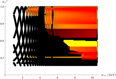
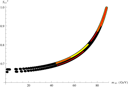
Figure 1: Constraints in the planes defined by $(m_{a^{0}_{1}},S_{13}^{2})$ (left-hand side) and $(m_{h_{1}^{0}},S_{13}^{2})$ (right-hand side) for $\mu_{\mbox{\tiny eff}}=300$ GeV. Black dots correspond to the points on which we perform the scan (without collider constraints); yellow dots are allowed by NMSSMTools_3.2.0 while red dots signal points allowed with self-Higgs couplings defined as in our procedure NMSSMTools*.

Admittedly, the modification is essentially a fringe effect and one needs to go to a region of the parameter space where the Higgs self-couplings intervene very finely to discover substantial deviation between the two approaches. We thus consider a specific region in the NMSSM parameter space, characterized by a light CP-even Higgs with mass typically under $100$ GeV, sizeable singlet-doublet mixing $S_{13}^{2}\sim 0-100\%$ and a light CP-odd Higgs with mass $<10.5$ GeV, allowing for $h^{0}_{1}\to 2a^{0}_{1}$ decays. Such a scenario is possible e.g. in an approximate Peccei-Quinn limit $\frac{\kappa}{\lambda}\ll 1$, with the parameters (NMSSMTools input: refer to [31, 32]; we use the index ‘sferm’ to denote any of the sfermions): $\tan\beta=5$, $\lambda=0.5$, $\kappa=0.05$, $6M_{1}=3M_{2}=M_{3}=1.2\leavevmode\nobreak\ \mbox{TeV}=m_{\rm sferm.}=-A_{\rm sferm.}$, $\mu_{\mbox{\tiny eff}}\in[100;900]$ GeV, $|A_{\kappa}|<30$ GeV and $M_{A}\in[0;4]$ TeV. Incidentally for those points, the doublet-like state $h_{i}^{0}$ ($i=1$ or $2$, depending on the specific point) reaches a mass of $\sim 125$ GeV in the limit of singlet-doublet decoupling $S_{i3}^{2}\sim 0$. Note however that we did not specifically attempt to preserve this feature of a Higgs state at $125$ GeV (so that for significant mixing, we may have typically $m_{h_{1}^{0}}^{2}\sim 90$ GeV while $m_{h_{2}^{0}}^{2}\sim 150$ GeV): we simply mean to show that our procedure is liable to affect the output of NMSSMTools. Note finally that, for simplicity, we discard constraints from $(g-2)_{\mu}$, which may be taken care of separately, by tuning the slepton sector. All other collider constraints – from LEP, $B/\Upsilon$-physics, TeVatron or early LHC data – within NMSSMTools_3.2.0 are kept.

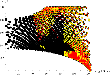
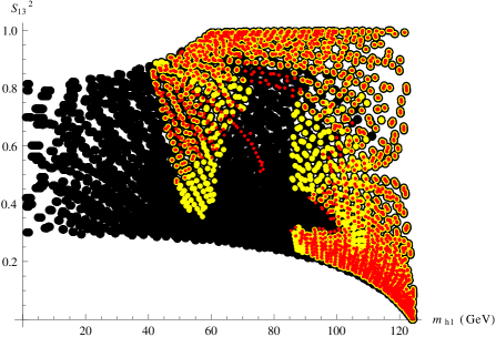
Figure 2: Constraints in the plane defined by $(m_{h_{1}^{0}},S_{13}^{2})$ for $\mu_{\mbox{\tiny eff}}\in[100;900]$ GeV. On the left-hand side, the scan with the yellow dots uses tree-level Higgs couplings, while the corresponding one on the right-end side is obtained with the couplings implemented in NMSSMTools, adding fermion corrections. The color code is otherwise similar to that of the previous figure.

We first specialize to the case $\mu_{\mbox{\tiny eff}}=300$ GeV: the lightest CP-even Higgs is then dominantly singlet ($S_{13}^{2}\sim 70-100\%$). We display our results for this scenario in Fig.1. The black dots represent points on which we scanned (with no collider constraints applied; note that their distribution is an artifact of the scan and should not be paid particular attention), the yellow dots, the output of NMSSMTools with the original Higgs couplings. Our results (NMSSMTools*), with corrected Higgs couplings, are depicted by the red dots. Since we scan over two variables, the output is two-dimensional in the $(m_{a^{0}_{1}},S_{13}^{2})$-plane. In the plane $(m_{h_{1}^{0}},S_{13}^{2})$, the constraint $m_{a^{0}_{1}}<10.5\leavevmode\nobreak\ \mbox{GeV}\ll m_{h_{1}^{0}}$ reduces the apparent dimensionality to $1$. To investigate the whole $(m_{h_{1}^{0}},S_{13}^{2})$-plane, one may additionally scan on the parameter $\mu_{\mbox{\tiny eff}}$, which we show on Fig.2. There, however, the plot on the left-hand side corresponds to the case of purely tree-level couplings (for the yellow dots), which we obtained by removing the fermion-corrections from the original couplings implemented in NMSSMTools. The obvious conclusion is that, although partially compatible, the yellow and red dots do not exactly coincide, so that the details of the constraints are affected by our procedure. Note that both points admitted by NMSSMTools while excluded by NMSSMTools* and points admitted by NMSSMTools* while excluded by NMSSMTools are to be found.

We insist however on the fact that such displacement effects in the acceptable points of the parameter space are noticeable only because we considered a region where phenomenological constraints on the Higgs spectrum and decays are particularly severe, due to the presence of very light Higgs-states which need to be sufficiently ‘invisible’ to escape experimental limits. A slight perturbation of the $\lambda_{i}$’s is then liable to result into insufficient $h_{i}^{0}\to 2a_{1}^{0}$ (‘invisible’) branching ratio, excessive decays into e.g. SM-fermions and/or excessive $a_{1}^{0}$-signals in $B$-physics: in such cases, an increased ‘invisibility’ of the light Higgs states, that is increased singlet components, is required. If, on the contrary, the perturbation of the $\lambda_{i}$’s stabilizes the invisibility of the light Higgs states, additional parameter space becomes available.Given the sensitivity of such regions to perturbations and the complex interplay of constraints at stake there, it is very difficult to predict to which extent the allowed parameter space would be shifted or not. In any case, a detailed new analysis on the NMSSM parameter space is beyond the scope of this work. Our procedure simply ensures the consistency of the calculation at leading-log order, the couplings being adequately related to the spectrum.

3.2 Implementation in SloopS

In SloopS, the complete spectrum and set of vertices are generated at tree-level from the NMSSM – SUSY and soft – parameters through the LanHEP package[49]. There, $g$, $g^{\prime}$, $v_{u}$, $v_{d}$ are determined by the physical input $M_{Z}$, $M_{W}$, $v$ and $\tan\beta$. Then the radiative part of the Higgs potential needs to be implemented: the tree-level Higgs parameters $\lambda_{i}^{0}$, given in Eq.(1.5), are thus shifted as $\lambda_{i}=\lambda_{i}^{0}+\Delta\lambda_{i}$, $\Delta\lambda_{i}$ defining the radiative corrections to the parameters $\lambda_{i}$ of Eq.(1.4). Yet, the corrected Higgs masses are not computed within SloopS, but imported from NMSSMTools through the SLHA interface. Applying the inversion procedure (Eqs.(A.1.A.2)), we obtain the $\mathbb{Z}_{3}$-invariant $\Delta\lambda_{i}$’s from the inputed masses, diagonalizing angles and tree level $\lambda_{i}^{0}$’s. From now on we will call this procedure the ‘effective physical potential approach’ and refer to it through the acronym ‘PhA’. The complete set of Feynman rules is then derived automatically in the FormCalc[50] conventions, the latter performing the calculation of the decay width.

A powerful feature of SloopS is the ability to check gauge invariance of results through a generalized non-linear gauge fixing, which was adapted to the NMSSM [37]. The gauge-fixing Lagrangian can be written in a general form

$${\mathcal{L}}_{GF}=-\frac{1}{\xi_{W}}F^{+}F^{-}-\frac{1}{2{{\xi_{Z}}}}|F^{Z}|^{2}-\frac{1}{2{{\xi_{A}}}}|F^{A}|^{2}$$ (3.1)

where the non-linear functions of the fields $F$ are given by

$$F^{+} = \bigg{(}\partial_{\mu}-ie{\tilde{\alpha}}A_{\mu}-igc_{W}{\tilde{\beta}}Z_{\mu}\bigg{)}W^{\mu\,+}$$

$$+i{{\xi_{W}}}\frac{g}{2}\bigg{(}v+{\tilde{\delta}}_{1}H_{1}+{\tilde{\delta}_{2}}H_{2}+{\tilde{\delta}_{3}}H_{3}+i({\tilde{\kappa}}G^{0}+{\tilde{\rho}}_{1}A_{1}+{\tilde{\rho}}_{2}A_{2})\bigg{)}G^{+}$$

$$F^{Z} = \partial_{\mu}Z^{\mu}+{{\xi_{Z}}}\frac{g}{2c_{W}}\bigg{(}v+{\tilde{\epsilon}}_{1}H_{1}+{\tilde{\epsilon}}_{2}H_{2}+{\tilde{\epsilon}}_{3}H_{3}\bigg{)}G^{0}$$ (3.2)

$$F^{A} = \partial_{\mu}A^{\mu}$$

The parameters $\tilde{\alpha},\tilde{\beta},\cdots,\tilde{\epsilon}_{3}$ are generalized gauge-fixing parameters. We also set $\xi_{A,Z,W}=1$ to keep a simple form for the gauge boson propagators.

The ghost Lagrangian $\mathcal{L}_{Gh}$ is established by requiring that the full effective Lagrangian is invariant under BRST transformations. This implies that the full quantum Lagrangian, with $\mathcal{L}_{C}$ the classical Lagrangian,

$$\mathcal{L}_{Q}=\mathcal{L}_{C}+\mathcal{L}_{GF}+\mathcal{L}_{Gh}$$ (3.3)

be such that $\delta_{\mbox{\tiny BRS}}\mathcal{L}_{Q}=0$ and hence $\delta_{\mbox{\tiny BRS}}\mathcal{L}_{GF}=-\delta_{\mbox{\tiny BRS}}\mathcal{L}_{Gh}$ [51]. The BRST transformation for the gauge fields can be found for example in [51]. The NMSSM specific transformations for the scalar fields can be found in [37]. For the decay $h_{i}^{0}\rightarrow\gamma\gamma$ not all the parameters are relevant: only $\tilde{\alpha}$ and $\tilde{\delta}_{i}$ are.

3.3 The decay $H\rightarrow\gamma\gamma$

The diphoton decay is an interesting process to investigate due to the relevance of this channel in the recent discovery at LHC and because the gauge invariance is fully at play there. Indeed, in the SM, the W-boson loop, together with the top-quark one (the latter being of course gauge invariant, as the remaining contributions), dominate the decay. The calculation of the diphoton rate in the non-linear gauge was originally performed in [52] in order to simplify the calculation of the Higgs decay into two photons in the SM. In short details, with the specific choice $\tilde{\alpha}=-1$, the $W^{\pm}G^{\mp}\gamma$ coupling vanishes and the gauge-boson loop calculation is made easier. In our calculation we will refrain from adopting this choice in order to preserve the ability of checking the cancellation of the unphysical gauge-dependent part in the gauge loops. We will discuss this effect only at one-loop order, meaning that we consider only the LO decay width: this will be sufficient for our purposes since we do not aim at a more precise evaluation. Nevertheless it is worth reminding that the full two-loop EW+QCD corrections for the SM-like Higgs decay into $\gamma\gamma$ are known and under 2% [53] below the WW threshold. The full two-loop SUSY corrections are as yet unknown and anyway, our procedure would not be suited for such a calculation as the renormalization of the tree level Higgs potential would be mandatory whereas our renormalization is effective and explicitly breaks SUSY. We only aim at showing how one may consistently use the radiatively corrected Higgs masses for an improved LO calculation of this decay.

Once we trade the “$\lambda_{i}$” parameters for the masses, using Eqs.(A.1,A.2), we can re-express the Higgs self-couplings, obtained from the restricted $\mathbb{Z}_{3}$-invariant potential, in terms of them. From now we will call “$\lambda$-representation” of the trilinear Higgs couplings their expression in terms of the $\lambda_{i}$’s. Moreover, when the $\lambda_{i}$’s are explicitly replaced by Higgs masses, v.e.v’s and mixing angles, we will speak of “mass-representation”. As far as the diphoton signal is concerned, the relevant couplings are those connecting the CP-even Higgs with the charged ones but also with the charged Goldstones. In the mass representation they are given by

$$g_{h_{i}^{0}H^{+}H^{-}} = \frac{1}{v\sqrt{2}}\left\{m^{2}_{h^{0}_{i}}\left(\frac{\sin\!\beta^{2}}{\cos\!\beta}S_{i1}+\frac{\cos\!\beta^{2}}{\sin\!\beta}S_{i2}\right)+2m_{H^{\pm}}^{2}(\cos\!\beta S_{i1}+\sin\!\beta S_{i2})\right.$$ (3.4)

$$\left.-\frac{2m_{a^{0}_{j}}^{2}P^{\prime}_{j1}P^{\prime}_{j2}S_{i3}}{3\sin 2\beta}-m_{a^{0}_{j}}^{2}P^{{}^{\prime}\,2}_{j1}\left(\frac{S_{i1}}{\cos\!\beta}+\frac{S_{i2}}{\sin\!\beta}-\frac{4}{3}\frac{v}{s}S_{i3}\right)\right\}$$

$$g_{h_{i}^{0}G^{+}G^{-}} = \frac{1}{v\sqrt{2}}\left\{m^{2}_{h^{0}_{i}}(\cos\!\beta S_{i1}+\sin\!\beta S_{i2})+2M_{W}^{2}{\tilde{\delta}_{i}}\right\}$$

where $m^{2}_{h^{0}_{i}}$, $m^{2}_{a^{0}_{i}}$ and $m^{2}_{H^{\pm}}$ are the physical masses and the mixing elements $S_{ij},P^{{}^{\prime}}_{ij}$ form the matrices diagonalizing the effective mass matrices Eqs.(1.20,1.22). Note also that in the non-linear gauge the $h_{i}^{0}G^{+}G^{-}$ couplings depend explicitly on the gauge through the parameters $\tilde{\delta}_{i}$. These parameters also appear within the ghost sector in the couplings $h_{i}^{0}\bar{c}^{\pm}c^{\pm}$, where $\bar{c}^{\pm},c^{\pm}$ are the charged ghost fields. The non-linear gauge parameter $\tilde{\alpha}$ also appears in the course of the calculation. It originates from couplings with physical fields like $W^{\pm}W^{\mp}\gamma$, $W^{\pm}W^{\mp}\gamma\gamma$ and unphysical ones: $G^{\pm}W^{\mp}\gamma$, $\bar{c}^{\pm}c^{\mp}\gamma$, $\bar{c}^{\pm}c^{\mp}\gamma\gamma$ (see for example [51]). The latter quartic coupling emerges from the non-linear gauge condition only. All these couplings arise purely from the ghost and Goldstone part of the gauge sector and are not modified by the effective potential of the Higgs sector.

For the numerical evaluation, as explained before, we obtain the Higgs masses and the mixing elements from NMSSMTools and the values are fed into SloopS through the SLHA interface. Here we use the second possibility offered by NMSSMTools, to compute the Higgs masses following[48]. There pole-mass corrections can be taken into account or not. In both cases the mixing matrices are computed in the effective potential approximation (i.e at $p^{2}=0$ where $p$ is the external momentum entering the Higgs self-energies).

As an illustration of the gauge invariance of the parameter reconstruction (Eqs.(A.1,A.2)), we considered two benchmark points from [54], named NMP2 and NMP5 after the conventions in [54]. Their respective Higgs sector parameters are recalled in Table 1, together with the soft SUSY breaking masses of the stop sector $M_{\tilde{Q}_{L}^{3}}$, $M_{\tilde{t}_{R}}$ and of the gluino sector $M_{3}$. All remaining soft masses and trilinear parameters that are not given in Table 1 are set at 1 TeV.

Parameter	NMP2	NMP5
$\tan\beta$	2	3
$\lambda$	0.6	0.66
$\kappa$	0.18	0.12
$\mu_{\rm eff.}$ [GeV]	200	200
$A_{\lambda}$ [GeV]	405	650
$A_{\kappa}$ [GeV]	-10	-10
$M_{\tilde{Q}^{3}_{L}}$ [GeV]	700	600
$M_{\tilde{t}_{R}}$ [GeV]	700	600
$M_{3}$ [GeV]	600	600

Table 1: Benchmark points taken from [54] for the diphoton decay width.

The resulting Higgs spectrum is summarized in Table 2 and computed within NMSSMTools according to the procedure [48] with and without the pole-mass corrections.

Mass	NMP2		NMP5
$\rm[GeV]$	no pole	pole	no pole	pole
$m_{h_{1}^{0}}$	129.4	126.5	96.1	95.6
$m_{h_{2}^{0}}$	133.1	132.4	128.9	126.5
$m_{h_{3}^{0}}$	470.8	464.5	659.9	655.8
$m_{a_{1}^{0}}$	116.4	115.7	93.9	93.2
$m_{a_{2}^{0}}$	468.7	462.8	660.1	656.5
$m_{H^{\pm}}$	454.4	454.5	644.8	644.9

Table 2: Higgs spectrum of the benchmark points considered. For the NMP2 point the lightest CP-even Higgs is SM-like and for NMP5 it is the second-to-lightest one.

In addition to the masses given in the SLHA output we also need the mixing elements $S_{ij}$ and $P^{\prime}_{ij}$ to obtain the couplings entering the diphoton decay width. In the effective potential approach used in [48], that we henceforth denote as EPA, they are obtained by diagonalizing the radiatively corrected Higgs mass matrices in the $\overline{\rm DR}$-scheme anew. However the definition of the diagonalizing matrices is ambiguous since the self energies entering the radiatively corrected mass matrices depend on the external momentum. In [48] the rotations matrices are defined as those that diagonalize the mass matrices at $p^{2}=0$. Then, whether pole-mass corrections are taken into account or not leads to the same diagonalization matrices $S$ and $P^{\prime}$: This can be seen formally as a missing higher-order correction, but, in this fashion, the physical Higgs mass matrix would not correspond to the $\overline{\rm DR}$ one in the EPA. This inconvenience is circumvented in the physical effective approach (PhA) as we force the radiatively corrected mass matrices to be the physical ones by imposing Eqs.(A.1,A.2).

To reproduce the EPA method using pole-masses within SloopS, we take the $\overline{\rm DR}$-masses for the reconstruction of the potential of Eq.(1.4) but the pole masses for the kinematics of the process. Therefore the Higgs mass appearing in the coupling of Eq.(3.4) is the $\overline{\rm DR}$-mass, which differs from the energy at which the decay is evaluated. This mismatch in the EPA with pole-masses will lead to a violation of gauge invariance within our generalized non-linear gauge, as we will show numerically. On the other hand, in the PhA, we reconstruct the potential of Eq.(1.4) (and consequently the Higgs mass matrices as well) directly from the pole-masses, which are also still used in the kinematics. This procedure will guarantee that gauge invariance is maintained because Eqs.(A.1,A.2) are fulfilled. At the numerical level we will vary the parameters $\tilde{\alpha},\tilde{\delta}_{i}$ within SloopS to exemplify the gauge-invariance of the calculation in the PhA method. The results are presented in Table 3. They were cross-checked with the standard NMSSMTools version and with NMSSMTools*. The corresponding output of NMSSMTools, whether in the standard or modified version, does not check internally any consistency requirement, such as gauge-invariance, and simply uses an analytic, pre-computed expression for the effective $h_{i}^{0}\gamma\gamma$ couplings.

NMP2
$\Gamma(h_{1}^{0}\rightarrow\gamma\gamma)$	$\tilde{\alpha}=\tilde{\delta}_{1}=0$	$\tilde{\alpha}=\tilde{\delta}_{1}=10$
SloopS (EPA)	1.138108952362$.\,10^{-5}$	4.490893854783$.\,10^{-5}$
SloopS (PhA)	1.125710969262$.\,10^{-5}$	1.125710969261$.\,10^{-5}$
NMSSMTools_3.2.0	1.12699441$.\,10^{-5}$
NMSSMTools*	1.12737737$.\,10^{-5}$
NMP5
$\Gamma(h_{2}^{0}\rightarrow\gamma\gamma)$	$\tilde{\alpha}=\tilde{\delta}_{2}=0$	$\tilde{\alpha}=\tilde{\delta}_{2}=10$
SloopS (EPA)	1.053756232511$.\,10^{-5}$	3.628709516521$.\,10^{-5}$
SloopS(PhA)	1.044860481657$.\,10^{-5}$	1.044860481613$.\,10^{-5}$
NMSSMTools_3.2.0	1.04342526$.\,10^{-5}$
NMSSMTools*	1.04361857$.\,10^{-5}$

Table 3: Gauge invariance test for the computation of $\Gamma(h_{1,2}^{0}\rightarrow\gamma\gamma)$ (in GeV) in the EPA and PhA procedures. Only the PhA approach passes the gauge invariance test within SloopS. There is no such test available with NMSSMTools, whether it is the modified version or not.

The excellent agreement among the results of NMSSMTools and the computation of SloopS for vanishing non-linear gauge parameters (i.e. in a linear gauge) is therefore a welcomed feature. The sources for possible discrepancies between SloopS and NMSSMTools lie in the treatment of the sfermion sector: in SloopS it is treated purely at tree-level whereas NMSSMTools includes several corrections to the spectrum and couplings[32]. For the two benchmark points investigated this difference is almost invisible because the sfermion sector is essentially decoupled.

These illustrative examples show however evidently that the EPA calculation is not gauge-invariant. The origin of this breakdown can be traced back to the observation that Eqs.(A.1,A.2) are not satisfied. In more restricted gauges the gauge dependence would be seen at higher orders only. As stated above, setting $\tilde{\alpha}=-1$ removes the $G^{\pm}W^{\mp}\gamma$ coupling and varying $\tilde{\delta}_{1,2}$ then gives gauge-invariant results in both procedures: they differ only by a finite and gauge-independent piece. This is due to the fact that the $\tilde{\delta}_{1,2}$ gauge-dependent parts only appear proportionally to $M_{W}^{2}/v\sqrt{2}$. On the contrary, in the general case, $\tilde{\alpha}$-dependent parts are proportional to the Higgs mass $m_{h_{i}^{0}}$, originating from the kinematics (i.e. the center of mass energy $\sqrt{s}$), and the $g_{h_{i}^{0}G^{+}G^{-}}$ coupling, see Eq.(3.4). Recall that in the EPA the mass appearing in the coupling $g_{h_{i}^{0}G^{+}G^{-}}$ is not equal to the pole-mass, which is used for the on-shell decay. The gauge-dependence of the EPA is precisely caused by this mismatch between the “kinematical” mass and the mass appearing in the coupling of Eq.(3.4) if pole-mass corrections are applied. In the opposite case, that of the PhA, the “kinematical” mass and the one appearing in the coupling are the same and the gauge dependent part $\propto\tilde{\alpha}$ vanishes. We can render the EPA approach gauge-invariant if no pole-mass corrections are applied (this would then be a ‘PhA with $\overline{DR}$-masses’). However, in this last case some precision is lost since, looking back to Table 2, there is a 2-3 GeV mass difference between pole and running masses. Within our reconstruction, the charged Higgs contribution is modified through the $g_{h_{i}^{0}H^{+}H^{-}}$ coupling: we do not expect significant modifications with respect to previous calculations, in the MSSM-limit of the NMSSM, since it is known that the charged Higgs contribution to the diphoton decay width in the MSSM remains small (see for example [12]). In the NMSSM with large $\lambda$ (a form of the so-called ‘$\lambda$-SUSY’ models [16], which typically leads to a Landau pole below the GUT scale) and a relatively light charged Higgs mass, one could modify significantly $g_{h_{i}^{0},H^{+}H^{-}}$, without requiring large doublet-singlet mixing. This was explicitly shown in [55].

Note however that a serious issue would arise with the gauge-dependent calculation of $h_{i}^{0}\rightarrow\gamma\gamma$ if one would choose to use it in order to derive some fundamental parameters at the Lagrangian level, which should preferably be determined from gauge-independent observables. As a final remark concerning this section, beyond maintaining gauge invariance, the PhA is clearly advantageous as it enables us to use the pole-masses easily in the calculation of the decay width, in a consistent way, without resorting to the technical task of computing the “pole-corrected” mixing elements $S_{ij},P^{\prime}_{ij}$.

3.4 Comparison with micrOMEGAs

A comparable approach, based on an effective potential approach, had been carried out in micrOMEGAs [33, 34], a code computing the DM relic density $\Omega_{\chi}h^{2}$ in (e.g.) the NMSSM. Since light Higgs states can be present, annihilation channels into $h_{1}^{0}h_{1}^{0}$, $h_{1}^{0}a_{1}^{0}$, $a_{1}^{0}a_{1}^{0}$ can contribute significantly to $\Omega_{\chi}h^{2}$ and such channels are affected by radiative corrections in the Higgs sector. The effective scalar potential was implemented in this code as (see [34], where a slightly different version was proposed),

$${\cal V}_{\rm rad} = \lambda_{1}^{M}|H_{u}|^{2}+\lambda_{2}^{M}|H_{d}|^{2}+\lambda_{3}^{M}|H_{u}|^{2}|H_{d}|^{2}+\lambda_{4}^{M}|H_{u}\cdot H_{d}|^{2}+\frac{\lambda_{5}^{M}}{2}\left[(H_{u}\cdot H_{d})^{2}+h.c\right]$$ (3.5)

$$+ \lambda_{1}^{s}|S|^{2}|H_{u}|^{2}+\lambda_{2}^{s}|S|^{2}|H_{d}|^{2}+\left[\frac{\lambda_{5}^{s}}{2}S^{2}(H_{u}\cdot H_{d})+\lambda^{s}_{p}S^{4}+h.c\right]+\frac{\lambda^{s}_{s}}{2}|S|^{4}$$

This potential is to be understood as a radiative potential, which means that all the parameters are loop-induced. To make a connection with our conventions we have

$$\Delta\lambda_{1}=\lambda_{2}^{M}\,,\Delta\lambda_{2}=\lambda_{1}^{M}\,,\Delta\lambda_{3}=\lambda_{3}^{M}\,,\Delta\lambda_{4}=\lambda_{4}^{M}\,,\Delta\lambda_{P}^{u}=\lambda_{1}^{s}\,,\Delta\lambda_{P}^{d}=\lambda_{2}^{s}\,,\Delta\kappa^{2}=\lambda_{s}^{s}$$ (3.6)

where the $\Delta\lambda_{i}$ are the loop-induced part of the $\lambda_{i}$ parameters appearing in Eq.(1.4) when we split them as $\lambda_{i}=\lambda_{i}^{0}+\Delta\lambda_{i}$. The remaining parameters $\lambda^{s}_{p}$, $\lambda_{5}^{M}$, and $\lambda_{5}^{s}$ have no equivalent in our restricted potential of Eq.(1.4), but correspond, in our conventions for the general potential (Eq.1.2), to

$$\lambda_{5}^{M}=\lambda_{5},\,\lambda^{s}_{p}={\tilde{\kappa}}^{2}_{S}/4\,,\tilde{\lambda}^{M}_{P}=\lambda_{5}^{s}/2$$ (3.7)

Conversely, our parameters $A_{ud}$, $A_{S}$ and $\lambda_{P}^{M}$ receive no correction in the micrOMEGAs approach, which, obviously, does not rely on the $\mathbb{Z}_{3}$ symmetry. As a consequence, while an inversion procedure is also possible with the potential of Eq.(3.5), the radiative corrections to the masses will be distributed in a different way among the $\lambda_{i}$’s, leading to differences at the level of the Higgs self-couplings.

We remind here, that if one aims at improving on the tree-level couplings, as is obviously the purpose of a radiative potential, i.e. of Eq.(3.5), it becomes crucial to identify the $\lambda_{i}$’s that are subject to large quantum corrections: that was our discussion in subsection 2.3. An arbitrary truncation of the potential, albeit allowing for an inversion in terms of the Higgs masses provided it is sufficiently simple, is not a receivable option because the accuracy contained within the couplings brings no improvement with respect to the tree-level evaluation. Our study of the large logarithms within the Coleman-Weinberg approach tends to convince us that our choice of a $\mathbb{Z}_{3}$-invariant potential should be preferred, while the choice in Eq.(3.5) seems arbitrary. Possible reasons for this choice within micrOMEGAs could lie on the facts that the loop-corrections to $\lambda_{5}$ are sizeable in the MSSM, and one could have expected the same behavior in the NMSSM, while the parameters $\lambda^{s}_{p}$ and $\lambda_{5}^{s}$ (or rather $\tilde{\kappa}_{S}^{2}$ and $\tilde{\lambda}_{P}^{M}$ in our conventions) appear in the trilinear couplings $h_{i}^{0}h_{j}^{0}h_{k}^{0}$ and $h_{i}^{0}a_{j}^{0}a_{k}^{0}$ with a factor $s$ (questionably an enhancement factor in the MSSM limit): see Eqs.(B.1,B.1). However other parameters in the general potential of Eq.(1.2) share this latter property and are still arbitrarily absent. We will see in a numerical example that ensuing deviations between our implementation and that in micrOMEGAs could be significant.

We considered a point in the NMSSM parameter space where the DM relic density $\Omega_{\chi}h^{2}$ is in the correct experimental range (at the $2\sigma$ level: $0.1\lesssim\Omega_{\chi}h^{2}\lesssim 0.124$ [56]), when computed with micrOMEGAs_2.4.1 and the Higgs radiative potential of Eq.(3.5). This specific point passes warnings from NMSSMTools_3.2.0 as well, and features a SM-like CP-even Higgs mass around 125 GeV. The NMSSMTools input for this point is given in Table 4.

Parameter	Value	Parameter	Value
$M_{1}$ [GeV]	84.49	$t_{\beta}$	2
$M_{2}$ [GeV]	359	$\lambda$	0.63
$M_{3}$ [GeV]	1200	$\kappa$	0.05
$A_{f}$ [GeV]	-1500	$A_{\lambda}$ [GeV]	694
$M_{\tilde{l}}$ [GeV]	200	$A_{\kappa}$ [GeV]	0
$M_{\tilde{q}}$ [GeV]	600	$\mu_{\rm eff.}$ [GeV]	300

Table 4: SUSY point for the comparison between micrOMEGAs, SloopS and NMSSMTools. $M_{\tilde{l}}$ and $M_{\tilde{q}}$ are common sleptons and squarks soft masses.

The main channel contributing to $\Omega_{\chi}h^{2}$ is ${\tilde{\chi}}_{1}^{0}{\tilde{\chi}}_{1}^{0}\rightarrow a_{1}^{0}a_{1}^{0}$ (at 72%) and the rest of the contributions involve fermions in the final state, dominated by the $b\bar{b}$ final state. The process ${\tilde{\chi}}_{1}^{0}{\tilde{\chi}}_{1}^{0}\rightarrow a_{1}^{0}a_{1}^{0}$ is dominated by the s-channel exchange of the SM-like Higgs $h_{2}^{0}$ close to its mass shell, as can be seen on Table 5, where the Higgs spectrum, the lightest neutralino mass $m_{{\tilde{\chi}}_{1}^{0}}$ and the resulting relic density are provided.

Spectrum
$m_{{\tilde{\chi}}_{1}^{0}}$ [GeV]	63.2
$m_{h_{1}^{0}}$ [GeV]	110.9
$m_{h_{2}^{0}}$ [GeV]	126.4
$m_{h_{3}^{0}}$ [GeV]	727.8
$m_{a_{1}^{0}}$ [GeV]	59.7
$m_{a_{2}^{0}}$ [GeV]	732.4
$m_{H^{\pm}}$ [GeV]	721.7
Relic density
$\Omega_{\chi}h^{2}$	0.103

Table 5: Resulting spectrum and $\Omega_{\chi}h^{2}$ from the data point presented in Table 4.

The decay modes $h_{2,3}^{0}\rightarrow 2a_{1}^{0}$ are kinematically open. Let us compare these decay widths within the three codes: SloopS, with our effective implementation (Eq.(A.1,A.2)), micrOMEGAs using the radiative potential in Eq.(3.5) and NMSSMTools_3.2.0, where only the leading logarithms in top/bottom corrections are taken into account. The output of NMSSMTools* is also considered. The results are displayed in Table 6.

Decay [GeV]	$\Gamma(h_{2}^{0}\rightarrow a_{1}^{0}a_{1}^{0})$	$\Gamma(h_{3}^{0}\rightarrow a_{1}^{0}a_{1}^{0})$
SloopS	$3.566\,10^{-2}$	$1.900\,10^{-4}$
micrOMEGAs_2.4.1	$2.960\,10^{-2}$	$4.665\,10^{-5}$
NMSSMTools_3.2.0	$2.730\,10^{-2}$	$1.233\,10^{-4}$
NMSSMTools*_3.2.0	$3.566\,10^{-2}$	$1.900\,10^{-4}$

Table 6: Comparison of the decay widths $h_{2,3}^{0}\rightarrow 2a_{1}^{0}$.

We observe significant discrepancies between SloopS/NMSSMTools*_3.2.0 (which are in remarkable agreement), on one side, micrOMEGAS_2.4.1/NMSSMTools_3.2.0 (which also show some disagreement between them), on the other. Our calculation for the main channel $h_{2}^{0}\rightarrow 2a_{1}^{0}$ (that we denote henceforth as $\Gamma^{S}(h_{2}^{0}\rightarrow a_{1}^{0}a_{1}^{0})$) is about a factor 1.2 larger than the micrOMEGAs result (labeled as $\Gamma^{M}(h_{2}^{0}\rightarrow a_{1}^{0}a_{1}^{0})$).

Giving the modified prediction of $\Omega_{\chi}h^{2}$ within our procedure is beyond the scope of this work, but we can nevertheless make a rough estimation of this quantity. As the process ${\tilde{\chi}}_{1}^{0}{\tilde{\chi}}_{1}^{0}\rightarrow a_{1}^{0}a_{1}^{0}$ is dominated by the $h_{2}^{0}$ resonance, and only the $h_{2}^{0}a_{1}^{0}a_{1}^{0}$ coupling is modified, we can reasonably approximate,

$$\frac{\sigma^{S}({\tilde{\chi}}_{1}^{0}{\tilde{\chi}}_{1}^{0}\rightarrow a_{1}^{0}a_{1}^{0})}{\sigma^{M}({\tilde{\chi}}_{1}^{0}{\tilde{\chi}}_{1}^{0}\rightarrow a_{1}^{0}a_{1}^{0})}\sim\frac{\Gamma^{S}(h_{2}^{0}\rightarrow a_{1}^{0}a_{1}^{0})}{\Gamma^{M}(h_{2}^{0}\rightarrow a_{1}^{0}a_{1}^{0})}\sim 1.2$$ (3.8)

Denoting $\sigma^{M}_{r}$ as the contribution of the rest of the processes to the cross-sections involved in $\Omega_{\chi}^{M}h^{2}$, the relic density computed within micrOMEGAs, we can write the sum of all contributions $\sigma_{\rm tot}^{M}({\tilde{\chi}}_{1}^{0}{\tilde{\chi}}_{1}^{0}\rightarrow X)$ as, $X$ standing for any relevant final state,

$$\sigma_{\rm tot}^{M}({\tilde{\chi}}_{1}^{0}{\tilde{\chi}}_{1}^{0}\rightarrow X)=\sum_{X}\sigma^{M}({\tilde{\chi}}_{1}^{0}{\tilde{\chi}}_{1}^{0}\rightarrow X)=\sigma^{M}({\tilde{\chi}}_{1}^{0}{\tilde{\chi}}_{1}^{0}\rightarrow a_{1}^{0}a_{1}^{0})+\sigma^{M}_{r}$$ (3.9)

The micrOMEGAs calculation gives $\sigma^{M}({\tilde{\chi}}_{1}^{0}{\tilde{\chi}}_{1}^{0}\rightarrow a_{1}^{0}a_{1}^{0})/\sigma^{M}_{\rm tot}({\tilde{\chi}}_{1}^{0}{\tilde{\chi}}_{1}^{0}\rightarrow X)=72\%$, as we already mentioned, and the ratio of relic densities in both approaches is approximately determined by $\Omega_{\chi}^{M}h^{2}/\Omega_{\chi}^{S}h^{2}\simeq\sigma^{S}_{\rm tot}/\sigma^{M}_{\rm tot}$, with $\Omega_{\chi}^{S}h^{2}$ the relic abundance in our calculation, and where

$$\sigma^{S}_{\rm tot}=\sigma^{S}({\tilde{\chi}}_{1}^{0}{\tilde{\chi}}_{1}^{0}\rightarrow a_{1}^{0}a_{1}^{0})+\sigma^{S}_{r}$$ (3.10)

Moreover we have $\sigma^{S}_{r}=\sigma^{M}_{r}$, since the remaining relevant contributions are annihilations into light fermions and hence unaffected by corrections in the Higgs sector. Thus we obtain the following estimate,

$$\Omega^{S}_{\chi}h^{2}\simeq 0.090$$ (3.11)

A reduction of the relic density with respect to the micrOMEGAs calculation was to be anticipated since in our computation the annihilation into light pseudoscalars is enhanced, thus depleting the abundance of relic neutralinos more efficiently. In turn, and contrarily to the prediction of micrOMEGAs, this point would actually lie outside the cosmologically interesting region if one relies on our estimate. Of course the derived value of $\Omega_{\chi}h^{2}$ also depends crucially on the precision of the evaluation of $m_{h_{2}^{0}}$ (and $m_{{\tilde{\chi}}_{1}^{0}}$) since the annihilation ${\tilde{\chi}}_{1}^{0}{\tilde{\chi}}_{1}^{0}\rightarrow a_{1}^{0}a_{1}^{0}$ occurs at the $h_{2}^{0}$ resonance. These considerations are of particular significance when one considers that the PLANCK satellite[57] should improve the experimental determination of cosmological parameters[58] soon. For a discussion concerning the accuracies required from colliders to match the precision of the relic density measurement, see for example [59].

Conclusions

This study of the Higgs potential with two Higgs doublets and one gauge singlet has put forward several points of interests that we would like to summarize briefly here.

The most general effective renormalizable Lagrangian of the $2$-doublet$+1$-singlet setup, contains $28$ (plus one superfluous) parameters, far beyond the $11$ ones of the 2HDM, even after complex phases have been discarded. Therefore, if future experimental measurements should point towards such a rich Higgs sector, a full reconstruction of its potential through experimental data in the Higgs sector could succeed only after an exhaustive measurement of the Higgs self-couplings, beyond that of the masses and mixing angles: if the purpose for such a reconstruction is sound from the point of view of model identification and precision tests, it is also probably condemned to a very long delay, as far as the experimental phase is concerned. This situation is eventually that of most models, albeit constrained, once considered at the radiative level, for symmetries are spontaneously broken by the Higgs v.e.v.’s and loop corrections end up contributing to all possible terms in the potential. We emphasize, however, that a precise determination, in a general parametrical form, of the potential at future (linear) colliders, shall help discriminate among such models and constrain their parameters: in turn, the predictions of specific models for the parameters of the Higgs potential should be known at the radiative level so as to allow for comparison/precision tests.

Requirements for additional symmetries, beyond the EW-invariance, or matching conditions originating from more-elaborate models may constrain the effective potential at the classical order. Provided its form is simple enough, an identification at leading order of the parameters of the underlying model is achievable from the Higgs spectrum solely. Then, assuming the remaining sectors of the model are sufficiently documented as well, a full determination of the effective potential within the more-fundamental model is essentially a matter of perturbative calculation. We lent particular attention to the $\mathbb{Z}_{3}$-invariant and PQ-conserving potentials, which could both be embedded within a SUSY extension of the SM, respectively, the NMSSM or the UMSSM, the PQ’-conserving potential (R-symmetric limit of the NMSSM) or the potential driven by an underlying nMSSM. A reconstruction of the classical parameters was explicitly carried out, at leading order, for those models.

Further achievements seemed within reach in models ensuring a residual symmetry at the EW scale. Our test-model here was the NMSSM, and the study of the large logarithms within the Coleman-Weinberg approach confirmed that the leading-logarithmic effects would not spoil the $\mathbb{Z}_{3}$-symmetry, extending the validity of our parameter reconstruction in terms of the Higgs spectrum to this order. By contrast, in the nMSSM, where no residual symmetry is present at low-energy, logarithms do not observe the classical form, spoiling a reconstruction beyond LO.

We finally considered a few phenomenological consequences of this parameter reconstruction at the leading-logarithmic order in the NMSSM. We based our discussion on the Higgs spectrum computed in the public code NMSSMTools and implemented the reconstruction both within NMSSMTools, directly, and within SloopS. The latter allowed us to visit the diphoton decay of the SM-like CP-even scalar again and clarified the conditions for a gauge-independent implementation. Comparison with the previous implementation of an effective Higgs potential within micrOMEGAs was also carried out: different choices in the radiative potential result in different Higgs-to-Higgs couplings at the order of leading logarithms, as the radiative effects encoded within the masses are distributed differently among the parameters of Eq.(1.2); while the form in Eq.(3.5) is seemingly arbitrary, our choice (Eq.(1.4)) is justified by the analysis of the logarithms appearing in the Coleman-Weinberg approach, and should thence prove a priori more reliable. As far as the phenomenology of the NMSSM is concerned, we found fine effects in collider-constraints or the calculation of the DM relic density, appearing essentially for points of the parameter space which rely heavily on Higgs-to-Higgs couplings, such as those entering the processes $h_{1}^{0}\to a_{1}^{0}a_{1}^{0}$ or ${\tilde{\chi}}_{1}^{0}{\tilde{\chi}}_{1}^{0}\to a_{1}^{0}a_{1}^{0}$, mediated by a CP-even Higgs in the s-channel.

Finally, let us mention that, although the state discovered at LHC is in a favourable mass-range for singlet-extensions of the MSSM, a long stage of experimental measurements and identifications of additional Higgs states lies ahead of us, should the $2$-doublet$+1$-singlet setup be realized at all in Nature.

Appendix A Parameter reconstruction for simple classical potentials

We provide here the results of the inversion procedure described in section 2.3 for a few classical potentials. Note that, for completeness, one should also replace the parameters within Eq.(1.3) to fully determine the potential.

$\mathbb{Z}_{3}$-invariant potential ${\cal V}^{S}_{\mathbb{Z}_{3}}$:
The quartic doublet couplings are entirely determined by the Higgs mass-matrices:

$$\begin{cases}\lambda_{1}=\frac{1}{2v^{2}}\left[\frac{m^{2}_{h_{i}^{0}}S_{i1}^{2}}{\cos^{2}\beta}-m^{2}_{a_{i}^{0}}P^{\prime 2}_{i1}\tan^{2}\beta\right]\\ \lambda_{2}=\frac{1}{2v^{2}}\left[\frac{m^{2}_{h_{i}^{0}}S_{i2}^{2}}{\sin^{2}\beta}-\frac{m^{2}_{a_{i}^{0}}P^{\prime 2}_{i1}}{\tan^{2}\beta}\right]\\ \lambda_{3}=\frac{1}{2v^{2}}\left[2m_{H^{\pm}}^{2}+\frac{2m^{2}_{h_{i}^{0}}S_{i1}S_{i2}}{\sin 2\beta}-m^{2}_{a_{i}^{0}}P^{\prime 2}_{i1}\right]\\ \lambda_{4}=\frac{1}{v^{2}}\left[m^{2}_{a_{i}^{0}}P^{\prime 2}_{i1}-m_{H^{\pm}}^{2}\right]\end{cases}$$ (A.1)

One degree of freedom remains, which can be chosen conveniently as the singlet v.e.v. $s$. One then obtains for the remaining parameters:

$$\begin{cases}A_{ud}=\frac{1}{3}\left[\frac{\sin 2\beta}{s}m^{2}_{a_{i}^{0}}P^{\prime 2}_{i1}+\frac{1}{v}m^{2}_{a_{i}^{0}}P^{\prime}_{i1}P^{\prime}_{i2}\right]\\ \lambda_{P}^{M}=\frac{1}{3s}\left[\frac{\sin 2\beta}{2s}m^{2}_{a_{i}^{0}}P^{\prime 2}_{i1}-\frac{1}{v}m^{2}_{a_{i}^{0}}P^{\prime}_{i1}P^{\prime}_{i2}\right]\\ A_{S}=\frac{1}{3s}\left[\frac{v^{2}\sin^{2}2\beta}{2s^{2}}m^{2}_{a_{i}^{0}}P^{\prime 2}_{i1}-m^{2}_{a_{i}^{0}}P^{\prime 2}_{i2}-\frac{v\sin 2\beta}{2s}m^{2}_{a_{i}^{0}}P^{\prime}_{i1}P^{\prime}_{i2}\right]\\ \kappa^{2}=\frac{1}{4s^{2}}\left[m_{h_{i}^{0}}^{2}S_{i3}^{2}+\frac{1}{3}m^{2}_{a_{i}^{0}}P^{\prime 2}_{i2}-\frac{v^{2}\sin^{2}2\beta}{3s^{2}}m^{2}_{a_{i}^{0}}P^{\prime 2}_{i1}\right]\\ \lambda_{P}^{u}=\frac{m_{h_{i}^{0}}^{2}S_{i2}S_{i3}}{2sv\sin\beta}+\frac{1}{3s\tan\beta}\left[\frac{\sin 2\beta}{s}m^{2}_{a_{i}^{0}}P^{\prime 2}_{i1}-\frac{1}{2v}m^{2}_{a_{i}^{0}}P^{\prime}_{i1}P^{\prime}_{i2}\right]\\ \lambda_{P}^{d}=\frac{m_{h_{i}^{0}}^{2}S_{i1}S_{i3}}{2sv\cos\beta}+\frac{\tan\beta}{3s}\left[\frac{\sin 2\beta}{s}m^{2}_{a_{i}^{0}}P^{\prime 2}_{i1}-\frac{1}{2v}m^{2}_{a_{i}^{0}}P^{\prime}_{i1}P^{\prime}_{i2}\right]\end{cases}$$ (A.2)

In replacement of $s$, one may use any combination of these latter equations to define a new parameter. For instance,

$$\varepsilon_{(a,b)}\equiv\frac{\lambda_{P}^{M}(a+b)}{a\lambda_{P}^{u}+b\lambda_{P}^{d}}\hskip 28.45274pt\Leftrightarrow\\ s=\frac{v\sin 2\beta\,m^{2}_{a_{i}^{0}}P^{\prime 2}_{i1}\left[1-2\varepsilon_{(a,b)}\left(\frac{a}{\tan\beta}+b\tan\beta\right)\right]}{2m^{2}_{a_{i}^{0}}P^{\prime}_{i1}P^{\prime}_{i2}\left[1-\frac{\varepsilon_{(a,b)}}{2}\left(\frac{a}{\tan\beta}+b\tan\beta\right)\right]+3\varepsilon_{(a,b)}m_{h_{i}^{0}}^{2}S_{i3}\left(a\frac{S_{i1}}{\sin\beta}+b\frac{S_{i2}}{\cos\beta}\right)}$$ (A.3)

$\varepsilon_{(a,b)}$ coincides with $\kappa/\lambda$ in the NMSSM at tree-level and may be regarded as a measurement of the breakdown of the Peccei-Quinn symmetry. Alternatively,

$$\rho_{ud}\equiv\frac{\lambda_{P}^{u}}{\lambda_{P}^{d}}-1\hskip 28.45274pt\Leftrightarrow\\ s=\frac{2v\sin 2\beta\,m_{a_{i}^{0}}^{2}P^{\prime 2}_{i1}\left[1-(1+\rho_{ud})\tan^{2}\beta\right]}{m_{a_{i}^{0}}^{2}P^{\prime}_{i1}P^{\prime}_{i2}\left[1-(1+\rho_{ud})\tan^{2}\beta\right]-3m_{h_{i}^{0}}^{2}S_{i3}\left[\frac{S_{i1}}{\cos\beta}-(1+\rho_{ud})\tan^{2}\beta\frac{S_{i2}}{\sin\beta}\right]}$$ (A.4)

$\rho_{ud}$ vanishes at tree-level in the NMSSM and may represent another possibility.

Peccei-Quinn-invariant potential ${\cal V}^{S}_{PQ}$:
The system is fully determined by the mass matrices:

$$\begin{cases}\lambda_{1}=\frac{1}{2v^{2}}\left[\frac{m^{2}_{h_{i}^{0}}S_{i1}^{2}}{\cos^{2}\beta}-m^{2}_{a_{2}^{0}}P^{\prime 2}_{21}\tan^{2}\beta\right]\\ \lambda_{2}=\frac{1}{2v^{2}}\left[\frac{m^{2}_{h_{i}^{0}}S_{i2}^{2}}{\sin^{2}\beta}-\frac{m^{2}_{a_{2}^{0}}P^{\prime 2}_{21}}{\tan^{2}\beta}\right]\\ \lambda_{3}=\frac{1}{2v^{2}}\left[2m_{H^{\pm}}^{2}+\frac{2m^{2}_{h_{i}^{0}}S_{i1}S_{i2}}{\sin 2\beta}-m^{2}_{a_{2}^{0}}P^{\prime 2}_{21}\right]\\ \lambda_{4}=\frac{1}{v^{2}}\left[m^{2}_{a_{2}^{0}}P^{\prime 2}_{21}-m_{H^{\pm}}^{2}\right]\\ A_{ud}=\frac{m^{2}_{a_{2}^{0}}P^{\prime}_{21}P^{\prime}_{22}}{v}\\ s=\frac{v}{2}\sin{2\beta}\frac{P^{\prime}_{21}}{P^{\prime}_{22}}\\ \kappa^{2}=\frac{(P^{\prime}_{22}/P^{\prime}_{21})^{2}}{v^{2}\sin^{2}2\beta}\left[m_{h_{i}^{0}}^{2}S_{i3}^{2}-m^{2}_{a_{2}^{0}}P^{\prime 2}_{22}\right]\\ \lambda_{P}^{u}=\frac{1}{2v^{2}\sin^{2}\beta}\frac{P^{\prime}_{22}}{P^{\prime}_{21}}\left[\frac{m_{h_{i}^{0}}^{2}S_{i2}S_{i3}}{\cos{\beta}}+m^{2}_{a_{2}^{0}}P^{\prime}_{21}P^{\prime}_{22}\right]\\ \lambda_{P}^{d}=\frac{1}{2v^{2}\cos^{2}\beta}\frac{P^{\prime}_{22}}{P^{\prime}_{21}}\left[\frac{m_{h_{i}^{0}}^{2}S_{i1}S_{i3}}{\sin{\beta}}+m^{2}_{a_{2}^{0}}P^{\prime}_{21}P^{\prime}_{22}\right]\end{cases}$$ (A.5)

Peccei-Quinn’-invariant potential ${\cal V}^{S}_{PQ^{\prime}}$:
The system is fully determined by the mass matrices:

$$\begin{cases}\lambda_{1}=\frac{1}{2v^{2}}\left[\frac{m^{2}_{h_{i}^{0}}S_{i1}^{2}}{\cos^{2}\beta}-m^{2}_{a_{2}^{0}}P^{\prime 2}_{21}\tan^{2}\beta\right]\\ \lambda_{2}=\frac{1}{2v^{2}}\left[\frac{m^{2}_{h_{i}^{0}}S_{i2}^{2}}{\sin^{2}\beta}-\frac{m^{2}_{a_{2}^{0}}P^{\prime 2}_{21}}{\tan^{2}\beta}\right]\\ \lambda_{3}=\frac{1}{2v^{2}}\left[2m_{H^{\pm}}^{2}+\frac{2m^{2}_{h_{i}^{0}}S_{i1}S_{i2}}{\sin 2\beta}-m^{2}_{a_{2}^{0}}P^{\prime 2}_{21}\right]\\ \lambda_{4}=\frac{1}{v^{2}}\left[m^{2}_{a_{2}^{0}}P^{\prime 2}_{21}-m_{H^{\pm}}^{2}\right]\\ \lambda_{P}^{M}=\frac{m^{2}_{a_{2}^{0}}P^{\prime 2}_{22}}{2v^{2}\sin{2\beta}}\\ s=-v\sin{2\beta}\frac{P^{\prime}_{21}}{P^{\prime}_{22}}\\ \kappa^{2}=\frac{m_{h_{i}^{0}}^{2}S_{i3}^{2}}{4v^{2}\sin^{2}2\beta}\left(\frac{P^{\prime}_{22}}{P^{\prime}_{21}}\right)^{2}\\ \lambda_{P}^{u}=\frac{1}{4v^{2}\sin^{2}\beta}\frac{P^{\prime}_{22}}{P^{\prime}_{21}}\left[m^{2}_{a_{2}^{0}}P^{\prime}_{21}P^{\prime}_{22}-\frac{m_{h_{i}^{0}}^{2}S_{i2}S_{i3}}{\cos{\beta}}\right]\\ \lambda_{P}^{d}=\frac{1}{4v^{2}\cos^{2}\beta}\frac{P^{\prime}_{22}}{P^{\prime}_{21}}\left[m^{2}_{a_{2}^{0}}P^{\prime}_{21}P^{\prime}_{22}-\frac{m_{h_{i}^{0}}^{2}S_{i2}S_{i3}}{\sin{\beta}}\right]\end{cases}$$ (A.6)

nMSSM-inspired potential ${\cal V}^{S}_{T}$:
Although only twelve parameters are to be determined within the potential, application of the constraints of Eq.(2.5) leave one degree of freedom, due to the degenerescence of the CP-even and CP-odd singlet in this model: $m_{h_{i}^{0}}^{2}S_{i3}^{2}=m_{a_{i}^{0}}^{2}P^{\prime 2}_{i2}$. We again choose $s$ to be this degree of freedom. The remaining parameters read:

$$\begin{cases}\lambda_{1}=\frac{1}{2v^{2}}\left[\frac{m^{2}_{h_{i}^{0}}S_{i1}^{2}}{\cos^{2}\beta}-m^{2}_{a_{i}^{0}}P^{\prime 2}_{i1}\tan^{2}\beta\right]\\ \lambda_{2}=\frac{1}{2v^{2}}\left[\frac{m^{2}_{h_{i}^{0}}S_{i2}^{2}}{\sin^{2}\beta}-\frac{m^{2}_{a_{i}^{0}}P^{\prime 2}_{i1}}{\tan^{2}\beta}\right]\\ \lambda_{3}=\frac{1}{2v^{2}}\left[2m_{H^{\pm}}^{2}+\frac{2m^{2}_{h_{i}^{0}}S_{i1}S_{i2}}{\sin 2\beta}-m^{2}_{a_{i}^{0}}P^{\prime 2}_{i1}\right]\\ \lambda_{4}=\frac{1}{v^{2}}\left[m^{2}_{a_{i}^{0}}P^{\prime 2}_{i1}-m_{H^{\pm}}^{2}\right]\\ \lambda_{T}=\frac{v}{2}\sin{2\beta}m^{2}_{a_{i}^{0}}P^{\prime}_{i1}P^{\prime}_{i2}-sm^{2}_{a_{i}^{0}}P^{\prime 2}_{i2}\\ m_{12}^{2}=m^{2}_{a_{i}^{0}}P^{\prime}_{i1}P^{\prime}_{i2}\frac{s}{v}-m^{2}_{a_{i}^{0}}P^{\prime 2}_{i1}\frac{\sin{2\beta}}{2}\\ A_{ud}=\frac{m^{2}_{a_{i}^{0}}P^{\prime}_{i1}P^{\prime}_{i2}}{v}\\ \lambda_{P}^{u}=\frac{1}{2vs}\left[\frac{m_{h_{i}^{0}}^{2}S_{i2}S_{i3}}{\sin{\beta}}+\frac{m^{2}_{a_{i}^{0}}P^{\prime}_{i1}P^{\prime}_{i2}}{\tan\beta}\right]\\ \lambda_{P}^{d}=\frac{1}{2vs}\left[\frac{m_{h_{i}^{0}}^{2}S_{i1}S_{i3}}{\cos{\beta}}+m^{2}_{a_{i}^{0}}P^{\prime}_{i1}P^{\prime}_{i2}\tan\beta\right]\end{cases}$$ (A.7)

Appendix B Trilinear Higgs-to-Higgs couplings

In this appendix we give the physical trilinear Higgs-to-Higgs couplings $h_{i}^{0}H^{+}H^{-}$, $h_{i}^{0}a_{j}^{0}a_{k}^{0}$ and $h_{i}^{0}h_{j}^{0}h_{k}^{0}$ in the $\lambda$-representation obtained from the general potential Eq.(1.2) and in the mass representation from the restricted $\mathbb{Z}_{3}$ potential Eq.(1.4) only (as in the general potential the results are cumbersome). In the following the matrix $P_{ij}$ is defined as the $3\times 3$ diagonalization matrix which rotates the gauge eigenstates $(a_{d}^{0},a_{u}^{0},a_{s}^{0})$ directly to the physical basis $(a_{1}^{0},a_{2}^{0},G^{0})$ such that,

$$\left(\begin{array}[]{c}a_{1}\\ a_{2}\\ G^{0}\end{array}\right)=\begin{bmatrix}P^{\prime}_{11}s_{\beta}&P^{\prime}_{11}c_{\beta}&P^{\prime}_{12}\\ P^{\prime}_{21}s_{\beta}&P^{\prime}_{21}c_{\beta}&P^{\prime}_{22}\\ c_{\beta}&-s_{\beta}&0\end{bmatrix}\left(\begin{array}[]{c}a_{d}^{0}\\ a_{u}^{0}\\ a_{S}^{0}\end{array}\right)=\left[\begin{array}[]{ccc}P_{11}&P_{12}&P_{13}\\ P_{21}&P_{22}&P_{23}\\ P_{31}&P_{32}&P_{33}\\ \end{array}\right]\left(\begin{array}[]{c}a_{d}^{0}\\ a_{u}^{0}\\ a_{S}^{0}\end{array}\right)$$ (B.1)

with $P^{\prime}$ defined from Eq.(1.20). To cast the couplings in a more compact form we also define the following mixing elements combinations,

$$(\Pi^{A})^{a,b,c}_{i,j,k} = S_{ia}\left[P_{jb}P_{kc}+P_{jc}P_{kb}\right]$$ (B.2)

$$(\Pi^{S})^{a,b,c}_{i,j,k} = S_{ia}S_{jb}S_{kc}+S_{ia}S_{jc}S_{kb}+S_{ib}S_{ja}S_{kc}+S_{ib}S_{jc}S_{ka}+S_{ic}S_{ja}S_{kb}+S_{ic}S_{jb}S_{ka}$$ (B.3)

B.1 Trilinear couplings in the $\lambda$-representation

CP-even Higgs to charged Higgses $h_{i}^{0}H^{+}H^{-}$ coupling

$$g_{h_{i}^{0}H^{+}H^{-}} = \frac{\lambda_{1}vs_{\beta}s_{2\beta}S_{i1}}{\sqrt{2}}+\frac{\lambda_{2}vc_{\beta}s_{2\beta}S_{i2}}{\sqrt{2}}+\sqrt{2}\lambda_{3}v[c_{\beta}^{3}S_{i1}+s_{\beta}^{3}S_{i2}]-\frac{(\lambda_{4}+\lambda_{5})vs_{2\beta}}{\sqrt{2}}\left[s_{\beta}S_{i1}+c_{\beta}S_{i2}\right]$$ (B.4)

$$- \frac{\lambda_{6}vc_{\beta}}{\sqrt{2}}\left[s_{2\beta}S_{i1}-(1-3c_{2\beta})S_{i2}\right]+\frac{\lambda_{7}vs_{\beta}}{\sqrt{2}}\left[(1+3c_{2\beta})S_{i1}-s_{2\beta}S_{i2}\right]$$

$$+ \frac{s_{2\beta}}{\sqrt{2}}\left[A_{ud}+{\tilde{A}}_{ud}+4(\lambda^{M}_{P}+{\tilde{\lambda}}^{M}_{P}+\lambda_{M})s)\right]S_{i3}$$

$$+ \sqrt{2}\left[\left(A_{ds}+(\lambda^{d}_{P}+2{\tilde{\lambda}}^{d}_{P})s\right)s_{\beta}^{2}+\left(A_{us}+(\lambda^{u}_{P}+2{\tilde{\lambda}}^{u}_{P})s\right)c_{\beta}^{2}\right]S_{i3}$$

CP-even Higgs to 2 CP-odd Higgs $h_{i}^{0}a_{i}^{0}a_{j}^{0}$

$$g_{h^{0}_{i}a_{j}^{0}a_{k}^{0}} = \frac{\lambda_{1}vc_{\beta}}{\sqrt{2}}(\Pi^{A})^{1,1,1}_{i,j,k}+\frac{\lambda_{2}vs_{\beta}}{\sqrt{2}}(\Pi^{A})^{2,2,2}_{i,j,k}+\frac{(\lambda_{3}+\lambda_{4})v}{\sqrt{2}}\left[c_{\beta}(\Pi^{A})^{1,2,2}_{i,j,k}+s_{\beta}(\Pi^{A})^{2,1,1}_{i,j,k}\right]$$

$$- \frac{\lambda_{7}vs_{\beta}}{\sqrt{2}}(\Pi^{A})^{1,1,1}_{i,j,k}-\frac{\lambda_{6}vc_{\beta}}{\sqrt{2}}(\Pi^{A})^{2,2,2}_{i,j,k}-\frac{v(\lambda_{5}c_{\beta}-\lambda_{6}s_{\beta})}{\sqrt{2}}(\Pi^{A})^{1,2,2}_{i,j,k}-\frac{v(\lambda_{5}s_{\beta}-\lambda_{7}c_{\beta})}{\sqrt{2}}(\Pi^{A})^{2,1,1}_{i,j,k}$$

$$- \sqrt{2}v\left[(\lambda_{5}c_{\beta}+\lambda_{6}s_{\beta})(\Pi^{A})^{2,1,2}_{i,j,k}(\lambda_{5}s_{\beta}+\lambda_{7}c_{\beta})(\Pi^{A})^{1,2,1}_{i,j,k}\right]$$

$$+ \frac{A_{ud}-2\lambda^{M}_{P}s}{\sqrt{2}}(\Pi^{A})^{1,2,3}_{i,j,k}+\frac{A_{ud}-2\lambda^{M}_{P}s}{\sqrt{2}}(\Pi^{A})^{2,1,3}_{i,j,k}+\frac{A_{ud}+2\lambda^{M}_{P}s}{\sqrt{2}}(\Pi^{A})^{3,1,2}_{i,j,k}$$

$$- \frac{\tilde{A}_{ud}-2{\tilde{\lambda}}^{M}_{P}s}{\sqrt{2}}(\Pi^{A})^{1,2,3}_{i,j,k}-\frac{\tilde{A}_{ud}-2{\tilde{\lambda}}^{M}_{P}s}{\sqrt{2}}(\Pi^{A})^{2,1,3}_{i,j,k}+\frac{\tilde{A}_{ud}+2({\tilde{\lambda}}^{M}_{P}+\lambda_{M})s}{\sqrt{2}}(\Pi^{A})^{3,1,2}_{i,j,k}$$

$$+ \frac{A_{ds}+2{\tilde{\lambda}}^{d}_{P}s}{\sqrt{2}}(\Pi^{A})^{3,1,1}_{i,j,k}+\frac{A_{us}+2{\tilde{\lambda}}^{u}_{P}s}{\sqrt{2}}(\Pi^{A})^{3,2,2}_{i,j,k}-\frac{3A_{S}-\tilde{A}_{S}-3(2\kappa^{2}-3{\tilde{\kappa}}_{S}^{2})s}{3\sqrt{2}}(\Pi^{A})^{3,3,3}_{i,j,k}$$

$$- \sqrt{2}(\lambda_{P}^{M}-{\tilde{\lambda}}^{M}_{P})v\left[s_{\beta}(\Pi^{A})^{3,1,3}_{i,j,k}+c_{\beta}(\Pi^{A})^{3,2,3}_{i,j,k}\right]+\frac{\lambda^{d}_{P}s}{\sqrt{2}}(\Pi^{A})^{3,1,1}_{i,j,k}+\frac{\lambda^{u}_{P}s}{\sqrt{2}}(\Pi^{A})^{3,2,2}_{i,j,k}$$

$$+ \frac{[({\tilde{\lambda}}^{M}_{P}-\lambda_{M})s_{\beta}-2{\tilde{\lambda}}^{d}_{P}c_{\beta}]v}{\sqrt{2}}(\Pi^{A})^{1,3,3}_{i,j,k}+\frac{[({\tilde{\lambda}}^{M}_{P}-\lambda_{M})c_{\beta}-2{\tilde{\lambda}}^{u}_{P}s_{\beta}]v}{\sqrt{2}}(\Pi^{A})^{2,3,3}_{i,j,k}$$

Triple CP-even Higgs coupling $h_{i}^{0}h_{j}^{0}h_{k}^{0}$

$$g_{h_{i}^{0}h_{j}^{0}h_{k}^{0}} = \frac{\lambda_{1}vc_{\beta}}{\sqrt{2}}(\Pi^{S})^{1,1,1}_{i,j,k}+\frac{\lambda_{2}vs_{\beta}}{\sqrt{2}}(\Pi^{S})^{2,2,2}_{i,j,k}+\frac{(\lambda_{3}+\lambda_{4})v}{\sqrt{2}}\left[c_{\beta}(\Pi^{S})^{1,2,2}_{i,j,k}+s_{\beta}(\Pi^{S})^{2,1,1}_{i,j,k}\right]$$

$$- \frac{\lambda_{6}v}{\sqrt{2}}\left[c_{\beta}(\Pi^{S})^{2,2,2}_{i,j,k}+3s_{\beta}(\Pi^{S})^{1,2,2}_{ijk}\right]-\frac{\lambda_{7}v}{\sqrt{2}}\left[s_{\beta}(\Pi^{S})^{1,1,1}_{i,j,k}+3c_{\beta}(\Pi^{S})^{2,1,1}_{ijk}\right]$$

$$+ \frac{(\lambda^{d}_{P}c_{\beta}-\lambda^{M}_{P}s_{\beta})v}{\sqrt{2}}(\Pi^{S})^{1,3,3}_{i,j,k}+\frac{(\lambda^{u}_{P}s_{\beta}-\lambda^{M}_{P}c_{\beta})v}{\sqrt{2}}(\Pi^{S})^{2,3,3}_{i,j,k}+\frac{\lambda^{d}_{P}s}{\sqrt{2}}(\Pi^{S})^{3,1,1}_{i,j,k}+\frac{\lambda^{u}_{P}s}{\sqrt{2}}(\Pi^{S})^{3,2,2}_{i,j,k}$$

$$+ \frac{(2{\tilde{\lambda}}^{d}_{P}c_{\beta}-(\lambda_{M}+{\tilde{\lambda}}^{M}_{P})s_{\beta})v}{\sqrt{2}}(\Pi^{S})^{1,3,3}_{i,j,k}+\frac{(2{\tilde{\lambda}}^{u}_{P}s_{\beta}-(\lambda_{M}+{\tilde{\lambda}}^{M}_{P})c_{\beta})v}{\sqrt{2}}(\Pi^{S})^{2,3,3}_{i,j,k}$$

$$+ \sqrt{2}\left({\tilde{\lambda}}^{d}_{P}s(\Pi^{S})^{3,1,1}_{i,j,k}+{\tilde{\lambda}}^{u}_{P}s(\Pi^{S})^{3,2,2}_{i,j,k}\right)-\frac{A_{ud}+2\lambda^{M}_{P}s}{\sqrt{2}}(\Pi^{S})^{3,1,2}_{i,j,k}+\frac{A_{S}+6\kappa^{2}s}{3\sqrt{2}}(\Pi^{S})^{3,3,3}_{i,j,k}$$

$$- \frac{{\tilde{A}}_{ud}+2(\lambda_{M}+{\tilde{\lambda}}^{M}_{P})s}{\sqrt{2}}(\Pi^{S})^{3,1,2}_{i,j,k}+\frac{{\tilde{A}}_{S}+3(\kappa_{S}^{2}+{\tilde{\kappa}}_{S}^{2})s}{3\sqrt{2}}(\Pi^{S})^{3,3,3}_{i,j,k}$$

B.2 Trilinear couplings in the mass-representation for the $\mathbb{Z}_{3}$-conserving potential

To obtain the mass representation we trade the $\mathbb{Z}_{3}$-conserving $\lambda_{i}$’s of the couplings in the $\lambda$-representation (see previous subsection) against the masses, mixing angles and v.e.v.’s (Eq.(A.1,A.2)) and set the remaining ones to zero.

CP-even Higgs to charged Higgses $h_{i}^{0}H^{+}H^{-}$ coupling

$$g_{h_{i}^{0}H^{+}H^{-}} = \frac{1}{v\sqrt{2}}\left\{m^{2}_{h^{0}_{i}}\left(\frac{\sin\!\beta^{2}}{\cos\!\beta}S_{i1}+\frac{\cos\!\beta^{2}}{\sin\!\beta}S_{i2}\right)+2m_{H^{\pm}}^{2}(\cos\!\beta S_{i1}+\sin\!\beta S_{i2})\right.$$ (B.7)

$$\left.-\frac{2m_{a^{0}_{j}}^{2}P^{\prime}_{j1}P^{\prime}_{j2}S_{i3}}{3\sin 2\beta}-m_{a^{0}_{j}}^{2}P^{{}^{\prime}\,2}_{j1}\left(\frac{S_{i1}}{\cos\!\beta}+\frac{S_{i2}}{\sin\!\beta}-\frac{4}{3}\frac{v}{s}S_{i3}\right)\right\}$$

CP-even Higgs to 2 CP-odd Higgs $h_{i}^{0}a_{i}^{0}a_{j}^{0}$

$$g_{h^{0}_{i}a_{j}^{0}a_{k}^{0}}=\sum_{l=1}^{3}\frac{m^{2}_{h^{0}_{l}}}{2\sqrt{2}} \bigg{\{} \frac{S_{l1}^{2}}{vc_{\beta}}(\Pi^{A})^{1,1,1}_{i,j,k}+\frac{S_{l2}^{2}}{vs_{\beta}}(\Pi^{A})^{2,2,2}_{i,j,k}+\frac{S_{l3}^{2}}{s}(\Pi^{A})^{3,3,3}_{i,j,k}+S_{l1}S_{l2}\bigg{[}\frac{(\Pi^{A})^{1,2,2}_{i,j,k}}{vs_{\beta}}+\frac{(\Pi^{A})^{2,1,1}_{i,j,k}}{vc_{\beta}}\bigg{]}$$

$$+ S_{l3}\bigg{[}S_{l1}\left(\frac{(\Pi^{A})^{3,1,1}_{i,j,k}}{vc_{\beta}}+\frac{(\Pi^{A})^{1,3,3}_{i,j,k}}{s}\right)+S_{l2}\left(\frac{(\Pi^{A})^{3,2,2}_{i,j,k}}{vs_{\beta}}+\frac{(\Pi^{A})^{2,3,3}_{i,j,k}}{s}\right)\bigg{]}$$

$$+\sum_{l=1}^{2}\frac{m^{2}_{a^{0}_{l}}}{\sqrt{2}} \bigg{\{} P_{l1}P_{l2}\bigg{[}\frac{(\Pi^{A})^{1,2,2}_{i,j,k}-t_{\beta}(\Pi^{A})^{1,1,1}_{i,j,k}}{2vc_{\beta}}+\frac{(\Pi^{A})^{2,1,1}_{i,j,k}-t_{\beta}^{-1}(\Pi^{A})^{2,2,2}_{i,j,k}}{2vs_{\beta}}$$

$$+ \frac{4}{3s}\bigg{(}t_{\beta}(\Pi^{A})^{3,1,1}_{i,j,k}+t_{\beta}^{-1}(\Pi^{A})^{3,2,2}_{i,j,k}+(\Pi^{A})^{3,1,2}_{i,j,k}\bigg{)}$$

$$+ \frac{v}{3s^{2}}\bigg{(}s_{\beta}(\Pi^{A})^{1,3,3}_{i,j,k}+c_{\beta}(\Pi^{A})^{2,3,3}_{i,j,k}-4(s_{\beta}(\Pi^{A})^{3,1,3}_{i,j,k}+c_{\beta}(\Pi^{A})^{3,2,3}_{i,j,k})-\frac{2vs_{2\beta}}{s}(\Pi^{A})^{3,3,3}_{i,j,k}\bigg{]}$$

$$+ P_{l1}P_{l3}\bigg{[}\frac{1}{2v}\left(\frac{(\Pi^{A})^{1,2,3}_{i,j,k}}{s_{\beta}}+\frac{(\Pi^{A})^{2,1,3}_{i,j,k}}{s_{\beta}}-\frac{(\Pi^{A})^{3,1,2}_{i,j,k}}{3s_{\beta}}-\frac{(\Pi^{A})^{3,1,1}_{i,j,k}}{3c_{\beta}}\right)$$

$$+ \frac{1}{3s}\bigg{(}(\Pi^{A})^{3,1,3}_{i,j,k}+t_{\beta}^{-1}(\Pi^{A})^{3,2,3}_{i,j,k}-(\Pi^{A})^{1,3,3}_{i,j,k}-\frac{t_{\beta}^{-1}(\Pi^{A})^{2,3,3}_{i,j,k}}{2}+\frac{vc_{\beta}(\Pi^{A})^{3,3,3}_{i,j,k}}{2s}\bigg{)}\bigg{]}$$

$$+ P_{l2}P_{l3}\bigg{[}\frac{1}{2v}\left(\frac{(\Pi^{A})^{1,2,3}_{i,j,k}}{c_{\beta}}+\frac{(\Pi^{A})^{2,1,3}_{i,j,k}}{c_{\beta}}-\frac{(\Pi^{A})^{3,1,2}_{i,j,k}}{3c_{\beta}}-\frac{(\Pi^{A})^{3,2,2}_{i,j,k}}{3s_{\beta}}\right)$$

$$+ \frac{1}{3s}\bigg{(}(\Pi^{A})^{3,2,3}_{i,j,k}+t_{\beta}(\Pi^{A})^{3,1,3}_{i,j,k}-(\Pi^{A})^{2,3,3}_{i,j,k}-\frac{t_{\beta}(\Pi^{A})^{2,3,3}_{i,j,k}}{2}+\frac{vs_{\beta}(\Pi^{A})^{3,3,3}_{i,j,k}}{2s}\bigg{)}\bigg{]}$$

$$+ \frac{P^{2}_{l3}}{2s}(\Pi^{A})^{3,3,3}_{i,j,k}\bigg{\}}$$

Triple CP-even Higgs coupling $h_{i}^{0}h_{j}^{0}h_{k}^{0}$

$$g_{h_{i}^{0}h_{j}^{0}h_{k}^{0}} = \sum_{l=1}^{3}\frac{m^{2}_{h^{0}_{l}}}{2\sqrt{2}}\bigg{\{}\frac{S_{l1}^{2}(\Pi^{S})^{1,1,1}_{i,j,k}}{vc_{\beta}}+\frac{S_{l2}^{2}(\Pi^{S})^{2,2,2}_{i,j,k}}{vs_{\beta}}+S_{l1}S_{l_{2}}\left[\frac{(\Pi^{S})^{2,1,1}_{i,j,k}}{vc_{\beta}}+\frac{(\Pi^{S})^{1,2,2}_{i,j,k}}{vs_{\beta}}\right]$$

$$+S_{l1}S_{l_{3}}\left[\frac{(\Pi^{S})^{3,1,1}_{i,j,k}}{vc_{\beta}}+\frac{(\Pi^{S})^{1,3,3}_{i,j,k}}{s}\right]+S_{l2}S_{l_{3}}\left[\frac{(\Pi^{S})^{3,2,2}_{i,j,k}}{vs_{\beta}}+\frac{(\Pi^{S})^{2,3,3}_{i,j,k}}{s}\right]+\frac{S_{l3}^{2}(\Pi^{S})^{3,3,3}_{i,j,k}}{s}\bigg{\}}$$

$$+ \sum_{l=1}^{2}\frac{m^{2}_{a^{0}_{l}}}{2\sqrt{2}}\bigg{\{}P_{l1}^{2}\bigg{[}\frac{t_{\beta}^{-1}(\Pi^{S})^{2,1,1}_{i,j,k}-(\Pi^{S})^{1,1,1}_{i,j,k}}{vc_{\beta}}$$

$$\qquad+\frac{4}{3s}\bigg{(}(\Pi^{S})^{3,1,1}_{i,j,k}+t_{\beta}^{-1}(\Pi^{S})^{3,1,2}_{i,j,k}+\frac{vc_{\beta}^{2}}{s}\bigg{(}\frac{(\Pi^{S})^{1,3,3}_{i,j,k}}{2s_{\beta}}-\frac{v(\Pi^{S})^{3,3,3}_{i,j,k}}{6s}\bigg{)}\bigg{)}\bigg{]}$$

$$+ P_{l2}^{2}\bigg{[}\frac{t_{\beta}(\Pi^{S})^{1,2,2}_{i,j,k}-(\Pi^{S})^{2,2,2}_{i,j,k}}{vs_{\beta}}$$

$$\qquad+\frac{4}{3s}\bigg{(}(\Pi^{S})^{3,2,2}_{i,j,k}+t_{\beta}(\Pi^{S})^{3,1,2}_{i,j,k}+\frac{vs_{\beta}^{2}}{s}\bigg{(}\frac{(\Pi^{S})^{2,3,3}_{i,j,k}}{2c_{\beta}}-\frac{v(\Pi^{S})^{3,3,3}_{i,j,k}}{6s}\bigg{)}\bigg{)}\bigg{]}$$

$$- \frac{P_{l1}P_{l3}}{3}\bigg{[}\frac{(\Pi^{S})^{1,1,1}_{i,j,k}}{vc_{\beta}}+\frac{(\Pi^{S})^{3,1,2}_{i,j,k}}{vs_{\beta}}-\frac{t_{\beta}^{-1}(\Pi^{S})^{1,3,3}_{i,j,k}}{s}+\frac{vc_{\beta}}{6s^{2}}(\Pi^{S})^{3,3,3}_{i,j,k}\bigg{]}$$

$$- \frac{P_{l2}P_{l3}}{3}\bigg{[}\frac{(\Pi^{S})^{2,2,2}_{i,j,k}}{vs_{\beta}}+\frac{(\Pi^{S})^{3,1,2}_{i,j,k}}{vc_{\beta}}-\frac{t_{\beta}(\Pi^{S})^{2,3,3}_{i,j,k}}{s}+\frac{vs_{\beta}}{6s^{2}}(\Pi^{S})^{3,3,3}_{i,j,k}\bigg{]}+\frac{P^{2}_{l3}(\Pi^{S})^{3,3,3}_{i,j,k}}{9s}\bigg{\}}$$

Appendix C Coleman-Weinberg analysis of the Higgs potential in the NMSSM and the nMSSM

The two models under consideration essentially differ, at tree-level, by their Higgs sectors. Additionally, one should require the limit $\kappa^{2}\to 0$ in the nMSSM neutralino sector, with respect to that of the NMSSM.

SM-fermion contributions:
In the base of Dirac-fermions $(u,d,\nu_{e},e)$, the squared mass-matrix of SM-fermions in terms of neutral Higgs fields reads (we omit color and generation indices):

$${\cal M}_{f}^{2}(H_{u,d}^{0})=\begin{bmatrix}Y_{u}^{2}\left|H_{u}^{0}\right|^{2}&0&0&0\\ 0&Y_{d}^{2}\left|H_{d}^{0}\right|^{2}&0&0\\ 0&0&0&0\\ 0&0&0&Y_{e}^{2}\left|H_{d}^{0}\right|^{2}\end{bmatrix}$$ (C.1)

leading to the potential:

$$\delta{\cal V}_{\mbox{\small eff}}^{\Lambda,f}(H_{u}^{0},H_{d}^{0},S) =-\frac{1}{16\pi^{2}}\sum_{f}{Y_{f}^{4}\left|H_{f}^{0}\right|^{4}\left[\ln\left(\frac{Y_{f}^{2}\left|H_{f}^{0}\right|^{2}}{\Lambda^{2}}\right)-\frac{3}{2}\right]}$$

$$\simeq-\frac{1}{16\pi^{2}}\sum_{f}Y_{f}^{4}\left|H_{f}^{0}\right|^{4}\ln\left(\frac{Y_{f}^{2}\mbox{\small\em v}_{f}^{2}}{\Lambda^{2}}\right)+\ldots$$ (C.2)

where we have kept only the leading, $SU(2)_{L}$-invariant, logarithmic terms. We deduce the corresponding contributions to the Higgs potential:

$$\begin{cases}\lambda_{1}^{f}\simeq-\frac{1}{8\pi^{2}}\sum_{f=d,e}Y_{f}^{4}\ln\left(\frac{m_{f}^{2}}{\Lambda^{2}}\right)\\ \lambda_{2}^{f}\simeq-\frac{1}{8\pi^{2}}\sum_{u}Y_{u}^{4}\ln\left(\frac{m_{u}^{2}}{\Lambda^{2}}\right)\end{cases}$$ (C.3)

SM-Gauge-boson contributions:
In the base of real vector fields $(\gamma^{0},W^{1},W2,Z^{0})$, the squared mass-matrix of SM-Gauge-bosons in terms of neutral Higgs fields reads:

$${\cal M}_{G}^{2}(H_{u,d}^{0})=\frac{1}{2}\begin{bmatrix}0&0&0&0\\ 0&g^{2}&0&0\\ 0&0&g^{2}&0\\ 0&0&0&g^{2}+g^{\prime 2}\end{bmatrix}\left(\left|H_{u}^{0}\right|^{2}+\left|H_{d}^{0}\right|^{2}\right)$$ (C.4)

leading to the potential (note that in the $SU(2)_{L}$-conserving limit, these fields are massless):

$$\delta{\cal V}_{\mbox{\small eff}}^{\Lambda,f}(H_{u}^{0},H_{d}^{0},S) =\frac{3}{64\pi^{2}}\left\{\frac{g^{4}}{2}\left(\left|H_{u}^{0}\right|^{2}+\left|H_{d}^{0}\right|^{2}\right)^{2}\left[\ln\left(\frac{g^{2}\left(\left|H_{u}^{0}\right|^{2}+\left|H_{d}^{0}\right|^{2}\right)}{2\Lambda^{2}}\right)-\frac{3}{2}\right]\right.$$

$$\left.+\frac{(g^{2}+g^{\prime 2})^{2}}{4}\left(\left|H_{u}^{0}\right|^{2}+\left|H_{d}^{0}\right|^{2}\right)^{2}\left[\ln\left(\frac{(g^{2}+g^{\prime 2})\left(\left|H_{u}^{0}\right|^{2}+\left|H_{d}^{0}\right|^{2}\right)}{2\Lambda^{2}}\right)-\frac{3}{2}\right]\right\}$$ (C.5)

$$\simeq\frac{3}{256\pi^{2}}\left[2g^{4}\ln\left(\frac{M_{W}^{2}}{\Lambda^{2}}\right)+(g^{2}+g^{\prime 2})^{2}\ln\left(\frac{M_{Z}^{2}}{\Lambda^{2}}\right)\right]\left(\left|H_{u}^{0}\right|^{2}+\left|H_{d}^{0}\right|^{2}\right)^{2}\ldots$$

providing us with the couplings:

$$\begin{cases}\lambda_{1}^{G}\simeq\frac{3}{128\pi^{2}}\left[2g^{4}\ln\left(\frac{M_{W}^{2}}{\Lambda^{2}}\right)+(g^{2}+g^{\prime 2})^{2}\ln\left(\frac{M_{Z}^{2}}{\Lambda^{2}}\right)\right]\\ \lambda_{2}^{G}\simeq\frac{3}{128\pi^{2}}\left[2g^{4}\ln\left(\frac{M_{W}^{2}}{\Lambda^{2}}\right)+(g^{2}+g^{\prime 2})^{2}\ln\left(\frac{M_{Z}^{2}}{\Lambda^{2}}\right)\right]\\ \lambda_{3}^{G}+\lambda_{4}^{G}\simeq\frac{3}{128\pi^{2}}\left[2g^{4}\ln\left(\frac{M_{W}^{2}}{\Lambda^{2}}\right)+(g^{2}+g^{\prime 2})^{2}\ln\left(\frac{M_{Z}^{2}}{\Lambda^{2}}\right)\right]\\ \end{cases}$$ (C.6)

Sfermion contributions:
The Sfermion squared mass-matrix, in the base $(\tilde{F}_{L},\tilde{F}_{R}^{c\,*})$ for a flavour $f$, is given by:

$${\cal M}^{2}_{\tilde{F}}(S,H_{u}^{0},H_{d}^{0})=\begin{bmatrix}m^{2}_{\tilde{F}_{L}}+|Y_{f}H_{f}^{0}|^{2}+\frac{g^{\prime 2}{\cal Y}_{L}^{f}-2g^{2}I_{3}^{f}}{4}(|H_{u}^{0}|^{2}-|H_{d}^{0}|^{2})&Y_{f}(A_{f}H_{f}^{0}-\lambda S^{*}H_{\tilde{f}}^{0\,*})\\ Y_{f}(A_{f}H_{f}^{0\,*}-\lambda SH_{\tilde{f}}^{0})&m^{2}_{\tilde{F}_{R}}+|Y_{f}H_{f}^{0}|^{2}+\frac{g^{\prime 2}{\cal Y}_{R}^{f}}{4}(|H_{u}^{0}|^{2}-|H_{d}^{0}|^{2})\end{bmatrix}$$ (C.7)

Defining $T_{\tilde{F}}=({\cal M}^{2}_{\tilde{F}})_{11}+({\cal M}^{2}_{\tilde{F}})_{22}$ and $R_{\tilde{F}}^{2}=\left[({\cal M}^{2}_{\tilde{F}})_{11}-({\cal M}^{2}_{\tilde{F}})_{22}\right]^{2}+4|{\cal M}^{2}_{\tilde{F}}|^{2}_{12}$, we obtain the eigenvalues $m_{\tilde{F}_{\pm}}^{2}=\frac{1}{2}\left[T_{\tilde{F}}\pm\sqrt{R_{\tilde{F}}^{2}}\right]$ and the Higgs potential:

$$\delta{\cal V}_{\mbox{\small eff}}^{\Lambda,\tilde{F}}(H_{u}^{0},H_{d}^{0},S)=\frac{1}{128\pi^{2}}\sum_{f}\left\{(T_{\tilde{F}}^{2}+R_{\tilde{F}}^{2})\left[\ln\left(\frac{T_{\tilde{F}}^{2}-R_{\tilde{F}}^{2}}{4\Lambda^{4}}\right)-3\right]+2\,T_{\tilde{F}}\cdot R_{\tilde{F}}\ln\left(\frac{T_{\tilde{F}}+R_{\tilde{F}}}{T_{\tilde{F}}-R_{\tilde{F}}}\right)\right\}$$ (C.8)

One derives the couplings:

$$\begin{cases}\left(m_{H_{u}}^{2}\right)^{\tilde{F}}=\frac{1}{16\pi^{2}}\sum_{f}\left\{\delta_{fu}Y_{f}^{2}\left[{\cal A}^{\tilde{F}}_{L}+{\cal A}^{\tilde{F}}_{R}+A_{f}^{2}{\cal B}^{\tilde{F}}_{L,R}\right]+\frac{g^{\prime 2}{\cal Y}_{L}^{f}-2g^{2}I_{3}^{f}}{4}{\cal A}^{\tilde{F}}_{L}+\frac{g^{\prime 2}{\cal Y}_{R}^{f}}{4}{\cal A}^{\tilde{F}}_{R}\right\}\\ \left(m_{H_{d}}^{2}\right)^{\tilde{F}}=\frac{1}{16\pi^{2}}\sum_{f}\left\{\delta_{f(d,e)}Y_{f}^{2}\left[{\cal A}^{\tilde{F}}_{L}+{\cal A}^{\tilde{F}}_{R}+A_{f}^{2}{\cal B}^{\tilde{F}}_{L,R}\right]+\frac{g^{\prime 2}{\cal Y}_{R}^{f}}{4}{\cal A}^{\tilde{F}}_{L}+\frac{g^{\prime 2}{\cal Y}_{L}^{f}-2g^{2}I_{3}^{f}}{4}{\cal A}^{\tilde{F}}_{R}\right\}\\ A_{ud}^{\tilde{F}}=\frac{1}{16\pi^{2}}\sum_{f}\lambda Y_{f}^{2}A_{f}{\cal B}^{\tilde{F}}_{L,R}\\ \lambda_{1}^{\tilde{F}}=\frac{1}{16\pi^{2}}\sum_{f}\left\{\delta_{f(d,e)}\left[\left(Y_{f}^{2}+\frac{g^{\prime 2}{\cal Y}^{f}_{R}}{4}\right)^{2}\ln\left(\frac{m_{\tilde{F}_{L}}^{2}}{\Lambda^{2}}\right)+\left(Y_{f}^{2}+\frac{g^{\prime 2}{\cal Y}^{f}_{L}-2g^{2}I_{3}^{f}}{4}\right)^{2}\ln\left(\frac{m_{\tilde{F}_{R}}^{2}}{\Lambda^{2}}\right)\right.\right.\\ \hbox{}\hskip 51.21504pt\left.\left.+Y_{f}^{2}A_{f}^{2}\left[\left(2Y_{f}^{2}+\frac{g^{\prime 2}({\cal Y}^{f}_{L}+{\cal Y}_{R}^{f})-2g^{2}I_{3}^{f}}{4}\right){\cal C}^{\tilde{F}}_{L,R}-\left(Y_{f}^{2}A_{f}^{2}-\frac{g^{\prime 2}({\cal Y}^{f}_{L}-{\cal Y}_{R}^{f})-2g^{2}I_{3}^{f}}{4}\Delta m^{2\,\tilde{F}}_{L,R}\right){\cal D}^{\tilde{F}}_{L,R}\right]\right]\right.\\ \hbox{}\hskip 48.36958pt\left.+\delta_{fu}\left[\left(\frac{g^{\prime 2}{\cal Y}^{f}_{R}}{4}\right)^{2}\ln\left(\frac{m_{\tilde{F}_{L}}^{2}}{\Lambda^{2}}\right)+\left(\frac{g^{\prime 2}{\cal Y}^{f}_{L}-2g^{2}I_{3}^{f}}{4}\right)^{2}\ln\left(\frac{m_{\tilde{F}_{R}}^{2}}{\Lambda^{2}}\right)\right.\right.\\ \hbox{}\hskip 56.9055pt\left.\left.+Y_{f}^{2}\lambda^{2}s^{2}\left[\frac{g^{\prime 2}({\cal Y}^{f}_{L}+{\cal Y}_{R}^{f})-2g^{2}I_{3}^{f}}{4}{\cal C}^{\tilde{F}}_{L,R}-\left(Y_{f}^{2}\lambda^{2}s^{2}-\frac{g^{\prime 2}({\cal Y}^{f}_{L}-{\cal Y}_{R}^{f})-2g^{2}I_{3}^{f}}{4}\Delta m^{2\,\tilde{F}}_{L,R}\right){\cal D}^{\tilde{F}}_{L,R}\right]\right]\right\}\\ \lambda_{2}^{\tilde{F}}=\frac{1}{16\pi^{2}}\sum_{f}\left\{\delta_{fu}\left[\left(Y_{f}^{2}+\frac{g^{\prime 2}{\cal Y}^{f}_{L}-2g^{2}I_{3}^{f}}{4}\right)^{2}\ln\left(\frac{m_{\tilde{F}_{L}}^{2}}{\Lambda^{2}}\right)+\left(Y_{f}^{2}+\frac{g^{\prime 2}{\cal Y}^{f}_{R}}{4}\right)^{2}\ln\left(\frac{m_{\tilde{F}_{R}}^{2}}{\Lambda^{2}}\right)\right.\right.\\ \hbox{}\hskip 51.21504pt\left.\left.+Y_{f}^{2}A_{f}^{2}\left[\left(2Y_{f}^{2}+\frac{g^{\prime 2}({\cal Y}^{f}_{L}+{\cal Y}_{R}^{f})-2g^{2}I_{3}^{f}}{4}\right){\cal C}^{\tilde{F}}_{L,R}-\left(Y_{f}^{2}A_{f}^{2}+\frac{g^{\prime 2}({\cal Y}^{f}_{L}-{\cal Y}_{R}^{f})-2g^{2}I_{3}^{f}}{4}\Delta m^{2\,\tilde{F}}_{L,R}\right){\cal D}^{\tilde{F}}_{L,R}\right]\right]\right.\\ \hbox{}\hskip 48.36958pt\left.+\delta_{f(d,e)}\left[\left(\frac{g^{\prime 2}{\cal Y}^{f}_{L}-2g^{2}I_{3}^{f}}{4}\right)^{2}\ln\left(\frac{m_{\tilde{F}_{L}}^{2}}{\Lambda^{2}}\right)+\left(\frac{g^{\prime 2}{\cal Y}^{f}_{R}}{4}\right)^{2}\ln\left(\frac{m_{\tilde{F}_{R}}^{2}}{\Lambda^{2}}\right)\right.\right.\\ \hbox{}\hskip 56.9055pt\left.\left.+Y_{f}^{2}\lambda^{2}s^{2}\left[\frac{g^{\prime 2}({\cal Y}^{f}_{L}+{\cal Y}_{R}^{f})-2g^{2}I_{3}^{f}}{4}{\cal C}^{\tilde{F}}_{L,R}-\left(Y_{f}^{2}\lambda^{2}s^{2}+\frac{g^{\prime 2}({\cal Y}^{f}_{L}-{\cal Y}_{R}^{f})-2g^{2}I_{3}^{f}}{4}\Delta m^{2\,\tilde{F}}_{L,R}\right){\cal D}^{\tilde{F}}_{L,R}\right]\right]\right\}\\ (\lambda_{3}+\lambda_{4})^{\tilde{F}}=\frac{1}{16\pi^{2}}\sum_{f}\left\{\delta_{fu}\left[\frac{g^{\prime 2}{\cal Y}^{f}_{R}}{4}\left(Y_{f}^{2}+\frac{g^{\prime 2}{\cal Y}^{f}_{L}-2g^{2}I_{3}^{f}}{4}\right)\ln\left(\frac{m_{\tilde{F}_{L}}^{2}}{\Lambda^{2}}\right)+\frac{g^{\prime 2}{\cal Y}^{f}_{L}-2g^{2}I_{3}^{f}}{4}\left(Y_{f}^{2}+\frac{g^{\prime 2}{\cal Y}^{f}_{R}}{4}\right)\ln\left(\frac{m_{\tilde{F}_{L}}^{2}}{\Lambda^{2}}\right)\right.\right.\\ \hbox{}\hskip 14.22636pt\left.\left.+Y_{f}^{2}\lambda^{2}s^{2}\left[\left(Y_{f}^{2}+\frac{g^{\prime 2}({\cal Y}^{f}_{L}+{\cal Y}_{R}^{f})-2g^{2}I_{3}^{f}}{8}\left(1+\frac{A_{f}^{2}}{\lambda^{2}s^{2}}\right)\right){\cal C}^{\tilde{F}}_{L,R}-\left(2A_{f}^{2}+\frac{g^{\prime 2}({\cal Y}^{f}_{L}-{\cal Y}_{R}^{f})-2g^{2}I_{3}^{f}}{8}(1-\frac{A_{f}^{2}}{\lambda^{2}s^{2}})\Delta m^{2\,\tilde{F}}_{L,R}\right){\cal D}^{\tilde{F}}_{L,R}\right]\right]\right.\\ \hbox{}\hskip 85.35826pt\left.+\delta_{f(d,e)}\left[\frac{g^{\prime 2}{\cal Y}^{f}_{L}-2g^{2}I_{3}^{f}}{4}\left(Y_{f}^{2}+\frac{g^{\prime 2}{\cal Y}^{f}_{R}}{4}\right)\ln\left(\frac{m_{\tilde{F}_{L}}^{2}}{\Lambda^{2}}\right)+\frac{g^{\prime 2}{\cal Y}^{f}_{R}}{4}\left(Y_{f}^{2}+\frac{g^{\prime 2}{\cal Y}^{f}_{L}-2g^{2}I_{3}^{f}}{4}\right)\ln\left(\frac{m_{\tilde{F}_{L}}^{2}}{\Lambda^{2}}\right)\right.\right.\\ \hbox{}\hskip 14.22636pt\left.\left.+Y_{f}^{2}\lambda^{2}s^{2}\left[\left(Y_{f}^{2}+\frac{g^{\prime 2}({\cal Y}^{f}_{L}+{\cal Y}_{R}^{f})-2g^{2}I_{3}^{f}}{8}\left(1+\frac{A_{f}^{2}}{\lambda^{2}s^{2}}\right)\right){\cal C}^{\tilde{F}}_{L,R}-\left(2A_{f}^{2}+\frac{g^{\prime 2}({\cal Y}^{f}_{L}-{\cal Y}_{R}^{f})-2g^{2}I_{3}^{f}}{8}(\frac{A_{f}^{2}}{\lambda^{2}s^{2}}-1)\Delta m^{2\,\tilde{F}}_{L,R}\right){\cal D}^{\tilde{F}}_{L,R}\right]\right]\right\}\\ \lambda_{5}^{\tilde{F}}=-\frac{1}{16\pi^{2}}\sum_{f}Y_{f}^{4}A_{f}^{2}\lambda^{2}s^{2}{\cal D}^{\tilde{F}}_{L,R}\\ \lambda_{6}^{\tilde{F}}=\frac{1}{16\pi^{2}}\sum_{f}\left\{\delta_{fu}Y_{f}^{2}A_{f}\lambda s\left[\left(Y_{f}^{2}+\frac{g^{\prime 2}({\cal Y}^{f}_{L}+{\cal Y}_{R}^{f})-2g^{2}I_{3}^{f}}{8}\right){\cal C}^{\tilde{F}}_{L,R}-\left(Y_{f}^{2}A_{f}^{2}+\frac{g^{\prime 2}({\cal Y}^{f}_{L}-{\cal Y}_{R}^{f})-2g^{2}I_{3}^{f}}{8}\Delta m^{2\,\tilde{F}}_{L,R}\right){\cal D}^{\tilde{F}}_{L,R}\right]\right.\\ \hbox{}\hskip 65.44142pt\left.+\delta_{f(d,e)}Y_{f}^{2}A_{f}\lambda s\left[\frac{g^{\prime 2}({\cal Y}^{f}_{L}+{\cal Y}_{R}^{f})-2g^{2}I_{3}^{f}}{8}{\cal C}^{\tilde{F}}_{L,R}-\left(Y_{f}^{2}\lambda^{2}s^{2}+\frac{g^{\prime 2}({\cal Y}^{f}_{L}-{\cal Y}_{R}^{f})-2g^{2}I_{3}^{f}}{8}\Delta m^{2\,\tilde{F}}_{L,R}\right){\cal D}^{\tilde{F}}_{L,R}\right]\right\}\\ \lambda_{7}^{\tilde{F}}=\frac{1}{16\pi^{2}}\sum_{f}\left\{\delta_{f(d,e)}Y_{f}^{2}A_{f}\lambda s\left[\left(Y_{f}^{2}+\frac{g^{\prime 2}({\cal Y}^{f}_{L}+{\cal Y}_{R}^{f})-2g^{2}I_{3}^{f}}{8}\right){\cal C}^{\tilde{F}}_{L,R}-\left(Y_{f}^{2}A_{f}^{2}-\frac{g^{\prime 2}({\cal Y}^{f}_{L}-{\cal Y}_{R}^{f})-2g^{2}I_{3}^{f}}{8}\Delta m^{2\,\tilde{F}}_{L,R}\right){\cal D}{\tilde{F}}_{L,R}\right]\right.\\ \hbox{}\hskip 65.44142pt\left.+\delta_{fu}Y_{f}^{2}A_{f}\lambda s\left[\frac{g^{\prime 2}({\cal Y}^{f}_{L}+{\cal Y}_{R}^{f})-2g^{2}I_{3}^{f}}{8}{\cal C}^{\tilde{F}}_{L,R}-\left(Y_{f}^{2}\lambda^{2}s^{2}-\frac{g^{\prime 2}({\cal Y}^{f}_{L}-{\cal Y}_{R}^{f})-2g^{2}I_{3}^{f}}{8}\Delta m^{2\,\tilde{F}}_{L,R}\right){\cal D}^{\tilde{F}}_{L,R}\right]\right\}\\ (\lambda_{P}^{u})^{\tilde{F}}=\frac{1}{16\pi^{2}}\sum_{f=d,e}Y_{f}^{2}\lambda^{2}{\cal B}^{\tilde{F}}_{L,R}\\ (\lambda_{P}^{d})^{\tilde{F}}=\frac{1}{16\pi^{2}}\sum_{f=u}Y_{f}^{2}\lambda^{2}{\cal B}^{\tilde{F}}_{LR}\end{cases}$$ (C.9)

where we have used the notations:

$${\cal A}^{\tilde{F}}_{L}\equiv m_{\tilde{F}_{L}}^{2}\left[\ln\left(\frac{m_{\tilde{F}_{L}}^{2}}{\Lambda^{2}}\right)-1\right]\hskip 14.22636pt;\hskip 14.22636pt{\cal A}^{\tilde{F}}_{R}\equiv m_{\tilde{F}_{R}}^{2}\left[\ln\left(\frac{m_{\tilde{F}_{R}}^{2}}{\Lambda^{2}}\right)-1\right]\hskip 14.22636pt;\hskip 14.22636pt\Delta m^{2\,\tilde{F}}_{L,R}\equiv m_{\tilde{F}_{L}}^{2}-m_{\tilde{F}_{R}}^{2}$$

$${\cal B}^{\tilde{F}}_{L,R}\equiv\frac{1}{m_{\tilde{F}_{L}}^{2}-m_{\tilde{F}_{R}}^{2}}\left[{\cal A}^{\tilde{F}}_{L}-{\cal A}^{\tilde{F}}_{R}\right]\xrightarrow{m_{\tilde{F}_{L,R}}^{2}\rightarrow m^{2}}\ln\left(\frac{m^{2}}{\Lambda^{2}}\right)$$ (C.10)

$${\cal C}^{\tilde{F}}_{L,R}\equiv\frac{1}{m_{\tilde{F}_{L}}^{2}-m_{\tilde{F}_{R}}^{2}}\ln\left(\frac{m_{\tilde{F}_{L}}^{2}}{m_{\tilde{F}_{R}}^{2}}\right)\xrightarrow{m_{\tilde{F}_{L,R}}^{2}\rightarrow m^{2}}\frac{1}{m^{2}}$$

$${\cal D}^{\tilde{F}}_{L,R}\equiv\frac{1}{(m_{\tilde{F}_{L}}^{2}-m_{\tilde{F}_{R}}^{2})^{3}}\left[m_{\tilde{F}_{L}}^{2}\left(\ln\left(\frac{m_{\tilde{F}_{L}}^{2}}{m_{\tilde{F}_{R}}^{2}}\right)-2\right)+m_{\tilde{F}_{R}}^{2}\left(\ln\left(\frac{m_{\tilde{F}_{L}}^{2}}{m_{\tilde{F}_{R}}^{2}}\right)+2\right)\right]\xrightarrow{m_{\tilde{F}_{L,R}}^{2}\rightarrow m^{2}}\frac{1}{6m^{4}}$$

Chargino contributions:
The chargino squared mass-matrix, in a base of Dirac (winos,higgsinos), is given by:

$${\cal M}^{2}_{\chi^{\pm}}(S,H_{u}^{0},H_{d}^{0})=\begin{bmatrix}M_{2}^{2}+g^{2}|H_{d}^{0}|^{2}&g(M_{2}H_{u}^{0\,*}+\lambda SH_{d}^{0})\\ g(M_{2}H_{u}^{0}+\lambda S^{*}H_{d}^{0\,*})&\lambda^{2}|S|^{2}+g^{2}|H_{u}^{0}|^{2}\end{bmatrix}$$ (C.11)

Defining $T_{\chi^{\pm}}=({\cal M}^{2}_{\chi^{\pm}})_{11}+({\cal M}^{2}_{\chi^{\pm}})_{22}$ and $R_{\tilde{F}}^{2}=\left[({\cal M}^{2}_{\chi^{\pm}})_{11}-({\cal M}^{2}_{\chi^{\pm}})_{22}\right]^{2}+4|{\cal M}^{2}_{\chi^{\pm}}|^{2}_{12}$, we obtain the eigenvalues $m_{(\chi^{\pm})_{\pm}}^{2}=\frac{1}{2}\left[T_{\chi^{\pm}}\pm\sqrt{R_{\chi^{\pm}}^{2}}\right]$ and the Higgs potential:

$$\delta{\cal V}_{\mbox{\small eff}}^{\Lambda,\chi^{\pm}}(H_{u}^{0},H_{d}^{0},S)=-\frac{1}{64\pi^{2}}\left\{(T_{\chi^{\pm}}^{2}+R_{\chi^{\pm}}^{2})\left[\ln\left(\frac{T_{\chi^{\pm}}^{2}-R_{\chi^{\pm}}^{2}}{4\Lambda^{4}}\right)-3\right]+2\,T_{\chi^{\pm}}\cdot R_{\chi^{\pm}}\ln\left(\frac{T_{\chi^{\pm}}+R_{\chi^{\pm}}}{T_{\chi^{\pm}}-R_{\chi^{\pm}}}\right)\right\}$$ (C.12)

One can derive the couplings:

$$\begin{cases}\left(m_{H_{u,d}^{0}}^{2}\right)^{\chi^{\pm}}=-\frac{g^{2}}{8\pi^{2}(M_{2}^{2}-\lambda^{2}s^{2})^{3}}\left\{M_{2}^{8}\left[\ln\left(\frac{M_{2}^{2}}{\Lambda^{2}}\right)-1\right]-3M_{2}^{6}\lambda^{2}s^{2}\left[\ln\left(\frac{M_{2}^{2}}{\Lambda^{2}}\right)-1\right]\right.\\ \hskip 99.58464pt\left.+3M_{2}^{4}\lambda^{4}s^{4}\left[2\ln\left(\frac{M_{2}^{2}}{\Lambda^{2}}\right)-\ln\left(\frac{\lambda^{2}s^{2}}{\Lambda^{2}}\right)-\frac{8}{3}\right]-M_{2}^{2}\lambda^{6}s^{6}\left[\ln\left(\frac{\lambda^{2}s^{2}}{\Lambda^{2}}\right)-7\right]-\lambda^{8}s^{8}\right\}\\ \left(m_{12}^{2}\right)^{\chi^{\pm}}=-\frac{g^{2}M_{2}\lambda^{3}s^{3}}{8\pi^{2}(M_{2}^{2}-\lambda^{2}s^{2})^{3}}\left\{M_{2}^{4}\left[\ln\left(\frac{M_{2}^{2}}{\lambda^{2}s^{2}}\right)-3\right]+3M_{2}^{2}\lambda^{2}s^{2}\left[\ln\left(\frac{M_{2}^{2}}{\lambda^{2}s^{2}}\right)+\frac{2}{3}\right]+\lambda^{4}s^{4}\right\}\\ \left(A_{(u,d)s}\right)^{\chi^{\pm}}=\frac{g^{2}\lambda^{4}s^{3}}{4\pi^{2}(M_{2}^{2}-\lambda^{2}s^{2})^{3}}\left\{2M_{2}^{4}\left[\ln\left(\frac{M_{2}^{2}}{\lambda^{2}s^{2}}\right)-\frac{3}{2}\right]+4M_{2}^{2}\lambda^{2}s^{2}-\lambda^{4}s^{4}\right\}\\ \left(\tilde{A}_{ud}\right)^{\chi^{\pm}}=-\frac{g^{2}M_{2}\lambda^{3}s^{2}}{8\pi^{2}(M_{2}^{2}-\lambda^{2}s^{2})^{3}}\left\{M_{2}^{4}\left[\ln\left(\frac{M_{2}^{2}}{\lambda^{2}s^{2}}\right)-3\right]+3M_{2}^{2}\lambda^{2}s^{2}\left[\ln\left(\frac{M_{2}^{2}}{\lambda^{2}s^{2}}\right)+\frac{2}{3}\right]+\lambda^{4}s^{4}\right\}\\ \left(A_{ud}\right)^{\chi^{\pm}}=\frac{g^{2}\lambda M_{2}}{8\pi^{2}(M_{2}^{2}-\lambda^{2}s^{2})^{3}}\left\{M_{2}^{6}\left[\ln\left(\frac{M_{2}^{2}}{\Lambda^{2}}\right)-1\right]-M_{2}^{4}\lambda^{2}s^{2}\left[5\ln\left(\frac{M_{2}^{2}}{\Lambda^{2}}\right)-2\ln\left(\frac{\lambda^{2}s^{2}}{\Lambda^{2}}\right)-8\right]\right.\\ \hbox{}\hskip 99.58464pt\left.+3M_{2}^{2}\lambda^{4}s^{4}\left[\ln\left(\frac{\lambda^{2}s^{2}}{\Lambda^{2}}\right)-3\right]-\lambda^{6}s^{6}\left[\ln\left(\frac{\lambda^{2}s^{2}}{\Lambda^{2}}\right)-2\right]\right\}\\ \left(\lambda_{1,2}\right)^{\chi^{\pm}}=-\frac{g^{4}}{8\pi^{2}(M_{2}^{2}-\lambda^{2}s^{2})^{3}}\left\{M_{2}^{6}\ln\left(\frac{M_{2}^{2}}{\Lambda^{2}}\right)-3M_{2}^{4}\lambda^{2}s^{2}\left[\ln\left(\frac{M_{2}^{2}}{\Lambda^{2}}\right)-\frac{2}{3}\right]+3M_{2}^{2}\lambda^{4}s^{4}\left[\ln\left(\frac{\lambda^{2}s^{2}}{\Lambda^{2}}\right)-\frac{2}{3}\right]-\lambda^{6}s^{6}\ln\left(\frac{\lambda^{2}s^{2}}{\Lambda^{2}}\right)\right\}\\ \left(\lambda_{3}+\lambda_{4}\right)^{\chi^{\pm}}=-\frac{g^{4}}{8\pi^{2}(M_{2}^{2}-\lambda^{2}s^{2})^{3}}\left\{M_{2}^{6}-2M_{2}^{4}\lambda^{2}s^{2}\left[\ln\left(\frac{M_{2}^{2}}{\lambda^{2}s^{2}}\right)-\frac{1}{2}\right]-2M_{2}^{2}\lambda^{4}s^{4}\left[\ln\left(\frac{M_{2}^{2}}{\lambda^{2}s^{2}}\right)+\frac{1}{2}\right]-\lambda^{6}s^{6}\right\}\\ \left(\lambda_{5}\right)^{\chi^{\pm}}=\frac{g^{4}M_{2}^{2}\lambda^{2}s^{2}}{8\pi^{2}(M_{2}^{2}-\lambda^{2}s^{2})^{3}}\left\{M_{2}^{2}\left[\ln\left(\frac{M_{2}^{2}}{\lambda^{2}s^{2}}\right)-2\right]+\lambda^{2}s^{2}\left[\ln\left(\frac{M_{2}^{2}}{\lambda^{2}s^{2}}\right)+2\right]\right\}\\ \left(\lambda_{M}\right)^{\chi^{\pm}}=\frac{g^{2}\lambda^{3}sM_{2}}{8\pi^{2}(M_{2}^{2}-\lambda^{2}s^{2})^{3}}\left\{2M_{2}^{4}\left[\ln\left(\frac{M_{2}^{2}}{\lambda^{2}s^{2}}\right)-\frac{3}{2}\right]+4M_{2}^{2}\lambda^{2}s^{2}-\lambda^{4}s^{4}\right\}\\ \left(\lambda^{P}_{M}\right)^{\chi^{\pm}}=-\frac{g^{2}\lambda^{3}sM_{2}}{16\pi^{2}(M_{2}^{2}-\lambda^{2}s^{2})^{3}}\left\{M_{2}^{4}-2M_{2}^{2}\lambda^{2}s^{2}\ln\left(\frac{M_{2}^{2}}{\lambda^{2}s^{2}}\right)-\lambda^{4}s^{4}\right\}\\ \left(\tilde{\lambda}^{P}_{M}\right)^{\chi^{\pm}}=\frac{g^{2}\lambda^{3}sM_{2}}{16\pi^{2}(M_{2}^{2}-\lambda^{2}s^{2})^{3}}\left\{2M_{2}^{4}\left[\ln\left(\frac{M_{2}^{2}}{\lambda^{2}s^{2}}\right)-\frac{3}{2}\right]+4M_{2}^{2}\lambda^{2}s^{2}-\lambda^{4}s^{4}\right\}\\ \left(\lambda^{P}_{u,d}\right)^{\chi^{\pm}}=-\frac{g^{2}\lambda^{2}}{8\pi^{2}(M_{2}^{2}-\lambda^{2}s^{2})^{3}}\left\{M^{6}_{2}\left[\ln\left(\frac{M_{2}^{2}}{\Lambda^{2}}\right)-1\right]+M_{2}^{4}\lambda^{2}s^{2}\left[\ln\left(\frac{M_{2}^{2}}{\Lambda^{2}}\right)+2\ln\left(\frac{\lambda^{2}s^{2}}{\Lambda^{2}}\right)-1\right]\right.\\ \hbox{}\hskip 99.58464pt\left.+3M_{2}^{2}\lambda^{4}s^{4}\left[\ln\left(\frac{\lambda^{2}s^{2}}{\Lambda^{2}}\right)+1\right]-\lambda^{6}s^{6}\left[\ln\left(\frac{\lambda^{2}s^{2}}{\Lambda^{2}}\right)+1\right]\right\}\\ \left(\tilde{\lambda}^{P}_{u,d}\right)^{\chi^{\pm}}=-\frac{g^{2}\lambda^{3}sM_{2}}{16\pi^{2}(M_{2}^{2}-\lambda^{2}s^{2})^{3}}\left\{2M_{2}^{4}\left[\ln\left(\frac{M_{2}^{2}}{\lambda^{2}s^{2}}\right)-\frac{3}{2}\right]+4M_{2}^{2}\lambda^{2}s^{2}-\lambda^{4}s^{4}\right\}\\ \end{cases}$$ (C.13)

$$\begin{cases}\left(\lambda_{T}\right)^{\chi^{\pm}}=\frac{\lambda^{4}s^{3}}{12\pi^{2}}\hskip 28.45274pt;\hskip 28.45274pt\left(m_{S}^{2}\right)^{\chi^{\pm}}=-\frac{\lambda^{4}s^{2}}{4\pi^{2}}\hskip 28.45274pt;\hskip 28.45274pt\left(\mu_{S}^{2}\right)^{\chi^{\pm}}=-\frac{\lambda^{4}s^{2}}{8\pi^{2}}\hskip 28.45274pt;\hskip 28.45274pt\left(\tilde{A}_{S}^{2}\right)^{\chi^{\pm}}=\frac{3\lambda^{4}s}{4\pi^{2}}\\ \left(\kappa^{2}\right)^{\chi^{\pm}}=-\frac{\lambda^{4}}{16\pi^{2}}\left[\ln\left(\frac{M_{2}^{2}}{\Lambda^{2}}\right)-\frac{3}{2}\right]\hskip 34.14322pt;\hskip 34.14322pt\left(\kappa_{S}^{2}\right)^{\chi^{\pm}}=\frac{\lambda^{4}}{48\pi^{2}}\hskip 34.14322pt;\hskip 34.14322pt\left(\tilde{\kappa}_{S}^{2}\right)^{\chi^{\pm}}=-\frac{\lambda^{4}}{6\pi^{2}}\end{cases}$$

Neutralino contributions:
The (hermitian) neutralino squared mass-matrix is determined by its entries in the base of Weyl spinors $(-\imath\tilde{b}^{0},-\imath\tilde{w}^{0}_{3},\tilde{h}^{0}_{u},\tilde{h}^{0}_{d},\tilde{h}^{0}_{s})$:

$$\left({\cal M}^{2}_{\chi^{0}}\right)_{11}(S,H_{u}^{0},H_{d}^{0}) =M_{1}^{2}+\frac{g^{\prime 2}}{2}\left(|H_{u}^{0}|^{2}+|H_{d}^{0}|^{2}\right)$$

$$\left({\cal M}^{2}_{\chi^{0}}\right)_{22}(S,H_{u}^{0},H_{d}^{0}) =M_{2}^{2}+\frac{g^{2}}{2}\left(|H_{u}^{0}|^{2}+|H_{d}^{0}|^{2}\right)$$

$$\left({\cal M}^{2}_{\chi^{0}}\right)_{12}(S,H_{u}^{0},H_{d}^{0}) =-\frac{gg^{\prime}}{2}\left(|H_{u}^{0}|^{2}+|H_{d}^{0}|^{2}\right)$$

$$\left({\cal M}^{2}_{\chi^{0}}\right)_{33}(S,H_{u}^{0},H_{d}^{0}) =\lambda^{2}(|S|^{2}+|H_{d}^{0}|^{2})+\frac{g^{2}+g^{\prime 2}}{2}|H_{u}^{0}|^{2}$$

$$\left({\cal M}^{2}_{\chi^{0}}\right)_{44}(S,H_{u}^{0},H_{d}^{0}) =\lambda^{2}(|S|^{2}+|H_{u}^{0}|^{2})+\frac{g^{2}+g^{\prime 2}}{2}|H_{d}^{0}|^{2}$$

$$\left({\cal M}^{2}_{\chi^{0}}\right)_{34}(S,H_{u}^{0},H_{d}^{0}) =\left(\lambda^{2}-\frac{g^{2}+g^{\prime 2}}{2}\right)H_{u}^{0}H_{d}^{0\,*}$$

$$\left({\cal M}^{2}_{\chi^{0}}\right)_{55}(S,H_{u}^{0},H_{d}^{0}) =4\kappa^{2}|S|^{2}+\lambda^{2}(|H_{u}^{0}|^{2}+|H_{d}^{0}|^{2})$$ (C.14)

$$\left({\cal M}^{2}_{\chi^{0}}\right)_{35}(S,H_{u}^{0},H_{d}^{0}) =\lambda^{2}S^{*}H_{u}^{0}-2\lambda\kappa SH_{d}^{0\,*}$$

$$\left({\cal M}^{2}_{\chi^{0}}\right)_{45}(S,H_{u}^{0},H_{d}^{0}) =\lambda^{2}S^{*}H_{d}^{0}-2\lambda\kappa SH_{u}^{0\,*}$$

$$\left({\cal M}^{2}_{\chi^{0}}\right)_{13}(S,H_{u}^{0},H_{d}^{0}) =\frac{g^{\prime}}{\sqrt{2}}(M_{1}H_{u}^{0\,*}+\lambda SH_{d}^{0})$$

$$\left({\cal M}^{2}_{\chi^{0}}\right)_{14}(S,H_{u}^{0},H_{d}^{0}) =-\frac{g^{\prime}}{\sqrt{2}}(M_{1}H_{d}^{0\,*}+\lambda SH_{u}^{0})$$

$$\left({\cal M}^{2}_{\chi^{0}}\right)_{23}(S,H_{u}^{0},H_{d}^{0}) =-\frac{g}{\sqrt{2}}(M_{2}H_{u}^{0\,*}+\lambda SH_{d}^{0})$$

$$\left({\cal M}^{2}_{\chi^{0}}\right)_{24}(S,H_{u}^{0},H_{d}^{0}) =\frac{g}{\sqrt{2}}(M_{1}H_{d}^{0\,*}+\lambda SH_{u}^{0})$$

One can expand its eigenvalues in terms of doublet fields:

$$m_{i}^{2}(S,H_{u}^{0},H_{d}^{0})=m_{i}^{2\,(0)}(S)+m_{i}^{2\,(1)}(S,H_{u}^{0},H_{d}^{0})+m_{i}^{2\,(2)}(S,H_{u}^{0},H_{d}^{0})+O\left((H^{0}_{u,d})^{5}\right)\\ \begin{cases}m_{i}^{2\,(1)}(S,H_{u}^{0},H_{d}^{0})=m_{i}^{2\,(1u)}(S)|H_{u}^{0}|^{2}+m_{i}^{2\,(1d)}(S)|H_{d}^{0}|^{2}+\left(m_{i}^{2\,(1ud)}(S)H_{u}^{0}H_{d}^{0}+h.c.\right)\\ m_{i}^{2\,(2)}(S,H_{u}^{0},H_{d}^{0})=m_{i}^{2\,(2d)}(S)|H_{d}^{0}|^{4}+m_{i}^{2\,(2u)}(S)|H_{u}^{0}|^{4}+m_{i}^{2\,(2ud)}(S)|H_{u}^{0}|^{2}|H_{d}^{0}|^{2}+\ldots\end{cases}$$ (C.15)

The associated potential is then given by:

$$\delta{\cal V}_{\mbox{\small eff}}^{\Lambda,\chi^{0}}(H_{u}^{0},H_{d}^{0},S)=-\frac{1}{32\pi^{2}}\sum_{i}m_{i}^{4}(S,H_{u}^{0},H_{d}^{0})\left[\ln\left(\frac{m_{i}^{2}(S,H_{u}^{0},H_{d}^{0})}{\Lambda^{2}}\right)-\frac{3}{2}\right]\\ =-\frac{1}{32\pi^{2}}\sum_{i}\left\{m_{i}^{4\,(0)}(S)\left[\ln\left(\frac{m_{i}^{2\,(0)}(S)}{\Lambda^{2}}\right)-\frac{3}{2}\right]+2m_{i}^{2\,(0)}(S)m_{i}^{2\,(1)}(S,H_{u}^{0},H_{d}^{0})\left[\ln\left(\frac{m_{i}^{2\,(0)}(S)}{\Lambda^{2}}\right)-1\right]\right.\\ \left.+\left(2m_{i}^{2\,(0)}(S)m_{i}^{2\,(2)}(S,H_{u}^{0},H_{d}^{0})\left[\ln\left(\frac{m_{i}^{2\,(0)}(S)}{\Lambda^{2}}\right)-1\right]+m_{i}^{4\,(1)}(S,H_{u}^{0},H_{d}^{0})\ln\left(\frac{m_{i}^{2\,(0)}(S)}{\Lambda^{2}}\right)\right)+O(H^{5}_{u,d})\right\}$$ (C.16)

${\cal M}^{2}_{\chi^{0}}(S,H_{u,d}^{0}=0)$ is already diagonal with the eigenstates $\{M_{1}^{2},\left|E_{1}\right>\}$, $\{M_{2}^{2},\left|E_{2}\right>\}$, $\{\lambda^{2}|S|^{2},\left|E_{3}\right>,\left|E_{4}\right>\}$ and $\{4\kappa^{2}|S|^{2},\left|E_{5}\right>\}$ ($\{\left|E_{i}\right>\}$ stands for the canonical base of $\mathbb{C}^{5}$), from which one obtains easily the pure-singlet parameters:

$$\begin{cases}\left(\lambda_{T}\right)^{\chi^{0}}=\frac{1}{12\pi^{2}}(\lambda^{4}+8\kappa^{4})s^{3}\\ \left(m^{2}_{S}\right)^{\chi^{0}}=-\frac{1}{4\pi^{2}}(\lambda^{4}+8\kappa^{4})s^{2}\\ \left(\mu_{S}^{2}\right)^{\chi^{0}}=-\frac{1}{8\pi^{2}}(\lambda^{4}+8\kappa^{4})s^{2}\\ \left(\tilde{A}_{S}\right)^{\chi^{0}}=\frac{3}{4\pi^{2}}(\lambda^{4}+8\kappa^{4})s\\ \left(\kappa^{2}\right)^{\chi^{0}}=-\frac{1}{16\pi^{2}}\left\{\lambda^{4}\left[\ln\left(\frac{\lambda^{2}s^{2}}{\Lambda^{2}}\right)+\frac{3}{2}\right]+8\kappa^{4}\left[\ln\left(\frac{4\kappa^{2}s^{2}}{\Lambda^{2}}\right)+\frac{3}{2}\right]\right\}\\ \left(\kappa^{2}_{S}\right)^{\chi^{0}}=\frac{1}{48\pi^{2}}(\lambda^{4}+8\kappa^{4})\\ \left(\tilde{\kappa}^{2}_{S}\right)^{\chi^{0}}=-\frac{1}{6\pi^{2}}(\lambda^{4}+8\kappa^{4})\end{cases}$$ (C.17)

The $O(H^{2})$ masses also come without much effort:

$$m_{1}^{2\,(1)}=\frac{g^{\prime 2}}{M_{1}^{2}-\lambda^{2}|S|^{2}}\left[M_{1}^{2}(|H_{u}^{0}|^{2}+|H_{d}^{0}|^{2})+2\lambda M_{1}\mbox{Re}(SH_{u}^{0}H_{d}^{0})\right]$$

$$m_{2}^{2\,(1)}=\frac{g^{2}}{M_{2}^{2}-\lambda^{2}|S|^{2}}\left[M_{2}^{2}(|H_{u}^{0}|^{2}+|H_{d}^{0}|^{2})+2\lambda M_{2}\mbox{Re}(SH_{u}^{0}H_{d}^{0})\right]$$ (C.18)

$$m_{3}^{2\,(1)}+m_{4}^{2\,(1)}=\frac{g^{\prime 2}}{\lambda^{2}|S|^{2}-M_{1}^{2}}\left[\lambda^{2}|S|^{2}(|H_{u}^{0}|^{2}+|H_{d}^{0}|^{2})+2\lambda M_{1}\mbox{Re}(SH_{u}^{0}H_{d}^{0})\right]$$

$$\hbox{}\hskip 73.97733pt+\frac{g^{2}}{\lambda^{2}|S|^{2}-M_{2}^{2}}\left[\lambda^{2}|S|^{2}(|H_{u}^{0}|^{2}+|H_{d}^{0}|^{2})+2\lambda M_{2}\mbox{Re}(SH_{u}^{0}H_{d}^{0})\right]$$

$$\hbox{}\hskip 73.97733pt+\frac{2\lambda^{2}}{(\lambda^{2}-4\kappa^{2})|S|^{2}}\left[\lambda^{2}|S|^{2}(|H_{u}^{0}|^{2}+|H_{d}^{0}|^{2})-4\kappa\lambda\mbox{Re}(S^{*\,2}H_{u}^{0}H_{d}^{0})\right]$$

$$m_{5}^{2\,(1)}=\frac{8\lambda^{2}}{(4\kappa^{2}-\lambda^{2})|S|^{2}}\left[\kappa^{2}|S|^{2}(|H_{u}^{0}|^{2}+|H_{d}^{0}|^{2})-\kappa\lambda\mbox{Re}(S^{*\,2}H_{u}^{0}H_{d}^{0})\right]$$

from which we can derive the couplings (we focus on the logarithmic terms):

$$\begin{cases}\left(m^{2}_{H_{u,d}}\right)^{\chi^{0}}=-\frac{g^{\prime 2}}{16\pi^{2}(M_{1}^{2}-\lambda^{2}s^{2})^{3}}\left\{M_{1}^{4}\left[M_{1}^{4}-3M^{2}_{1}\lambda^{2}s^{2}+6\lambda^{4}s^{4}\right]\ln\left(\frac{M_{1}^{2}}{\Lambda^{2}}\right)-\lambda^{4}s^{4}\left[3M_{1}^{2}+\lambda^{2}s^{2}\right]\ln\left(\frac{\lambda^{2}s^{2}}{\Lambda^{2}}\right)\right\}\\ \hbox{}\hskip 56.9055pt-\frac{g^{2}}{16\pi^{2}(M_{2}^{2}-\lambda^{2}s^{2})^{3}}\left\{M_{2}^{4}\left[M_{2}^{4}-3M^{2}_{2}\lambda^{2}s^{2}+6\lambda^{4}s^{4}\right]\ln\left(\frac{M_{2}^{2}}{\Lambda^{2}}\right)-\lambda^{4}s^{4}\left[3M_{2}^{2}+\lambda^{2}s^{2}\right]\ln\left(\frac{\lambda^{2}s^{2}}{\Lambda^{2}}\right)\right\}\\ \left(m^{2}_{12}\right)^{\chi^{0}}=\frac{g^{\prime 2}M_{1}^{3}\lambda^{3}s^{3}}{8\pi^{2}(M_{1}^{2}-\lambda^{2}s^{2})^{3}}\left[M_{1}^{2}+3\lambda^{2}s^{2}\right]\ln\left(\frac{M_{1}^{2}}{\lambda^{2}s^{2}}\right)+\frac{g^{2}M_{2}^{3}\lambda^{3}s^{3}}{8\pi^{2}(M_{2}^{2}-\lambda^{2}s^{2})^{3}}\left[M_{2}^{2}+3\lambda^{2}s^{2}\right]\ln\left(\frac{M_{2}^{2}}{\lambda^{2}s^{2}}\right)\\ \left(A_{(u,d)s}\right)^{\chi^{0}}=\frac{g^{\prime 2}M_{1}^{4}\lambda^{4}s^{3}}{4\pi^{2}(M_{1}^{2}-\lambda^{2}s^{2})^{3}}\ln\left(\frac{M_{1}^{2}}{\lambda^{2}s^{2}}\right)+\frac{g^{2}M_{2}^{4}\lambda^{4}s^{3}}{4\pi^{2}(M_{2}^{2}-\lambda^{2}s^{2})^{3}}\ln\left(\frac{M_{2}^{2}}{\lambda^{2}s^{2}}\right)\\ \left(A_{ud}\right)^{\chi^{0}}=\frac{g^{\prime 2}\lambda M_{1}}{16\pi^{2}(M_{1}^{2}-\lambda^{2}s^{2})^{3}}\left\{M_{1}^{4}\left[M_{1}^{2}-5\lambda^{2}s^{2}\right]\ln\left(\frac{M_{1}^{2}}{\Lambda^{2}}\right)-\lambda^{2}s^{2}\left[2M_{1}^{4}+3M_{1}^{2}\lambda^{2}s^{2}-\lambda^{4}s^{4}\right]\ln\left(\frac{\lambda^{2}s^{2}}{\Lambda^{2}}\right)\right\}\\ \hbox{}\hskip 51.21504pt+\frac{g^{2}\lambda M_{2}}{16\pi^{2}(M_{2}^{2}-\lambda^{2}s^{2})^{3}}\left\{M_{2}^{4}\left[M_{2}^{2}-5\lambda^{2}s^{2}\right]\ln\left(\frac{M_{2}^{2}}{\Lambda^{2}}\right)-\lambda^{2}s^{2}\left[2M_{2}^{4}+3M_{2}^{2}\lambda^{2}s^{2}-\lambda^{4}s^{4}\right]\ln\left(\frac{\lambda^{2}s^{2}}{\Lambda^{2}}\right)\right\}\\ \left(\tilde{A}_{ud}\right)^{\chi^{0}}=-\frac{g^{\prime 2}M_{1}^{3}\lambda^{3}s^{2}}{16\pi^{2}(M_{1}^{2}-\lambda^{2}s^{2})^{3}}\left[M_{1}^{2}+3\lambda^{2}s^{2}\right]\ln\left(\frac{M_{1}^{2}}{\lambda^{2}s^{2}}\right)-\frac{g^{2}M_{2}^{3}\lambda^{3}s^{2}}{16\pi^{2}(M_{2}^{2}-\lambda^{2}s^{2})^{3}}\left[M_{2}^{2}+3\lambda^{2}s^{2}\right]\ln\left(\frac{M_{2}^{2}}{\lambda^{2}s^{2}}\right)\\ \left(\lambda^{P}_{u,d}\right)^{\chi^{0}}=-\frac{g^{\prime 2}\lambda^{2}}{16\pi^{2}(M_{1}^{2}-\lambda^{2}s^{2})^{3}}\left\{M_{1}^{4}\left[M_{1}^{2}+\lambda^{2}s^{2}\right]\ln\left(\frac{M_{1}^{2}}{\Lambda^{2}}\right)-\lambda^{2}s^{2}\left[4M_{1}^{4}-3M_{1}^{2}\lambda^{2}s^{2}+\lambda^{4}s^{4}\right]\ln\left(\frac{\lambda^{2}s^{2}}{\Lambda^{2}}\right)\right\}\\ \hbox{}\hskip 51.21504pt-\frac{g^{2}\lambda^{2}}{16\pi^{2}(M_{2}^{2}-\lambda^{2}s^{2})^{3}}\left\{M_{2}^{4}\left[M_{2}^{2}+\lambda^{2}s^{2}\right]\ln\left(\frac{M_{2}^{2}}{\Lambda^{2}}\right)-\lambda^{2}s^{2}\left[4M_{2}^{4}-3M_{2}^{2}\lambda^{2}s^{2}+\lambda^{4}s^{4}\right]\ln\left(\frac{\lambda^{2}s^{2}}{\Lambda^{2}}\right)\right\}\\ \hbox{}\hskip 51.21504pt+\frac{\lambda^{2}}{8\pi^{2}(4\kappa^{2}-\lambda^{2})}\left\{\lambda^{4}\ln\left(\frac{\lambda^{2}s^{2}}{\Lambda^{2}}\right)-16\kappa^{4}\ln\left(\frac{4\kappa^{2}s^{2}}{\Lambda^{2}}\right)\right\}\\ \left(\tilde{\lambda}^{P}_{u,d}\right)^{\chi^{0}}=-\frac{g^{\prime 2}M_{1}^{4}\lambda^{4}s^{2}}{16\pi^{2}(M_{1}^{2}-\lambda^{2}s^{2})^{3}}\ln\left(\frac{M_{1}^{2}}{\lambda^{2}s^{2}}\right)-\frac{g^{2}M_{2}^{4}\lambda^{4}s^{2}}{16\pi^{2}(M_{2}^{2}-\lambda^{2}s^{2})^{3}}\ln\left(\frac{M_{2}^{2}}{\lambda^{2}s^{2}}\right)\\ \left(\lambda^{P}_{M}\right)^{\chi^{0}}=\frac{g^{\prime 2}M_{1}^{3}\lambda^{5}s^{3}}{16\pi^{2}(M_{1}^{2}-\lambda^{2}s^{2})^{3}}\ln\left(\frac{M_{1}^{2}}{\lambda^{2}s^{2}}\right)+\frac{g^{2}M_{2}^{3}\lambda^{5}s^{3}}{16\pi^{2}(M_{2}^{2}-\lambda^{2}s^{2})^{3}}\ln\left(\frac{M_{2}^{2}}{\lambda^{2}s^{2}}\right)\\ \hbox{}\hskip 51.21504pt+\frac{\kappa\lambda^{3}}{4\pi^{2}(4\kappa^{2}-\lambda^{2})}\left\{\lambda^{2}\ln\left(\frac{\lambda^{2}s^{2}}{\Lambda^{2}}\right)-4\kappa^{2}\ln\left(\frac{4\kappa^{2}s^{2}}{\Lambda^{2}}\right)\right\}\\ \left(\lambda_{M}\right)^{\chi^{0}}=\frac{g^{\prime 2}M_{1}^{5}\lambda^{3}s}{8\pi^{2}(M_{1}^{2}-\lambda^{2}s^{2})^{3}}\ln\left(\frac{M_{1}^{2}}{\lambda^{2}s^{2}}\right)+\frac{g^{2}M_{2}^{5}\lambda^{3}s}{8\pi^{2}(M_{2}^{2}-\lambda^{2}s^{2})^{3}}\ln\left(\frac{M_{2}^{2}}{\lambda^{2}s^{2}}\right)\\ \left(\tilde{\lambda}^{P}_{M}\right)^{\chi^{0}}=\frac{g^{\prime 2}M_{1}^{5}\lambda^{3}s}{16\pi^{2}(M_{1}^{2}-\lambda^{2}s^{2})^{3}}\ln\left(\frac{M_{1}^{2}}{\lambda^{2}s^{2}}\right)+\frac{g^{2}M_{2}^{5}\lambda^{3}s}{16\pi^{2}(M_{2}^{2}-\lambda^{2}s^{2})^{3}}\ln\left(\frac{M_{2}^{2}}{\lambda^{2}s^{2}}\right)\\ \end{cases}$$ (C.19)

The limit $\kappa^{2}\to 0$ for the nMSSM is straightforward.

Charged-Higgs contributions – NMSSM:
In the base $(H_{u}^{-},H_{d}^{-})$, the hermitian squared mass-matrix of Charged-Higgs bosons in terms of neutral Higgs fields reads (we use the general notation of a $\mathbb{Z}_{3}$-conserving potential; those parameters should be replaced, in practice, by their tree-level value; we also define $\lambda_{P}^{.}$, replacing $\lambda_{P}^{u,d}$, which coincide at tree-level; same thing for $\lambda_{.}$, replacing $\lambda_{1,2}$):

$$({\cal M}_{H^{\pm}}^{2})_{11}(S,H_{u,d}^{0})=M_{EW}^{2}+(A_{ud}+\lambda_{P}^{M}s)\frac{s}{\tan\beta}+\lambda_{.}|H_{u}^{0}|^{2}+\lambda_{3}|H_{d}^{0}|^{2}+\lambda_{P}^{.}(|S|^{2}-s^{2})$$

$$({\cal M}_{H^{\pm}}^{2})_{22}(S,H_{u,d}^{0})=M_{EW}^{2}+(A_{ud}+\lambda_{P}^{M}s)s\tan\beta+\lambda_{.}|H_{d}^{0}|^{2}+\lambda_{3}|H_{u}^{0}|^{2}+\lambda_{P}^{.}(|S|^{2}-s^{2})$$ (C.20)

$$({\cal M}_{H^{\pm}}^{2})_{12}(S,H_{u,d}^{0})=A_{ud}S+\lambda_{P}^{M}S^{*\,2}-\lambda_{4}(H_{u}^{0}H_{d}^{0})^{*}$$

We have introduced $M_{EW}^{2}$ to replace constant terms generated by the electroweak v.e.v. and regularizing the (otherwise-vanishing) Goldstone mass (which does not correspond to a Goldstone boson since $SU(2)_{L}$ is conserved in our approach). In practice, this $M_{EW}^{2}$ should be chosen as $M_{W}^{2}$, typically, since it replaces the longitudinal component of $W$-bosons. Now, defining $T\equiv\mbox{Tr}{\cal M}_{H^{\pm}}^{2}(S,H_{u,d}^{0})$ and $R^{2}\equiv T^{2}-4\mbox{det}{\cal M}_{H^{\pm}}^{2}(S,H_{u,d}^{0})$, we obtain the two eigenvalues $m^{2}_{h/H}(S,H_{u,d}^{0})=\frac{1}{2}\left[T-/+R\right]$, as well as the potential:

$$\delta{\cal V}_{\mbox{\small eff}}^{\Lambda,H^{\pm}}(H_{u}^{0},H_{d}^{0},S)=\frac{1}{128\pi^{2}}\left\{(T^{2}+R^{2})\left[\ln\left(\frac{T^{2}-R^{2}}{4\Lambda^{4}}\right)-3\right]+2\,T\cdot R\ln\left(\frac{T+R}{T-R}\right)\right\}$$ (C.21)

Then we focus on the logarithms (the notation $\left<\cdot\right>$ means that Higgs fields are replaced by their v.e.v.’s):

$$\begin{cases}\ln\left(\frac{T^{2}-R^{2}}{4\Lambda^{2}}\right)\simeq\ln\left[\frac{M_{EW}^{2}}{\Lambda^{4}}\left(M_{EW}^{2}+\frac{2(A_{ud}+\lambda_{P}^{M}s)s}{\sin{2\beta}}\right)\right]+\ldots\equiv\ln\left<\frac{m_{h}^{2}m_{H}^{2}}{\Lambda^{4}}\right>+\ldots\\ \ln\left(\frac{T+R}{T-R}\right)\simeq\ln\left[1+\frac{2(A_{ud}+\lambda_{P}^{M}s)s}{\sin{2\beta}M_{EW}^{2}}\right]+\ldots\equiv-\ln\left<\frac{m_{h}^{2}}{m_{H}^{2}}\right>+\ldots\end{cases}$$ (C.22)

Expanding their coefficients, we obtain the leading charged-Higgs contributions to the Higgs-potential parameters. Note that the coefficients multiplying $\ln\left<\frac{m_{h}^{2}}{m_{H}^{2}}\right>$ are in general very complicated. Here, for simplicity, we give only the leading term in $\sin{2\beta}\to 0$ ($\tan\beta\to\infty$)

$$\begin{cases}\left(\lambda_{T}\right)^{H^{\pm}}\simeq\frac{\lambda_{P}^{.}\lambda_{P}^{M}s^{3}\sin{2\beta}}{32\pi^{2}\left(A_{ud}+\lambda_{P}^{M}s\right)}(5A_{ud}+12\lambda_{P}^{M}s)\ln\left<\frac{m_{h}^{2}}{m_{H}^{2}}\right>\\ \left(m_{H_{u}}^{2}\right)^{H^{\pm}}\simeq\frac{1}{32\pi^{2}}\left\{\left[\frac{2(A_{ud}+\lambda_{P}^{M}s)}{\sin{2\beta}}\left(\lambda_{.}s\cos^{2}\beta+\lambda_{3}s\sin^{2}\beta\right)+(\lambda_{.}+\lambda_{3})(M_{EW}^{2}-\lambda_{P}^{.}s^{2})\right]\ln\left<\frac{m_{h}^{2}m_{H}^{2}}{\Lambda^{4}}\right>\right.\\ \hbox{}\hskip 170.71652pt\left.+\frac{2\lambda_{3}s(A_{ud}+\lambda_{P}^{M}s)}{\sin{2\beta}}\ln\left<\frac{m_{h}^{2}}{m_{H}^{2}}\right>\right\}\\ \left(m_{H_{d}}^{2}\right)^{H^{\pm}}\simeq\frac{1}{32\pi^{2}}\left\{\left[\frac{2(A_{ud}+\lambda_{P}^{M}s)}{\sin{2\beta}}\left(\lambda_{.}s\sin^{2}\beta+\lambda_{3}s\cos^{2}\beta\right)+(\lambda_{.}+\lambda_{3})(M_{EW}^{2}-\lambda_{P}^{.}s^{2})\right]\ln\left<\frac{m_{h}^{2}m_{H}^{2}}{\Lambda^{4}}\right>\right.\\ \hbox{}\hskip 170.71652pt\left.+\frac{2\lambda_{.}s(A_{ud}+\lambda_{P}^{M}s)}{\sin{2\beta}}\ln\left<\frac{m_{h}^{2}}{m_{H}^{2}}\right>\right\}\\ \left(m_{S}^{2}\right)^{H^{\pm}}\simeq\frac{1}{32\pi^{2}}\left\{\left[A_{ud}^{2}+2\lambda_{P}^{.}\left(M_{EW}^{2}-\lambda_{P}^{.}s^{2}+\frac{s(A_{ud}+\lambda_{P}^{M}s)}{\sin{2\beta}}\right)\right]\ln\left<\frac{m_{h}^{2}m_{H}^{2}}{\Lambda^{4}}\right>-\frac{2\lambda_{P}^{.}s(A_{ud}+\lambda_{P}^{M}s)}{\sin{2\beta}}\ln\left<\frac{m_{h}^{2}}{m_{H}^{2}}\right>\right\}\\ \left(m_{12}^{2}\right)^{H^{\pm}}\simeq-\frac{\lambda_{4}\lambda_{P}^{.}s^{2}\sin{2\beta}}{16\pi^{2}\left(A_{ud}+\lambda_{P}^{M}s\right)}(A_{ud}+3\lambda_{P}^{M}s)\ln\left<\frac{m_{h}^{2}}{m_{H}^{2}}\right>\\ \left(\mu_{S}^{2}\right)^{H^{\pm}}\simeq-\frac{3\lambda_{P}^{M}\lambda_{P}^{.}s^{2}\sin{2\beta}}{16\pi^{2}\left(A_{ud}+\lambda_{P}^{M}s\right)}(2A_{ud}+3\lambda_{P}^{M}s)\ln\left<\frac{m_{h}^{2}}{m_{H}^{2}}\right>\\ \left(A_{ud}\right)^{H^{\pm}}\simeq\frac{\lambda_{4}A_{ud}}{32\pi^{2}}\left\{\ln\left<\frac{m_{h}^{2}m_{H}^{2}}{\Lambda^{4}}\right>-\ln\left<\frac{m_{h}^{2}}{m_{H}^{2}}\right>\right\}\\ \left(\tilde{A}_{ud}\right)^{H^{\pm}}\simeq\frac{\lambda_{4}\lambda_{P}^{.}s\sin{2\beta}}{32\pi^{2}\left(A_{ud}+\lambda_{P}^{M}s\right)}(A_{ud}+6\lambda_{P}^{M}s)\ln\left<\frac{m_{h}^{2}}{m_{H}^{2}}\right>\\ \left(A_{us}\right)^{H^{\pm}}\simeq\frac{\lambda_{.}\lambda_{P}^{M}s\sin{2\beta}}{32\pi^{2}\left(A_{ud}+\lambda_{P}^{M}s\right)}(3A_{ud}+4\lambda_{P}^{M}s)\ln\left<\frac{m_{h}^{2}}{m_{H}^{2}}\right>\\ \left(A_{ds}\right)^{H^{\pm}}\simeq\frac{\lambda_{3}\lambda_{P}^{M}s\sin{2\beta}}{32\pi^{2}\left(A_{ud}+\lambda_{P}^{M}s\right)}(3A_{ud}+4\lambda_{P}^{M}s)\ln\left<\frac{m_{h}^{2}}{m_{H}^{2}}\right>\\ \left(A_{S}\right)^{H^{\pm}}\simeq\frac{3\lambda_{P}^{M}A_{ud}}{32\pi^{2}}\left\{\ln\left<\frac{m_{h}^{2}m_{H}^{2}}{\Lambda^{4}}\right>-\ln\left<\frac{m_{h}^{2}}{m_{H}^{2}}\right>\right\}\\ \left(\tilde{A}_{S}\right)^{H^{\pm}}\simeq\frac{9\lambda_{P}^{.}\lambda_{P}^{M}s\sin{2\beta}}{16\pi^{2}\left(A_{ud}+\lambda_{P}^{M}s\right)}(A_{ud}+3\lambda_{P}^{M}s)\ln\left<\frac{m_{h}^{2}}{m_{H}^{2}}\right>\end{cases}$$ (C.23)

$$\begin{cases}\left(\lambda_{1}\right)^{H^{\pm}}\simeq\frac{1}{32\pi^{2}}\left\{(\lambda_{.}^{2}+\lambda_{3}^{2})\ln\left<\frac{m_{h}^{2}m_{H}^{2}}{\Lambda^{4}}\right>+(\lambda_{3}^{2}-\lambda_{.}^{2})\ln\left<\frac{m_{h}^{2}}{m_{H}^{2}}\right>\right\}\\ \left(\lambda_{2}\right)^{H^{\pm}}\simeq\frac{1}{32\pi^{2}}\left\{(\lambda_{.}^{2}+\lambda_{3}^{2})\ln\left<\frac{m_{h}^{2}m_{H}^{2}}{\Lambda^{4}}\right>+(\lambda_{.}^{2}-\lambda_{3}^{2})\ln\left<\frac{m_{h}^{2}}{m_{H}^{2}}\right>\right\}\\ (\lambda_{3}+\lambda_{4})^{H^{\pm}}\simeq\frac{1}{32\pi^{2}}\left\{(2\lambda_{.}\lambda_{3}+\lambda_{4}^{2})\ln\left<\frac{m_{h}^{2}m_{H}^{2}}{\Lambda^{4}}\right>-\lambda_{4}^{2}\ln\left<\frac{m_{h}^{2}}{m_{H}^{2}}\right>\right\}\\ \left(\lambda_{5}\right)^{H^{\pm}}\simeq\frac{\lambda^{2}_{4}}{32\pi^{2}}\sin{2\beta}^{2}\\ \left(\lambda_{6}\right)^{H^{\pm}}\simeq\frac{\lambda_{4}\lambda_{3}}{32\pi^{2}}\sin{2\beta}\ln\left<\frac{m_{h}^{2}}{m_{H}^{2}}\right>\\ \left(\lambda_{7}\right)^{H^{\pm}}\simeq\frac{\lambda_{4}\lambda_{.}}{32\pi^{2}}\sin{2\beta}\ln\left<\frac{m_{h}^{2}}{m_{H}^{2}}\right>\\ (\lambda_{P}^{u})^{H^{\pm}}\simeq\frac{1}{32\pi^{2}}\left\{\lambda_{P}^{.}(\lambda_{.}+\lambda_{3})\ln\left<\frac{m_{h}^{2}m_{H}^{2}}{\Lambda^{4}}\right>+\lambda_{P}^{.}(\lambda_{.}-\lambda_{3})\ln\left<\frac{m_{h}^{2}}{m_{H}^{2}}\right>\right\}\\ (\lambda_{P}^{d})^{H^{\pm}}\simeq\frac{1}{32\pi^{2}}\left\{\lambda_{P}^{.}(\lambda_{.}+\lambda_{3})\ln\left<\frac{m_{h}^{2}m_{H}^{2}}{\Lambda^{4}}\right>+\lambda_{P}^{.}(\lambda_{3}-\lambda_{.})\ln\left<\frac{m_{h}^{2}}{m_{H}^{2}}\right>\right\}\\ (\tilde{\lambda}_{P}^{u})^{H^{\pm}}\simeq-\frac{\lambda_{.}\lambda_{P}^{M}\sin{2\beta}}{32\pi^{2}\left(A_{ud}+\lambda_{P}^{M}s\right)}(3A_{ud}+\lambda_{P}^{M}s)\ln\left<\frac{m_{h}^{2}}{m_{H}^{2}}\right>\\ (\tilde{\lambda}_{P}^{d})^{H^{\pm}}\simeq-\frac{\lambda_{3}\lambda_{P}^{M}\sin{2\beta}}{32\pi^{2}\left(A_{ud}+\lambda_{P}^{M}s\right)}(3A_{ud}+\lambda_{P}^{M}s)\ln\left<\frac{m_{h}^{2}}{m_{H}^{2}}\right>\\ \left(\lambda_{M}\right)^{H^{\pm}}\simeq-\frac{\lambda_{4}\lambda_{P}^{.}\sin{2\beta}}{32\pi^{2}(A_{ud}+\lambda_{P}^{M}s)}(2A_{ud}+3\lambda_{P}^{M}s)\ln\left<\frac{m_{h}^{2}}{m_{H}^{2}}\right>\\ (\lambda_{P}^{M})^{H^{\pm}}\simeq\frac{\lambda_{4}\lambda_{P}^{M}}{32\pi^{2}}\left\{\ln\left<\frac{m_{h}^{2}m_{H}^{2}}{\Lambda^{4}}\right>-\ln\left<\frac{m_{h}^{2}}{m_{H}^{2}}\right>\right\}\\ \left(\tilde{\lambda}^{P}_{M}\right)^{H^{\pm}}\simeq-\frac{\lambda_{4}\lambda_{P}^{.}}{32\pi^{2}}\frac{A_{ud}\sin{2\beta}}{(A_{ud}+\lambda_{P}^{M}s)}\ln\left<\frac{m_{h}^{2}}{m_{H}^{2}}\right>\\ (\kappa^{2})^{H^{\pm}}\simeq\frac{1}{32\pi^{2}}\left\{\left(\lambda_{P}^{M\,2}+\lambda_{P}^{.\,2}\right)\ln\left<\frac{m_{h}^{2}m_{H}^{2}}{\Lambda^{4}}\right>-\lambda_{P}^{M\,2}\ln\left<\frac{m_{h}^{2}}{m_{H}^{2}}\right>\right\}\\ \left(\kappa^{2}_{S}\right)^{H^{\pm}}\simeq-\frac{\lambda_{P}^{M}\lambda_{P}^{.}}{8\pi^{2}}\frac{A_{ud}\sin{2\beta}}{(A_{ud}+\lambda_{P}^{M}s)}\ln\left<\frac{m_{h}^{2}}{m_{H}^{2}}\right>\\ \left(\tilde{\kappa}^{2}_{S}\right)^{H^{\pm}}\simeq-\frac{\lambda_{P}^{M}\lambda_{P}^{.}}{8\pi^{2}}\frac{\sin{2\beta}}{(A_{ud}+\lambda_{P}^{M}s)}(4A_{ud}+3\lambda_{P}^{M}s)\ln\left<\frac{m_{h}^{2}}{m_{H}^{2}}\right>\end{cases}$$

Charged-Higgs contributions – nMSSM:
The Charged-Higgs boson squared mass-matrix now reads :

$$({\cal M}_{H^{\pm}}^{2})_{11}(S,H_{u,d}^{0})=M_{EW}^{2}+(A_{ud}s-m_{12}^{2})\tan^{-1}\beta+\lambda_{.}|H_{u}^{0}|^{2}+\lambda_{3}|H_{d}^{0}|^{2}+\lambda_{P}^{.}(|S|^{2}-s^{2})$$

$$({\cal M}_{H^{\pm}}^{2})_{22}(S,H_{u,d}^{0})=M_{EW}^{2}+(A_{ud}s-m_{12}^{2})\tan\beta+\lambda_{.}|H_{d}^{0}|^{2}+\lambda_{3}|H_{u}^{0}|^{2}+\lambda_{P}^{.}(|S|^{2}-s^{2})$$ (C.24)

$$({\cal M}_{H^{\pm}}^{2})_{12}(S,H_{u,d}^{0})=A_{ud}S-m_{12}^{2}-\lambda_{4}(H_{u}^{0}H_{d}^{0})^{*}$$

Applying the same recipe as in the previous paragraph, we obtain the corrections:

$$\begin{cases}\left(\lambda_{T}\right)^{H^{\pm}}\simeq-\frac{A_{ud}m_{12}^{2}}{32\pi^{2}}\left\{\ln\left<\frac{m_{h}^{2}m_{H}^{2}}{\Lambda^{4}}\right>-\ln\left<\frac{m_{h}^{2}}{m_{H}^{2}}\right>\right\}\\ \left(m_{H_{u}}^{2}\right)^{H^{\pm}}\simeq\frac{1}{32\pi^{2}}\left\{\left[\frac{2(A_{ud}s-m_{12}^{2})}{\sin{2\beta}}\left(\lambda_{.}\cos^{2}\beta+\lambda_{3}\sin^{2}\beta\right)+(\lambda_{.}+\lambda_{3})(M_{EW}^{2}-\lambda_{P}^{.}s^{2})\right]\ln\left<\frac{m_{h}^{2}m_{H}^{2}}{\Lambda^{4}}\right>\right.\\ \hbox{}\hskip 170.71652pt\left.+\frac{2\lambda_{3}(A_{ud}s-m_{12}^{2})}{\sin{2\beta}}\ln\left<\frac{m_{h}^{2}}{m_{H}^{2}}\right>\right\}\\ \left(m_{H_{d}}^{2}\right)^{H^{\pm}}\simeq\frac{1}{32\pi^{2}}\left\{\left[\frac{2(A_{ud}s-m_{12}^{2})}{\sin{2\beta}}\left(\lambda_{.}\sin^{2}\beta+\lambda_{3}\cos^{2}\beta\right)+(\lambda_{.}+\lambda_{3})(M_{EW}^{2}-\lambda_{P}^{.}s^{2})\right]\ln\left<\frac{m_{h}^{2}m_{H}^{2}}{\Lambda^{4}}\right>\right.\\ \hbox{}\hskip 170.71652pt\left.+\frac{2\lambda_{.}(A_{ud}s-m_{12}^{2})}{\sin{2\beta}}\ln\left<\frac{m_{h}^{2}}{m_{H}^{2}}\right>\right\}\\ \left(m_{S}^{2}\right)^{H^{\pm}}\simeq\frac{1}{32\pi^{2}}\left\{\left[A_{ud}^{2}+2\lambda_{P}^{.}\left(M_{EW}^{2}-\lambda_{P}^{.}s^{2}+\frac{A_{ud}s-m_{12}^{2}}{\sin{2\beta}}\right)\right]\ln\left<\frac{m_{h}^{2}m_{H}^{2}}{\Lambda^{4}}\right>+\frac{2\lambda_{P}^{.}(A_{ud}s-m_{12}^{2})}{\sin{2\beta}}\ln\left<\frac{m_{h}^{2}}{m_{H}^{2}}\right>\right\}\\ \left(m_{12}^{2}\right)^{H^{\pm}}\simeq-\frac{\lambda_{4}m_{12}^{2}}{16\pi^{2}}\left\{\ln\left<\frac{m_{h}^{2}m_{H}^{2}}{\Lambda^{4}}\right>-\ln\left<\frac{m_{h}^{2}}{m_{H}^{2}}\right>\right\}\\ \left(\mu_{S}^{2}\right)^{H^{\pm}}\simeq\frac{A_{ud}^{2}m_{12}^{2}\sin^{2}{2\beta}}{64\pi^{2}\left(A_{ud}s-m_{12}^{2}\right)}\ln\left<\frac{m_{h}^{2}}{m_{H}^{2}}\right>\\ \left(A_{ud}\right)^{H^{\pm}}\simeq\frac{\lambda_{4}A_{ud}}{32\pi^{2}}\left\{\ln\left<\frac{m_{h}^{2}m_{H}^{2}}{\Lambda^{4}}\right>-\ln\left<\frac{m_{h}^{2}}{m_{H}^{2}}\right>\right\}\\ \left(\tilde{A}_{ud}\right)^{H^{\pm}}\simeq\frac{\lambda_{4}\lambda_{P}^{.}A_{ud}s^{2}\sin{2\beta}}{32\pi^{2}\left(A_{ud}s-m_{12}^{2}\right)}\ln\left<\frac{m_{h}^{2}}{m_{H}^{2}}\right>\\ \left(A_{us}\right)^{H^{\pm}}\simeq\frac{\lambda_{.}A_{ud}m_{12}^{2}\sin{2\beta}}{32\pi^{2}\left(A_{ud}s-m_{12}^{2}\right)}\ln\left<\frac{m_{h}^{2}}{m_{H}^{2}}\right>\\ \left(A_{ds}\right)^{H^{\pm}}\simeq\frac{\lambda_{3}A_{ud}m_{12}^{2}\sin{2\beta}}{32\pi^{2}\left(A_{ud}s-m_{12}^{2}\right)}\ln\left<\frac{m_{h}^{2}}{m_{H}^{2}}\right>\\ \left(A_{S}\right)^{H^{\pm}}\simeq-\frac{3\lambda_{P}^{.}A^{3}_{ud}s^{2}\sin^{3}{2\beta}}{64\pi^{2}(A_{ud}s-m_{12}^{2})^{2}}\ln\left<\frac{m_{h}^{2}}{m_{H}^{2}}\right>\\ \left(\tilde{A}_{S}\right)^{H^{\pm}}\simeq-\frac{3\lambda_{P}^{.}A_{ud}m_{12}^{2}\sin{2\beta}}{32\pi^{2}\left(A_{ud}s-m_{12}^{2}\right)}\ln\left<\frac{m_{h}^{2}}{m_{H}^{2}}\right>\end{cases}$$ (C.25)

$$\begin{cases}\left(\lambda_{1}\right)^{H^{\pm}}\simeq\frac{1}{32\pi^{2}}\left\{(\lambda_{.}^{2}+\lambda_{3}^{2})\ln\left<\frac{m_{h}^{2}m_{H}^{2}}{\Lambda^{4}}\right>+(\lambda_{3}^{2}-\lambda_{.}^{2})\ln\left<\frac{m_{h}^{2}}{m_{H}^{2}}\right>\right\}\\ \left(\lambda_{2}\right)^{H^{\pm}}\simeq\frac{1}{32\pi^{2}}\left\{(\lambda_{.}^{2}+\lambda_{3}^{2})\ln\left<\frac{m_{h}^{2}m_{H}^{2}}{\Lambda^{4}}\right>+(\lambda_{.}^{2}-\lambda_{3}^{2})\ln\left<\frac{m_{h}^{2}}{m_{H}^{2}}\right>\right\}\\ (\lambda_{3}+\lambda_{4})^{H^{\pm}}\simeq\frac{1}{32\pi^{2}}\left\{(2\lambda_{.}\lambda_{3}+\lambda_{4}^{2})\ln\left<\frac{m_{h}^{2}m_{H}^{2}}{\Lambda^{4}}\right>-\lambda_{4}^{2}\ln\left<\frac{m_{h}^{2}}{m_{H}^{2}}\right>\right\}\\ \left(\lambda_{5}\right)^{H^{\pm}}\simeq\frac{\lambda^{2}_{4}}{32\pi^{2}}\sin{2\beta}^{2}\\ \left(\lambda_{6}\right)^{H^{\pm}}\simeq\frac{\lambda_{4}\lambda_{3}}{32\pi^{2}}\sin{2\beta}\ln\left<\frac{m_{h}^{2}}{m_{H}^{2}}\right>\\ \left(\lambda_{7}\right)^{H^{\pm}}\simeq\frac{\lambda_{4}\lambda_{.}}{32\pi^{2}}\sin{2\beta}\ln\left<\frac{m_{h}^{2}}{m_{H}^{2}}\right>\\ (\lambda_{P}^{u})^{H^{\pm}}\simeq\frac{1}{32\pi^{2}}\left\{\lambda_{P}^{.}(\lambda_{.}+\lambda_{3})\ln\left<\frac{m_{h}^{2}m_{H}^{2}}{\Lambda^{4}}\right>+\lambda_{P}^{.}(\lambda_{-}-\lambda_{3})\ln\left<\frac{m_{h}^{2}}{m_{H}^{2}}\right>\right\}\\ (\lambda_{P}^{d})^{H^{\pm}}\simeq\frac{1}{32\pi^{2}}\left\{\lambda_{P}^{.}(\lambda_{.}+\lambda_{3})\ln\left<\frac{m_{h}^{2}m_{H}^{2}}{\Lambda^{4}}\right>+\lambda_{P}^{.}(\lambda_{3}-\lambda_{.})\ln\left<\frac{m_{h}^{2}}{m_{H}^{2}}\right>\right\}\\ (\tilde{\lambda}_{P}^{u})^{H^{\pm}}\simeq\frac{(\lambda_{3}-\lambda_{.})A_{ud}\lambda_{P}^{.}s\sin^{2}{2\beta}}{64\pi^{2}\left(A_{ud}s-m_{12}^{2}\right)}\ln\left<\frac{m_{h}^{2}}{m_{H}^{2}}\right>\\ (\tilde{\lambda}_{P}^{d})^{H^{\pm}}\simeq\frac{(\lambda_{.}-\lambda_{3})A_{ud}\lambda_{P}^{.}s\sin^{2}{2\beta}}{64\pi^{2}\left(A_{ud}s-m_{12}^{2}\right)}\ln\left<\frac{m_{h}^{2}}{m_{H}^{2}}\right>\\ \left(\lambda_{M}\right)^{H^{\pm}}\simeq-\frac{\lambda_{4}\lambda_{P}^{.}\sin{2\beta}}{32\pi^{2}(A_{ud}s-m_{12}^{2})}(2A_{ud}s-m_{12}^{2})\ln\left<\frac{m_{h}^{2}}{m_{H}^{2}}\right>\\ (\lambda_{P}^{M})^{H^{\pm}}\simeq-\frac{\lambda_{4}\lambda_{P}^{.}sA_{ud}\sin{2\beta}}{32\pi^{2}(A_{ud}s-m_{12}^{2})}\ln\left<\frac{m_{h}^{2}}{m_{H}^{2}}\right>\\ \left(\tilde{\lambda}^{P}_{M}\right)^{H^{\pm}}\simeq\frac{\lambda_{4}\lambda_{P}^{.}sA_{ud}\sin^{3}{2\beta}}{64\pi^{2}(A_{ud}s-m_{12}^{2})}\ln\left<\frac{m_{h}^{2}}{m_{H}^{2}}\right>\\ (\kappa^{2})^{H^{\pm}}\simeq\frac{1}{32\pi^{2}}\left\{\lambda_{P}^{.\,2}\ln\left<\frac{m_{h}^{2}m_{H}^{2}}{\Lambda^{4}}\right>-\frac{\lambda_{P}^{.}A_{ud}^{2}\sin{2\beta}}{A_{ud}s-m_{12}^{2}}\ln\left<\frac{m_{h}^{2}}{m_{H}^{2}}\right>\right\}\\ \left(\kappa^{2}_{S}\right)^{H^{\pm}}\simeq-\frac{A_{ud}^{3}\lambda_{P}^{.}s\sin^{5}{2\beta}}{64\pi^{2}(A_{ud}s-m_{12}^{2})^{2}}\ln\left<\frac{m_{h}^{2}}{m_{H}^{2}}\right>\\ \left(\tilde{\kappa}^{2}_{S}\right)^{H^{\pm}}\simeq\frac{\lambda_{P}^{.}A_{ud}^{2}\sin^{3}{2\beta}}{32\pi^{2}(A_{ud}s-m_{12}^{2})^{2}}(3A_{ud}s-m_{12}^{2})\ln\left<\frac{m_{h}^{2}}{m_{H}^{2}}\right>\end{cases}$$

Neutral-Higgs contributions - NMSSM:
The $6\times 6$ symmetric squared mass-matrix is given by its entries, in the base $(h_{u}^{0},h_{d}^{0},h_{S}^{0},a_{u}^{0},a_{d}^{0},a_{S}^{0})$:

$$({\cal M}_{H^{0}}^{2})_{11} =M_{EW}^{2}+(A_{ud}+\lambda_{P}^{M}s)\frac{s}{\tan\beta}+\lambda_{P}^{.}(|S|^{2}-s^{2})+\lambda_{.}(2|H_{u}^{0}|^{2}+\mbox{Re}(H_{u}^{0\,2}))+(\lambda_{3}+\lambda_{4})|H_{d}^{0}|^{2}$$

$$({\cal M}_{H^{0}}^{2})_{22} =M_{EW}^{2}+(A_{ud}+\lambda_{P}^{M}s)s\tan\beta+\lambda_{P}^{.}(|S|^{2}-s^{2})+\lambda_{.}(2|H_{d}^{0}|^{2}+\mbox{Re}(H_{d}^{0\,2}))+(\lambda_{3}+\lambda_{4})|H_{u}^{0}|^{2}$$

$$({\cal M}_{H^{0}}^{2})_{12} =-A_{ud}\mbox{Re}(S)-\lambda_{P}^{M}\mbox{Re}(S^{2})+2(\lambda_{3}+\lambda_{4})\mbox{Re}(H_{u}^{0})\mbox{Re}(H_{d}^{0})$$

$$({\cal M}_{H^{0}}^{2})_{33} =(A_{S}+4\kappa^{2}s)s+2A_{S}(\mbox{Re}(S)-s)+2\kappa^{2}(2|S|^{2}+\mbox{Re}(S^{2})-3s^{2})+\lambda_{P}^{.}(|H_{u}^{0}|^{2}+|H_{d}^{0}|^{2})-2\lambda_{P}^{M}\mbox{Re}(H_{u}^{0}H_{d}^{0})$$

$$({\cal M}_{H^{0}}^{2})_{13} =-A_{ud}\mbox{Re}(H_{d}^{0})-2\lambda_{P}^{M}\mbox{Re}(S^{*}H_{d}^{0})+2\lambda_{P}^{.}\mbox{Re}(S)\mbox{Re}(H_{u}^{0})$$

$$({\cal M}_{H^{0}}^{2})_{23} =-A_{ud}\mbox{Re}(H_{u}^{0})-2\lambda_{P}^{M}\mbox{Re}(S^{*}H_{u}^{0})+2\lambda_{P}^{.}\mbox{Re}(S)\mbox{Re}(H_{d}^{0})$$

$$({\cal M}_{H^{0}}^{2})_{44} =M_{EW}^{2}+(A_{ud}+\lambda_{P}^{M}s)\frac{s}{\tan\beta}+\lambda_{P}^{.}(|S|^{2}-s^{2})+\lambda_{.}(2|H_{u}^{0}|^{2}-\mbox{Re}(H_{u}^{0\,2}))+(\lambda_{3}+\lambda_{4})|H_{d}^{0}|^{2}$$

$$({\cal M}_{H^{0}}^{2})_{55} =M_{EW}^{2}+(A_{ud}+\lambda_{P}^{M}s)s\tan\beta+\lambda_{P}^{.}(|S|^{2}-s^{2})+\lambda_{.}(2|H_{d}^{0}|^{2}-\mbox{Re}(H_{d}^{0\,2}))+(\lambda_{3}+\lambda_{4})|H_{u}^{0}|^{2}$$

$$({\cal M}_{H^{0}}^{2})_{45} =A_{ud}\mbox{Re}(S)+\lambda_{P}^{M}\mbox{Re}(S^{2})+2(\lambda_{3}+\lambda_{4})\mbox{Im}(H_{u}^{0})\mbox{Im}(H_{d}^{0})$$

$$({\cal M}_{H^{0}}^{2})_{66} =-3A_{S}s-2A_{S}(\mbox{Re}(S)-s)+2\kappa^{2}(2|S|^{2}-\mbox{Re}(S^{2})-s^{2})+\lambda_{P}^{.}(|H_{u}^{0}|^{2}+|H_{d}^{0}|^{2})+2\lambda_{P}^{M}\mbox{Re}(H_{u}^{0}H_{d}^{0})$$

$$({\cal M}_{H^{0}}^{2})_{46} =A_{ud}\mbox{Re}(H_{d}^{0})-2\lambda_{P}^{M}\mbox{Re}(S^{*}H_{d}^{0})+2\lambda_{P}^{.}\mbox{Im}(S)\mbox{Im}(H_{u}^{0})$$

$$({\cal M}_{H^{0}}^{2})_{56} =A_{ud}\mbox{Re}(H_{u}^{0})-2\lambda_{P}^{M}\mbox{Re}(S^{*}H_{u}^{0})+2\lambda_{P}^{.}\mbox{Im}(S)\mbox{Im}(H_{d}^{0})$$

$$({\cal M}_{H^{0}}^{2})_{14} =\lambda_{.}\mbox{Im}(H_{u}^{0\,2})$$ (C.26)

$$({\cal M}_{H^{0}}^{2})_{15} =A_{ud}\mbox{Im}(S)-\lambda_{P}^{M}\mbox{Im}(S^{2})+2(\lambda_{3}+\lambda_{4})\mbox{Re}(H_{u}^{0})\mbox{Im}(H_{d}^{0})$$

$$({\cal M}_{H^{0}}^{2})_{16} =A_{ud}\mbox{Im}(H_{d}^{0})+2\lambda_{P}^{M}\mbox{Im}(SH_{d}^{0\,*})+2\lambda_{P}^{.}\mbox{Im}(S)\mbox{Re}(H_{u}^{0})$$

$$({\cal M}_{H^{0}}^{2})_{24} =A_{ud}\mbox{Im}(S)-\lambda_{P}^{M}\mbox{Im}(S^{2})+2(\lambda_{3}+\lambda_{4})\mbox{Im}(H_{u}^{0})\mbox{Re}(H_{d}^{0})$$

$$({\cal M}_{H^{0}}^{2})_{25} =\lambda_{.}\mbox{Im}(H_{d}^{0\,2})$$

$$({\cal M}_{H^{0}}^{2})_{26} =A_{ud}\mbox{Im}(H_{u}^{0})+2\lambda_{P}^{M}\mbox{Im}(SH_{u}^{0\,*})+2\lambda_{P}^{.}\mbox{Im}(S)\mbox{Re}(H_{d}^{0})$$

$$({\cal M}_{H^{0}}^{2})_{34} =A_{ud}\mbox{Im}(H_{d}^{0})+2\lambda_{P}^{M}\mbox{Im}(S^{*}H_{d}^{0})+2\lambda_{P}^{.}\mbox{Re}(S)\mbox{Im}(H_{u}^{0})$$

$$({\cal M}_{H^{0}}^{2})_{35} =A_{ud}\mbox{Im}(H_{u}^{0})+2\lambda_{P}^{M}\mbox{Im}(S^{*}H_{u}^{0})+2\lambda_{P}^{.}\mbox{Re}(S)\mbox{Im}(H_{d}^{0})$$

$$({\cal M}_{H^{0}}^{2})_{36} =-2A_{S}\mbox{Im}(S)+2\kappa^{2}\mbox{Im}(S^{2})-2\lambda_{P}^{M}\mbox{Im}(H_{u}^{0}H_{d}^{0})$$

One can expand its eigenvalues in terms of doublet fields:

$$m_{i}^{2}(S,H_{u}^{0},H_{d}^{0})=m_{i}^{2\,(0)}(S)+m_{i}^{2\,(1)}(S,H_{u}^{0},H_{d}^{0})+m_{i}^{2\,(2)}(S,H_{u}^{0},H_{d}^{0})+O\left((H^{0}_{u,d})^{5}\right)$$ (C.27)

The associated potential is then given by:

$$\delta{\cal V}_{\mbox{\small eff}}^{\Lambda,H^{0}}(H_{u}^{0},H_{d}^{0},S)=\frac{1}{64\pi^{2}}\sum_{i}m_{i}^{4}(S,H_{u}^{0},H_{d}^{0})\left[\ln\left(\frac{m_{i}^{2}(S,H_{u}^{0},H_{d}^{0})}{\Lambda^{2}}\right)-\frac{3}{2}\right]\\ =\frac{1}{64\pi^{2}}\sum_{i}\left\{m_{i}^{4\,(0)}(S)\left[\ln\left(\frac{m_{i}^{2\,(0)}(S)}{\Lambda^{2}}\right)-\frac{3}{2}\right]+2m_{i}^{2\,(0)}(S)m_{i}^{2\,(1)}(S,H_{u}^{0},H_{d}^{0})\left[\ln\left(\frac{m_{i}^{2\,(0)}(S)}{\Lambda^{2}}\right)-1\right]\right.\\ \left.+\left(2m_{i}^{2\,(0)}(S)m_{i}^{2\,(2)}(S,H_{u}^{0},H_{d}^{0})\left[\ln\left(\frac{m_{i}^{2\,(0)}(S)}{\Lambda^{2}}\right)-1\right]+m_{i}^{4\,(1)}(S,H_{u}^{0},H_{d}^{0})\ln\left(\frac{m_{i}^{2\,(0)}(S)}{\Lambda^{2}}\right)\right)+O(H^{5}_{u,d})\right\}$$ (C.28)

The large logarithms are then those terms multiplying $\ln\left(\frac{m_{i}^{2\,(0)}(S)}{\Lambda^{2}}\right)\simeq\ln\left(\frac{m_{i}^{2\,(0)}(s)}{\Lambda^{2}}\right)+\ldots$ Thence consists our primary task in diagonalizing ${\cal M}_{H^{0}}^{2}$ perturbatively with respect to the doublet fields.

We first consider ${\cal M}_{H^{0}}^{2}(S,H_{u,d}^{0}=0)$ in order to obtain $m_{i}^{2\,(0)}(S)$. We denote as $\left|E_{i}\right>\equiv(\delta_{ij})_{j=1,\ldots,6}$ the elements of the canonical base of $\mathbb{R}^{6}$. The subspaces $\mbox{Vec}\{\left|E_{1}\right>,\left|E_{2}\right>,\left|E_{4}\right>,\left|E_{5}\right>\}$ and $\mbox{Vec}\{\left|E_{3}\right>,\left|E_{6}\right>\}$ obviously decouple in ${\cal M}_{H^{0}}^{2}(S,H_{u,d}^{0}=0)$. In the doublet sector, one notices that the eigenstate equation $\left({\cal M}_{H^{0}}^{2}(S,H_{u,d}^{0}=0)-m^{2}\right)\sum_{i=1,2,4,5}x_{i}\left|E_{i}\right>=0$ is equivalent to $\left(\tilde{\cal M}^{2}-m^{2}\right)(z_{1},z_{2})^{T}=0$, where $z_{1}\equiv x_{1}+\imath x_{3}$, $z_{2}=x_{2}-\imath x_{4}$ and $\tilde{\cal M}^{2}$ is the $2\times 2$ (complex) hermitian matrix determined by the following entries:

$$\tilde{\cal M}^{2}_{11} =M_{EW}^{2}+(A_{ud}+\lambda_{P}^{M}s)\frac{s}{\tan\beta}+\lambda_{P}^{.}(|S|^{2}-s^{2})$$

$$\tilde{\cal M}^{2}_{22} =M_{EW}^{2}+(A_{ud}+\lambda_{P}^{M}s)s\tan\beta+\lambda_{P}^{.}(|S|^{2}-s^{2})$$ (C.29)

$$\tilde{\cal M}^{2}_{12} =-A_{ud}S^{*}-\lambda_{P}^{M}S^{2}$$

One recognises ${\cal M}_{H^{\pm}}^{2}(S,H_{u,d}^{0}=0)$, up to the sign of the off-diagonal terms. $\tilde{\cal M}^{2}$ is diagonalized by the eigenstates:

$$m_{h^{0}/H^{0}}^{2}=M_{EW}^{2}+\frac{(A_{ud}+\lambda_{P}^{M}s)s}{\sin{2\beta}}+\lambda_{P}^{.}(|S|^{2}-s^{2})-/+\left[\left(\frac{(A_{ud}+\lambda_{P}^{M}s)s}{\sin{2\beta}}\right)^{2}+\left(\left|A_{ud}S^{*}+\lambda_{P}^{M}S^{2}\right|^{2}-(A_{ud}+\lambda_{P}^{M}s)^{2}s^{2}\right)\right]^{1/2}\\ (z_{1})_{h^{0}}=\frac{m_{H^{0}}^{2}-\tilde{\cal M}^{2}_{11}}{\sqrt{(m_{H^{0}}^{2}-\tilde{\cal M}^{2}_{11})^{2}+|\tilde{\cal M}^{2}_{12}|^{2}}}\equiv x_{D}\ \ \ ;\ \ \ (z_{2})_{h^{0}}=\frac{-\tilde{\cal M}^{2\,*}_{12}}{\sqrt{(m_{H^{0}}^{2}-\tilde{\cal M}^{2}_{11})^{2}+|\tilde{\cal M}^{2}_{12}|^{2}}}\equiv-y^{*}_{D}\\ (z_{1})_{H^{0}}=\frac{\tilde{\cal M}^{2}_{12}}{\sqrt{(m_{H^{0}}^{2}-\tilde{\cal M}^{2}_{11})^{2}+|\tilde{\cal M}^{2}_{12}|^{2}}}\equiv y_{D}\ \ \ ;\ \ \ (z_{2})_{H^{0}}=\frac{m_{H^{0}}^{2}-\tilde{\cal M}^{2}_{11}}{\sqrt{(m_{H^{0}}^{2}-\tilde{\cal M}^{2}_{11})^{2}+|\tilde{\cal M}^{2}_{12}|^{2}}}\equiv x_{D}\hskip 11.38092pt\hbox{}$$ (C.30)

The following relations will proove useful later:

$$x_{D}^{2}+|y_{D}|^{2}=1\ \ \ ;\ \ \ x_{D}^{2}-|y_{D}|^{2}=\frac{2}{\tan{2\beta}}\frac{(A_{ud}+\lambda_{P}^{M}s)s}{m_{h^{0}}^{2}(S)-m_{H^{0}}^{2}(S)}\ \ \ ;\ \ \ x_{D}y_{D}=\frac{A_{ud}S^{*}+\lambda_{P}^{M}S^{2}}{m_{h^{0}}^{2}(S)-m_{H^{0}}^{2}(S)}$$ (C.31)

$Z_{1}\equiv\left((z_{1})_{h^{0}},(z_{2})_{h^{0}}\right)^{T}$ and $Z_{2}\equiv\left((z_{1})_{H^{0}},(z_{2})_{H^{0}}\right)^{T}$ are eigenvectors of $\tilde{\cal M}^{2}$ in the complex sense. In the real sense, $\imath Z_{1}$ and $\imath Z_{2}$ form two other linearly-independant (and degenerate to $Z_{1}$, $Z_{2}$) eigenstates. We thus obtain the doublet eigenstates of ${\cal M}_{H^{0}}^{2}(S,H_{u,d}^{0}=0)$:

$$m_{h^{0}}^{2}\ \ \ ; \ \ \begin{cases}\left|h^{0}_{1}\right>=x_{D}\left|E_{1}\right>-\mbox{Re}(y_{D})\left|E_{2}\right>-\mbox{Im}(y_{D})\left|E_{4}\right>\\ \left|h^{0}_{2}\right>=-\mbox{Im}(y_{D})\left|E_{2}\right>+x_{D}\left|E_{3}\right>+\mbox{Re}(y_{D})\left|E_{4}\right>\end{cases}$$ (C.32)

$$m_{H^{0}}^{2}\ \ \ ; \ \ \begin{cases}\left|H^{0}_{1}\right>=\mbox{Re}(y_{D})\left|E_{1}\right>+x_{D}\left|E_{2}\right>+\mbox{Im}(y_{D})\left|E_{3}\right>\\ \left|H^{0}_{2}\right>=-\mbox{Im}(y_{D})\left|E_{1}\right>+\mbox{Re}(y_{D})\left|E_{3}\right>-x_{D}\left|E_{4}\right>\end{cases}$$

For the remaining singlet-states, ${\cal M}_{H^{0}}^{2}(S,H_{u,d}^{0}=0)$ is diagonalized by:

$$m_{h_{S}^{0}/a_{S}^{0}}=(-A_{S}+2\kappa^{2}s)s+4\kappa^{2}(|S|^{2}-s^{2})+/-2\left[|A_{S}S+\kappa^{2}S^{*\,2}|^{2}\right]^{1/2}\ \ \ ;\ \ \ \begin{cases}\left|h_{S}^{0}\right>=x_{S}\left|E_{3}\right>-y_{S}\left|E_{6}\right>\\ \left|a_{S}^{0}\right>=y_{S}\left|E_{3}\right>+x_{S}\left|E_{6}\right>\end{cases}$$ (C.33)

$$x_{S}\equiv\frac{{\cal M}_{H^{0}}^{2}(S,0)_{66}-m^{2}_{h_{S}^{0}}}{\sqrt{\left({\cal M}_{H^{0}}^{2}(S,0)_{66}-m^{2}_{h_{S}^{0}}\right)^{2}+|{\cal M}_{H^{0}}^{2}(S,0)_{36}|^{2}}}\ \ \ ;\ \ \ y_{S}\equiv\frac{{\cal M}_{H^{0}}^{2}(S,0)_{36}}{\sqrt{\left({\cal M}_{H^{0}}^{2}(S,0)_{66}-m^{2}_{h_{S}^{0}}\right)^{2}+|{\cal M}_{H^{0}}^{2}(S,0)_{36}|^{2}}}$$

It is convenient to introduce the notation $z_{S}=x_{S}+\imath y_{S}$ and note the following relations:

$$|z_{S}|^{2}=1\ \ \ \ \ \ ;\ \ \ \ \ \ z_{S}^{2}=4\frac{A_{S}S+\kappa^{2}S^{*\,2}}{m^{2}_{h_{S}^{0}}(S)-m^{2}_{a_{S}^{0}}(S)}$$ (C.34)

At this stage, one can already determine the pure-singlet parameters of the potential. Similarly to the charged case (eq. C.21), one can formulate the first term in eq. C.28 in terms of $T_{D}=\frac{1}{2}\left(m_{H^{0}}^{2}+m_{h^{0}}^{2}\right)$, $R_{D}=\frac{1}{2}\left(m_{H^{0}}^{2}-m_{h^{0}}^{2}\right)$, $T_{S}=m_{h^{0}_{S}}^{2}+m_{a^{0}_{S}}^{2}$ and $R_{S}=m_{h^{0}_{S}}^{2}-m_{a^{0}_{S}}^{2}$. Moreover, the contributions from the doublet are trivially identical to those in the charged case and here, as well, we give only the leading term in $\sin{2\beta}\to 0$ for the coefficient multiplying $\ln\left<\frac{m_{h}^{2}}{m_{H}^{2}}\right>$. The logarithmicaly-enhanced parameters are then:

$$\begin{cases}\left(\lambda_{T}\right)^{H^{0}}\simeq\frac{\lambda_{P}^{.}\lambda_{P}^{M}s^{3}\sin{2\beta}}{32\pi^{2}\left(A_{ud}+\lambda_{P}^{M}s\right)}(5A_{ud}+12\lambda_{P}^{M}s)\ln\left<\frac{m_{h}^{2}}{m_{H}^{2}}\right>-\frac{A_{S}s(A_{S}+2\kappa^{2}s)}{128\pi^{2}}\ln\left<\frac{m_{h_{S}^{0}}^{2}}{m_{a_{S}^{0}}^{2}}\right>\\ \left(m_{S}^{2}\right)^{H^{0}}\simeq\frac{1}{32\pi^{2}}\left\{\left[A_{ud}^{2}+2\lambda_{P}^{.}\left(M_{EW}^{2}-\lambda_{P}^{.}s^{2}+\frac{s(A_{ud}+\lambda_{P}^{M}s)}{\sin{2\beta}}\right)\right]\ln\left<\frac{m_{h}^{2}m_{H}^{2}}{\Lambda^{4}}\right>-\frac{2\lambda_{P}^{.}s(A_{ud}+\lambda_{P}^{M}s)}{\sin{2\beta}}\ln\left<\frac{m_{h}^{2}}{m_{H}^{2}}\right>\right.\\ \hbox{}\hskip 28.45274pt+\left.\frac{1}{2}\left[A_{S}^{2}-2A_{S}\kappa^{2}s-4\kappa^{4}s^{2}\right]\ln\left<\frac{m_{h_{S}^{0}}^{2}m_{a_{S}^{0}}^{2}}{\Lambda^{4}}\right>-\frac{3A_{S}^{5}+10A_{S}^{4}\kappa^{2}s+2A_{S}^{3}\kappa^{4}s^{2}-60A_{S}^{2}\kappa^{6}s^{3}-20A_{S}\kappa^{8}s^{4}+8\kappa^{10}s^{5}}{8\left(A_{S}+\kappa^{2}s\right)^{3}}\ln\left<\frac{m_{h_{S}^{0}}^{2}}{m_{a_{S}^{0}}^{2}}\right>\right\}\\ \left(\mu_{S}^{2}\right)^{H^{0}}\simeq-\frac{3\lambda_{P}^{M}\lambda_{P}^{.}s^{2}\sin{2\beta}}{16\pi^{2}\left(A_{ud}+\lambda_{P}^{M}s\right)}(2A_{ud}+3\lambda_{P}^{M}s)\ln\left<\frac{m_{h}^{2}}{m_{H}^{2}}\right>+\frac{3A_{S}}{256\pi^{2}}\frac{A_{S}^{4}+2A_{S}^{3}\kappa^{2}s-6A_{S}^{2}\kappa^{2}s^{2}-32A_{S}\kappa^{3}s^{3}-16\kappa^{4}s^{4}}{(A_{S}+\kappa^{2}s)^{3}}\ln\left<\frac{m_{h_{S}^{0}}^{2}}{m_{a_{S}^{0}}^{2}}\right>\\ \left(A_{S}\right)^{H^{0}}\simeq\frac{3\lambda_{P}^{M}A_{ud}}{32\pi^{2}}\left\{\ln\left<\frac{m_{h}^{2}m_{H}^{2}}{\Lambda^{4}}\right>-\ln\left<\frac{m_{h}^{2}}{m_{H}^{2}}\right>\right\}\\ \hbox{}\hskip 28.45274pt+\frac{3\kappa^{2}A_{S}}{64\pi^{2}}\left\{\ln\left<\frac{m_{h_{S}^{0}}^{2}m_{a_{S}^{0}}^{2}}{\Lambda^{4}}\right>-\frac{A_{S}}{16}\frac{3A_{S}^{4}+19A_{S}^{3}\kappa^{2}s+30A_{S}^{2}\kappa^{4}s^{2}-120A_{S}\kappa^{6}s^{3}-80\kappa^{8}s^{4}}{\kappa^{2}s(A_{S}+\kappa^{2}s)^{3}}\ln\left<\frac{m_{h_{S}^{0}}^{2}}{m_{a_{S}^{0}}^{2}}\right>\right\}\\ \left(\tilde{A}_{S}\right)^{H^{0}}\simeq\frac{9\lambda_{P}^{.}\lambda_{P}^{M}s\sin{2\beta}}{16\pi^{2}\left(A_{ud}+\lambda_{P}^{M}s\right)}(A_{ud}+3\lambda_{P}^{M}s)\ln\left<\frac{m_{h}^{2}}{m_{H}^{2}}\right>+\frac{9\kappa^{2}A_{S}}{1024\pi^{2}}\frac{A_{S}^{4}+17A_{S}^{3}\kappa^{2}s+42A_{S}^{2}\kappa^{4}s^{2}-8A_{S}\kappa^{6}s^{3}-16\kappa^{8}s^{4}}{\kappa^{2}s(A_{S}+\kappa^{2}s)^{3}}\ln\left<\frac{m_{h_{S}^{0}}^{2}}{m_{a_{S}^{0}}^{2}}\right>\\ (\kappa^{2})^{H^{0}}\simeq\frac{1}{32\pi^{2}}\left\{\left(\lambda_{P}^{M\,2}+\lambda_{P}^{.\,2}\right)\ln\left<\frac{m_{h}^{2}m_{H}^{2}}{\Lambda^{4}}\right>-\lambda_{P}^{M\,2}\ln\left<\frac{m_{h}^{2}}{m_{H}^{2}}\right>\right\}\\ \hbox{}\hskip 28.45274pt+\frac{\kappa^{4}}{64\pi^{2}}\left\{5\ln\left<\frac{m_{h_{S}^{0}}^{2}m_{a_{S}^{0}}^{2}}{\Lambda^{4}}\right>-\frac{1}{64}\frac{A_{S}^{5}+14A_{S}^{4}\kappa^{2}s+32A_{S}^{3}\kappa^{4}s^{2}+256A_{S}^{2}\kappa^{6}s^{3}-640A_{S}\kappa^{8}s^{4}-256\kappa^{10}s^{5}}{\kappa^{4}s^{2}(A_{S}+\kappa^{2}s)^{3}}\ln\left<\frac{m_{h_{S}^{0}}^{2}}{m_{a_{S}^{0}}^{2}}\right>\right\}\\ \left(\kappa^{2}_{S}\right)^{H^{0}}\simeq-\frac{\lambda_{P}^{M}\lambda_{P}^{.}}{8\pi^{2}}\frac{A_{ud}\sin{2\beta}}{(A_{ud}+\lambda_{P}^{M}s)}\ln\left<\frac{m_{h}^{2}}{m_{H}^{2}}\right>+\frac{\kappa^{4}A_{S}}{2048\pi^{2}}\frac{5A_{S}^{4}+22A_{S}^{3}\kappa^{2}s+144A_{S}^{2}\kappa^{4}s^{2}-352A_{S}\kappa^{6}s^{3}-128\kappa^{8}s^{4}}{\kappa^{4}s^{2}(A_{S}+\kappa^{2}s)^{3}}\ln\left<\frac{m_{h_{S}^{0}}^{2}}{m_{a_{S}^{0}}^{2}}\right>\\ \left(\tilde{\kappa}^{2}_{S}\right)^{H^{0}}\simeq-\frac{\lambda_{P}^{M}\lambda_{P}^{.}}{8\pi^{2}}\frac{\sin{2\beta}}{(A_{ud}+\lambda_{P}^{M}s)}(4A_{ud}+3\lambda_{P}^{M}s)\ln\left<\frac{m_{h}^{2}}{m_{H}^{2}}\right>-\frac{\kappa^{4}A_{S}}{512\pi^{2}}\frac{A_{S}^{4}+2A_{S}^{3}\kappa^{2}s-36A_{S}^{2}\kappa^{4}s^{2}-344A_{S}\kappa^{6}s^{3}-64\kappa^{8}s^{4}}{\kappa^{4}s^{2}(A_{S}+\kappa^{2}s)^{3}}\ln\left<\frac{m_{h_{S}^{0}}^{2}}{m_{a_{S}^{0}}^{2}}\right>\end{cases}$$ (C.35)

The next step consists in considering $O(H^{2})$ corrections to the neutral eigenvalues. Note that, for the eigenvalue $m_{i}^{2\,(0)}(S)$ of ${\cal M}_{H^{0}}^{2}(S,H_{u,d}^{0}=0)$, with $\mbox{Tr}_{i}$ the trace on the corresponding eigenspace,

$$\mbox{Tr}_{i}[m_{i}^{2\,(2)}(S,H_{u}^{0},H_{d}^{0})]=\mbox{Tr}_{i}\left\{{\cal M}^{2\,(2)}_{H^{0}}+\sum_{j\neq i}\frac{{\cal M}^{2\,(1)}_{H^{0}}P_{j}{\cal M}^{2\,(1)}_{H^{0}}}{m_{i}^{2\,(0)}(S)-m_{j}^{2\,(0)}(S)}\right\}$$ (C.36)

where ${\cal M}^{2\,(1,2)}_{H^{0}}$ stand for the matrices with terms of $O(H^{1,2})$ in ${\cal M}^{2}_{H^{0}}$, $P_{j}$ corresponds to the projector on the eigenspace of the eigenvalue $m_{j}^{2\,(0)}$. Defining $\eta=1;-1$ for $D=H^{0};h^{0}$ and $\epsilon=1;-1$ for $S=h_{S}^{0};a_{S}^{0}$ and using the relations C.31, C.34, we obtain the following matrix elements:

$$\mbox{Tr}_{D}\left<D\right|{\cal M}^{2\,(2)}_{H^{0}}\left|D\right>\equiv\left<D_{S}\right>+\frac{\eta}{m_{H^{0}}^{2}-m_{h^{0}}^{2}}\left<D_{A}\right>$$

$$\hbox{}\hskip 14.22636pt\left<D_{S}\right>=\left[2\lambda_{.}+\lambda_{3}+\lambda_{4}\right](|H_{u}^{0}|^{2}+|H_{d}^{0}|^{2})$$

$$\hbox{}\hskip 14.22636pt\left<D_{A}\right>=\frac{2(A_{ud}+\lambda_{P}^{M}s)s}{\tan{2\beta}}\left[2\lambda_{.}-\lambda_{3}-\lambda_{4}\right](|H_{u}^{0}|^{2}-|H_{d}^{0}|^{2})-4(\lambda_{3}+\lambda_{4})\left[A_{ud}\mbox{Re}(SH_{u}^{0}H_{d}^{0})+\lambda_{P}^{M}\mbox{Re}(S^{*\,2}H_{u}^{0}H_{d}^{0})\right]$$

$$\left<S\right|{\cal M}^{2\,(2)}_{H^{0}}\left|S\right>\equiv\left<S_{S}\right>+\frac{\epsilon}{m_{h_{S}^{0}}^{2}-m_{a_{S}^{0}}^{2}}\left<S_{A}\right>$$

$$\hbox{}\hskip 14.22636pt\left<S_{S}\right>=\lambda_{P}^{.}(|H_{u}^{0}|^{2}+|H_{d}^{0}|^{2})$$

$$\hbox{}\hskip 14.22636pt\left<S_{S}\right>=-8\lambda_{P}^{M}\left[A_{S}\mbox{Re}(SH_{u}^{0}H_{d}^{0})+\kappa^{2}\mbox{Re}(S^{*\,2}H_{u}^{0}H_{d}^{0})\right]$$

$$\left<S\right|{\cal M}^{2\,(1)}_{H^{0}}P_{D}{\cal M}^{2\,(1)}_{H^{0}}\left|S\right>\equiv\left<1;1\right>+\frac{\eta}{m_{H^{0}}^{2}-m_{h^{0}}^{2}}\left<-1;1\right>+\frac{\epsilon}{m_{h_{S}^{0}}^{2}-m_{a_{S}^{0}}^{2}}\left<1;-1\right>+\frac{\eta}{m_{H^{0}}^{2}-m_{h^{0}}^{2}}\frac{\epsilon}{m_{h_{S}^{0}}^{2}-m_{a_{S}^{0}}^{2}}\left<-1;-1\right>$$

$$\hbox{}\hskip 14.22636pt\left<1;1\right>=\frac{1}{2}\left\{A_{ud}^{2}+4\lambda_{P}^{M\,2}|S|^{2}+2\lambda_{P}^{.\,2}|S|^{2}\right\}(|H_{u}^{0}|^{2}+|H_{d}^{0}|^{2})-2\lambda_{P}^{.}\left[A_{ud}\mbox{Re}(SH_{u}^{0}H_{d}^{0})+2\lambda_{P}^{M}\mbox{Re}(S^{*\,2}H_{u}^{0}H_{d}^{0})\right]$$

$$\hbox{}\hskip 14.22636pt\left<-1;1\right>=2\lambda_{P}^{.}\left[A_{ud}^{2}|S|^{2}+2\lambda_{P}^{M\,2}|S|^{4}+3\lambda_{P}^{M}A_{ud}\mbox{Re}(S^{3})\right](|H_{u}^{0}|^{2}+|H_{d}^{0}|^{2})$$ (C.37)

$$\hbox{}\hskip 28.45274pt-\frac{(A_{ud}+\lambda_{P}^{M}s)s}{\tan{2\beta}}\left[A_{ud}^{2}+4\lambda_{P}^{M\,2}|S|^{2}-2\lambda_{P}^{.\,2}|S|^{2}\right](|H_{u}^{0}|^{2}-|H_{d}^{0}|^{2})$$

$$\hbox{}\hskip 28.45274pt-4\lambda_{P}^{.\,2}|S|^{2}\left[A_{ud}\mbox{Re}(SH_{u}^{0}H_{d}^{0})+\lambda_{P}^{M}\mbox{Re}(S^{*\,2}H_{u}^{0}H_{d}^{0})\right]-8\lambda_{P}^{M}A_{ud}\left[\lambda_{P}^{M}|S|^{2}\mbox{Re}(SH_{u}^{0}H_{d}^{0})+A_{ud}\mbox{Re}(S^{*\,2}H_{u}^{0}H_{d}^{0})\right]$$

$$\hbox{}\hskip 14.22636pt\left<1;-1\right>=\left[8\lambda_{P}^{M}A_{ud}(A_{S}|S|^{2}+\kappa^{2}\mbox{Re}(S^{3}))+4\lambda_{P}^{.\,2}\left(A_{S}\mbox{Re}(S^{3})+\kappa^{2}|S|^{4}\right)\right](|H_{u}^{0}|^{2}+|H_{d}^{0}|^{2})$$

$$\hbox{}\hskip 56.9055pt-8\lambda_{P}^{.}\left[(\kappa^{2}A_{ud}+2\lambda_{P}^{M}A_{S})|S|^{2}\mbox{Re}(SH_{u}^{0}H_{d}^{0})+(A_{S}A_{ud}+2\lambda_{P}^{M}\kappa^{2}|S|^{2})\mbox{Re}(S^{*\,2}H_{u}^{0}H_{d}^{0})\right]$$

$$\hbox{}\hskip 14.22636pt\left<-1;-1\right>=8\lambda_{P}^{.}\left[A_{ud}(\kappa^{2}A_{ud}+3\lambda_{P}^{M}A_{S})|S|^{4}+2\lambda_{P}^{M\,2}\kappa^{2}|S|^{6}\right.$$

$$\hbox{}\hskip 142.26378pt\left.+(A_{S}A_{ud}^{2}+3\lambda_{P}^{M}A_{ud}\kappa^{2}|S|^{2}+2\lambda_{P}^{M\,2}A_{S}|S|^{2})\mbox{Re}(S^{3})\right](|H_{u}^{0}|^{2}+|H_{d}^{0}|^{2})$$

$$\hbox{}\hskip 28.45274pt-\frac{8(A_{ud}+\lambda_{P}^{M}s)s}{\tan{2\beta}}\left[2\lambda_{P}^{M}A_{ud}\left(A_{S}|S|^{2}+\kappa^{2}\mbox{Re}(S^{3})\right)-\lambda_{P}^{.\,2}\left(A_{S}\mbox{Re}(S^{3})+\kappa^{2}|S|^{4}\right)\right](|H_{u}^{0}|^{2}-|H_{d}^{0}|^{2})$$

$$\hbox{}\hskip 28.45274pt-16\lambda_{P}^{.\,2}\left(A_{S}\mbox{Re}(S^{3})+\kappa^{2}|S|^{4}\right)\left[A_{ud}\mbox{Re}(SH_{u}^{0}H_{d}^{0})+\lambda_{P}^{M}\mbox{Re}(S^{*\,2}H_{u}^{0}H_{d}^{0})\right]$$

$$\hbox{}\hskip 28.45274pt-8\left[\left(\lambda_{P}^{M}A_{S}(A_{ud}^{2}+4\lambda_{P}^{M\,2}|S|^{2})+\kappa^{2}A_{ud}^{3}\right)|S|^{2}\mbox{Re}(SH_{u}^{0}H_{d}^{0})\right.$$

$$\hbox{}\hskip 85.35826pt\left.+A_{ud}\left(A_{S}(A_{ud}^{2}+4\lambda_{P}^{M\,2}|S|^{2})+4\lambda_{P}^{M\,3}\kappa^{2}|S|^{4}\right)\mbox{Re}(S^{*\,2}H_{u}^{0}H_{d}^{0})\right.$$

$$\hbox{}\hskip 142.26378pt\left.+\lambda_{P}^{M}A_{ud}^{2}\kappa^{2}\mbox{Re}(S^{4}H_{u}^{0}H_{d}^{0})+4\lambda_{P}^{M\,2}A_{ud}\kappa^{2}\mbox{Re}(S^{*\,5}H_{u}^{0}H_{d}^{0})\right]$$

Getting back to C.28, one obtains the $O(H^{2})$ coefficients:

$$\hbox{}\begin{cases}\left(m_{H_{u}}^{2}\right)^{H^{0}}\simeq\frac{1}{64\pi^{2}}\left\{\left[A_{ud}^{2}+4\lambda_{.}\left(M_{EW}^{2}+\lambda_{P}^{.}s^{2}+2\cos^{2}\beta\frac{(A_{ud}+\lambda_{P}^{M}s)s}{\sin{2\beta}}\right)\right.\right.\\ \hbox{}\hskip 142.26378pt\left.\left.+2(\lambda_{3}+\lambda_{4})\left(M_{EW}^{2}-\lambda_{P}^{.}s^{2}+2\sin^{2}\beta\frac{(A_{ud}+\lambda_{P}^{M}s)s}{\sin{2\beta}}\right)\right]\ln\left<\frac{m_{h}^{2}m_{H}^{2}}{\Lambda^{4}}\right>\right.\\ \hbox{}\hskip 56.9055pt\left.+\left[A_{ud}^{2}-2\lambda_{P}^{.}s(A_{S}+2\kappa^{2}s)\right]\ln\left<\frac{m_{h_{S}^{0}}^{2}m_{a_{S}^{0}}^{2}}{\Lambda^{4}}\right>+\ldots\right\}\\ \left(m_{H_{d}}^{2}\right)^{H^{0}}\simeq\frac{1}{64\pi^{2}}\left\{\left[A_{ud}^{2}+4\lambda_{.}\left(M_{EW}^{2}+\lambda_{P}^{.}s^{2}+2\sin^{2}\beta\frac{(A_{ud}+\lambda_{P}^{M}s)s}{\sin{2\beta}}\right)\right.\right.\\ \hbox{}\hskip 142.26378pt\left.\left.+2(\lambda_{3}+\lambda_{4})\left(M_{EW}^{2}-\lambda_{P}^{.}s^{2}+2\cos^{2}\beta\frac{(A_{ud}+\lambda_{P}^{M}s)s}{\sin{2\beta}}\right)\right]\ln\left<\frac{m_{h}^{2}m_{H}^{2}}{\Lambda^{4}}\right>\right.\\ \hbox{}\hskip 56.9055pt\left.+\left[A_{ud}^{2}-2\lambda_{P}^{.}s(A_{S}+2\kappa^{2}s)\right]\ln\left<\frac{m_{h_{S}^{0}}^{2}m_{a_{S}^{0}}^{2}}{\Lambda^{4}}\right>+\ldots\right\}\\ \left(A_{ud}\right)^{H^{0}}\simeq\frac{1}{32\pi^{2}}\left\{(\lambda_{3}+\lambda_{4}+\lambda_{P}^{.})A_{ud}\ln\left<\frac{m_{h}^{2}m_{H}^{2}}{\Lambda^{4}}\right>+(\lambda_{P}^{.}A_{ud}+2\lambda_{P}^{M}A_{S})\ln\left<\frac{m_{h_{S}^{0}}^{2}m_{a_{S}^{0}}^{2}}{\Lambda^{4}}\right>+\ldots\right\}\\ (\lambda_{P}^{u})^{H^{0}}\simeq\frac{1}{32\pi^{2}}\left\{\left(\lambda_{P}^{.}(2\lambda_{.}\lambda_{3}+\lambda_{4}+\lambda_{P}^{.})+\lambda_{P}^{M\,2}\right)\ln\left<\frac{m_{h}^{2}m_{H}^{2}}{\Lambda^{4}}\right>+2\left(\lambda_{P}^{.}(4\kappa^{2}+\lambda_{P}^{.})+2\lambda_{P}^{M\,2}\right)\ln\left<\frac{m_{h_{S}^{0}}^{2}m_{a_{S}^{0}}^{2}}{\Lambda^{4}}\right>+\ldots\right\}\\ (\lambda_{P}^{d})^{H^{0}}\simeq\frac{1}{32\pi^{2}}\left\{\left(\lambda_{P}^{.}(2\lambda_{.}\lambda_{3}+\lambda_{4}+\lambda_{P}^{.})+\lambda_{P}^{M\,2}\right)\ln\left<\frac{m_{h}^{2}m_{H}^{2}}{\Lambda^{4}}\right>+2\left(\lambda_{P}^{.}(4\kappa^{2}+\lambda_{P}^{.})+2\lambda_{P}^{M\,2}\right)\ln\left<\frac{m_{h_{S}^{0}}^{2}m_{a_{S}^{0}}^{2}}{\Lambda^{4}}\right>+\ldots\right\}\\ (\lambda_{P}^{M})^{H^{0}}\simeq\frac{1}{32\pi^{2}}\left\{\lambda_{P}^{M}(\lambda_{3}+\lambda_{4}+2\lambda_{P}^{.})\ln\left<\frac{m_{h}^{2}m_{H}^{2}}{\Lambda^{4}}\right>+2\lambda_{P}^{M}(\kappa^{2}+\lambda_{P}^{.})\ln\left<\frac{m_{h_{S}^{0}}^{2}m_{a_{S}^{0}}^{2}}{\Lambda^{4}}\right>+\ldots\right\}\\ \end{cases}$$ (C.38)

The logarithms involving ratios of Higgs masses (symbolized by …) are too complicated to write down explicitely. They also appear within contributions to the $\mathbb{Z}_{3}$-violating parameters. We could check however that such contributions to $\mathbb{Z}_{3}$-violating parameters vanished in relevant limits ($m_{h_{S}^{0},a_{S}^{0}}^{2}\ll m_{H^{0}}^{2}\ \bigoplus\ \sin{2\beta}\to 0$, $m_{H^{0}}^{2}\ll m_{h_{S}^{0},a_{S}^{0}}^{2}$, $m_{a_{S}^{0}}^{2}\to 0$).

We skip the computation of corrections to the quartic doublet parameters, here as well as for the neutralino contributions: such a task, although straightforward (perturbative calculation of the eigenvalues of a matrix up to the fourth order) promises to be technically tedious.

Neutral-Higgs contributions - nMSSM:
We can draw some conclusions from the study in the NMSSM case. For simplicity, we will confine here to contributions to pure singlet parameters, so that we need only consider ${\cal M}_{H^{0}}^{2}(S,H_{u,d}^{0}=0)$. Obviously, doublet and singlet sectors will decouple again, and the doublet sector will generate the same corrections to the $\lambda_{i}$’s as the charged Higgs sector. As for the singlet sector, it is particularly simple in the nMSSM since no dependence in $S$ appears. We thus obtain the leading-logarithms to the pure-singlet coefficients:

$$\begin{cases}\left(\lambda_{T}\right)^{H^{0}}\simeq-\frac{A_{ud}m_{12}^{2}}{32\pi^{2}}\left\{\ln\left<\frac{m_{h}^{2}m_{H}^{2}}{\Lambda^{4}}\right>-\ln\left<\frac{m_{h}^{2}}{m_{H}^{2}}\right>\right\}\\ \left(m_{S}^{2}\right)^{H^{0}}\simeq\frac{1}{32\pi^{2}}\left\{\left[A_{ud}^{2}+2\lambda_{P}^{.}\left(M_{EW}^{2}-\lambda_{P}^{.}s^{2}+\frac{A_{ud}s-m_{12}^{2}}{\sin{2\beta}}\right)\right]\ln\left<\frac{m_{h}^{2}m_{H}^{2}}{\Lambda^{4}}\right>+\frac{2\lambda_{P}^{.}(A_{ud}s-m_{12}^{2})}{\sin{2\beta}}\ln\left<\frac{m_{h}^{2}}{m_{H}^{2}}\right>\right\}\\ \left(\mu_{S}^{2}\right)^{H^{0}}\simeq\frac{A_{ud}^{2}m_{12}^{2}\sin^{2}{2\beta}}{64\pi^{2}\left(A_{ud}s-m_{12}^{2}\right)}\ln\left<\frac{m_{h}^{2}}{m_{H}^{2}}\right>\\ \left(A_{S}\right)^{H^{0}}\simeq-\frac{3\lambda_{P}^{.}A^{3}_{ud}s^{2}\sin^{3}{2\beta}}{64\pi^{2}(A_{ud}s-m_{12}^{2})^{2}}\ln\left<\frac{m_{h}^{2}}{m_{H}^{2}}\right>\\ \left(\tilde{A}_{S}\right)^{H^{0}}\simeq-\frac{3\lambda_{P}^{.}A_{ud}m_{12}^{2}\sin{2\beta}}{32\pi^{2}\left(A_{ud}s-m_{12}^{2}\right)}\ln\left<\frac{m_{h}^{2}}{m_{H}^{2}}\right>\\ (\kappa^{2})^{H^{0}}\simeq\frac{1}{32\pi^{2}}\left\{\lambda_{P}^{.\,2}\ln\left<\frac{m_{h}^{2}m_{H}^{2}}{\Lambda^{4}}\right>-\frac{\lambda_{P}^{.}A_{ud}^{2}\sin{2\beta}}{A_{ud}s-m_{12}^{2}}\ln\left<\frac{m_{h}^{2}}{m_{H}^{2}}\right>\right\}\\ \left(\kappa^{2}_{S}\right)^{H^{0}}\simeq-\frac{A_{ud}^{3}\lambda_{P}^{.}s\sin^{5}{2\beta}}{64\pi^{2}(A_{ud}s-m_{12}^{2})^{2}}\ln\left<\frac{m_{h}^{2}}{m_{H}^{2}}\right>\\ \left(\tilde{\kappa}^{2}_{S}\right)^{H^{0}}\simeq\frac{\lambda_{P}^{.}A_{ud}^{2}\sin^{3}{2\beta}}{32\pi^{2}(A_{ud}s-m_{12}^{2})^{2}}(3A_{ud}s-m_{12}^{2})\ln\left<\frac{m_{h}^{2}}{m_{H}^{2}}\right>\end{cases}$$ (C.39)

Summary of the analysis:
Among the potentially large logarithms, we may distinguish among those of the form $\ln\frac{m^{2}}{\Lambda^{2}}$, which compare a given sector to the scale $\Lambda$, typically chosen as the mass of the third-generation squarks, or to another sector, and those sensitive to hierarchies within a sector $\ln\frac{m_{i}^{2}}{m_{j}^{2}}$.

In the case of the NMSSM, the logarithms $\ln\frac{m^{2}}{\Lambda^{2}}$ obviously appear only in the corrections to the $\mathbb{Z}_{3}$-conserving parameters. Moreover, when logarithms of the type $\ln\frac{m_{i}^{2}}{m_{j}^{2}}$ appear within $\mathbb{Z}_{3}$-violating parameters, they tend to be balanced by prefactors vanishing in the hierarchical limit (typically $\frac{m_{i}^{2}m_{j}^{2}}{(m_{i}^{2}-m_{j}^{2})}$), so that they cannot be regarded as an enhancement factor (contrarily to when they appear in $\mathbb{Z}_{3}$-conserving parameters, where the prefactor does not necessarily vanish in this limit). One can thus conclude that leading-logarithms preserve the $\mathbb{Z}_{3}$-induced structure of the potential.

For the nMSSM, the $\mathbb{Z}_{3}$-symmetry is actually still present at tree-level in all the sectors of the spectrum, with the exception of the Higgs sector, where it is explicitly violated. Consequently, large logarithms still favour the $\mathbb{Z}_{3}$-conserving terms (even though they are not all present at the classical level), while $\mathbb{Z}_{3}$-violating effects perdure in the Higgs sector. In that case, large logarithms seem likely to destroy the classical structure.

References

- [1] ATLAS & CMS collaboration, Latest update in the search for the Higgs boson,http://indico.cern.ch/conferenceDisplay.py?confId=197461.
-
[2]
G. Aad et.al (ATLAS Collaboration), Phys. Lett. B710, 49
(2012), arXiv:1202.1408 [hep-ex].
G. Aad et.al (ATLAS Collaboration), arXiv: 1207.7214 [hep-ex].
S. Chatrchyan et.al (CMS Collaboration), Phys. Lett. B710, 26 (2012), arXiv:1202.1488 [hep-ex].
S. Chatrchyan et.al (CMS Collaboration), arXiv: 1207.7235 [hep-ex]. - [3] CDF & DØ Collaborations, arXiv:1207.0449 [hep-ex].
-
[4]
F. Englert and R. Brout, Phys. Rev. Lett. 13 (1964) 321
P.W. Higgs, Phys. Lett. 12 (1964) 132
P.W. Higgs, Phys. Rev. Lett. 13 (1964) 508
G. Guralnik et al., Phys. Rev. Lett. 13 (1964) 585
P.W. Higgs, Phys. Rev. 145 (1966) 1156
T. W. B. Kibble, Phys. Rev. 155 (1967) 1554. - [5] T. D. Lee, Phys. Rev. D8 (1973) 1226.
- [6] A. Pich and P. Tuzon, Phys. Rev D80 (2009) 091702.
-
[7]
R. N. Mohapatra, J. C. Pati, Phys. Rev D11 (1975) 2558.
G. Ecker, W. Grimus, W. Konetschny, Nucl. Phys B177 (1981) 489. -
[8]
E. Witten, Nucl. Phys. B188 (1981) 513.
S. Dimopoulos and H. Georgi, Nucl. Phys. B193 (1981) 150.
E. Witten, Phys. Lett. B105 (1981) 267.
R. K. Kaul and P. Majumdar, Nucl. Phys. B199 (1982) 36.
N. Sakai, Z. Phys. C11 (1981) 153. -
[9]
J. R. Ellis, S. Kelley and D. V. Nanopoulos, Phys. Lett. B260
(1991) 131.
C. Giunti, C. W. Kim and U. W. Lee, Mod. Phys. Lett. A6 (1991) 1745.
U. Amaldi, W. de Boer and H. Furstenau, Phys. Lett. B260 (1991) 447.
P. Langacker and M. X. Luo, Phys. Rev. D44 (1991) 817. - [10] H. Pagels and J. R. Primack, Phys. Rev. Lett. 48 (1982) 223. H. Goldberg, Phys. Rev. Lett. 50 (1983) 1419.
- [11] H. P. Nilles, Phys. Rept. 110 (1984) 1. S. P. Martin, hep-ph/9709356. D. J. H. Chung, L. L. Everett, G. L. Kane, S. F. King, J. D. Lykken and L. T. Wang, Phys. Rept. 407 (2005) 1 [arXiv:hep-ph/0312378].
- [12] A. Djouadi, Phys. Rept. 459 (2008) 1, hep-ph/0503173.
-
[13]
A. Arbey, M. Battaglia, A. Djouadi, F. Mahmoudi, J. Quevillon, Phys. Lett. B708 (2012) 162, arXiv:1112.3028 [hep-ph]
P. Draper, P. Meade, M. Reece, D. Shih, Phys. Rev. D85 (2012) 095007, arXiv:1112.3068 [hep-ph]
J. Cao, Z. Heng, J. M. Yang, Y. Zhang, J. Zhu, JHEP 1203 (2012) 086, arXiv:1202.5821 [hep-ph]
J. Ellis, K. A. Olive, Eur. Phys. J. C72 (2012) 2005, arXiv:1202.3262 [hep-ph]. - [14] J. E. Kim, H. P. Nilles, Phys. Lett. B138 (1994) 150.
-
[15]
P. Fayet, Nucl. Phys. B90 (1975) 104.
P. Fayet, Phys. Lett B69 (1977) 489.
P. Fayet, S. Ferrara, Phys. Rept.32 (1977) 249. - [16] R. Barbieri, L. J. Hall, Y. Nomura, V. S. Rychkov, Phys. Rev. D75 (2007) 035007, arXiv:hep-ph/0607332.
-
[17]
U. Ellwanger, C. Hugonie, Mod. Phys. Lett A22 (2007) 1581,
arXiv:hep-ph/0612133.
U. Ellwanger, G. Espitalier-Noel, C. Hugonie, JHEP 09 (2011) 105, arXiv:1107.2472 [hep-ph]. - [18] U. Ellwanger, C. Hugonie, A. M. Teixeira, Phys. Rept. 496 (2010) 1, arXiv:0910.1785 [hep-ph].
- [19] M. Maniatis, Int. J. Mod. Phys. A25 (2010) 3505, arXiv:0906.0777 [hep-ph].
- [20] C. Panagiotakopoulos, K. Tamvakis, Phys. Lett. B469, (1999) 145, [arXiv:hep-ph/9908351].
-
[21]
C. Panagiotakopoulos, A. Pilaftsis, Phys. Rev. D63, 055003 (2001),
[arXiv:hep-ph/0008268]
A. Dedes, C. Hugonie, S. Moretti, K. Tamvakis, Phys. Rev. D63, (2001) 055009 [arXiv:hep-ph/0009125]. -
[22]
M. Cvetic, D. A. Demir, J. R. Espinosa, L. L. Everett, P. Langacker, Phys.
Rev. D56, (1997) 2861[Erratum-ibid. D58, (1998) 119905],
arXiv:hep-ph/9703317
P. Langacker and J. Wang, Phys. Rev. D58, (1998) 115010, arXiv:hep-ph/9804428, and references therein. -
[23]
J. F. Gunion, L. Roszkowski, H. E. Haber, Phys. Lett. B189 409
(1987)
J. F. Gunion, L. Roszkowski, H. E. Haber, Phys. Rev. D38 (1988) 105
H. E. Haber, M. Sher, Phys. Rev. D35 (1988) 2206. -
[24]
M. A. Luty, J. Terning, A. K. Grant, Phys. Rev. D63, (2001) 075001,
arXiv:hep- ph/0006224.
R. Harnik, G. D. Kribs, D. T. Larson, H. Murayama, Phys. Rev. D70, (2004) 015002, arXiv:hep-ph/0311349]. - [25] C. Csaki, Y. Shirman, J. Terning, Phys. Rev. D84 (2011) 095011, arXiv:1106.3074 [hep-ph].
-
[26]
F. Boudjema, E. Chopin, Z. Phys. C73 (1996) 85, hep-ph/9507396.
G.V. Jikia and Yu.F. Pirogov, Phys.Lett. B283 (1992) 135. - [27] F. Boudjema, A. Semenov, Phys. Rev. D66 (2002) 095007, hep-ph/0201219.
- [28] S. Coleman and E. Weinberg, Phys. Rev. D7 (1973) 1888.
-
[29]
R. Barbieri, M. Frigeni and F. Caravaglios,Phys. Lett. B258 (1991)
167
Y. Okada, M. Yamaguchi and T. Yanagida, Phys. Lett. B262 (1991) 54
D.M. Pierce, A. Papadopoulos and S. Johnson, Phys. Rev. Lett 68 (1992) 3678
K. Sasaki, M. Carena and C.E.M. Wagner, Nucl. Phys. B381 (1992) 66; R. Hempfling, in Phenomenological Aspects of Supersymmetry, edited by W. Hollik, R. Rückl and J. Wess (Springer-Verlag, Berlin, 1992) p. 260–279; J. Kodaira, Y. Yasui and K. Sasaki, Phys. Rev. 50 (1994) 7035.
J.R. Espinosa and M. Quiros, Phys. Lett. B266 (1991) 389.
H.E. Haber and R. Hempfling,Phys. Rev. D48 (1993) 4280. -
[30]
U. Ellwanger, Phys. Lett. B698 (2011) 293
U. Ellwanger, JHEP 1203 (2012) 044. -
[31]
U. Ellwanger, J. F. Gunion, C. Hugonie, JHEP 0502 (2005) 066,
arXiv:hep-ph/0406215
U. Ellwanger, C. Hugonie, Comput. Phys. Commun. 175 (2006) 290, arXiv:hep-ph/0508022
http://www.th.u-psud.fr/NMHDECAY/nmssmtools.html. -
[32]
U. Ellwanger, J. F. Gunion and C. Hugonie, JHEP 0502 (2005) 066
[arXiv:hep- ph/0406215].
U. Ellwanger and C. Hugonie, Comput. Phys. Commun. 175 (2006) 290 [arXiv:hep- ph/0508022]. U. Ellwanger and C. Hugonie, Comput. Phys. Commun. 177 (2007) 399 [arXiv:hep- ph/0612134]. -
[33]
G. Bélanger, F. Boudjema, A. Pukhov, A. Semenov, Comput. Phys.
Commun. 149 (2002) 103, hep-ph/0112278;
G. Bélanger, F. Boudjema, A. Pukhov, A. Semenov, Comput. Phys. Commun. 176 (2007) 367, hep-ph/0607059;
G. Bélanger, F. Boudjema, A. Pukhov, A. Semenov, Comput. Phys. Commun. 174 (2006) 577, hep-ph/0405253;
G. Bélanger et.al, Comput. Phys. Commun. 182 (2011) 842, arXiv:1004.1092 [hep-ph]
http://wwwlapp.in2p3.fr/lapth/micromegas. - [34] G. Belanger, F. Boudjema, C. Hugonie, A. Pukhov, A. Semenov, JCAP 0509 (2005) 001, hep-ph/0505142.
- [35] F. Boudjema, A. Semenov, D. Temes, Phys. Rev. D72 (2005) 055024, hep-ph/0507127.
-
[36]
N. Baro, F. Boudjema, A. Semenov, Phys. Rev. D78 (2008)
115003, arXiv:0807.4668 [hep-ph].
N. Baro, F. Boudjema, Phys. Rev. D80 (2009) 076010, arXiv:0906.1665[hep-ph]. - [37] G. Chalons, A. Semenov, JHEP 1112 (2011) 055, arXiv:1110.2064 [hep-ph].
- [38] A. Vilenkin, Phys. Rept. 121 (1985) 263.
-
[39]
R. D. Peccei, H. .R. Quinn, Phys. Rev. Lett. 38 (1977) 1440.
R. D. Peccei, H. .R. Quinn, Phys. Rev. D16 (1977) 1791. - [40] D. J. Miller, R. Nevzorov and P. M. Zerwas, Nucl. Phys. B681 (2004) 3, arXiv:hep-ph/0304049.
- [41] A. Brignole and F. Zwirner, Phys. Lett. B299 (1993) 72.
- [42] W. Hollik and S. Peñaranda, Eur. Phys. J. C23 (2002) 163, hep-ph/0108245.
-
[43]
S.P. Li, M. Sher, Phys. Lett. B140 (1984) 339.
Y. Okada, M. Yamaguchi and T. Yanagida, Prog. Theor. Phys. 85, (1991) 1
J. Ellis, G. Ridolfi and F. Zwirner, Phys. Lett. B262, (1991) 477.
R. Barbieri, M. Frigeni and F. CaravagliosPhys. Lett. B258, (1991) 167.
A. Brignole, J. Ellis, G. Ridolfi and E Zwimer, Phys. Lett. B271, (1991) 123.
R. Barbieri and M. Frigeni, Phys. Lett. B258 (1991) 395
M. Drees and M.M. Nojiri, Phys. Rev. D45 (1992) 2482
H. E. Haber and R. Hempfling, Phys. Rev. D48 (1993) 4280
J.A. Casas, J.R. Espinosa, M. Quiros and A. Riotto, Nucl. Phys. B436(1995) 3 [E: B439 (1995) 466].
M. Carena, J.R. Espinosa, M. Quiros and C.E.M. Wagner, Phys. Lett. B335 (1995) 209
M. Carena, M. Quiros, C. E. M Wagner, Nucl. Phys. B461 (1996) 407. - [44] S. Schael et al. [ALEPH and DELPHI and L3 and OPAL Collaborations and LEP Working Group for Higgs Boson Searches], Eur. Phys. J. C47 (2006) 547 [arXiv:hep- ex/0602042].
- [45] P. Gutierrez for the CDF and DØ collaborations, PoS CHARGED2010 (2010) 004.
-
[46]
F. Domingo, U. Ellwanger, JHEP 0712 (2007) 090, arXiv:0710.3712
[hep-ph].
F. Domingo et al., JHEP 0901 (2009) 061, arXiv:0810.4736 [hep-ph].
F. Domingo, JHEP 1104 (2011) 016, arXiv:1010.4701 [hep-ph]. -
[47]
U. Ellwanger, C. Hugonie, arXiv:1203.5048v1 [hep-ph].
S. Chatrchyan et. al (CMS collaboration), Phys. Lett. B713 (2012) 68, arXiv:1202.4083 [hep-ex].
G. Aad et.al (ATLAS collaboration), Phys. Rev. Lett. 108 (2012) 111803, arXiv:1202.1414 [hep-ex].
S. Chatrchyan et. al (CMS collaboration), Phys. Lett. B710 (2012) 403, arXiv:1202.1487 [hep-ex]. - [48] G. Degrassi, P. Slavich, Nucl. Phys. B825 (2010) 119, arXiv:0907.4682 [hep-ph].
-
[49]
A. Semenov, hep-ph/9608488;
A. Semenov, Nucl. Inst. Meth. and Inst. A293 (1997) 293;
A. Semenov, Comput. Phys. Commun. 115 (1998) 124;
A. Semenov, hep-ph/0208011;
A. Semenov, Comput. Phys. Commun. 180 (2009) 431, arXiv:0805.0555 [hep-ph]. -
[50]
T. Hahn, M. Perez-Victoria, Comp. Phys. Commun. 118 (1999) 153,
hep-ph/9807565;
T. Hahn, hep-ph/0406288; hep-ph/0506201. - [51] G. Bélanger, F. Boudjema, J. Fujimoto, T. Ishikawa, T. Kaneko, K. Kato, Y. Shimizu, Phys. Rep. 430 (2006) 117, hep-ph/0308080.
- [52] M.B. Gavela, G. Girardi, C. Malleville, P. Sorba, Nucl. Phys. B193 (1981) 257.
- [53] G. Passarino, C. Sturm, S. Uccirati, Phys. Lett. B655 (2007) 298.
- [54] S. F. King, M. Mühlleitner, R. Nevzorov, Nucl. Phys. B860 (2012) 207, arXiv:1201.2671 [hep-ph].
- [55] K. Schmidt-Hoberg, F. Staub, arXiv:1208.1683 [hep-ph].
- [56] J. Beringer et al. (Particle Data Group), Phys. Rev. D86, 010001 (2012).
- [57] [PLANCK Collaboration], http://www.rssd.esa.int/index.php?project=PLANCK.
-
[58]
PLANCK Collaboration. 2006, The Scientific Programme of Planck,
arXiv:astro-ph/0604069, also available at
http://www.rssd.esa.int/SA/PLANCK/docs/Bluebook-ESA-SCI(2005)1_V2.pdf
L. P. L. Colombo et al., MNRAS 398 (2009), 1621
C. Burigana et al., APS 724 (2010) 588. - [59] B.C. Allanach, G. Bélanger, F. Boudjema, A. Pukhov, JHEP 0412 (2004) 020, hep-ph/0410091.