Classification in postural style

Abstract

This article contributes to the search for a notion of postural style, focusing on the issue of classifying subjects in terms of how they maintain posture. Longer term, the hope is to make it possible to determine on a case by case basis which sensorial information is prevalent in postural control, and to improve/adapt protocols for functional rehabilitation among those who show deficits in maintaining posture, typically seniors. Here, we specifically tackle the statistical problem of classifying subjects sampled from a two-class population. Each subject (enrolled in a cohort of 54 participants) undergoes four experimental protocols which are designed to evaluate potential deficits in maintaining posture. These protocols result in four complex trajectories, from which we can extract four small-dimensional summary measures. Because undergoing several protocols can be unpleasant, and sometimes painful, we try to limit the number of protocols needed for the classification. Therefore, we first rank the protocols by decreasing order of relevance, then we derive four plug-in classifiers which involve the best (i.e., more informative), the two best, the three best and all four protocols. This two-step procedure relies on the cutting-edge methodologies of targeted maximum likelihood learning (a methodology for robust and efficient inference) and super-learning (a machine learning procedure for aggregating various estimation procedures into a single better estimation procedure). A simulation study is carried out. The performances of the procedure applied to the real data set (and evaluated by the leave-one-out rule) go as high as an 87% rate of correct classification (47 out of 54 subjects correctly classified), using only the best protocol.

and

1 Introduction

This article contributes to the search for a notion of postural style, focusing on the issue of classifying subjects in terms of how they maintain posture.

Posture is fundamental to all activities, including locomotion and prehension. Posture is the fruit of a dynamic analysis by the brain of visual, proprioceptive and vestibular information. Proprioceptive information stems from the ability to sense the position, location, orientation and movement of the body and its parts. Vestibular information roughly relates to the sense of equilibrium. Every individual develops his/her own preferences according to his/her sensorimotor experience. Sometimes, a sole kind of information (usually visual) is processed in all situations. Although this kind of processing may be efficient for maintaining posture in one’s usual environment, it is likely not adapted to reacting to new or unexpected situations. Such situations may result in falling, the consequences of a fall being particularly bad in seniors. Longer term, the hope is to make it possible to determine on a case by case basis which sensorial information is prevalent in postural control, and to improve/adapt protocols for functional rehabilitation among those who show deficits in maintaining posture, typically seniors.

As in earlier studies [Bertrand et al. (2001), Chambaz, Bonan and Vidal (2009) and references therein], our approach to characterizing postural control involves the use of a force-platform. Subjects standing on a force-platform are exposed to different perturbations, following different experimental protocols (or simply protocols in the sequel). The force-platform records over time the center-of-pressure of each foot, that is, “the position of the global ground reactions forces that accommodates the sway of the body” [Newell et al. (1997)]. A protocol is divided into three phases: a first phase without perturbation, followed by a second phase with perturbation, followed by a last phase without perturbation. Different kinds of perturbations are considered. They can be characterized either as visual, or proprioceptive, or vestibular, depending on which sensorial system is perturbed.

We specifically tackle the statistical problem of classifying subjects sampled from a two-class population. The first class regroups subjects who do not show any deficit in postural control. The second class regroups hemiplegic subjects, who suffer from a proprioceptive deficit. Even though differentiating two subjects from the two groups is relatively easy by visual inspection, it is a much more delicate task when relying on some general baseline covariates and the trajectories provided by a force-platform. Furthermore, since undergoing several protocols can be unpleasant, and sometimes painful (some sensitive subjects have to lie down for 15 minutes in order to recover from dizziness after a series of protocols), we also try to limit the number of protocols used for classifying.

Our classification procedure relies on cutting-edge statistical methodologies. In particular, we propose a nice preliminary ranking of the four protocols (in view of how much we can learn from them on postural control) which involves the targeted maximum likelihood methodology [van der Laan and Rubin (2006), van der Laan and Rose (2011)], a statistical procedure for robust and efficient inference The targeted maximum likelihood methodology relies on the super-learning procedure, a machine learning methodology for aggregating various estimation procedures (or simply estimators) into a single better estimation procedure/estimator [van der Laan, Polley and Hubbard (2007), van der Laan and Rose (2011)]. In addition to being a key element of the targeted maximum likelihood ranking of the protocols, the super-learning procedure plays also a crucial role in the construction of our classification procedure.

We show that it is possible to achieve an 87% rate of correct classification (47 out of 54 subjects correctly classified; the performance is evaluated by the leave-one-out rule), using only the more informative protocol. Our classification procedure is easy to generalize (we actually provide an example of generalization), so we reasonably hope that even better results are within reach (especially considering that more data should soon augment our small data set). The interest of the article goes beyond the specific application. It nicely illustrates the versatility and power of the targeted maximum likelihood and super-learning methodologies. It also shows that retrieving and comparing small-dimensional summary measures from complex trajectories may be convenient to classify them.

The article is organized as follows. In Section 2 we describe the data set which is at the core of the study. The classification procedure is formally presented in Section 3, and its performances, evaluated by simulations, are discussed in Section 4. We report in Section 5 the results obtained by applying the latter classification procedure to the real data set. We relegate to the supplementary file [Chambaz and Denis (2012)] a self-contained presentation of the super-learning procedure as it is used here, and the description of an estimation procedure/estimator that will play a great role in the super-learning procedure applied to the construction of our classification procedure.

2 Data description

The data set, collected at the Center for the study of sensorimotor functioning (CESEM, Université Paris Descartes), is described in Section 2.1. We motivate the Introduction of a summarized version of each observed trajectory, and present its construction in Section 2.2.

Table 1: Specifics of the four protocols designed to evaluate potential deficits in postural control. A protocol is divided into three phases: a first phase without perturbation of the posture is followed by a second phase with perturbations, which is followed by a last phase without perturbation. Different kinds of perturbations are considered. They can be characterized either as visual (closing the eyes), or proprioceptive (muscular stimulation), or vestibular (optokinetic stimulation), depending on which sensorial information is perturbed

Protocol	1st phase $\bolds{(0\to 15\ \mathrm{s})}$	2nd phase $\bolds{(15\to 50\ \mathrm{s})}$	3rd phase $\bolds{(50\to 70\ \mathrm{s})}$
1		eyes closed
2	no perturbation	muscular stimulation	no perturbation
3		eyes closed
		muscular stimulation
4		optokinetic stimulation

2.1 Original data set

Each subject undergoes four protocols that are designed to evaluate potential deficits in maintaining posture. The specifics of the latter protocols are presented in Table 1. Protocols 1 and 2, respectively, perturb the processing of visual data and proprioceptive information by the brain. Protocol 3 cumulates both perturbations. Protocol 4 relies on perturbing the processing of vestibular information by the brain through a visual stimulation.

A total of $n=54$ subjects are enrolled. For each of them, the age, gender, laterality (the preference that most humans show for one side of their body over the other), height and weight are collected. Among the 54 subjects, 22 are hemiplegic (due to a cerebrovascular accident), and therefore suffer from a proprioceptive deficit in postural control. Initial medical examinations concluded that the 32 other subjects show no pronounced deficits in postural control. We will refer to those subjects as normal subjects.

For each protocol, the center of pressure of each foot is recorded over time. Thus, each protocol results in a trajectory $(X_{t})_{t\in T}=(L_{t},R_{t})_{t\in T}$, where $L_{t}=(L_{t}^{1},L_{t}^{2})\in\mathbb{R}^{2}$ [resp., $R_{t}=(R_{t}^{1},R_{t}^{2})$] gives the position of the center of pressure of the left (resp., right) foot on the force-platform at time $t$, for each $t$ in $T=\{k\delta\dvtx 1\leq k\leq 2800\}$ where the time-step $\delta=0.025$ seconds (the protocol lasts 70 seconds). We represent in Figure 1 two such trajectories $(X_{t})_{t\in T}$ associated with a normal subject and a hemiplegic subject, both undergoing the third protocol (see Table 1). Note that we do not take into account the first few seconds of the recording that a generic subject needs to reach a stationary behavior.

Figure 1: Sequences $t\mapsto L_{t}$ (left) and $t\mapsto R_{t}$ (right) of positions of the center of pressure over $T$ of both feet on the force-platform, associated with a normal subject (top) and a hemiplegic subject (bottom), who undergo the third protocol (see Table 1).

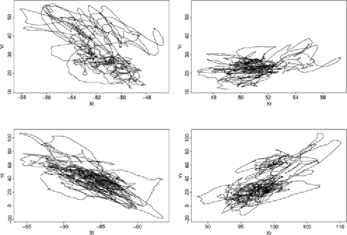
Figure 1 confirms the intuition that the structure of a generic trajectory $(X_{t})_{t\in T}$ is complicated, and that a mere visual inspection is, at least on this example, of little help for differentiating the normal and hemiplegic subjects. Although several articles investigate how to model and use such trajectories directly [Bertrand et al. (2001), Chambaz, Bonan and Vidal (2009)], we rather choose to rely on a summary measure of $(X_{t})_{t\in T}$ instead of relying on $(X_{t})_{t\in T}$.

2.2 Constructing a summary measure

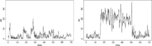
The summary measure that we construct is actually a summary measure of a one-dimensional trajectory $(C_{t})_{t\in T}$ that we initially derive from $(X_{t})_{t\in T}$. First, we introduce the trajectory of barycenters, $(B_{t})_{t\in T}=(\frac{1}{2}(L_{t}+R_{t}))_{t\in T}$. Second, we evaluate a reference position $b$ which is defined as the componentwise median value of $(B_{t})_{t\in T\cap[0,15]}$ (i.e., the median value over the first phase of the protocol). Third, we set $C_{t}=\|B_{t}-b\|_{2}$ for all $t\in T$, the Euclidean distance between $B_{t}$ and the reference position $b$, which provides a relevant description of the sway of the body during the course of the protocol. We plot in Figure 2 two examples of $(C_{t})_{t\in T}$ corresponding to two different protocols undergone by a hemiplegic subject.

Figure 2: Representing the trajectories $t\mapsto C_{t}$ over $T$ which correspond to two different protocols undergone by a hemiplegic subject (protocol 1 on the left, protocol 3 on the right).

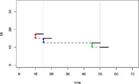
Because the most informative features can be found at the start and end of the second phase, we use the following finite-dimensional summary measure of $(X_{t})_{t\in T}$ [through $(C_{t})_{t\in T}$]:

$$Y=(\bar{C}_{1}^{+}-\bar{C}_{1}^{-},\bar{C}_{2}^{-}-\bar{C}_{1}^{+},\bar{C}_{2}^{+}-\bar{C}_{2}^{-}),$$ (1)

where

$$\bar{C}_{1}^{-} = \frac{\delta}{5}\sum_{t\in T\cap[10,15[}C_{t},\qquad\bar{C}_{1}^{+}=\frac{\delta}{5}\sum_{t\in T\cap\,]15,20]}C_{t},$$

$$\bar{C}_{2}^{-} = \frac{\delta}{5}\sum_{t\in T\cap[45,50[}C_{t},\qquad\bar{C}_{2}^{+}=\frac{\delta}{5}\sum_{t\in T\cap\,]50,55]}C_{t}$$

are the averages of $C_{t}$ computed over the intervals $[10,15[$, $]15,20]$, $[45,50[$ and $]50,55]$ (i.e., over the last/first 5 seconds before/after the beginning/ending of the second phase of the protocol of interest). We arbitrarily choose this 5-second threshold. Note that $\bar{C}_{2}^{-}-\bar{C}_{1}^{-}=Y_{2}+Y_{1}$, $\bar{C}_{2}^{+}-\bar{C}_{1}^{-}=Y_{3}+Y_{2}$, $\bar{C}_{2}^{+}-\bar{C}_{1}^{+}=Y_{1}+Y_{2}+Y_{3}$ are linear combinations of the components of $Y$. We refer to Figure 3 for a visual representation of the definition of the summary measure $Y$.

Figure 3: Visual representation of the definition of the finite-dimensional summary measure $Y$ of $(X_{t})_{t\in T}$. The four horizontal segments (solid lines) represent, from left to right, the averages $\bar{C}_{1}^{-}$, $\bar{C}_{1}^{+}$, $\bar{C}_{2}^{-}$, $\bar{C}_{2}^{+}$ of $(C_{t})_{t\in T}$ over the intervals $[10,15[$, $]15,20]$, $[45,50[$, $]50,55]$. The three vertical segments (solid lines ending by an arrow) represent, from top to bottom, the components $Y_{1}$, $Y_{2}$ and $Y_{3}$ of $Y$. Two additional vertical lines indicate the beginning and ending of the second phase of the considered protocol.

3 Classification procedure

We describe hereafter our two-step classification procedure. We formally introduce the statistical framework that we consider in Section 3.1. The first step of the classification procedure consists in ranking the protocols from the most to the less informative with respect to some criterion; see Section 3.2. The second step consists of the classification; see Section 3.3.

3.1 Statistical framework

The observed data structure $O$ writes as $O=(W,A,Y^{1},Y^{2},Y^{3},Y^{4})$, where

• $W\in\mathbb{R}\times\{0,1\}^{2}\times\mathbb{R}^{2}$ is the vector of baseline covariates (corresponding to initial age, gender, laterality, height and weight, see Section 2.1);

• $A\in\{0,1\}$ indicates the subject’s class (with convention $A=1$ for hemiplegic subjects and $A=0$ for normal subjects);

• for each $j\in\{1,2,3,4\}$, $Y^{j}\in\mathbb{R}^{3}$ is the summary measure [as defined in (1)] associated with the $j$th protocol.

We denote by $P_{0}$ the true distribution of $O$. Since we do not know much about $P_{0}$, we simply see it as an element of the nonparametric set $\mathcal{M}$ of all possible distributions of $O$.

We need a criterion to rank the four protocols from the most to the less informative in view of the subject’s class. To this end, we introduce the functional $\Psi\dvtx\mathcal{M}\to\mathbb{R}^{12}$ such that, for any $P\in\mathcal{M}$, $\Psi(P)=(\Psi^{j}(P))_{1\leq j\leq 4}$, where

$$\Psi^{j}(P)=(E_{P}\{E_{P}[Y_{i}^{j}|A=1,W]-E_{P}[Y_{i}^{j}|A=0,W]\})_{1\leq i\leq 3}.$$

The component $\Psi_{i}^{j}(P)$ is known in the literature as the variable importance measure of $A$ on the summary measure $Y_{i}^{j}$ controlling for $W$ [van der Laan and Rose (2011)]. Under causal assumptions, it can be interpreted as the effect of $A$ on $Y_{i}^{j}$. More generally, we are interested in $\Psi_{i}^{j}(P_{0})$ because the further it is from zero, the more knowledge on $A$ we expect to gain from the observation of $W$ and the summary measure $Y_{i}^{j}$ [i.e., by comparing the averages of $(C_{t})_{t\in T}$ computed over the time intervals corresponding to index $i$; see Section 2.2]. For instance, say that $\Psi_{1}^{2}(P_{0})>0$: this means that (in $P_{0}$-average) the variation in mean of the mean postures $\bar{C}_{1}^{-}$ and $\bar{C}_{1}^{+}$ of a hemiplegic subject computed before and after the beginning of the muscular perturbation is larger than that of a normal subject. In words, the postural control of a hemiplegic subject is more affected by the beginning of the muscular perturbation than the postural control of a normal subject.

3.2 Targeted maximum likelihood ranking of the protocols

Our ranking of the four protocols relies on testing the null hypotheses

$$\mbox{``}\Psi_{i}^{j}(P_{0})=0,\!\mbox{''}\qquad(i,j)\in\{1,2,3\}\times\{1,2,3,4\},$$

against their two-sided alternatives. Heuristically, rejecting “$\Psi_{i}^{j}(P_{0})=0$” tells us that the value of the $i$th coordinate of the summary measure $Y^{j}$ provides helpful information for the sake of determining whether $A=0$ or $A=1$.

We consider tests based on the targeted maximum likelihood methodology [van der Laan and Rubin (2006), van der Laan and Rose (2011)]. Because presenting a self-contained introduction to the methodology would significantly lengthen the article, we provide below only a very succinct description of it. The targeted maximum likelihood methodology relies on the super-learning procedure, a machine learning methodology for aggregating various estimators into a single better estimator [van der Laan, Polley and Hubbard (2007), van der Laan and Rose (2011)], based on the cross-validation principle. Since super-learning also plays a crucial role in our classification procedure (see Section 3.3), and because it is possible to present a relatively short self-contained introduction to the construction of a super-learner, we propose such an introduction in the supplementary file [Chambaz and Denis (2012)].

Let $O_{(1)},\ldots,O_{(n)}$ be $n$ independent copies of $O$. For each $(i,j)\in\{1,2,3\}\times\{1,2,3,4\}$, we compute the targeted maximum likelihood estimator (TMLE) $\Psi_{i,n}^{j}$ of $\Psi_{i}^{j}(P_{0})$ based on $O_{(1)},\ldots,O_{(n)}$ and an estimator $\sigma_{i,n}^{j}$ of its asymptotic standard deviation $\sigma_{i}^{j}(P_{0})$. The methodology applies because $\Psi_{i}^{j}$ is a “smooth” parameter. It notably involves the super-learning of the conditional means $Q_{i}^{j}(P_{0})(A,W)=E_{P_{0}}(Y_{i}^{j}|A,W)$ and of the conditional distribution $g(P_{0})(A|W)=P_{0}(A|W)$ (the collection of estimators aggregated by super-learning is given in the supplementary file [Chambaz and Denis (2012)]). Under some regularity conditions, the estimator $\Psi_{i,n}^{j}$ of $\Psi_{i}^{j}(P_{0})$ is consistent when either $Q_{i}^{j}(P_{0})$ or $g(P_{0})$ is consistently estimated, and it satisfies a central limit theorem. In addition, if $g(P_{0})$ is consistently estimated by a maximum-likelihood based estimator, then $\sigma_{i,n}^{j}$ is a conservative estimator of $\sigma_{i}^{j}(P_{0})$. Thus, we can consider in the sequel the test statistics $T_{i,n}^{j}=\sqrt{n}\Psi_{i,n}^{j}/\sigma_{i,n}^{j}$ (all $(i,j)\in\{1,2,3\}\times\{1,2,3,4\}$).

Now, we rank the four protocols by comparing the 3-dimensional vectors of test statistics $(T_{1,n}^{j},T_{2,n}^{j},T_{3,n}^{j})$ for $1\leq j\leq 4$. Several criteria for comparing the vectors were considered. They all relied on the fact that the larger is $|T_{i,n}^{j}|$ the less likely the null “$\Psi_{i}^{j}(P_{0})=0$” is true. Since the results were only slightly affected by the criterion, we focus here on a single one. Thus, we decide that protocol $j$ is more informative than protocol $j^{\prime}$ if

$$\sum_{i=1}^{3}(T_{i,n}^{j^{\prime}})^{2}<\sum_{i=1}^{3}(T_{i,n}^{j})^{2}.$$

This rule is motivated by the fact that, if $\sigma_{1,n}^{j}$, $\sigma_{2,n}^{j}$, $\sigma_{3,n}^{j}$ are consistent estimators of $\sigma_{1}^{j}(P_{0})$, $\sigma_{2}^{j}(P_{0})$, $\sigma_{3}^{j}(P_{0})$, then $\sum_{i=1}^{3}(T_{i,n}^{j})^{2}$ asymptotically follows the $\chi^{2}(3)$ distribution under $H_{0}^{j}\dvtx``\Psi^{j}(P_{0})=0$.”

By definition of $O$ and by construction of the TMLE procedure, this rule yields almost surely a final ranking of the four protocols from the more to the less informative for the sake of determining whether $A=0$ or $A=1$.

3.3 Classifying a new subject

We now build a classifier $\phi$ for determining whether $A=0$ or $A=1$ based on the baseline covariates $W$ and summary measures $(Y^{1},Y^{2},Y^{3},Y^{4})$. To study the influence of the ranking on the classification, we actually build four different classifiers $\phi^{1},\phi^{2},\phi^{3},\phi^{4}$ which, respectively, use only the best (more informative) protocol, the two best, the three best and all four protocols. So $\phi^{j}$ is a function of $W$ and of $j$ among the four vectors $Y^{1},Y^{2},Y^{3},Y^{4}$.

Say that $\mathcal{J}\subset\{1,2,3,4\}$ has $J$ elements. First, we build an estimator $h_{n}^{J}(W,Y^{j},j\in\mathcal{J})$ of $P_{0}(A=1|W,Y^{j},j\in\mathcal{J})$ based on $O_{(1)},\ldots,O_{(n)}$, relying again on the super-learning methodology (the collection of estimators involved in the super-learning is given in the supplementary file [Chambaz and Denis (2012)]). Second, we define

$$\phi^{J}(W,Y^{j},j\in\mathcal{J})=\mathbf{1}\bigl{\{}h_{n}(W,Y^{j},j\in\mathcal{J})\geq{\tfrac{1}{2}}\bigr{\}}$$

and decide to classify a new subject with information $(W,Y^{j},j\in\mathcal{J})$ into the group of hemiplegic subjects if $\phi^{J}(W,Y^{j},j\in\mathcal{J})=1$ or into the group of normal subjects otherwise.

Thus, the classifier $\phi^{J}$ relies on a plug-in rule, in the sense that the Bayes decision rule $\mathbf{1}\{P_{0}(A=1|W,Y^{j},j\in\mathcal{J})\geq{\frac{1}{2}}\}$ is mimicked by the empirical version where one substitutes an estimator of $P_{0}(A=1|W,Y^{j},j\in\mathcal{J})$ for the latter regression function. Such classifiers can converge with fast rates under a complexity assumption on the regression function and the so-called margin condition [Audibert and Tsybakov (2007)].

4 Simulation study

In this section we carry out and report the results of a simulation study of the performances of the classification procedure described in Section 3. The details of the simulation scheme are presented in Section 4.1, and the results are reported and evaluated in Section 4.2.

=280pt $\mbox{Scenario 1:}\operatorname{logit}g(P_{0}^{1})(A=1|W)=\displaystyle\frac{W_{1}}{50}+\frac{W_{2}}{50}-\frac{W_{3}}{10}-\frac{W_{4}}{2000}+W_{5}$ $\mbox{Scenario 2:}\operatorname{logit}g(P_{0}^{2})(A=1|W)=\cos(W_{1}+W_{5})+\sin(W_{1}+W_{5})$ $\mbox{Scenario 3:}\operatorname{logit}g(P_{0}^{3})(A=1|W)=\lfloor 10\cos(W_{1}+W_{3})\rfloor$ $\qquad{}+\displaystyle\sqrt{5\cos(W_{1}+W_{3})-\lfloor 5\cos(W_{1}+W_{3})\rfloor}\frac{\pi}{50}\sin\bigl{(}10\cos(W_{1}+W_{3})\bigr{)}$

Table 2: Characterization of the three conditional distributions $g(P_{0}^{k})$, $k=1,2,3,$ as considered in the simulation scheme

4.1 Simulation scheme

Instead of simulating $(W,A)$ and the four complex trajectories $(X_{t}^{1})_{t\in T}$, $(X_{t}^{2})_{t\in T}$, $(X_{t}^{3})_{t\in T}$, $(X_{t}^{4})_{t\in T}$ associated with four fictitious protocols, we generate directly $(W,A)$ and the summary measures $Y^{1}$, $Y^{2}$, $Y^{3}$, $Y^{4}$ that one would have derived from the trajectories $(X_{t}^{1})_{t\in T}$, $(X_{t}^{2})_{t\in T}$, $(X_{t}^{3})_{t\in T}$, $(X_{t}^{4})_{t\in T}$. Three different scenarios/probability distributions $P_{0}^{1},P_{0}^{2},P_{0}^{3}$ are considered. They only differ from each other with respect to the conditional distributions $g(P_{0}^{1})$, $g(P_{0}^{2})$, $g(P_{0}^{3})$ (see Table 2 for their characterization).

For each $k=1,2,3$, an observation $O=(W,A,Y^{1},Y^{2},Y^{3},Y^{4})$ drawnfrom $P_{0}^{k}$ meets the following constraints: [1.]

$W$ is drawn from a slightly perturbed version of the empirical distribution of $W$ as obtained from the original data set (the same for all $k=1,2,3$);

conditionally on $W$, $A$ is drawn from $g(P_{0}^{k})(\cdot|W)$;

conditionally on $(A,W)$ and for each $(i,j)\in\{1,2,3\}\times\{1,2,3,4\}$, $Y_{i}^{j}$ is drawn from the Gaussian distribution with mean $Q_{i}^{j}(A,W)$ (the same for all $k=1,2,3$; see Table 3 for the definition of the conditional means) and common standard deviation $\sigma\in\{0.5,1\}$.

Table 3: Conditional means $Q_{i}^{j}(A,W)$ of $Y_{i}^{j}$ given $(A,W)$, $(i,j)\in\{1,2,3\}\times\{1,2,3,4\}$, as used in the three different scenarios of the simulation scheme

Fictitious protocol	Conditional means
$j=1$	$\displaystyle Q_{1}^{1}(A,W)=2[A\sin(W_{1}+W_{4})+(1-A)\cos(W_{1}+W_{5})]$
	$\displaystyle Q_{2}^{1}(A,W)=3\biggl{[}(1-6A)X^{5}-AX^{4}+X^{3}-\biggl{(}1-\frac{A}{2}\biggr{)}X^{2}+AX\biggr{]}$
	$\hskip 143.0pt\displaystyle\mbox{where }X=\frac{(1-2A)W_{5}}{160}+\frac{A}{4}$
	$\displaystyle Q_{3}^{1}(A,W)=A\tan(W_{4})+(1-A)\tan(W_{5}+W_{1}W_{2})$
$j=2$	$\displaystyle Q_{1}^{2}(A,W)=\frac{1}{120}[A+W_{1}+W_{2}+W_{3}+W_{5}+W_{1}W_{2}$
	$\hskip 102.0pt\displaystyle{}+(1-A)W_{5}+W_{2}W_{3}W_{4}]$
	$\displaystyle Q_{2}^{2}(A,W)=5[A\sin(W_{1}+W_{4})+(1-A)\cos(W_{1}+W_{4})]$
	$\displaystyle Q_{3}^{2}(A,W)=\frac{1}{20}\biggl{[}A\biggl{(}2W_{1}+\frac{3}{2}W_{3}\biggr{)}+(1-A)W_{5}\biggr{]}$
$j=3$	$\displaystyle Q_{1}^{3}(A,W)=A\log\biggl{(}2W_{1}+\frac{3}{2}W_{3}\biggr{)}+(1-A)\log(W_{5})$
	$\displaystyle Q_{2}^{3}(A,W)=\frac{1}{45}(X+7)(X+2)(X-7)(X-3)$
	$\hskip 165.0pt\displaystyle\mbox{where }X=\frac{W_{4}+W_{5}}{145+AW_{1}}$
	$\displaystyle Q_{3}^{3}(A,W)=\pi\bigl{[}A\sin(X)\bigl{(}\lfloor 2X\rfloor+\sqrt{2X-\lfloor 2X\rfloor}\bigr{)}$
	$\hskip 56.0pt{}\displaystyle+(1-A)\cos(X)\bigl{(}\lfloor 2X\rfloor+\sqrt{2X-\lfloor 2X\rfloor}\bigr{)}\bigr{]}$
	$\hskip 135.0pt\displaystyle\mbox{where }X=\cos(W_{3}+W_{4}+W_{5})$
$j=4$	$\displaystyle Q_{1}^{4}(A,W)=\frac{1}{100}(2X^{3}+X^{2}-X-1)$
	$\hskip 144.0pt\displaystyle\mbox{where }X=\frac{AW_{2}+W_{4}+W_{5}}{30}$
	$\displaystyle Q_{2}^{4}(A,W)=\frac{1}{60}(A+W_{1}+W_{2}+W_{3}+W_{5})$
	$\displaystyle Q_{3}^{4}(A,W)=\frac{1}{1000}\biggl{[}\frac{W_{1}W_{3}W_{4}}{3}+(1-A)(W_{1}+W_{3}W_{4})+AW_{2}W_{5}\biggr{]}$

Figure 4: Visual representation of the three conditional distributions considered in the simulation scheme. We plot the empirical cumulative distribution functions of $\{g^{k}(A=1|W_{(\ell)})\dvtx\ell=1,\ldots,n\}$ for $k=1$ (solid line), $k=2$ (dashed line) and $k=3$ (dotted line), where $W_{(1)},\ldots,W_{(L)}$ are independent copies of $W$ drawn from the marginal distribution of $W$ under $P_{0}^{k}$ (which does not depend on $k$), and $L=10^{5}$.

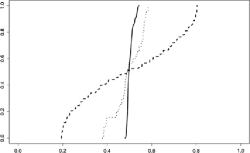
Although that may not be clear when looking at Table 2, the difficulty of the classification problem should vary from one scenario to the other. When using the first conditional distribution $g(P_{0}^{1})$, the conditional probability of $A=1$ given $W$ is concentrated around $\frac{1}{2}$, as seen in Figure 4 (solid line), with $P_{0}^{1}(g(P_{0}^{1})(1|W)\in[0.48,0.54])\simeq 1$. In words, the covariate provides little information for predicting the class $A$. On the contrary, estimating $g(P_{0}^{1})$ from the data is easy since $\operatorname{logit}g(P_{0}^{1})(A=1|W)$ is a simple linear function of $W$. The conditional probabilities of $A=1$ given $W$ under $g(P_{0}^{2})$ and $g(P_{0}^{3})$ are less concentrated around $\frac{1}{2}$, as seen in Figure 4 (dashed and dotted lines, resp.). Thus, the covariates may provide valuable information for predicting the class. But this time, $\operatorname{logit}g(P_{0}^{2})$ and $\operatorname{logit}g(P_{0}^{3})$ are tricky functions of $W$.

Likewise, the family of conditional means $Q_{i}^{j}(A,W)$ of $Y_{i}^{j}$ given $(A,W)$ that we use in the simulation scheme is meant to cover a variety of situations with regard to how difficult it is to estimate each of them and how much they tell about the class prediction. Instead of representing the latter conditional means, we find it more relevant to provide the reader with the values (computed by Monte-Carlo simulations) of

$$S^{j}(P_{0}^{k})=\sum_{i=1}^{3}\biggl{(}\frac{\Psi_{i}^{j}(P_{0}^{k})}{\sigma_{i}^{j}(P_{0}^{k})}\biggr{)}^{2}$$

for $(j,k)\in\{1,2,3,4\}\times\{1,2,3\}$ and $\sigma\in\{0.5,1\}$; see Table 4. Indeed, $nS^{j}(P_{0}^{k})$ should be interpreted as a theoretical counterpart to the criterion $\sum_{i=1}^{3}(T_{i,n}^{j})^{2}$. In particular, we derive from Table 4 the theoretical ranking of the protocols: for every scenario $P_{0}^{k}$ and $\sigma\in\{0.5,1\}$, the protocols ranked by decreasing order of informativeness are protocols 3, 2, 1, 4.

Table 4: Values of $S^{j}(P_{0}^{k})$ for $(j,k)\in\{1,2,3,4\}\times\{1,2,3\}$ and $\sigma\in\{0.5,1\}$. They notably teach us that, for every scenario $P_{0}^{k}$ and $\sigma\in\{0.5,1\}$, the protocols ranked by decreasing order of informativeness are protocols 3, 2, 1, 4

	Scenario 1		Scenario 2		Scenario 3
Fictitious protocol	$\bolds{\sigma=0.5}$	$\bolds{\sigma=1}$	$\bolds{\sigma=0.5}$	$\bolds{\sigma=1}$	$\bolds{\sigma=0.5}$	$\bolds{\sigma=1}$
$j=1$	0.14	0.04	0.11	0.03	0.14	0.04
$j=2$	0.86	0.37	0.74	0.31	0.85	0.37
$j=3$	2.94	1.12	2.49	0.93	2.90	1.11
$j=4$	0.06	0.01	0.04	0.01	0.06	0.01

4.2 Leave-one-out evaluation of the performances of the classification procedure

We rely on the leave-one-out rule to evaluate the performances of the classification procedure. We acknowledge that they usually result in overly optimistic error rates. Specifically, we repeat independently $B=100$ times the following steps for $k=1,2,3$: [1.]

Draw independently $O_{(1,b)},\ldots,O_{(n,b)}$ from $P_{0}^{k}$, with $n=54$; we denote by $A_{(\ell,b)}$ the group membership indicator associated with $O_{(\ell,b)}$, and by $O_{(\ell,b)}^{\prime}$ the observed data structure $O_{(\ell,b)}$ deprived of $A_{(\ell,b)}$.

For each $\ell\in\{1,\ldots,n\}$,

1. [(aaaaaaa)]

2. set $\mathcal{S}_{(\ell,b)}=\{O_{(\ell^{\prime},b)}\dvtx\ell^{\prime}\neq\ell,\ell^{\prime}\leq n\}$;

3. based on $\mathcal{S}_{(\ell,b)}$, rank the protocols (see Section 3.2), then build four classifiers $\phi^{1}_{(\ell,b)}$, $\phi^{2}_{(\ell,b)}$, $\phi^{3}_{(\ell,b)}$ and $\phi^{4}_{(\ell,b)}$ (see Section 3.3), which, respectively, use only the best (more informative), the two best, the three best and all four protocols (thus, $\phi^{J}_{(\ell,b)}$ is a function of the covariate $W$ and of $J$ among the four vectors $Y^{1}$, $Y^{2},Y^{3},Y^{4}$);

4. classify $O_{(\ell,b)}$ according to the four classifications $\phi^{1}_{(\ell,b)}(O_{(\ell,b)}^{\prime})$, $\phi^{2}_{(\ell,b)}(O_{(\ell,b)}^{\prime})$, $\phi^{3}_{(\ell,b)}(O_{(\ell,b)}^{\prime})$, $\phi^{4}_{(\ell,b)}(O_{(\ell,b)}^{\prime})$.

Compute $\operatorname{Perf}^{J}_{b}=\frac{1}{n}\sum_{\ell=1}^{n}\mathbf{1}\{A_{(\ell,b)}=\phi^{J}_{(\ell,b)}(O_{(\ell,b)}^{\prime})\}$ for $J=1,2,3,4$. From these results, we compute for each $J\in\{1,2,3,4\}$ the mean and standard deviation of the sample $(\operatorname{Perf}^{J}_{1},\ldots,\operatorname{Perf}^{J}_{B})$. All the standard deviations are approximately equal to 5%. Second, for every value of $\sigma\in\{0.5,1\}$, performance $\operatorname{Perf}^{J}$ actually depends only slightly on $J$ (i.e., on the number of protocols taken into account in the classification procedure), without any significant difference for $j=1,2,3,4$. Third, the latter performances all equal approximately 80% when $\sigma=1$, and increase to approximately 90% when $\sigma=0.5$. This increase is the expected illustration of the fact that the larger is the variability of the summary measures, the more difficult is the classification procedure. On the contrary, it is a little bit surprising that the conditional distributions $g(P_{0}^{1}),g(P_{0}^{2}),g(P_{0}^{3})$ do not affect significantly the performances. Anecdotally, the estimated ranking of the protocols always coincide with the ranking that we derived from Table 4.

5 Application to the real data set

We present here the results of the classification procedure of Section 3 applied to the real data set. Thus, we first rank the protocols from the more to the less informative regarding postural control (see Section 5.1); then we construct the four classifiers and rely on the leave-one-out rule to evaluate their performances (see Section 5.2). A natural extension of the classification procedure is considered and applied in Section 5.3, and yields significantly better results. We conclude the article with a discussion; see Section 5.4.

5.1 Targeted maximum likelihood ranking of the protocols over the real data set

Hemiplegic subjects are known to be sensitive to muscular stimulations, and also to tend to compensate for their proprioceptive deficit by developing a preference for visual information in order to maintain posture [Bonan et al. (1996)]. This suggests that protocols involving muscular and/or visual stimulations should rank high. What do the data tell us?

We derive and report in Table 5 the results of the ranking of the protocols using the entire data set. Table 5 teaches us that the most informative protocol is protocol 3 (visual and muscular stimulations), and that the three next protocols ranked by decreasing order of informativeness are protocols 2 (muscular stimulation), 1 (visual stimulation) and 4 (optokinetic stimulation). Apparently, protocols 3 and 2 (which have in common that muscular stimulations are involved) are highly relevant for differentiating normal and hemiplegic subjects based on postural control data. On the contrary (and perhaps surprisingly, given the introductory remark), protocols 1 and 4 seem to provide significantly less information for the same purpose.

Table 5: Ranking the four protocols using the entire real data set. We report the realizations of the criteria $\sum_{i=1}^{3}(T_{i,n}^{j})^{2}$ obtained for protocols $j=1,2,3,4$. These values teach us that the most informative protocol is protocol 3, and that the three next protocols ranked by decreasing order of informativeness are protocols 2, 1 and 4

Protocol	$\bolds{j=3}$	$\bolds{j=2}$	$\bolds{j=1}$	$\bolds{j=4}$
Criterion $\sum_{i=1}^{3}(T_{i,n}^{j})^{2}$	75.51	33.13	6.80	5.53

5.2 Classification procedures applied to the real data set

To evaluate the performances of the classification procedure applied to the real data set, we carry out steps 2a, 2b, 2c from the leave-one-out rule described in Section 4.2, where we substitute the real data set $O_{(1)},\ldots,O_{(n)}$ for the simulated one. We actually do it twice. The first time, the super-learning methodology involves a large collection of estimators; the second time, we justify resorting to a smaller collection (see the supplementary file [Chambaz and Denis (2012)]). We report the results in Table 6, where the second and third rows, respectively, correspond to the first (larger collection) and second (smaller collection) rounds of performance evaluation.

Consider first the performances of the classification procedure relying on the larger collection. The proportion of subjects correctly classified (evaluated by the leave-one-out rule) equals only 70% (38 out of the 54 subjects are correctly classified) when the sole most informative protocol (i.e., protocol 3) is exploited. This rate jumps to 80% (43 out of 54 subjects are correctly classified) when the two most informative protocols (i.e., protocols 3 and 2) are exploited. Including one or two of the remaining protocols decreases the performances.

Table 6: Leave-one-out performances $\operatorname{Perf}^{J}$ of the classification procedure using the real data set. Performance $\operatorname{Perf}^{J}$ corresponds to the classifier based on $J$ among the four vectors $Y^{1}$, $Y^{2},Y^{3},Y^{4}$ (those associated with the $J$ more informative protocols) and either using all estimators (second row) or only two of them (third row) in the super-learner (see Appendix A in the supplementary file [Chambaz and Denis (2012)])

	$\bolds{J=1}$	$\bolds{J=2}$	$\bolds{J=3}$	$\bolds{J=4}$
$\operatorname{Perf}^{J}$ (all est.)	0.70 (38/54)	0.80 (43/54)	0.74 (40/54)	0.78 (42/54)
$\operatorname{Perf}^{J}$ (two est.)	0.74 (40/54)	0.81 (44/54)	0.78 (42/54)	0.85 (46/54)

The theoretical properties of the super-learning procedure are asymptotic, that is, valid when the sample size $n$ is large, which is not the case in this study. Even though this is contradictory to the philosophy of the super-learning methodology, it is tempting to reduce the number of estimators involved in the super-learning. We therefore keep only two of them, and run again steps 2a, 2b, 2c from the leave-one-out rule described in Section 4.2, where we substitute the real data set $O_{(1)},\ldots,O_{(n)}$ for the simulated one. Results are reported in Table 6 (third row). We obtain better performances: for each value of $J$ (i.e., each number of protocols taken into account in the classification procedure), the second classifier outperforms the first one. The best performance is achieved when all four protocols are used, yielding a rate of correct classification equal to 85% (46 out of the 54 subjects are correctly classified). This is encouraging, notably because one can reasonably expect that performances will be improved on when a larger cohort is available.

Yet, this is not the end of the story. We have built a general methodology that can be easily extended, for instance, by enriching the small-dimensional summary measure derived from each complex trajectory. We explore the effects of such an extension in the next section.

5.3 Extension

Thus, we enrich the small-dimensional summary measure initially defined in Section 2.2. Since it mainly involves distances from a reference point, the most natural extension is to add information pertaining to orientation. Relying on polar coordinates of the trajectory $(B_{t})_{t\in T}$ poses some technical issues. Instead, we propose to fit simple linear models $y(B_{t})=vx(B_{t})+u$ [where $x(B_{t})$ and $y(B_{t})$ are the abscisse and ordinate of $B_{t}$] based on the data sets $\{B_{t}\dvtx t\in T\cap[10,15[\}$, $\{B_{t}\dvtx t\in T\cap[15,20[\}$, $\{B_{t}\dvtx t\in T\cap[20,45[\}$, $\{B_{t}\dvtx t\in T\cap[45,50[\}$ and $\{B_{t}\dvtx t\in T\cap[50,55[\}$, and to use the slope estimates as summary measures of an average orientation over each time interval. The observed data structure and parameter of interest still write as $O=(W,A,Y^{1},Y^{2},Y^{3},Y^{4})$ and $\Psi(P)=(\Psi^{j}(P))_{1\leq j\leq 4}$, but $Y^{j}$ and $\Psi^{j}(P)$ now belong to $\mathbb{R}^{8}$ (and not $\mathbb{R}^{3}$ anymore). The ranking of the protocols now relies on the criterion $\sum_{i=1}^{8}(T_{i,n}^{j})^{2}$, whose definition straightforwardly extends that of the criterion introduced in Section 3.2. The values of the criteria are reported in Table 7. The ranking of protocols remains unchanged, but the discrepancies between the values for protocol 2, on one hand, and for protocols 1 and 4, on the other hand, are smaller.

Table 7: Ranking the four protocols using the entire real data set and the extended small-dimensional summary measure of the complex trajectories. We report the realizations of the criteria $\sum_{i=1}^{8}(T_{i,n}^{j})^{2}$ obtained for protocols $j=1,2,3,4$. The ranking is the same as that derived from Table 5

Protocol	$\bolds{j=3}$	$\bolds{j=2}$	$\bolds{j=1}$	$\bolds{j=4}$
Criterion $\sum_{i=1}^{8}(T_{i,n}^{j})^{2}$	83.64	43.61	14.92	12.60

We finally apply once again steps 2a, 2b, 2c from the leave-one-out rule described in Section 4.2, where we substitute the real data set $O_{(1)},\ldots,O_{(n)}$ for the simulated one, and use either all estimators or only two of them in the super-learner. The results are reported in Table 8.

Table 8: Leave-one-out performances $\operatorname{Perf}^{J}$ of the classification procedure using the real data set and the extended small-dimensional summary measure of the complex trajectories. Performance $\operatorname{Perf}^{J}$ corresponds to the classifier based on $J$ among the four vectors $Y^{1}$, $Y^{2},Y^{3},Y^{4}$ (those associated with the $J$ more informative protocols) and either using all estimators (second row) or only two of them (third row) in the super-learner (see Appendix A in the supplementary file [Chambaz and Denis (2012)])

	$\bolds{J=1}$	$\bolds{J=2}$	$\bolds{J=3}$	$\bolds{J=4}$
$\operatorname{Perf}^{J}$ (all est.)	0.82 (44/54)	0.80 (43/54)	0.80 (43/54)	0.78 (42/54)
$\operatorname{Perf}^{J}$ (two est.)	0.87 (47/54)	0.85 (46/54)	0.80 (43/54)	0.82 (44/54)

When we include all estimators in the super-learner, the classification procedure that relies on the extended small-dimensional summary measure of the complex trajectories outperforms the classification procedure that relies on the initial summary measure, for every value of $J$ (i.e., each number of protocols taken into account in the classification procedure). The performances are even better when we only include two estimators. Remarkably, the best performance is achieved using only the most informative protocol, with a proportion of subjects correctly classified (evaluated by the leave-one-out rule) equal to 87% (47 out of the 54 subjects are correctly classified).

5.4 Discussion

We conducted a brief simulation study to evaluate the performances of the classification procedure. With its three different scenarios [i.e., three conditional distribution $g(P_{0}^{k})$] and four trajectories (i.e., twelve conditional means $Q_{i}^{j}$), the simulation scheme is far from comprehensive. Rather than extending the simulation study, we discuss here what additional scenarios would need to be considered before applying the procedure more generally. In the same spirit as in Section 4, one should consider the following:

• other conditional distributions $g(P_{0}^{k})$, $|g(P_{0}^{k}(A=1|W)-1/2|$ being close to 0 with high probability ($W$ strong predictor of $A$) or low probability ($W$ weak predictor of $A$);

• other conditional means $Q_{i}^{j}$, $(i,j)\in\{1,2,3\}\times\{1,2,3,4\}$, and standard deviation $\sigma$, $\{S^{j}(P_{0}^{k})\dvtx j=2,3,4\}$ having one, two, three or four well-separated values.

A straightforward generalization would consist in allowing the standard deviation of $Y_{i}^{j}$ to depend on $(i,j)$. Furthermore, another approach to simulating could be considered, where the trajectories $(X_{t}^{1})_{t\in T}$, $(X_{t}^{2})_{t\in T}$, $(X_{t}^{3})_{t\in T}$, $(X_{t}^{4})_{t\in T}$ would be obtained as realizations of stochastic processes satisfying a variety of piecewise stochastic differential equations (SDEs). For instance, the same SDE could be used to simulate the trajectory during the first and third phases ($0\to 15$ s and $50\to 70$ s, without perturbations), and another SDE could be used to simulate during the second phase ($15\to 50$ s, with perturbations). On top of that, the breaking points could be drawn randomly from two symmetric distributions centered at 15 s and 50 s.

This alternative approach to simulating arose while we were trying to quantify in some way how much information is lost when one substitutes a summary measure for the original trajectory for the purpose of classifying. Ultimately such a quantification could permit to elaborate new summary measures with minimal information loss. We did not obtain a satisfactory answer to this very difficult question. However, we identified important information that can be derived from the original trajectory, such as mean orientation, as used in Section 5.3, and empirical breaking points, as evoked for the sake of simulating in the previous paragraph, and used for the sake of classifying by Denis (2011).

References

- Audibert and Tsybakov (2007) {barticle}[mr] \bauthor\bsnmAudibert, \bfnmJean-Yves\binitsJ.-Y. and \bauthor\bsnmTsybakov, \bfnmAlexandre B.\binitsA. B. (\byear2007). \btitleFast learning rates for plug-in classifiers. \bjournalAnn. Statist. \bvolume35 \bpages608–633. \biddoi=10.1214/009053606000001217, issn=0090-5364, mr=2336861 \bptokimsref \endbibitem
- Bertrand et al. (2001) {barticle}[author] \bauthor\bsnmBertrand, \bfnmP.\binitsP., \bauthor\bsnmBardet, \bfnmJ-M.\binitsJ.-M., \bauthor\bsnmDabonneville, \bfnmM.\binitsM., \bauthor\bsnmMouzat, \bfnmA.\binitsA. and \bauthor\bsnmVaslin, \bfnmP.\binitsP. (\byear2001). \btitleAutomatic determination of the different control mechanisms in upright position by a wavelet method. \bjournalEngineering in Medicine and Biology Society, 2001. Proceedings of the 23rd Annual International Conference of the IEEE \bvolume2 \bpages1163–1166. \bptokimsref \endbibitem
- Bonan et al. (1996) {barticle}[author] \bauthor\bsnmBonan, \bfnmI.\binitsI., \bauthor\bsnmYelnik, \bfnmA.\binitsA., \bauthor\bsnmLaffont, \bfnmI.\binitsI., \bauthor\bsnmVitte, \bfnmE.\binitsE. and \bauthor\bsnmFreyss, \bfnmG.\binitsG. (\byear1996). \btitleSelection of sensory information in postural control of hemiplegics after unique stroke. \bjournalAnnales de Réadaptation et de Médecine Physique \bvolume39 \bpages157–163. \bptokimsref \endbibitem
- Chambaz and Denis (2012) {bmisc}[mr] \bauthor\bsnmChambaz, \bfnmAntoine\binitsA. and \bauthor\bsnmDenis, \bfnmChristophe\binitsC. (\byear2012). \bhowpublishedSupplement to “Classification in postural style.” DOI:\doiurl10.1214/12-AOAS542SUPP. \bptokimsref \endbibitem
- Chambaz, Bonan and Vidal (2009) {barticle}[mr] \bauthor\bsnmChambaz, \bfnmAntoine\binitsA., \bauthor\bsnmBonan, \bfnmIsabelle\binitsI. and \bauthor\bsnmVidal, \bfnmPierre-Paul\binitsP.-P. (\byear2009). \btitleDeux modèles de Markov caché pour processus multiples et leur contribution à l’élaboration d’une notion de style postural. \bjournalJ. SFdS \bvolume150 \bpages73–100. \bidissn=2102-6238, mr=2609698 \bptokimsref \endbibitem
- Denis (2011) {bmisc}[author] \bauthor\bsnmDenis, \bfnmC.\binitsC. (\byear2011). \bhowpublishedClassification in postural maintenance based on stochastic process modeling. Prépublication MAP5_2011-34, référence HAL hal-00653316. \bptokimsref \endbibitem
- Newell et al. (1997) {barticle}[author] \bauthor\bsnmNewell, \bfnmK. M.\binitsK. M., \bauthor\bsnmSlobounov, \bfnmS. M.\binitsS. M., \bauthor\bsnmSlobounova, \bfnmE. S.\binitsE. S. and \bauthor\bsnmMolenaar, \bfnmP. C. M.\binitsP. C. M. (\byear1997). \btitleStochastic processes in postural center-of-pressure profiles. \bjournalExperimental Brain Research \bvolume113 \bpages158–164. \bptokimsref \endbibitem
- van der Laan, Polley and Hubbard (2007) {barticle}[mr] \bauthor\bparticlevan der \bsnmLaan, \bfnmMark J.\binitsM. J., \bauthor\bsnmPolley, \bfnmEric C.\binitsE. C. and \bauthor\bsnmHubbard, \bfnmAlan E.\binitsA. E. (\byear2007). \btitleSuper learner. \bjournalStat. Appl. Genet. Mol. Biol. \bvolume6 \bpagesArt. 25, 23 pp. (electronic). \biddoi=10.2202/1544-6115.1309, issn=1544-6115, mr=2349918 \bptokimsref \endbibitem
- van der Laan and Rose (2011) {bbook}[author] \beditor\bparticlevan der \bsnmLaan, \bfnmM. J.\binitsM. J. and \beditor\bsnmRose, \bfnmS.\binitsS., eds. (\byear2011). \btitleTargeted Learning: Causal Inference for Observational and Experimental Data. \bpublisherSpringer, \baddressNew York. \bidmr=2867111 \bptokimsref \endbibitem
- van der Laan and Rubin (2006) {barticle}[mr] \bauthor\bparticlevan der \bsnmLaan, \bfnmMark J.\binitsM. J. and \bauthor\bsnmRubin, \bfnmDaniel\binitsD. (\byear2006). \btitleTargeted maximum likelihood learning. \bjournalInt. J. Biostat. \bvolume2 \bpagesArt. 11, 40. \biddoi=10.2202/1557-4679.1043, issn=1557-4679, mr=2306500 \bptokimsref \endbibitem