Fitting functions for dark matter density profiles

Abstract

We present a unified parameterization of the fitting functions suitable for density profiles of dark matter haloes or elliptical galaxies. A notable feature is that the classical Einasto profile appears naturally as the continuous limiting case of the cored subfamily amongst the double power-law profiles of Zhao. Based on this, we also argue that there is basically no qualitative difference between halo models well-fitted by the Einasto profile and the standard NFW model. This may even be the case quantitatively unless the resolutions of simulations and the precisions of fittings are sufficiently high to make meaningful distinction possible.

1 Introduction

Although it is often claimed that the density profiles of dark matter haloes found in simulations are well described by simple double power-law functions of radii (see e.g., Navarro, Frenk & White, 1995, henceforth NFW), these are usually based on the fitting with limited radial coverage. A possible manifestation of this limitation is that these functions, when they are extrapolated to the centre, typically possess a singularity, which is generally unphysical. Real dynamical systems almost certainly have finite phase-space densities, finite number densities, and finite escape speeds even at the centre, as argued by fundamental physics: (1) any halo with fermions are limited in phase-space density by the Pauli exclusion principle; (2) any annihilating dark matter particle is limited in the number density by the annihilation cross section; (3) any stellar system is limited by its relaxation time; and (4) the escape speed is limited at least by the speed of light. To ameliorate the singularity whilst introducing the fewest extra parameters is to make the density profile more flexible in its parameterization.

In fact, the results from more recent high resolution simulations (see e.g., Navarro et al., 2010) appear to suggest that a different class of fitting formula such as that of Einasto (1965, 1969) introduced earlier for spherical stellar systems may be more close to the ‘reality’. The Einasto profiles by construction have finite densities, but they are less user friendly given their exponential behaviours. This motivates us to look for smooth transitions from double power laws to the Einasto models. Although they seem to be qualitatively different at first glance, the fitting formulae for the double power laws and the Einasto profiles are indeed closely related. For example, the Gaussian and the Plummer profile are limiting cases of the so-called beta profile for hot X-ray gas haloes, $\propto(1+r^{2}/a^{2})^{-(\beta+1/2)}$ for $\beta\rightarrow\infty$ or $\beta=2$ respectively. This hints to us that it may also be possible to connect the entire family of double power laws and the Einasto profiles. We shall show that this is achieved by simply redefining parameters of the double power-law models. This is also analogous to relating an isothermal sphere to polytropic models as in the infinite-index power law reducing to an exponential.

We argue that this connection is more than a mere mathematical trick, for it suggests that a cored double power-law profile with a large outer power-index value and the Einasto profile should be qualitatively indistinguishable if the fitting is mostly weighted near and around the central regions. Moreover, the resolution limit indicates that the fittings to dark halo profiles, be they numerical simulations or some observational proxies, are mostly concerned with the behaviour around the ‘scale radius’, that is, corresponding to the transition regions in the model. Hence, combined with the uncertainties in the fittings, it is expected that most cusped double power-law profiles with a moderate outer slope, such as the NFW profile and the Hernquist (1990) model, may not be well-distinguished from some cored profiles with an extreme value of the outer slope or even exponential fall-off if the variations of the logarithmic slope in the latter models are made to be sufficiently slower than the former. Here we shall show that, in the context of our extended family of models, this is indeed the case.

Despite widespread use of the double power-law profile, this possibility has not been investigated in detail, for in practice most focus on the double power law has been limited to the two limiting power indices and scarce attention has been paid to the parameter controlling the sharpness of the transition. The connection of the double power-law profiles to the Einasto profile, for which the variation of the shape parameter has received more attention, thus also highlights the role of the corresponding parameter in the double power law, and subsequently the above-mentioned difficulty of distinguishing fitting functions.

Figure 1: Density profiles of selected members of the family. All models drawn have $\alpha=1$ and $p=1$ but the values of the parameter $s$ vary with $\delta=3,4,5,9,15$ and $s=0$, where $\delta=s^{-1}$. The models with $(\alpha,\delta,p)=(1,3,1)$ and $(\alpha,\delta,p)=(1,4,1)$ correspond to the so-called NFW profile and Hernquist model, respectively. In the top panel, the plots are normalized for a fixed $\varrho_{\mathrm{s}}$ and $r_{\mathrm{s}}$ whilst they are for $\varrho_{-2}$ and $r_{-2}$ in the bottom panel. In addition, in the bottom panel, they are further scaled by $r^{-2}$ so that the horizontal tangent in the figure indicates that local power index of ${-2}$.

Figure 2: Same as Fig. 1 but with different members of the family with varying $p$. Again all models shown have $r^{-1}$ cusp ($\alpha=1$) but only those with two different outer slopes, $\delta=3$ (drawn in thick lines) and an exponential fall-off ($s=0$; thin lines) are chosen. Varying $p$ values are indicated by different line types: dashed ($p=2$), solid ($p=1$), dot-dashed ($p=\frac{1}{2}$), and dotted ($p=\frac{1}{4}$).

2 fitting formulae for density profiles

2.1 The Double power law

A widely-used fitting formula for the density profiles of the dark haloes found in cosmological simulations is of the form of a ‘broken’ or double power-law profile (Hernquist, 1990; Zhao, 1996):

$$\varrho(r)\propto\frac{a^{\delta}}{r^{\alpha}(a^{p}+r^{p})^{(\delta-\alpha)/p}}\,;\qquad\frac{\mathrm{d}\log\varrho}{\mathrm{d}\log r}=-\frac{\alpha a^{p}+\delta r^{p}}{a^{p}+r^{p}}.$$ (1)

Here, the parameters $\alpha<3$ and $\delta$ correspond to the power indices of the density profile at the centre and towards the asymptotic limit. By considering only such profiles with vanishing density at infinity, with possibility of escape (i.e., the potential at infinity can be set to a finite value), or with a finite total mass, allowed values of the parameter $\delta$ may be restricted to be $\delta>0$, $\delta>2$, or $\delta>3$. The parameter $p>0$ controls the width of the transition region between the two limiting behaviours; that is, the transition becomes sharper as $p$ gets larger. Finally, the scale length $a$ in equation (1) specifies the radius at which the local logarithmic density slope is the same as the arithmetic mean of the two limiting values.

The well-known special cases of these models include: the Schuster (1884)–Plummer (1911) sphere ($\alpha=0$, $\delta=5$, $p=2$: an index-5 polytrope); the Jaffe (1983) model ($\alpha=2$, $\delta=4$, $p=1$); the Hernquist (1990) model ($\alpha=1$, $\delta=4$, $p=1$); the NFW profile ($\alpha=1$, $\delta=3$, $p=1$); and the isotropic analytic solution of Austin et al. (2005) and Dehnen & McLaughlin (2005) ($\alpha=\frac{7}{9}$, $\delta=\frac{31}{9}$, $p=\frac{4}{9}$). Also notable are the families of models: the $\gamma$-sphere studied by Dehnen (1993) and Tremaine et al. (1994) ($\delta=4$, $p=1$); the generalized NFW profiles of Navarro et al. (1996, 1997) ($\delta=3$, $p=1$); the $\beta$-sphere of Zhao (1996) ($\alpha=1$, $p=1$: which corresponds to alternative generalized NFW profiles studied by Evans & An 2006); the hypervirial family of Evans & An (2005) ($\alpha=2-p$, $\delta=p+3$: which was originally introduced as the generalized isochronous model by Veltmann 1979); and the phase-space power-law solutions of Dehnen & McLaughlin (2005) ($\alpha=1-\frac{p}{2}+\beta_{0}$, $\delta=3+p$: where $\beta_{0}$ is the anisotropy parameter at the centre).

2.2 The Einasto profile

Navarro et al. (2004) introduced a different class of fitting formulae for the density profile of dark haloes, namely,

$$\varrho\propto\exp\!\left\lgroup-\eta\,\frac{r^{p}}{a^{p}}\right\rgroup\,;\qquad\frac{\mathrm{d}\log\varrho}{\mathrm{d}\log r}=-p\eta\,\frac{r^{p}}{a^{p}}.$$ (2)

Here $p$ is the parameter controlling how rapidly the logarithmic density slope varies. Note the $p=2$ case corresponds to the isotropic Gaussian. The choices of the scale length $a$ and the constant $\eta$ are not independent but the physical definition of one specifies the other. For example, if $a=r_{-2}$ where $r_{-2}$ is the radius at which the logarithmic density slope is ‘$-2$’, then $\eta=\frac{2}{p}$. This family is usually referred to as the Einasto profile after Einasto (1965, 1969). It also has the same form as the fitting function proposed by Sérsic (1968) and de Vaucouleurs (1948) (the latter is a particular case of the former), which have been used to fit the surface brightness profile of elliptical (or spheroidal components of) galaxies (Merritt et al., 2005).

Figure 3: Rotation curve for select models; NFW profile ($\alpha=1$, $\delta=3$, $p=1$; solid lines), the Hernquist model ($\alpha=2$, $\delta=4$, $p=1$; dashed lines), Schuster-Plummer sphere ($\alpha=0$, $\delta=5$, $p=2$; dotted lines), $r^{-1}$ cusped exponential fall-off ($\alpha=1$, $s=0$, $p=1$; dot-dashed lines), and Sérsic-Einasto profile with $p=\frac{1}{2}$ ($\alpha=0$, $s=0$, $p=\frac{1}{2}$). The plots are normalized to have the same circular speed at $r=r_{-2}$. Among the models shown, only the NFW profile has an infinite total mass. All remaining models have a finite total mass and so their circular speed speeds fall off as $1/\sqrt{r}$.

3 An Extension of The Double Power Law

Functions used to fit the logarithmic density slope in equations (1) and (2) are first-order rational functions of $r^{p}$. Here we consider a slight variant version of equation (1) given by

$$\frac{\mathrm{d}\log\varrho}{\mathrm{d}\log r}=-\frac{\alpha r_{\mathrm{s}}^{p}+r^{p}}{r_{\mathrm{s}}^{p}+sr^{p}}.$$ (3)

This is actually the most general first-order monomial rational function of $r^{p}$ encompassing both equations (1) and (2) that may be used to fit any physical profile of the logarithm density slope. Here we assume $r_{\mathrm{s}}>0$ without any loss of generality (the $r_{\mathrm{s}}=0$ case corresponds to a pure power law, which may be described by other parameter combinations). This reduces to equation (1) through the parameter transformation $\delta=s^{-1}$ and $a^{p}=\delta r_{\mathrm{s}}^{p}$, but it now includes the models with $s=0$ (i.e., $\delta=\infty$) in places of those with $\delta=0$, which would represent unphysical asymptotically non-vanishing density profiles. The $(\alpha,s)=(0,0)$ models correspond to those of equation (2) with $a^{p}=p\eta r_{\mathrm{s}}^{p}$. That is to say, equation (1) with $\alpha=0$ (a cored double power law) reduces to equation (2) by taking the limit of $\delta\rightarrow\infty$ and $a\rightarrow\infty$ whilst maintaining $a^{p}/\delta=r_{\mathrm{s}}^{p}$ constant (and redefining $a^{p}=p\eta r_{\mathrm{s}}^{p}$ afterwards).

In equation (3), the parameter $\alpha<3$ still specifies the central power index whereas $s>0$ is now the reciprocal of the asymptotic index. The limits for the finite total mass, the escapability, and the well-defined integrated density along any line of sight are given respectively by $0\leq s<\frac{1}{3}$, $0\leq s<\frac{1}{2}$, and $0\leq s<1$. We may introduce a further restriction $s<\alpha^{-1}$ by limiting ourselves to models whose outer logarithmic slope is steeper than the inner value. The parameter $p>0$ again controls the steepness of the index variation and the breadth of the transition region. On the other hand, although the parameter $r_{\mathrm{s}}$ still specifies the nominal scale length, it lacks any immediate physical interpretation. By allowing an infinite asymptotic power index, the arithmetic mean of the limiting indices is not necessarily defined (note the scale length defined as eq. 1 becomes infinite). An alternative physical scale length may be defined such as the radius at which the local logarithmic slope is the same as a given fixed value, e.g.,

$$r_{-n}^{p}=\frac{n-\alpha}{1-ns}\,r_{\mathrm{s}}^{p}=\frac{n-\alpha}{\delta-n}\,\delta\,r_{\mathrm{s}}^{p}.$$ (4)

Here the corresponding logarithmic slope is $(-n)<0$. This is defined for the models for $\alpha<n$ and $s<n^{-1}$, and simplifies, if $s=0$, to $r_{-n}^{p}=(n-\alpha)r_{\mathrm{s}}^{p}$. The most common choice for the reference logarithmic slope is $(-n)=(-2)$, which corresponds to that of a singular isothermal sphere.

3.1 Density profiles

The actual functional form of the density profile is obtained by integrating equation (3). If $s>0$, this results in

$$\begin{split}\varrho(r)&=\varrho_{\mathrm{s}}\,(1+s)^{\frac{\delta-\alpha}{p}}\frac{r_{\mathrm{s}}^{\alpha}}{r^{\alpha}}\left(1+\frac{r^{p}}{\delta\,r_{\mathrm{s}}^{p}}\right)^{-\frac{\delta-\alpha}{p}}\\ &=\varrho_{-2}\left(\frac{\delta-\alpha}{\delta-2}\right)^{\frac{\delta-\alpha}{p}}\left(\frac{r_{-2}}{r}\right)^{\alpha}\left[1+\frac{2-\alpha}{\delta-2}\left(\frac{r}{r_{-2}}\right)^{p}\right]^{-\frac{\delta-\alpha}{p}},\end{split}$$ (5a)

which reproduces the double power-law profile (we have used the substitution $$\delta=s^{-1}>0 \varrho(r_{\mathrm{s}})=\varrho_{\mathrm{s}} \varrho(r_{-2})=\varrho_{-2}$$ for clarity). The integration also introduces an additional constant of integration, namely, the scale constant. We have chosen this scale constant in reference to the scale length, that is, and . The relation between them is

$$\left(\frac{\varrho_{-2}}{\varrho_{\mathrm{s}}}\right)^{p}=\frac{(1-2s)^{\delta}}{(2-\alpha)^{\alpha}}\,\left(\frac{1+\delta}{\delta-\alpha}\right)^{\delta-\alpha}.$$ (5b)

We also use $\bar{\varrho}_{\mathrm{s}}\equiv(1+s)^{(\delta-\alpha)/p}\varrho_{\mathrm{s}}$, which is useful for compactly writing down many properties of haloes. This is also related to the proportionality constant of the usual expression of the double power law in equation (1) such that $C=\bar{\varrho}a^{\alpha}=\bar{\varrho}_{\mathrm{s}}r_{\mathrm{s}}^{\alpha}$ given $a^{p}=\delta r_{\mathrm{s}}^{p}$.

With $s=0$, the integration leads to the density profile given by

$$\begin{split}\varrho(r)&=\varrho_{\mathrm{s}}\,\mathrm{e}^{1/p}\frac{r_{\mathrm{s}}^{\alpha}}{r^{\alpha}}\exp\!\left\lgroup-\frac{r^{p}}{pr_{\mathrm{s}}^{p}}\right\rgroup\\ &=\varrho_{-2}\,\left(\frac{r_{-2}}{r}\right)^{\alpha}\exp\!\left\lgroup-\frac{2-\alpha}{p}\left[\left(\frac{r}{r_{-2}}\right)^{p}-1\right]\right\rgroup,\end{split}$$ (6a)

and the scale constants related by

$$\left(\frac{\varrho_{-2}}{\varrho_{\mathrm{s}}}\right)^{p}=\frac{\mathrm{e}^{\alpha-1}}{(2-\alpha)^{\alpha}}.$$ (6b)

We also define $\bar{\varrho}_{\mathrm{s}}\equiv\mathrm{e}^{1/p}\varrho_{\mathrm{s}}$, which is the limit of the prior definition as $s\rightarrow 0$. The transition of models from $s>0$ to $s=0$ is also smooth – equation (6a) is indeed the limit of equation (5a) as $s\rightarrow 0$ ($\delta\rightarrow\infty$). The profile in equation (6a) is a generalization of the Einasto profile of equation (2) allowing a central density cusp. The classical profile consists of the cored members ($\alpha=0$) of the family with the index $n=p^{-1}$ whilst a cusped model ($\alpha=-1.85$) has been recently used to model the Galactic spheroid (Wang et al., 2012).

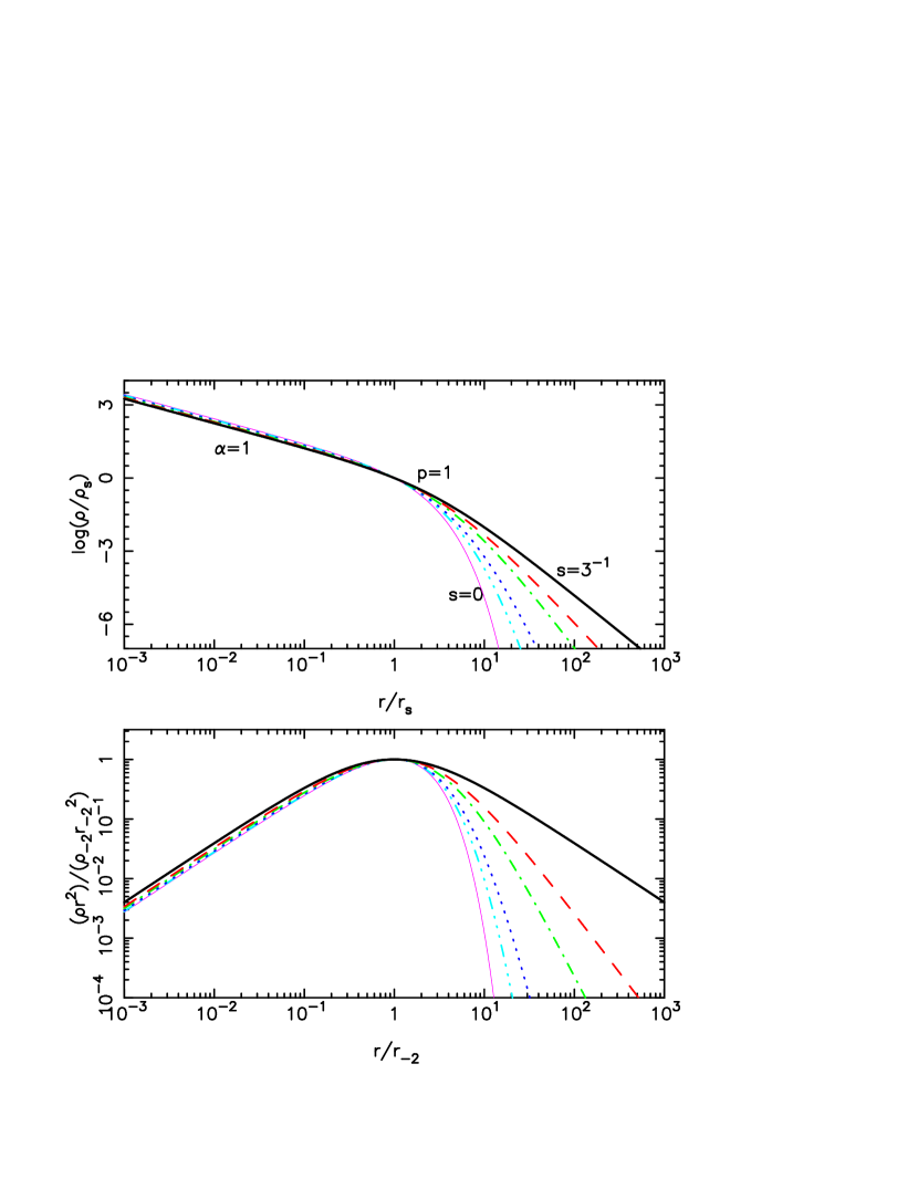
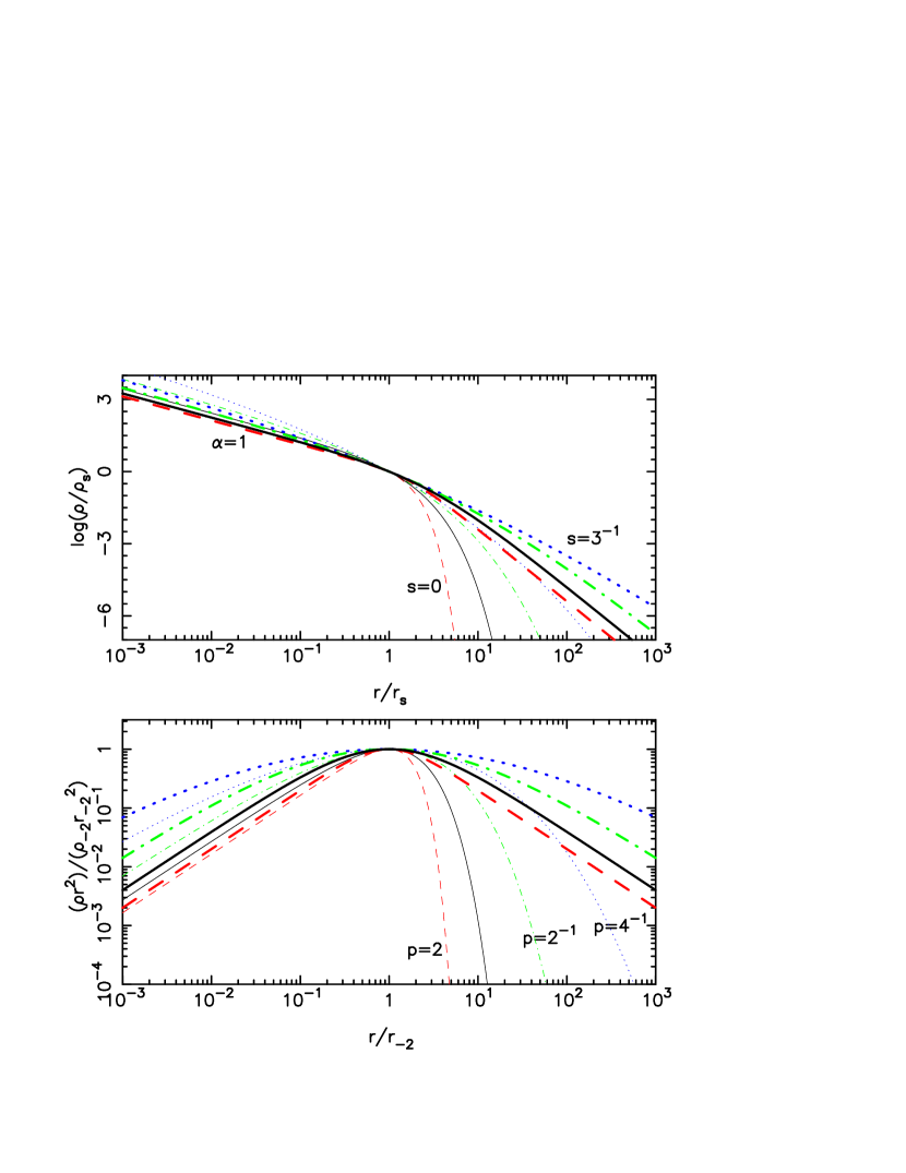
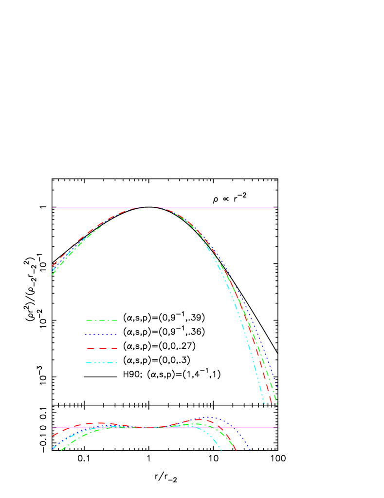
Figures 1 and 2 present the log-log plots of density profiles for select members of the family. Here the shape of the profiles is fixed by three of the parameters $(\alpha,s=\delta^{-1},p)$, whereas varying the scale length or constant simply translates the graph horizontally (for the scale length) or vertically (for the scale constant). Figure 1 demonstrates that the transition of an extreme power law to an exponential fall-off is indeed natural. The role of parameter $p$ as characterizing the breath of the transition region is highlighted in Figure 2.

Figure 4: Energy part of the distribution function (upper panel) and the differential energy distribution (lower panel) of the constant-anisotropy Hernquist model with a black hole for $\beta=\frac{1}{2}$ (left) and $\beta=-\frac{1}{2}$ (right): thin solid lines (no black hole), thick dotted lines ($M_{\bullet}=M_{\mathrm{tot}}/100$), thick solid lines ($M_{\bullet}=M_{\mathrm{tot}}/10$), thin dotted lines ($M_{\bullet}=M_{\mathrm{tot}}/2$), short-dashed lines ($M_{\bullet}=M_{\mathrm{tot}}$), long-dashed lines ($M_{\bullet}=3M_{\mathrm{tot}}/2$), dot-dashed lines ($M_{\bullet}=2M_{\mathrm{tot}}$) where $M_{\mathrm{tot}}$ is the total dark halo mass. All models are normalized to the same $M_{\mathrm{tot}}$. Note $0\leq\mathcal{E}\leq GM_{\mathrm{tot}}/a$ when there is no black hole whereas $\mathcal{E}\geq 0$ otherwise.

3.2 Basic properties

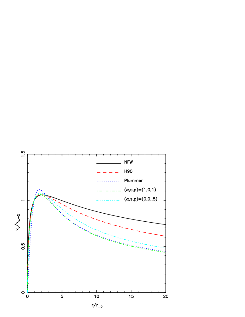
Deriving basic properties of these models such as the enclosed mass profiles $M_{r}$, the rotation curves (i.e., the circular speed) $\varv_{\mathrm{c}}$, the potential $\psi$ etc. is basically an exercise in integration. These integrals are trivial to evaluate numerically and usually result in special functions of radii no more complicated than beta and gamma functions. We refer Appendix A for more systematic studies, which may be of some peripheral interest. Here instead we simply provide the rotation curves for some familiar models and those with exponential fall-off in Figure 3. Since the total mass is finite for $\delta>3$, the circular speeds for all plotted models fall off as Keplerian – i.e., $\varv_{\mathrm{c}}^{2}\in\varTheta(r^{-1})$ – for large enough radii, except for the NFW profile, whose mass profile grows logarithmically and thus $\varv_{\mathrm{c}}^{2}$ falls off like $r^{-1}\ln r$. For models with $\delta<3$, it is obvious that the circular speed would behave like $\varv_{\mathrm{c}}^{2}\in\varTheta(r^{2-\delta})$ as $r\rightarrow\infty$. None of the plotted models possesses a cusp diverging faster or as fast as that of a singular isothermal sphere. Hence $\varv_{\mathrm{c}}^{2}\in\varTheta(r^{2-\alpha})$ and so $\varv_{\mathrm{c}}^{2}\rightarrow 0$ as $r\rightarrow 0$ in Figure 3. If $\alpha<2<\delta$ like those plotted, $\varv_{\mathrm{c}}$ attains its maximum at the radius corresponding to the solution of $M_{r}=4\pi r^{3}\varrho(r)$ (i.e., $\mathrm{d}\log M_{r}/\mathrm{d}\log r=1$). This occurs around $r\approx r_{-2}$ for the models plotted in Figure 3. Either if $\delta$ is not so much different from the nominal value of ‘${-2}$’ or if the profile has an extended transition region (achieved by small $p$), the variation of $\varv_{\mathrm{c}}$ then become sufficiently slow so that the behaviour of the circular speed can mimic the flat rotation curve near the region around $r\approx r_{-2}$.

We also find that $M_{r}\in\varTheta(r^{3-\alpha})$ as $r\rightarrow 0$ for $\alpha<3$, which is obvious from the fact that $\mathrm{d}M_{r}/\mathrm{d}r=4\pi r^{2}\varrho\in\varTheta(r^{2-\alpha})$ as $r\rightarrow 0$ (assuming the null integration constant). Realistically, any model with $2<\alpha<3$ cannot be strictly physical extending down all the way to the centre, for the corresponding $M_{r}\in\varTheta(r^{3-\alpha})$ would imply that there must exist a radius below which $r\leq 2GM_{r}c^{-2}$. This would lead to a gravitational collapse to a singularity and necessarily a central black hole (or at least the relativistic effects must be considered for proper understanding). If the particle dark matter are indeed cold, the origin of the pressure support is crucial to understand any presence of the density cusp or core. If the cold dark matter (CDM hereafter) halo consists of fermions, then the quantum mechanical effects, in particular, the maximum phase-space density is limited by the mass of the particles (i.e., ${\rm df}_{\max}\propto m_{\mathrm{f}}^{4}$) and the consequent degenerate pressure may play a role before the relativistic effects do. In this regard, it is of special interest to study models with a finite central density (see Sect. 4.1) which generally have a finite phase-space density at the centre too, if dark haloes are limited by the degenerate pressure of fermions.

3.3 Dynamical properties

Assessing the dynamical properties associated with these models typically requires additional assumptions e.g., regarding the velocity anisotropy etc. Some of these are straightforward: for instance, under the ergodic distribution assumption, the unique self-consistent distribution may be found by means of the Eddington (1916) formula although usually the tasks are more involved and in general the results are somewhat cumbersome. The reader is again referred to Appendix B for more systematic studies. Here we just note that the Hernquist (1990) model in this regard is the most special (cf., Baes & Dejonghe, 2002), for a quite a few complete analytically-tractable dynamical models of the Hernquist profile are known. In Figure 4 for example, we present the distribution function and the differential energy distribution with the constant anisotropy given by $\beta=\frac{1}{2},-\frac{1}{2}$ for the dark halo of the Hernquist profile with a central black hole (see Appendix B.2.3 for details).

Figure 5: Density plots of select cored halo models, compared to the NFW profile (top) and the Hernquist model (bottom).

4 The cusp/core problem and densities in projection

We now turn to comparisons of these models with simulated haloes, and consider them in the context of the core/cusp problem.

4.1 A Family of cored profiles

Whilst earlier N-body simulations seemed to suggest that CDM haloes follow the universal density profile with a central density cusp, emerging evidence from recent high resolution simulations indicate that those findings may have resulted from insufficient resolving power of earlier simulations. Newer simulations such as the Aquaris Project (Springel et al., 2008) that better resolve the central behaviours show continually varying logarithmic density slopes (claimed to be well fit by the Einasto profile). We have shown that the Einasto profiles are an extension of the double power law to a member with a central core and an exponential fall-off. With a sufficiently slow transition and the consequently broad transition zone, continually varying logarithmic density slopes are not necessarily inconsistent with the presence of a central core, given the difficulty of simulating and resolving the central region of dark haloes. Despite the lack of nominal thermal pressure support, there are some theoretical arguments, such as the degenerate pressure of fermion ‘gas’ that argue for a core at the centre of each CDM halo. All these shepherd us to study the cored members amongst our model family.

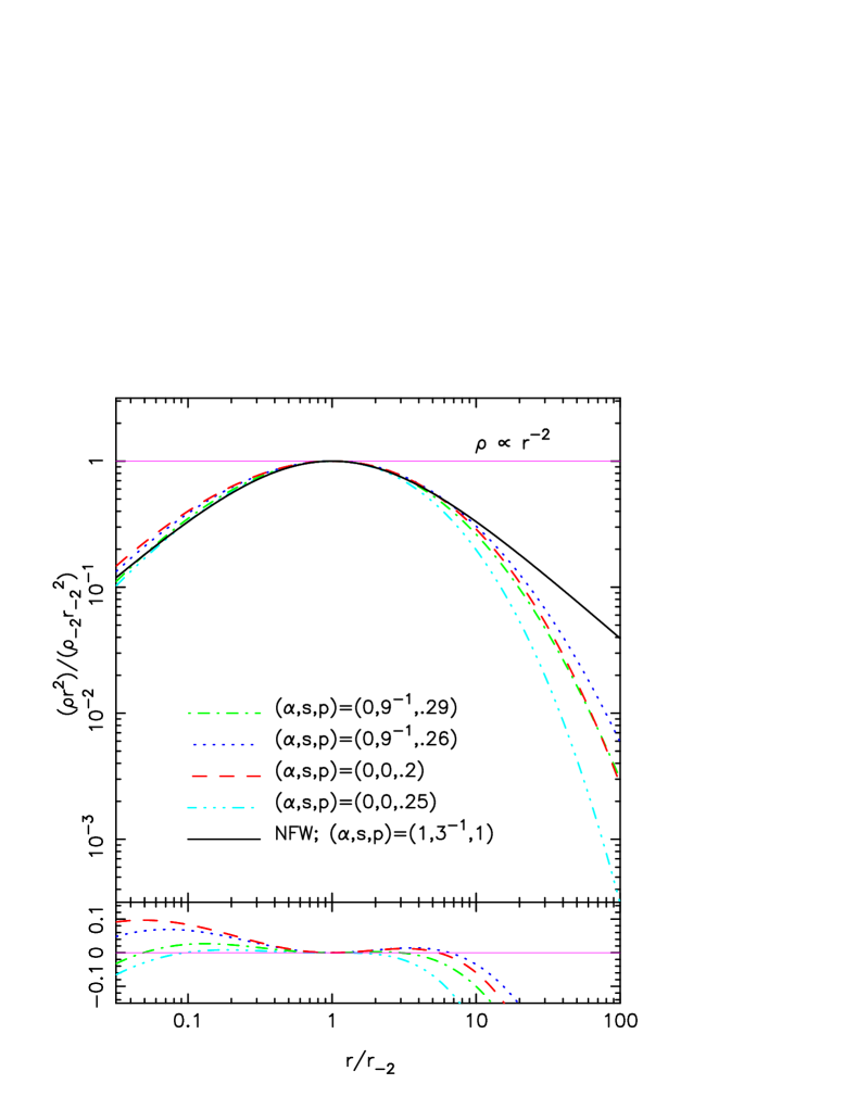
In Figure 5, we plot the density profiles of some cored double power-law models and the Einasto profile compared to the NFW profile and the Hernquist model. The models are deliberately chosen so that they closely approximate the latter models near $r\approx r_{-2}$ except that they are constrained to possess a core rather than a cusp at the centre. The finite resolution prevents any information on the density profile near the very centre from being available to us. For any practical fitting, thus there essentially exists an inner cut-off radius below which the behaviour of the density profile is immaterial. Furthermore, no dark halo is in isolation in reality and so the power index for the asymptotic fall-off is an idealized construct. In fact, the fitting to the density profile should be cut off before the local halo density approaches the non-zero background value. However, there is no obvious theoretical prejudice regarding the location of this truncation radius relative to the transition zone of the double power-law profile. That is to say, the outer logarithmic slopes of simulated dark haloes simply correspond to that at the truncation radius, rather than the ‘true’ asymptotic slope, and there is no obvious argument for the former to be close to the latter. With external factors such as tidal effects and hierarchical environments affecting the outer cut-off, it is thus possible for the halo to have the local logarithmic slope of $\approx 3$ at truncation as reported by many simulations whilst the ‘true’ asymptotic slope, if extrapolated, would be steeper (even exponential). These observations and the uncertainties in the fitting suggest that, given the fitting is weighted near $r_{-2}$, the distinction between the conventional double power law and a cored profile with a sufficiently broad transition zone afforded by small $p$ is nontrivial and they may even be degenerate in some degree.

In practice, the presence of the central density cores versus cusps in dark haloes may be discriminated by observing $\gammaup$-ray signals at the Galactic centre due to pair annihilations of CDM particles (but see also Zhao & Silk, 2005). In the following (Sect. 4.3), we shall briefly analyze the behaviour of the so-called astrophysical term $J(\phi)$ (e.g., Lapi et al., 2010) in the CDM annihilation signal for the dark halo density profile given by our model family. We find that if the dark halo density profile diverges faster than $r^{-1/2}$ as $r\rightarrow 0$, the astrophysical term also formally diverges as $\phi\rightarrow 0$ – in particular, the $r^{-\alpha}$ cusp ($\alpha>\frac{1}{2}$) results in $J\in\varTheta(\phi^{-(2\alpha-1)})$. Whilst the finite angular resolution indicates that the observed signal should be finite (unless the density cusp is steeper than $r^{-3/2}$), the signal from the $r^{-1}$ cusp of an NFW halo should be significantly stronger than that from a cored halo provided that both are normalized locally in the Solar neighbourhood. For example, Lapi et al. (2010) find that the NFW halo produces one to two orders of magnitude stronger annihilation signal towards the Galactic centre than the Einasto model with the resolution ranging from $\approx 3~{}\mbox{deg}^{2}$ to $\approx 100~{}\mbox{arcmin}^{2}$.

4.2 Surface density profiles

In terms of the comparison to the real astronomical observations, it is important to fold the effect of projection into our models. The most basic among these is the integrated mass density along the line of sight (i.e., the surface density profile) given by

$$\Sigma(R)=2\int_{R}^{\infty}\frac{\varrho(r)\,r\,\mathrm{d}r}{\sqrt{r^{2}-R^{2}}}.$$ (7)

This is of use for the lensing convergence $\kappa(R)$ of a halo or the surface brightness profile $I(R)$ of a ‘transparent’ constant mass-to-light ratio stellar spheroid, both of which are proportional to $\Sigma(R)$. If $s\geq 1$ ($0\leq\delta\leq 1$), then equation (7) diverges for any finite $R$ and so $\Sigma(R)$ is not well defined. For the remaining cases that $0\leq s<1$ ($\delta>1$), the result can in principle be evaluated numerically – for an arbitrary parameter combination, the integral in general results in the Fox H-function, but the particular results are in practice rather ‘useless’ for the purpose of calculations.

With the cusp/core problem in mind, the important characteristics of the surface density profiles of note are their limiting behaviours. The leading terms of $\Sigma(R)$ as $R\rightarrow 0$ or $R\rightarrow\infty$ may be obtained by analyzing equation (7) without actually resolving the integral. The fundamental results in these regards are

$$\frac{\Sigma(0)}{\bar{\varrho}_{\mathrm{s}}r_{\mathrm{s}}}=\frac{2}{p}\,\Gamma\left(\frac{1-\alpha}{p}\right)\times\begin{cases}\dfrac{\delta^{(1-\alpha)/p}\Gamma\bigl{(}\frac{\delta-1}{p}\bigr{)}}{\Gamma\bigl{(}\frac{\delta-\alpha}{p}\bigr{)}}&(s>0)\\ p^{(1-\alpha)/p}&(s=0)\end{cases},$$ (8a)

$$\lim_{R\rightarrow 0}\frac{\Sigma(R)}{R\,\varrho(R)}=\mathrm{B}\!\left(\frac{1}{2},\frac{\alpha-1}{2}\right)\,;\quad\lim_{R\rightarrow\infty}\frac{\Sigma(R)}{R\,\varrho(R)}=\mathrm{B}\!\left(\frac{1}{2},\frac{\delta-1}{2}\right),$$ (8b)

where $\Gamma(u)$ and $\mathrm{B}(u,w)$ are the gamma and beta functions. Equation (8a) is valid for $\alpha<1$ whereas equations (8a) are finite for $\alpha>1$ and $\delta>1$, respectively. That is to say, the surface density at $R=0$ is finite for $0\leq\alpha<1$ whilst it is cusped as $R^{-(\alpha-1)}\rightarrow\infty$ near $R=0$ if $\alpha>1$ and it falls off like $R^{-(\delta-1)}$ for $s>0$ ($\delta>0$). Please see Appendix C (also An & Evans, 2009, sect. 6) for more details.

4.3 The Emission measure

From the mathematical point of view, the quantity defined such that

$$\mathcal{J}\equiv\int_{\rm l.o.s.}\!\varrho^{2}\mathrm{d}\ell=2\int_{R}^{\infty}\frac{[\varrho(r)]^{2}r\,\mathrm{d}r}{\sqrt{r^{2}-R^{2}}}$$ (9)

shares common properties with the surface density defined in equation (7), corresponding to the parameter set of $(2\alpha,2\delta)$. This is related to the emission measure of the free-free radiation (Bremsstrahlung) and the so-called astrophysical term in the CDM annihilation signal from an external dark halo. For the dark halo of the Milky Way, the astrophysical term defined to be

$$J(\phi)=\begin{cases}{\displaystyle\int_{r_{\phi}}^{r_{\mathrm{v}}}\!\frac{[\varrho(r)]^{2}r\,\mathrm{d}r}{(r^{2}-r_{\phi}^{2})^{1/2}}+\int_{r_{\phi}}^{r_{\odot}}\!\frac{[\varrho(r)]^{2}r\,\mathrm{d}r}{(r^{2}-r_{\phi}^{2})^{1/2}}}&(0\leq\phi\leq\frac{\pi}{2})\\ {\displaystyle\int_{r_{\odot}}^{r_{\mathrm{v}}}\!\frac{[\varrho(r)]^{2}r\,\mathrm{d}r}{(r^{2}-r_{\phi}^{2})^{1/2}}}&(\frac{\pi}{2}\leq\phi\leq\pi)\end{cases};$$ (10)

with $r_{\phi}=r_{\odot}\sin\phi$ is more relevant to the actual observable signal. Here $r_{\mathrm{v}}$ is the virial radius of the Galactic dark halo, $r_{\odot}$ is the Galactocentric distance of the Sun and $\phi$ is the angle between the line of sight and the Galactic centre.

Analogous to $\Sigma(R)$, the general analytical expressions of $\mathcal{J}(R)$ or $J(\phi)$ for the three-dimensional density profiles considered in this paper are expressible using the Fox H-function whilst their numerical evaluations may be achieved straightforwardly through the quadrature sum. The limiting behaviours of $\mathcal{J}$ as $R\rightarrow 0$ are found similarly. In particular, for a cusped profile $\varrho\in\varTheta(r^{-\alpha})$ with $\alpha>0$,

$$\mathcal{J}\in\begin{cases}\varTheta(R^{-(2\alpha-1)})&(\alpha>\frac{1}{2})\\ \varTheta(\ln R^{-1})&(\alpha=\frac{1}{2})\\ \varTheta(1)&(\alpha<\frac{1}{2})\end{cases}$$ (11a)

$$\left\lvert{\mathcal{J}(0)-\mathcal{J}(R)}\right\rvert\sim A^{\prime}R^{1-2\alpha}\quad(0<\alpha<\tfrac{1}{2}),$$

whilst we find $$\mathcal{J}\in\varTheta(1)$$ and

$$\left\lvert{\mathcal{J}(0)-\mathcal{J}(R)}\right\rvert\in\begin{cases}\varTheta(R^{1+p})&(0<p<1)\\ \varTheta(R^{2}\ln R^{-1})&(p=1)\\ \varTheta(R^{2})&(p>1)\end{cases}$$ (11b)

for a cored profile such that $\left\lvert{\varrho(0)-\varrho(r)}\right\rvert\sim Ar^{p}$. As for $J(\phi)$, we note $J(\phi)\sim\mathcal{J}(r_{\odot}\sin\phi)$ and $\sin\phi\sim\phi$ as $\phi\rightarrow 0$. It then follows that $J(\phi)$ diverges as $\phi^{-(2\alpha-1)}$ or $\ln\phi^{-1}$ for a cusped halo with $\alpha>\frac{1}{2}$ or $\alpha=\frac{1}{2}$. On the other hand, $J(\phi=0)$ should be finite if the Galactic CDM halo is cored or cusped slower than $r^{-1/2}$. These last cases may in principle be discriminated by examining $\mathrm{d}J/\mathrm{d}\phi$, which formally diverges for a cusped halo as $\phi\rightarrow 0$ whilst it vanishes for a cored halo at the same limit. We leave more detailed studies of the projected properties of the models for the future.

Appendix A Elementary Integral Properties

A.1 The Enclosed mass

The mass enclosed in a sphere of radius $r$ is obtained by

$$M_{r}=4\pi\int_{0}^{r}\!\varrho(u)\,u^{2}\mathrm{d}u.$$ (12a)

With our models, we should limit $$\alpha<3 r^{2-\alpha} r\rightarrow 0$$ since the integrand behaves like as (if otherwise, this diverges). This is directly related to the gravitational acceleration and the circular speed,

$$\left\lVert\mn@boldsymbol{g}\right\rVert=\frac{\varv_{\mathrm{c}}^{2}}{r}=\frac{GM_{r}}{r^{2}}.$$ (12b)

For $\alpha<3$, $p>0$, and $s=\delta^{-1}>0$, equation (12a) results in

$$M_{r}=\frac{4\pi C_{M}}{p}\,B\left(\frac{x^{p}}{1+x^{p}};\frac{3-\alpha}{p},\frac{\delta-3}{p}\right),$$ (13a)

$$C_{M}=\frac{\bar{\varrho}_{\mathrm{s}}r_{\mathrm{s}}^{3}}{s^{(3-\alpha)/p}}=\varrho_{-2}\,r_{-2}^{3}\left[\frac{(\delta-\alpha)^{\delta-\alpha}}{(2-\alpha)^{3-\alpha}(\delta-2)^{\delta-3}}\right]^{1/p}.$$

where

$$x^{p}=\frac{r^{p}}{a^{p}}=\frac{r^{p}}{\delta\,r_{\mathrm{s}}^{p}}=s\,\frac{r^{p}}{r_{\mathrm{s}}^{p}}=\frac{2-\alpha}{\delta-2}\left(\frac{r}{r_{-2}}\right)^{p},$$ (13b)

whilst $B(z;u,w)\equiv\mathrm{B}_{z}(u,w)$ is the incomplete beta function. The beta function is efficiently evaluated using series or continued fractions, which converge typically faster than integrating equation (12a) via the quadrature sum. Some reduce to expressions involving only elementary (algebraic and logarithmic or inverse trigonometric/hyperbolic) functions, which are in general possible if any of the following is true:

• $(3-\alpha)/p$ or $(\delta-3)/p$ is a positive integer,

• $(\delta-\alpha)/p$ is a zero or a negative integer,

• $(\delta-3)/p$ is an integer and $(3-\alpha)/p$ is a positive rational, or

• both $2(3-\alpha)/p$ and $2(\delta-3)/p$ are integers.

Equation (12a) for $s=0$ on the other hand results in

$$M_{r}=\frac{4\pi C_{M,0}}{p}\,\gamma\left(\frac{3-\alpha}{p};y^{p}\right),$$ (14a)

$$C_{M,0}=\bar{\varrho}_{\mathrm{s}}r_{\mathrm{s}}^{3}p^{(3-\alpha)/p}=\varrho_{-2}\,r_{-2}^{3}\mathrm{e}^{(2-\alpha)/p}\left(\frac{p}{2-\alpha}\right)^{(3-\alpha)/p}.$$

where $$\alpha<3 p>0$$, and

$$y^{p}=\frac{r^{p}}{pr_{\mathrm{s}}^{p}}=\frac{2-\alpha}{p}\left(\frac{r}{r_{-2}}\right)^{p}.$$ (14b)

Here, $\gamma(u;z)$ is the lower incomplete gamma function. This ‘simplifies’ to elementary (up to exponential) functions if $(3-\alpha)/p$ is a positive integer. It is also recast to formulae using the error function and elementary functions for half-integer values of $(3-\alpha)/p$.

The behaviour of the integrand, $r^{2-\delta}$ as $r\rightarrow\infty$ of equation (12a) indicates that the finite total mass is defined for $\delta>3$ (including the $s=0$ case). In particular,

$$M_{\mathrm{tot}}=\begin{cases}{\displaystyle\frac{4\pi C_{M}}{p}\,\mathrm{B}\!\left(\frac{3-\alpha}{p},\frac{\delta-3}{p}\right)}&(0<s<\tfrac{1}{3})\vskip 3.0pt plus 1.0pt minus 1.0pt\\ {\displaystyle\frac{4\pi C_{M,0}}{p}\,\Gamma\!\left(\frac{3-\alpha}{p}\right)}&(s=0)\end{cases}$$ (15)

where $\mathrm{B}(u,w)=B(1;u,w)=\Gamma(u)\Gamma(w)/\Gamma(u+w)$ is the beta function and $\Gamma(u)=\gamma(u;\infty)$ is the gamma function. If $s\geq\frac{1}{3}$ ($\delta\leq 3$) on the other hand, then the total mass is infinite. Specifically, the enclosed mass diverges logarithmically if $\delta=3$ or like $r^{3-\delta}$ if $\delta<3$.

A.2 The Gravitational potential

The potential of an isolated system up to an additive constant is found by integrating $\mn@boldsymbol{\nabla}\psi=-\mn@boldsymbol{g}$. Under spherical symmetry,

$$\frac{\mathrm{d}\psi}{\mathrm{d}r}=\frac{GM_{r}}{r^{2}}=-\frac{\mathrm{d}}{\mathrm{d}r}\left(\frac{GM_{r}}{r}\right)+4\pi G\varrho r$$ (16)

where we have used $\mathrm{d}M_{r}/\mathrm{d}r=4\pi\varrho r^{2}$. Then the potential behaves asymptotically like $r^{-1}$, $r^{-1}\ln r$, $r^{-(\delta-2)}$ and $\ln r$ for $\delta>3$, $\delta=3$, $\delta<3$ but $\delta\neq 2$, and $\delta=2$, respectively. If $\delta>2$, the potential at infinity is not divergent and any particle with enough kinetic energy can escape to an unbound state. By contrast, if $\delta\leq 2$, then $\psi\rightarrow\infty$ as $r\rightarrow\infty$, and thus every tracer particle in the model with $s\geq\frac{1}{2}$ is bound to the system and escape is formally impossible.

If $0\leq s<\frac{1}{2}$ ($\delta>2$), it is customary to set $\psi(\infty)=0$ and thus

$$\psi(r)-\cancel{\psi_{\infty}}=-\frac{GM_{r}}{r}-4\pi G\int_{r}^{\infty}\!\varrho(u)\,u\,\mathrm{d}u.$$ (17)

For $s=\delta^{-1}>0$,

$$\frac{\psi}{4\pi G}=-\frac{C_{\psi}}{p}\left[\frac{1}{x}\,B\left(\frac{x^{p}}{1+x^{p}};\frac{\tilde{\alpha}_{3}}{p},\frac{\hat{\delta}_{3}}{p}\right)+B\left(\frac{1}{1+x^{p}};\frac{\hat{\delta}_{2}}{p},\frac{\tilde{\alpha}_{2}}{p}\right)\right],$$ (18)

$$C_{\psi}=\frac{C_{M}}{\delta^{1/p}r_{\mathrm{s}}}=\bar{\varrho}_{\mathrm{s}}r_{\mathrm{s}}^{2}\delta^{\tilde{\alpha}_{2}/p}=\varrho_{-2}\,r_{-2}^{2}\left[\frac{(\delta-\alpha)^{\delta-\alpha}}{{\tilde{\alpha}_{2}}^{\tilde{\alpha}_{2}}{\hat{\delta}_{2}}^{\hat{\delta}_{2}}}\right]^{1/p},$$

whilst, for $s=0$,

$$\frac{\psi}{4\pi G}=-\frac{C_{\psi,0}}{p}\left[\frac{1}{y}\,\gamma\left(\frac{\tilde{\alpha}_{3}}{p};y^{p}\right)+\varGamma\left(\frac{\tilde{\alpha}_{2}}{p};y^{p}\right)\right],$$ (19)

$$C_{\psi,0}=\frac{C_{M,0}}{p^{1/p}r_{\mathrm{s}}}=\bar{\varrho}_{\mathrm{s}}r_{\mathrm{s}}^{2}p^{\tilde{\alpha}_{2}/p}=\varrho_{-2}\,r_{-2}^{2}\left(\frac{\mathrm{e}}{\tilde{\alpha}_{2}/p}\right)^{\tilde{\alpha}_{2}/p}.$$

where $\varGamma(u;z)$ is the upper incomplete gamma function. We also use short-hand notation, $\tilde{\alpha}_{n}=(n-\alpha)$ and $\hat{\delta}_{n}=(\delta-n)$ for an integer $n$. These again reduce to expressions involving only elementary functions if $M_{r}$ is expressible in such a way and the parameter combinations $\hat{\delta}_{2}/p$ and $\tilde{\alpha}_{2}/p$ satisfy criteria similar to those applied for $\hat{\delta}_{3}/p$ and $\tilde{\alpha}_{3}/p$. Some specific examples are found in Appendix D.

The integral in equation (17) for $\delta\leq 2$ is divergent, and so equation (18) for such are meaningless (although they are technically well-defined unless $\hat{\delta}_{2}/p$ is a negative integer). The potential for $\delta\leq 2$ however can still be defined with an alternative zeropoint. Since $M_{r}\in\varTheta(r^{3-\alpha})$ as $r\rightarrow 0$, we have $\psi\in\varTheta(r^{2-\alpha})$ if $\alpha\neq 2$ or $\varTheta(\ln r^{-1})$ for $\alpha=2$ in the same limit. Hence, provided that $\alpha<2$ (note that we have generally restricted to be $\alpha<\delta$), the alternative reference for the potential $\psi(0)=0$ is well-defined and

$$\psi(r)-\cancel{\psi_{0}}=-\frac{GM_{r}}{r}+4\pi G\int_{0}^{r}\!\varrho(u)\,u\,\mathrm{d}u.$$ (20)

For $s>0$, this results in

$$\frac{\psi}{4\pi G}=\frac{C_{\psi}}{p}\left[B\left(\frac{x^{p}}{1+x^{p}};\frac{\tilde{\alpha}_{2}}{p},\frac{\hat{\delta}_{2}}{p}\right)-\frac{1}{x}\,B\left(\frac{x^{p}}{1+x^{p}};\frac{\tilde{\alpha}_{3}}{p},\frac{\hat{\delta}_{3}}{p}\right)\right]$$ (21)

If $\alpha<2<\delta$, both this and equation (18) are well-defined, but they differ by a constant (independent of $r$) – note $B(1-z;u,w)+B(z;w,u)=\mathrm{B}(u,w)$ for $u,w>0$. This difference corresponds to the depth of the central potential well, $\left\lvert{\psi_{\infty}-\psi_{0}}\right\rvert$. This and $\sqrt{2\left\lvert{\psi_{\infty}-\psi_{0}}\right\rvert}$ are also the maximum specific energy and speed of any bound particle in the system.

For $s=0$, equation (19) is always (provided that $\alpha<3$) well-defined. That is to say, since the total mass is finite, it is always possible to set $\psi(\infty)=0$. The central potential well depth is then the limit of equation (19) as $r\rightarrow 0$, which is finite if $\alpha<2$. Using this and $\gamma(u;z)+\varGamma(u;z)=\Gamma(u)$ for $u>0$, it is possible to derive an alternative expression for equation (19) for $\alpha<2$, that is

$$\frac{\psi_{0}-\psi}{4\pi G}=\frac{C_{\psi,0}}{p}\left[\frac{1}{y}\,\gamma\left(\frac{\tilde{\alpha}_{3}}{p};y^{p}\right)-\gamma\left(\frac{\tilde{\alpha}_{2}}{p};y^{p}\right)\right]$$ (22)

of which the zero point reference is essentially at the centre.

Appendix B Tractable Dynamical Properties

B.1 Velocity dispersions

The velocity dispersion profile of a spherical system is found by integrating the spherical steady-state Jeans equation,

$$\frac{1}{\varrho}\frac{\mathrm{d}(\varrho\sigma_{r}^{2})}{\mathrm{d}r}+\frac{2\sigma_{r}^{2}-(\sigma_{\theta}^{2}+\sigma_{\phi}^{2})}{r}+\frac{GM_{r}}{r^{2}}=0.$$ (23)

Equation (23) may be integrated to be

$$\sigma_{r}^{2}(r)=\frac{1}{\varrho(r)}\!\int_{r}^{\infty}\!\mathrm{d}s\frac{GM_{s}}{s^{2}}\varrho(s)\exp\!\left\lgroup\int_{r}^{s}\!\mathrm{d}u\frac{2\beta(u)}{u}\right\rgroup$$ (24)

given the boundary condition $\lim_{r\rightarrow\infty}\varrho\sigma_{r}^{2}=0$, once $\varrho(r)$ and $M_{r}$, as well as the so-called velocity anisotropy parameter

$$\beta(r)\equiv 1-\frac{\sigma_{\theta}^{2}+\sigma_{\phi}^{2}}{2\sigma_{r}^{2}}.$$ (25)

are specified. For a monotonically-varying anisotropy parameter, the parametrization introduced by Baes & Van Hese (2007),

$$\beta=\frac{\beta_{\infty}r^{2q}+\beta_{0}r_{\mathrm{a}}^{2q}}{r^{2q}+r_{\mathrm{a}}^{2q}}=\frac{\mathrm{d}\log\bigl{[}r^{2\beta_{0}}(r^{2q}+r_{\mathrm{a}}^{2q})^{(\beta_{\infty}-\beta_{0})/q}\bigr{]}}{\mathrm{d}\log r^{2}}$$ (26)

may be useful to represent its behaviour. Then, equation (24) results in a simple integral quadrature for $\sigma_{r}^{2}(r)$, namely,

$$\sigma_{r}^{2}(r)=\frac{1}{h(r)}\!\int_{r}^{\infty}\!\frac{GM_{u}}{u^{2}}\,h(u)\,\mathrm{d}u;$$ (27a)

$$h(r)=r^{2\beta_{0}}(r^{2q}+r_{\mathrm{a}}^{2q})^{(\beta_{\infty}-\beta_{0})/q}\varrho(r).$$ (27b)

which can be evaluated numerically if $M_{r}$ is tabulated. Since $h\in\varTheta(r^{2\beta_{\infty}-\delta})$ as $r\rightarrow\infty$, this is convergent provided that $1+\beta_{\infty}<\delta$ (cf., Hansen, 2004, see also An & Evans 2006). Given $\beta\leq 1$, equation (27a) is therefore well defined for $\delta>2$.

An & Evans (2006, 2009) have analyzed the leading term behaviours of $\sigma_{r}^{2}$ in the limit of $r\rightarrow 0$ and $r\rightarrow\infty$. The complete analytic expressions for arbitrary parameter combinations are yet possible only with higher transcendental functions, which are more or less impractical. For some parameter combinations however, reductions to simpler functions are available. If $\beta$ is a linear function of the logarithmic density slope (Hansen & Moore, 2006), then $r_{\mathrm{a}}=a$ and $2q=p$, and so $h(r)$ in equation (27b) also takes the form of a double power law for $s>0$. If $M_{r}$ is additionally reducible to the sum of such factors (e.g., $\hat{\delta}_{3}/p$ or $\tilde{\alpha}_{3}/p$ is a positive integer), then $\sigma_{r}^{2}$ is expressible using the sum of incomplete beta functions. The simplest example is the $\delta=p+3$ case, for which

$$\sigma_{r}^{2}=\frac{4\pi GC_{\psi}}{p\tilde{\alpha}_{3}}x^{\alpha-2\beta_{0}}(1+x^{p})^{1-\frac{2(\beta_{\infty}-\beta_{0})-\tilde{\alpha}_{3}}{p}}\\ \times B\left(\frac{1}{1+x^{p}};\frac{2(2-\beta_{\infty})}{p}+1,\frac{2(1+\beta_{0}-\alpha)}{p}\right).$$ (28)

This includes the $\gamma$-sphere for which $p=1$ and $\delta=4$, the model studied by Evans & An (2005) for which $(\alpha,\delta)=(2-p,p+3)$, and the analytical solutions of Dehnen & McLaughlin (2005) for which $(\alpha,\delta)=(1+\beta_{0}-\frac{p}{2},p+3)$. Note $B(z;u,1)=z^{u}/u$, and so $\sigma_{r}^{2}$ for this last case results in a double power law as the density profile. The resulting model with $p=2(2-\beta_{0})(\varepsilon-2)/(\varepsilon+6)$ exhibits radial power-law behaviour, $\varrho/\sigma_{r}^{\varepsilon}\propto r^{-\eta}$ where $\eta=\alpha\varepsilon/2+\alpha-\beta_{0}\varepsilon$ as noted by Dehnen & McLaughlin (2005). Equation (28) also indicates that $\sigma_{r}^{2}\sim\sigma^{2}/(3-2\beta_{\infty})\sim\varv_{\mathrm{c}}^{2}/(p+4-2\beta_{\infty})$ as $r\rightarrow\infty$ whereas, as $r\rightarrow 0$, we find that $\sigma_{r}^{2}\in\varTheta(r^{\alpha-2\beta_{0}})$, $\varTheta(r^{2-\alpha}\ln r^{-1})$, and $\varTheta(r^{2-\alpha})$ for $1+\beta_{0}>\alpha$, $1+\beta_{0}=\alpha$, and $1+\beta_{0}<\alpha$ respectively. These are consistent with behaviours deduced by An & Evans (2006).

B.2 Constant-anisotropy distribution functions

Consider the phase-space distribution given by

$$\mathcal{F}(\mathcal{E},L^{2})=\begin{cases}\dfrac{2^{\beta-\frac{3}{2}}g(\mathcal{E})}{\pi^{3/2}\Gamma(1-\beta)\,L^{2\beta}}&(\beta<1)\vskip 3.0pt plus 1.0pt minus 1.0pt\\ \dfrac{\deltaup(L^{2})\,g(\mathcal{E})}{\sqrt{2}\pi^{3/2}}&(\beta=1)\end{cases}$$ (29)

where $\mathcal{E}$ and $L$ are the specific binding energy and the magnitude of the specific angular momentum and $\deltaup(w)$ is the Dirac delta. This builds a spherical system with the anisotropy parameter at all radii given by the parameter value $\beta$. The function $g(\mathcal{E})$ is related to the tracer energy distribution via

$$\frac{\mathrm{d}\varrho}{\mathrm{d}\mathcal{E}}=\frac{\left\lvert{\Psi-\mathcal{E}}\right\rvert^{\frac{1}{2}-\beta}\Theta(\Psi-\mathcal{E})}{\Gamma\bigl{(}\frac{3}{2}-\beta\bigr{)}\,r^{2\beta}}\,g(\mathcal{E})$$ (30)

$$\frac{\mathrm{d}M}{\mathrm{d}\mathcal{E}}=\frac{N(\mathcal{E})\,g(\mathcal{E})}{\Gamma\bigl{(}\frac{3}{2}-\beta\bigr{)}}\,;\quad N(\mathcal{E})=4\pi\!\int_{0}^{r_{\mathcal{E}}}\,\left\lvert{\Psi-\mathcal{E}}\right\rvert^{\frac{1}{2}-\beta}r^{2(1-\beta)}\mathrm{d}r,$$

where $\Theta(w)$ is the Heaviside unit step function and $r_{\mathcal{E}}$ is the farthest distance to which a particle with the binding energy $\mathcal{E}$ can move, that is, $\Psi(r_{\mathcal{E}})=\mathcal{E}$. Here, $\mathrm{d}\varrho/\mathrm{d}\mathcal{E}$ and $\mathrm{d}M/\mathrm{d}\mathcal{E}$ are the local and global differential energy distributions and $N(\mathcal{E})$ is the marginalized density of states. The function $\Psi(r)$ defined to be

$$\Psi(r)\equiv\begin{cases}\psi(r_{\mathrm{out}})-\psi(r)&\text{if $r_{\mathrm{out}}$ is finite}\\ \psi(\infty)-\psi(r)&\text{if $r_{\mathrm{out}}=\infty$ and $\left\lvert{\psi(\infty)}\right\rvert<\infty$}\\ -\psi(r)&\text{if $r_{\mathrm{out}}=\infty$ and $\psi(\infty)\rightarrow\infty$}\\ \end{cases}$$ (31a)

is the positive potential function where $$r_{\mathrm{out}} \mathcal{E}=\Psi-\frac{1}{2}\varv^{2} \varv$$ is the boundary radius. The specific binding energy is given by where is the speed of the tracer with its lower bound for bound particles being

$$\underline{\mathcal{E}}\equiv\begin{cases}0&\text{for an escapable system}\\ -\infty&\text{for an infinitely-extended inescapable system}\end{cases}.$$ (31b)

The undetermined function $g(\mathcal{E})$ is uniquely specified by the density profile. That is, integrating equation (29) over the accessible velocity space at a fixed location results in the augmented density $h(\Psi)=r^{2\beta}\varrho$ as a function of $\Psi$. The function $g(\mathcal{E})$ then may be determined by its inversion, the Eddington–Cuddeford formula,

$$g(\mathcal{E})=\frac{1}{\Gamma(1-\epsilon)}\frac{\mathrm{d}}{\mathrm{d}\mathcal{E}}\!\int_{\underline{\mathcal{E}}}^{\mathcal{E}}\!\frac{h^{(\mu)}(\Psi)\,\mathrm{d}\Psi}{(\mathcal{E}-\Psi)^{\epsilon}}\\ =\begin{cases}{\displaystyle\frac{1}{\Gamma(1-\epsilon)}\left[\int_{\underline{\mathcal{E}}}^{\mathcal{E}}\!\!\frac{h^{(\mu+1)}(\Psi)\,\mathrm{d}\Psi}{(\mathcal{E}-\Psi)^{\epsilon}}+\frac{h^{(\mu)}(\underline{\mathcal{E}})}{(\mathcal{E}-\underline{\mathcal{E}})^{\epsilon}}\right]}&(0<\epsilon<1)\\ \ h^{(\mu)}(\mathcal{E})&(\epsilon=0)\end{cases}$$ (32)

where $\mu=\lfloor\frac{3}{2}-\beta\rfloor$ and $\epsilon=(\frac{3}{2}-\beta)-\mu$ are the integer floor and the fractional part of $\frac{3}{2}-\beta$. Equation (32) indicates that, given the inverse function $r(\psi)=\psi^{-1}(\psi)$ of $\psi=\psi(r)$ and the augmented density $h(\Psi)=[r({-\Psi})]^{2\beta}\varrho[r({-\Psi})]$, the distribution function (df) of the form of equation (29) is available as an integral quadrature. If $\beta$ is a half-integer (i.e., $\beta=\frac{1}{2},-\frac{1}{2},\dotsc$), the formula results in pure differentiation (Cuddeford, 1991; Evans & An, 2006).

B.2.1 the $(\alpha,\delta)=(2-p,3+p)$ case

The simplest example is the $(\alpha,\delta)=(2-p,3+p)$ case, for which

$$h(\Psi)=\frac{\bar{\varrho}a^{2\beta}\Phi^{p+3-2\beta}}{(1-\Phi^{p})^{2(1-\beta)/p-1}}\,;\quad\Phi=\frac{\Psi}{\left\lvert{\psi_{\infty}-\psi_{0}}\right\rvert}=\frac{(p+1)\Psi}{4\pi G\bar{\varrho}a^{2}}.$$ (33a)

Here, $$\left\lvert{\psi_{\infty}-\psi_{0}}\right\rvert=GM_{\mathrm{tot}}/a=4\pi G\bar{\varrho}a^{2}/(1+p) 0\leq\Phi\leq 1$$ is the depth of the central potential (note ). The df is then found with

$$\begin{split}g(\mathcal{E})&=\frac{\bar{\varrho}a^{2\beta}}{\left\lvert{\psi_{\infty}-\psi_{0}}\right\rvert^{3/2-\beta}}\tilde{\varg}\left(\frac{\mathcal{E}}{\left\lvert{\psi_{\infty}-\psi_{0}}\right\rvert}\right),\\ \tilde{\varg}(\Phi)&=\frac{1}{\Gamma(1-\epsilon)}\!\int_{0}^{\Phi}\!\!\frac{\mathrm{d}Q}{(\Phi-Q)^{\epsilon}}\frac{\mathrm{d}^{\mu+1}}{\mathrm{d}Q^{\mu+1}}\!\left[\frac{Q^{p+3-2\beta}}{(1-Q^{p})^{2(1-\beta)/p-1}}\right].\end{split}$$ (33b)

If $2(1-\beta)\geq p>0$, the df is non-negative for all accessible binding energy interval, $0\leq\mathcal{E}\leq\left\lvert{\psi_{\infty}-\psi_{0}}\right\rvert$ (cf., An & Evans, 2006). Equation (33b) with arbitrary $p>0$ and $\beta<1$ results in the Fox H-function, which is equivalent a power series of $\Phi$, namely,

$$\tilde{\varg}(\Phi)=\Phi^{p+\frac{3}{2}-\beta}\sum_{k=0}^{\infty}\frac{(\beta_{p})_{k}\Gamma(pk+p+4-2\beta)}{k!\Gamma\bigl{(}pk+p+\frac{5}{2}-\beta\bigr{)}}\,\Phi^{pk},$$ (34)

where $\beta_{p}=2(1-\beta)/p-1>0$ and $(a)_{k}$ is the Pochhammer symbol. This reduces to a hypergeometric function if $p$ is rational. The result for the Hernquist model was derived by Baes & Dejonghe (2002),

$$\tilde{\varg}(\Phi)=\frac{\Gamma(5-2\beta)}{\Gamma\bigl{(}\frac{7}{2}-\beta\bigr{)}}\,\Phi^{\frac{5}{2}-\beta}{}_{2}F_{1}\Bigl{(}1-2\beta,5-2\beta;\tfrac{7}{2}-\beta;\Phi\Bigr{)},$$ (35)

whilst for the Schuster-Plummer sphere, this becomes

$$\tilde{\varg}(\Phi)=\frac{\Gamma(6-2\beta)}{\Gamma(\frac{9}{2}-\beta)}\,\Phi^{\frac{7}{2}-\beta}{}_{3}F_{2}\Bigl{(}-\beta,3-\beta,\tfrac{7}{2}-\beta;\tfrac{9-2\beta}{4},\tfrac{11-2\beta}{4};\Phi^{2}\Bigr{)}.$$ (36)

If $\beta$ is a half-integer, both are expressible using only algebraic functions whereas equation (35) with an integer $\beta$ reduces to an expression involving up to inverse trigonometric functions, e.g., for the isotropic Hernquist model,

$$\tilde{\varg}(\Phi)=\frac{1}{2\!\!\sqrt{\pi}}\left[\frac{3\arcsin\!\!\sqrt{\Phi}}{(1-\Phi)^{\frac{5}{2}}}-\frac{\!\!\sqrt{\Phi}\,(1-2\Phi)(3+8\Phi-8\Phi^{2})}{(1-\Phi)^{2}}\right].$$ (37)

If $2(1-\beta)=p$, equation (33b) indicates that $\tilde{\varg}(\Phi)\propto\Phi^{p+\frac{3}{2}-\beta}=\Phi^{(3p+1)/2}$. Equation (34) is still valid because the series then terminates for $k\geq 1$. The corresponding df, $\mathcal{F}(\mathcal{E},L^{2})\propto L^{p-2}\mathcal{E}^{(3p+1)/2}$ is the hypervirial model studied by Evans & An (2005).

B.2.2 the distribution function as a function of $r_{\mathcal{E}}$

Even if an analytic expression for the inverse function of the potential is not available, equation (32) can be used to write down $g(\mathcal{E})$ implicitly using $r_{\mathcal{E}}=\Psi^{-1}(\mathcal{E})=\psi^{-1}({-\mathcal{E}})$. This is achieved through change of variables for the integral in equation (32),

$$\begin{split}g(\mathcal{E})&=\frac{1}{\Gamma(1-\epsilon)}\frac{\mathrm{d}^{\mu+1}}{\mathrm{d}\mathcal{E}^{\mu+1}}\!\int_{r_{\mathcal{E}}}^{\infty}\frac{GM_{r}\,\varrho(r)\,\mathrm{d}r}{r^{2(1-\beta)}[\mathcal{E}-\Psi(r)]^{\epsilon}}\\ &=\frac{(-1)^{\mu}}{\Gamma(1-\epsilon)}\frac{r_{\mathcal{E}}^{2}}{M_{r_{\mathcal{E}}}}\frac{\mathrm{d}}{\mathrm{d}r_{\mathcal{E}}}\!\int_{\infty}^{r_{\mathcal{E}}}\frac{M_{r}\,\hat{\varg}_{2\beta}^{\mu}(r)\,\mathrm{d}r}{r^{2}[\mathcal{E}-\Psi(r)]^{\epsilon}}\end{split};$$ (38a)

$$\hat{\varg}_{2\beta}^{\mu}(r)=\left(\frac{r^{2}}{GM_{r}}\frac{\mathrm{d}}{\mathrm{d}r}\right)^{\mu}[r^{2\beta}\varrho(r)].$$ (38b)

Here $$\Psi=-\psi \mathrm{d}\psi/\mathrm{d}r=GM_{r}/r \Psi(r_{\mathcal{E}})=\mathcal{E}$$ and . In addition, and so

$$\frac{\mathrm{d}\mathcal{E}}{\mathrm{d}r_{\mathcal{E}}}=-\frac{\mathrm{d}\psi}{\mathrm{d}r}\biggr{|}_{r=r_{\mathcal{E}}}=-\frac{GM_{r_{\mathcal{E}}}}{r_{\mathcal{E}}^{2}}\,;\quad\frac{\mathrm{d}}{\mathrm{d}\mathcal{E}}=-\frac{r_{\mathcal{E}}^{2}}{GM_{r_{\mathcal{E}}}}\frac{\mathrm{d}}{\mathrm{d}r_{\mathcal{E}}}.$$

The integral in equation (38a) for a positive integer $n=\frac{3}{2}-\beta$ collapses thanks to the fundamental theorem of calculus and so

$$g(\mathcal{E})=(-1)^{n}\hat{\varg}_{3-2n}^{n}(r_{\mathcal{E}}).$$ (39a)

For $$\beta=\frac{1}{2} n=1 \beta=-\frac{1}{2} n=2$$ () and (), this reduces to

$$-\hat{\varg}^{1}_{1}(r)=\frac{r^{2}\varrho}{GM_{r}}\left(-1-\frac{\mathrm{d}\log\varrho}{\mathrm{d}\log r}\right).$$

$$\hat{\varg}^{2}_{-1}(r)=\frac{r\varrho}{(GM_{r})^{2}}\left[\frac{\mathrm{d}^{2}\log\varrho}{{\mathrm{d}\log r}^{2}}+\left(\frac{4\pi r^{3}\varrho}{M_{r}}-\frac{\mathrm{d}\log\varrho}{\mathrm{d}\log r}\right)\left(1-\frac{\mathrm{d}\log\varrho}{\mathrm{d}\log r}\right)\right].$$

The df and the differential energy distribution are given by

$$\mathcal{F}(\mathcal{E},L^{2})=\frac{g(\mathcal{E})}{2\pi^{2}L}\,;\quad\frac{\mathrm{d}M}{\mathrm{d}\mathcal{E}}=2\pi r_{\mathcal{E}}^{2}g(\mathcal{E})\qquad\text{for $\beta=\tfrac{1}{2}$,}$$ (39b)

and

$$\mathcal{F}(\mathcal{E},L^{2})=\frac{L}{2\pi^{2}}g(\mathcal{E})\,;$$ (39c)

$$\frac{\mathrm{d}M}{\mathrm{d}\mathcal{E}}=4\pi\,g(\mathcal{E})\!\int_{0}^{r_{\mathcal{E}}}\!(\Psi-\mathcal{E})r^{3}\mathrm{d}r=\pi\,g(\mathcal{E})\!\int_{0}^{r_{\mathcal{E}}}\!GM_{r}r^{2}\mathrm{d}r$$

for $\beta=-\frac{1}{2}$. Writing down the corresponding df for our models using equations (39) is trivial if tedious. See Evans & An (2006) for simple cases such as $(p,\delta)=(1,4)$ and $(p,\alpha)=(1,1)$.

B.2.3 a central black hole

The outlined procedure is valid even if there exists a central point mass à la a black hole. This does not contribute the local density except at the centre, and so it is simply incorporated by $M_{r}=M_{r,\rm halo}+M_{\bullet}$ and $\psi=\psi_{\mathrm{halo}}-GM_{\bullet}r^{-1}$, that is, the mass of the central black hole $M_{\bullet}$ is an integration constant. With non-zero $M_{\bullet}>0$, the potential $\psi(r)$ is invertible for the Hernquist model and those corresponding to $(\alpha,\delta,p)=(\frac{5}{2},4,1)$ and $(1,\frac{5}{2},1)$. If $\beta=\frac{1}{2}$, the Hernquist model with a central black hole (Ciotti, 1996) is built by

$$\mathcal{F}(\mathcal{E},L^{2})=\frac{3}{4\pi^{3}aGL}\frac{\varw^{2}(1-\varw)^{2}}{\varw^{2}+\mathscr{M}};\quad\frac{\mathrm{d}M}{\mathrm{d}\mathcal{E}}=\frac{3a}{G}\frac{\varw^{4}}{\varw^{2}+\mathscr{M}};$$

$$\varw=\frac{1-\mathscr{E}-\mathscr{M}+\sqrt{(1-\mathscr{E}-\mathscr{M})^{2}+4\mathscr{M}}}{2}.$$ (40a)

For $$(\alpha,\delta,p,\beta)=(\frac{5}{2},4,1,\frac{1}{2})$$, we find (Baes & Dejonghe, 2004)

$$\mathcal{F}(\mathcal{E},L^{2})=\frac{3}{32\pi^{3}aGL}\frac{(1-\varw^{2})^{2}(1+\varw^{2})}{\varw(\varw+\mathscr{M})};\quad\frac{\mathrm{d}M}{\mathrm{d}\mathcal{E}}=\frac{3a}{8G}\frac{\varw^{3}(1+\varw^{2})}{\varw+\mathscr{M}};$$

$$\varw=\frac{1+\sqrt{(1+\mathscr{M})^{2}+\mathscr{EM}}}{2+\mathscr{E}+\mathscr{M}},$$ (40b)

whilst the model with $$(\alpha,\delta,p,\beta)=(1,\frac{5}{2},1,\frac{1}{2})$$ is given by

$$\mathcal{F}(\mathcal{E},L^{2})=\frac{3}{(2\pi)^{3}aGL}\frac{z(1-z)^{2}}{4(1-\!\sqrt{z})^{2}+\!\sqrt{z}\mathscr{M}}\,;$$ (40c)

$$\frac{\mathrm{d}M}{\mathrm{d}\mathcal{E}}=\frac{3a}{2G}\frac{(1-z)^{4}}{z[4(1-\!\sqrt{z})^{2}+\!\sqrt{z}\mathscr{M}]},$$

$$\varw=\frac{8(4-\mathscr{E})-(16-\mathscr{E}-\mathscr{M})\mathscr{M}+8\sqrt{(4-\mathscr{E})^{2}+\mathscr{EM}}}{(8-\mathscr{E}-\mathscr{M})^{2}}$$

with $$z=1-\varw \mathscr{E} \mathscr{M}$$. For all cases, and are the binding energy and black hole mass normalized such that

$$\mathscr{E}=\frac{(3-\alpha)\mathcal{E}}{4\pi G\bar{\varrho}a^{2}}\,;\qquad\mathscr{M}=\frac{(3-\alpha)M_{\bullet}}{4\pi\bar{\varrho}a^{3}}.$$

Calculations for $\beta=-\frac{1}{2}$ are still trivial albeit messier. We only provide the explicit result for the Hernquist model,

$$\mathcal{F}(\mathcal{E},L^{2})=\frac{L\,(1-\varw)^{3}}{2\pi^{3}a^{2}G^{2}M_{\mathrm{tot}}}\frac{\varw^{2}(3+4\varw+3\varw^{2})+\mathscr{M}(1+3\varw+6\varw^{2})}{(\varw^{2}+\mathscr{M})^{3}}$$

$$\frac{\mathrm{d}M}{\mathrm{d}\mathcal{E}}=\frac{a}{3G}\frac{\varw^{2}(3+4\varw+3\varw^{2})+\mathscr{M}(1+3\varw+6\varw^{2})}{(\varw^{2}+\mathscr{M})^{3}}$$ (41)

$$\quad\times\left[\varw(12-30\varw+22\varw^{2}-3\varw^{3})+\mathscr{M}\varw^{3}+12(1-\varw)^{3}\ln(1-\varw)\right],$$

where $\varw$ is as in equation (40a), and $\mathscr{E}=a\mathcal{E}/(GM_{\mathrm{tot}})$ and $\mathscr{M}=M_{\bullet}/M_{\mathrm{tot}}$ where $M_{\mathrm{tot}}$ is the total halo mass (sans the black hole).

Appendix C Limiting behaviours of $\Sigma(R)$

For an arbitrary parameter combination, equation (7) results in

$$\frac{\Sigma(R)}{\bar{\varrho}_{\mathrm{s}}r_{\mathrm{s}}}=\biggl{(}\frac{r_{\mathrm{s}}}{R}\biggr{)}^{\alpha-1}\times\,\begin{cases}{\displaystyle\frac{\sqrt{\pi}}{\Gamma(\mathfrak{d})}\,{\bf H}^{2,1}_{2,2}\!\left\lgroup\frac{1}{\delta}\biggl{(}\frac{R}{r_{\mathrm{s}}}\biggr{)}^{p}\ \vrule\begin{array}[]{c}\{1-\mathfrak{d},1\},\bigl{\{}\frac{\alpha}{2},\frac{p}{2}\bigr{\}}\\ \{0,1\},\bigl{\{}\frac{\alpha-1}{2},\frac{p}{2}\bigr{\}}\end{array}\right\rgroup}\vskip 3.0pt plus 1.0pt minus 1.0pt\\ {\displaystyle\sqrt{\pi}\,{\bf H}^{2,0}_{1,2}\!\left\lgroup\frac{1}{p}\biggl{(}\frac{R}{r_{\mathrm{s}}}\biggr{)}^{p}\ \vrule\begin{array}[]{c}\bigl{\{}\frac{\alpha}{2},\frac{p}{2}\bigr{\}}\\ \{0,1\},\bigl{\{}\frac{\alpha-1}{2},\frac{p}{2}\bigr{\}}\end{array}\right\rgroup}\end{cases}$$ (42)

where $\mathfrak{d}=(\delta-\alpha)/p$. The first case is for $0<s=\delta^{-1}<1$ whilst the second case corresponds to $s=0$. For a rational value of $p$, this Fox H-function reduces to the Meijer G-function, and subsequently it is possible to write down using the hypergeometric functions, if desired. If $p=2$ or $p=1$, this reduces to simpler special functions or elementary functions for some parameter combinations. More detailed studies of these types will be explored elsewhere.

We also find that if $1<\alpha<\delta$, then

$$\frac{\Sigma(R)}{\bar{\varrho}_{\mathrm{s}}r_{\mathrm{s}}}\simeq\biggl{(}\frac{r_{\mathrm{s}}}{R}\biggr{)}^{\alpha-1}\left[\frac{\!\sqrt{\pi}\,\Gamma\bigl{(}\frac{\alpha-1}{2}\bigr{)}}{\Gamma\bigl{(}\frac{\alpha}{2}\bigr{)}}+\mathcal{O}(\varg)\right],\qquad(R\rightarrow 0)$$ (43)

where the reminder term $\varg(R)$ behaves like

$$\varg(R)=\begin{cases}R^{p}&(p<\alpha-1)\\ R^{p}\ln R^{-1}&(p=\alpha-1)\\ R^{\alpha-1}&(p>\alpha-1)\end{cases}.$$

If $\alpha=1<\delta$, then $\Sigma(R)$ diverges logarithmically like

$$\frac{\Sigma(R)}{2\bar{\varrho}_{\mathrm{s}}r_{\mathrm{s}}}\simeq\ln\Bigl{(}\frac{2r_{\mathrm{s}}}{R}\Bigr{)}-\frac{\gammaup-\mathrm{F}}{p}+\mathcal{O}(\varg),\qquad(R\rightarrow 0)$$ (44)

$$\mathrm{F}=\begin{cases}\ln\delta-\digamma\bigl{(}\frac{\delta-1}{p}\bigr{)}&(s>0)\\ \ln p&(s=0)\end{cases},$$

where $\digamma(z)\equiv\mathrm{d}\ln\Gamma(z)/\mathrm{d}z$ is the digamma function and $\gammaup\approx 0.5772\dotso$ is the Euler–Mascheroni constant with the reminder

$$\varg(R)=\begin{cases}R^{p}&(0<p<2\ \wedge\ p\neq 1)\\ R^{2}\ln R^{-1}&(p=1\ \vee\ p=2)\\ R^{2}&(p>2)\end{cases}.$$

For $0<\alpha<1<\delta$ on the other hand, it can also be shown that

$$\frac{\Sigma(R)-\Sigma(0)}{\bar{\varrho}_{\mathrm{s}}r_{\mathrm{s}}}\simeq-\frac{2\!\sqrt{\pi}\,\Gamma\bigl{(}\frac{\alpha+1}{2}\bigr{)}}{(1-\alpha)\Gamma\bigl{(}\frac{\alpha}{2}\bigr{)}}\biggl{(}\frac{R}{r_{\mathrm{s}}}\biggr{)}^{1-\alpha}+\mathcal{O}(\varg),\qquad(R\rightarrow 0)$$ (45)

$$\varg(R)=\begin{cases}R^{p+1-\alpha}&(p<\alpha+1)\\ R^{2}\ln R^{-1}&(p=\alpha+1)\\ R^{2}&(p>\alpha+1)\end{cases}.$$

In other words, $\Sigma(R)$ for $0<\alpha<1$ decreases outwardly from the central line of sight like $\left\lvert{\Sigma(0)-\Sigma(R)}\right\rvert\sim AR^{1-\alpha}$ and possesses a ‘spiky core’, i.e., $\mathrm{d}\Sigma/\mathrm{d}R$ diverges as $R\rightarrow 0$. With $\Sigma(R)$ corresponding to a cored profile with $\alpha=0$, we find that it exhibits a ‘flat-topped core’ at the centre as

$$\frac{\Sigma(0)-\Sigma(R)}{\bar{\varrho}_{\mathrm{s}}r_{\mathrm{s}}}\simeq\begin{cases}\mathrm{G}^{-1}\Gamma\Bigl{(}1-\frac{1}{p}\Bigr{)}\,\biggl{(}\dfrac{R}{r_{\mathrm{s}}}\biggr{)}^{2}+\mathcal{O}(\varg)&(p>1)\\ \biggl{[}\ln\Bigl{(}\dfrac{2r_{\mathrm{s}}}{R}\Bigr{)}-\mathrm{H}+\tfrac{1}{2}\biggr{]}\biggl{(}\dfrac{R}{r_{\mathrm{s}}}\biggr{)}^{2}+\mathcal{O}(R^{4}\ln R^{-1})&(p=1)\vskip 3.0pt plus 1.0pt minus 1.0pt\\ \dfrac{\!\sqrt{\pi}\,\Gamma\bigl{(}\frac{1-p}{2}\bigr{)}}{(1+p)\Gamma\bigl{(}1-\frac{p}{2}\bigr{)}}\biggl{(}\dfrac{R}{r_{\mathrm{s}}}\biggr{)}^{1+p}+\mathcal{O}(\varg)&(p<1)\end{cases},$$

$$\mathrm{G}=\begin{cases}\dfrac{\delta^{1/p}\Gamma\bigl{(}\frac{\delta}{p}\bigr{)}}{\Gamma\bigl{(}\frac{\delta+1}{p}\bigr{)}}&(s>0)\\ p^{1/p}&(s=0)\end{cases}\,;\quad\mathrm{H}=\begin{cases}H_{\delta}-\ln\delta&(s>0)\\ \gammaup&(s=0)\end{cases},$$ (46)

where $H_{n}=\digamma(n+1)+\gammaup$ is the harmonic number. That is, given the cored 3-d density profile $\left\lvert{\varrho(0)-\varrho(r)}\right\rvert\sim Ar^{p}$ as $r\rightarrow 0$, the corresponding surface density as $R\rightarrow 0$ behaves as $\left\lvert{\Sigma(0)-\Sigma(R)}\right\rvert\sim A^{\prime}R^{\min(1+p,2)}$ unless $p=1$, for which it does as $\left\lvert{\Sigma(0)-\Sigma(R)}\right\rvert\sim A^{\prime}R^{2}\ln R^{-1}$. The order of the reminder term is given by

$$\varg(R)=\begin{cases}R^{4}&(p>3\ \vee\ p=2)\\ R^{4}\ln R^{-1}&(p=3\ \vee\ p=1)\\ R^{p+1}&(1<p<3\ \wedge\ p\neq 2)\\ R^{2}&(\frac{1}{2}<p<1)\\ R^{2}\ln R^{-1}&(p=\frac{1}{2})\\ R^{2p+1}&(0<p<\frac{1}{2})\end{cases}.$$

The limiting behaviour for $R\rightarrow\infty$ on the other hand is easier to derive because the Fox H-function in equation (42) for $\mathfrak{d}>0$ and $s\neq 0$ reduces to a power series,

$$\frac{\Sigma(R)}{\bar{\varrho}_{\mathrm{s}}r_{\mathrm{s}}}=\biggl{(}\frac{r_{\mathrm{s}}}{R}\biggr{)}^{\alpha-1}\frac{\!\sqrt{\pi}}{X^{\delta-\alpha}}\sum_{n=0}^{\infty}\frac{\Gamma\bigl{(}\frac{\delta-1+pn}{2}\bigr{)}}{\Gamma\bigl{(}\frac{\delta+pn}{2}\bigr{)}}\frac{(-1)^{n}\bigl{(}\frac{\delta-\alpha}{p}\bigr{)}_{n}}{n!X^{pn}},$$ (47)

which converges for $\left\lvert{X}\right\rvert>1$. Here $X=\delta^{-1/p}(R/r_{\mathrm{s}})$. This is consistent with equation (8b). For the $s=0$ case however, equation (8b) indicates that $\Sigma(R)$ falls off faster than $R\varrho(R)$ and we instead find the following asymptotic expansion ($R\rightarrow\infty$)

$$\frac{\Sigma(R)}{\!\sqrt{2\pi}R\varrho(R)}\left(\frac{R}{r_{\mathrm{s}}}\right)^{p/2}\simeq 1-\frac{4\alpha+3p-6}{8}\left(\frac{r_{\mathrm{s}}}{R}\right)^{p}+\dotsb.$$ (48)

That is to say, we find that $\Sigma(R)\sim\sqrt{2\pi}R^{1-\frac{p}{2}}\varrho(R)$ for a 3-d density profile behaving as $\varrho(r)\sim Ar^{-\alpha}\mathrm{e}^{-Br^{p}}$.

Table 1: Potential-density pairs for $\alpha=2-mp$ and $\delta=3+np$.

$m$	$n$	$C\varrho^{-1}$	$-(4\pi GC)^{-1}\psi$
1	1	${r^{2-p}(1+x^{p})^{2+\frac{1}{p}}}$	${\displaystyle\frac{a^{p}}{1+p}\frac{1}{(1+x^{p})^{1/p}}}$
1	2	${r^{2-p}(1+x^{p})^{3+\frac{1}{p}}}$	${\displaystyle\frac{a^{p}}{(1+p)(1+2p)}\frac{1}{(1+x^{p})^{1/p}}\biggl{(}p+\frac{1}{1+x^{p}}\biggr{)}}$
2	1	${r^{2-2p}(1+x^{p})^{3+\frac{1}{p}}}$	${\displaystyle\frac{a^{2p}}{(1+p)(1+2p)}\frac{1}{(1+x^{p})^{1/p}}\biggl{(}p+\frac{x^{p}}{1+x^{p}}\biggr{)}}$
1	3	${r^{2-p}(1+x^{p})^{4+\frac{1}{p}}}$	${\displaystyle\frac{a^{p}}{(1+p)(1+2p)(1+3p)}\frac{1}{(1+x^{p})^{1/p}}\biggl{[}2p^{2}+\frac{2p}{1+x^{p}}+\frac{1+p}{(1+x^{p})^{2}}\biggr{]}}$
2	2	${r^{2-2p}(1+x^{p})^{4+\frac{1}{p}}}$	${\displaystyle\frac{a^{2p}}{(1+2p)(1+3p)}\frac{1}{(1+x^{p})^{1/p}}\biggl{[}p+\frac{x^{p}}{(1+x^{p})^{2}}\biggr{]}}$
3	1	${r^{2-3p}(1+x^{p})^{4+\frac{1}{p}}}$	${\displaystyle\frac{a^{3p}}{(1+p)(1+2p)(1+3p)}\frac{1}{(1+x^{p})^{1/p}}\biggl{[}2p^{2}+\frac{2px^{p}}{1+x^{p}}+\frac{(1+p)x^{2p}}{(1+x^{p})^{2}}\biggr{]}}$

Table 2: Potential-density pairs for $\alpha=3-mp$ and $\delta=2+np$.

$m$	$n$	$C\varrho^{-1}$	$-(4\pi GC)^{-1}\psi$
1	1	${r^{3-p}(1+x^{p})^{2-\frac{1}{p}}}$	${\displaystyle\frac{a^{p}}{1-p}\Biggl{[}\frac{(1+x^{p})^{1/p}}{r}-\biggl{(}\frac{1}{r}+\frac{1}{a}\biggr{)}\Biggr{]}}$
1	2	${r^{3-p}(1+x^{p})^{3-\frac{1}{p}}}$	${\displaystyle\frac{a^{p}}{(1-p)(1-2p)}\Biggl{[}\biggl{(}\frac{1}{1+x^{p}}-p\biggr{)}\frac{(1+x^{p})^{1/p}}{r}+\frac{p-1}{r}+\frac{p}{a}\Biggr{]}}$
2	1	${r^{3-2p}(1+x^{p})^{3-\frac{1}{p}}}$	${\displaystyle\frac{a^{2p}}{(1-p)(1-2p)}\Biggl{[}\biggl{(}\frac{x^{p}}{1+x^{p}}-p\biggr{)}\frac{(1+x^{p})^{1/p}}{r}+\frac{p}{r}+\frac{p-1}{a}\Biggr{]}}$
2	2	${r^{3-2p}(1+x^{p})^{4-\frac{1}{p}}}$	${\displaystyle\frac{a^{2p}}{(1-2p)(1-3p)}\Biggl{\{}\biggl{[}\frac{x^{p}}{(1+x^{p})^{2}}-p\biggr{]}\frac{(1+x^{p})^{1/p}}{r}+\frac{p}{r}+\frac{p}{a}\Biggr{\}}}$

If the potential results in $\frac{0}{0}$ overall, it reduces to an expression involving the logarithmic function by the continuous limit. See Tabs. 8 (for $p=1$) and 9 (for $p=\frac{1}{2}$).

Appendix D analytic potential–density pairs

Thanks to the properties of the beta and gamma functions, any one of the followings in the list is the sufficient condition for the potential for our model family to be written down analytically, namely,

1. $(\alpha,\delta)=(2-mp,3+np)$ or $(\alpha,\delta)=(3-mp,2+np)$ where $m$ and $n$ are positive integers (Tabs. 1 and 2),

2. $p^{-1}$ is a positive integer, and $\tilde{\alpha}_{2}/p$ or $\hat{\delta}_{3}/p$ is a positive integer (Tabs. 5 and 6), or

3. all of $2/p$, $2\alpha/p$, and $2\delta/p$ are integers (Tabs. 7-9).

Tables 1 and 2 give examples of the case (i), which include the models studied by Evans & An (2005) corresponding to $(\alpha,\delta)=(2-p,3+p)$. The examples for the case (ii) are found in Tables 5 and 6. These include the so-called $\gamma$-sphere of Dehnen (1993) and Tremaine et al. (1994) for which $\hat{\delta}_{3}=p=1$ and the generalized NFW profile studied by Evans & An (2006) for which $\tilde{\alpha}_{2}=p=1$. This last family is extended to include the model with $s=0$, i.e., the potential–density pair of $\psi\propto(\mathrm{e}^{-\eta r}-1)/r$ and $\varrho\propto r^{-1}\mathrm{e}^{-\eta r}$. Finally, in Tables 7-9, we list some examples of the case (iii) with $p=2$ (Tab. 7), $p=1$ (Tab. 8), and $p=\frac{1}{2}$ (Tab. 9), respectively. Some examples are in fact redundant as they also belong to one or both of the first two cases. In Table 9, we only list those with both $2\alpha$ and $2\delta$ are integers, but if both $4\alpha$ and $4\delta$ are integers with $p=\frac{1}{2}$, the resulting potential is still analytic. However, if $2\alpha$ or $2\delta$ is a half-integer in this case, the resulting expressions involve inverse trigonometric/hyperbolic functions.

The potential generated by the Einasto profile with an integer index $n=p^{-1}$ is another example of the case (ii) that is expressible using only elementary functions. For the $s=0$ cases, that $p=n^{-1}$ and $\alpha=2-m/n$ where both $m$ and $n$ are positive integers is a sufficient condition for the existence of an expression for the potential written using only elementary functions, which corresponds to the case (ii). On the other hand, if both $2/p$ and $2\tilde{\alpha}_{2}/p$ are positive integers and $s=0$, the potential can be written down as an expression involving the error integral. Some examples are found in Tables 7-9.

Examination of these tables reveals a symmetry between the potentials for the models with $(\alpha,\delta)\leftrightarrow(5-\delta,5-\alpha)$. This may be explained as follows: Let us suppose that the potential function $\psi(r)$ is generated by the double power-law profile so that it is the solution of the spherical Poisson equation,

$$\frac{1}{r^{2}}\frac{\mathrm{d}}{\mathrm{d}r}\!\left\lgroup r^{2}\frac{\mathrm{d}\psi(r)}{\mathrm{d}r}\right\rgroup=-\frac{4\pi G\bar{\varrho}a^{\alpha}}{r^{\alpha}(1+x^{p})^{(\delta-\alpha)/p}}$$ (49)

where $\bar{\varrho}a^{\alpha}=\bar{\varrho}_{\mathrm{s}}r_{\mathrm{s}}^{\alpha}$ and $x\equiv r/a$. On the other hand, the same Laplacian operator acting on the function $\varphi(r)\equiv r^{-1}\psi(a^{2}/r)$ yields

$$\begin{split}\frac{1}{r^{2}}\frac{\mathrm{d}}{\mathrm{d}r}\!\Biggl{\lgroup}r^{2}\frac{\mathrm{d}}{\mathrm{d}r}\biggl{[}\frac{1}{r}\psi\Bigl{(}\frac{a^{2}}{r}\Bigr{)}\biggr{]}\Biggr{\rgroup}&=\frac{a^{4}}{r^{5}}\frac{1}{w^{2}}\frac{\mathrm{d}}{\mathrm{d}w}\!\left\lgroup w^{2}\frac{\mathrm{d}\psi(w)}{\mathrm{d}w}\right\rgroup\biggr{\rvert}_{w=a^{2}/r}\\ &=-\frac{1}{a}\frac{4\pi G\bar{\varrho}a^{5-\delta}}{r^{5-\delta}(1+x^{p})^{(\delta-\alpha)/p}}.\end{split}$$ (50)

In other words, if $\psi(r)$ is the potential corresponding to the double power-law profile with the parameter set of $(\alpha,\delta,p)$, then the potential for the parameter set of $(5-\delta,5-\alpha,p)$ is given by $(r/a)^{-1}\psi(a^{2}/r)$. This also indicates that the potential for the model with $\alpha+\delta=5$ (which includes the hypervirial models of Evans & An 2005 encompassing the Hernquist and the Schuster-Plummer sphere) satisfies the relation $a\psi(a^{2}/r)=r\psi(r)$ for all $r$ with the properly chosen scale length $a$.

Table 5: Potential-density pairs for $p=1/n$ and $\delta=3+m/n$.

$\delta$	$p$	$C\varrho^{-1}$	$-(4\pi GC)^{-1}\psi$
4	1	${r^{\alpha}(1+x)^{4-\alpha}}$	${\displaystyle\frac{a^{2-\alpha}}{(2-\alpha)(3-\alpha)}\Biggl{[}1-\biggl{(}\frac{x}{1+x}\biggr{)}^{2-\alpha}\Biggr{]}}$
5	1	${r^{\alpha}(1+x)^{5-\alpha}}$	${\displaystyle\frac{a^{2-\alpha}}{(2-\alpha)(3-\alpha)(4-\alpha)}\Biggl{[}2-\frac{2x+4-\alpha}{(1+x)^{3-\alpha}}x^{2-\alpha}\Biggr{]}}$
$\frac{7}{2}$	$\frac{1}{2}$	${r^{\alpha}(1+\!\sqrt{x})^{7-2\alpha}}$	${\displaystyle\frac{4a^{2-\alpha}}{(4-2\alpha)(5-2\alpha)(6-2\alpha)}\Biggl{[}1-\frac{\sqrt{x}+5-2\alpha}{(1+\!\sqrt{x})^{5-2\alpha}}x^{2-\alpha}\Biggr{]}}$
4	$\frac{1}{2}$	${r^{\alpha}(1+\!\sqrt{x})^{2(4-\alpha)}}$	${\displaystyle\frac{4a^{2-\alpha}}{(4-2\alpha)(5-2\alpha)(6-2\alpha)(7-2\alpha)}\Biggl{[}3-\frac{3x+6(3-\alpha)\!\sqrt{x}+(5-2\alpha)(7-2\alpha)}{(1+\!\sqrt{x})^{2(3-\alpha)}}x^{2-\alpha}\Biggr{]}}$
$\frac{9}{2}$	$\frac{1}{2}$	${r^{\alpha}(1+\!\sqrt{x})^{9-2\alpha}}$	${\displaystyle\frac{8a^{2-\alpha}}{(4-2\alpha)_{5}}\Biggl{[}6-\frac{6x^{\!\frac{3}{2}}\!+6(7-2\alpha)x+(4-\alpha)(29-10\alpha)\!\sqrt{x}+(4-\alpha)(5-2\alpha)(7-2\alpha)}{(1+\!\sqrt{x})^{7-2\alpha}}x^{2-\alpha}\Biggr{]}}$
5	$\frac{1}{2}$	${r^{\alpha}(1+\!\sqrt{x})^{2(5-\alpha)}}$	${\displaystyle\frac{8a^{2-\alpha}}{(4-2\alpha)_{6}}\Biggl{[}30-\frac{30x^{2}+60(4-\alpha)x^{\!\frac{3}{2}}\!+9(9-2\alpha)(10-3\alpha)x+2(4-\alpha)(9-2\alpha)(20-7\alpha)\!\sqrt{x}+8(4-\alpha)\bigl{(}\frac{5}{2}-\alpha\bigr{)}_{3}}{(1+\!\sqrt{x})^{2(4-\alpha)}}x^{2-\alpha}\Biggr{]}}$

Here, $(a)_{n}=(a)_{n}^{+}$ is the Pochhammer symbol. The potentials corresponding to $(\alpha,p)=(2,1)$, $\bigl{(}2,\frac{1}{2}\bigr{)}$, and $\bigl{(}\frac{5}{2},\frac{1}{2}\bigr{)}$ are found by the continuous limits, which result in the expressions involving the logarithmic function. The specific results are provided in Tabs. 8 ($p=1$) and 9 ($p=\frac{1}{2}$).

Table 6: Potential-density pairs for $p=1/n$ and $\alpha=2-m/n$.

$\alpha$	$p$	$C\varrho^{-1}$	$-(4\pi GC)^{-1}\psi$
1	1	${r\,(1+x)^{\delta-1}}$	${\displaystyle\frac{a^{2}}{(\delta-3)(\delta-2)}\frac{1}{r}\Biggl{[}1-\frac{1}{(1+x)^{\delta-3}}\Biggr{]}}$
0	1	${(1+x)^{\delta}}$	${\displaystyle\frac{a^{3}}{(\delta-3)(\delta-2)(\delta-1)}\frac{1}{r}\Biggl{[}2-\frac{2+(\delta-1)x}{(1+x)^{\delta-2}}\Biggr{]}}$
$\frac{3}{2}$	$\frac{1}{2}$	${r^{\frac{3}{2}}(1+\!\sqrt{x})^{2\delta-3}}$	${\displaystyle\frac{4a^{3/2}}{(2\delta-6)(2\delta-5)(2\delta-4)}\frac{1}{r}\Biggl{[}1-\frac{1+(2\delta-5)\!\sqrt{x}}{(1+\!\sqrt{x})^{2\delta-5}}\Biggr{]}}$
1	$\frac{1}{2}$	${r\,(1+\!\sqrt{x})^{2(\delta-1)}}$	${\displaystyle\frac{4a^{2}}{(2\delta-6)(2\delta-5)(2\delta-4)(2\delta-3)}\frac{1}{r}\Biggl{[}3-\frac{3+6(\delta-2)\!\sqrt{x}+(2\delta-3)(2\delta-5)x}{(1+\!\sqrt{x})^{2(\delta-2)}}\Biggr{]}}$
$\frac{1}{2}$	$\frac{1}{2}$	${\sqrt{r}\,(1+\!\sqrt{x})^{2\delta-1}}$	${\displaystyle\frac{8a^{5/2}}{(2\delta-6)_{5}}\frac{1}{r}\Biggl{[}6-\frac{6+6(2\delta-3)\!\sqrt{x}+(\delta-1)(10\delta-21)x+(\delta-1)(2\delta-3)(2\delta-5)x^{\!\frac{3}{2}}}{(1+\!\sqrt{x})^{2\delta-3}}\Biggr{]}}$
0	$\frac{1}{2}$	${(1+\!\sqrt{x})^{2\delta}}$	${\displaystyle\frac{8a^{3}}{(2\delta-6)_{6}}\frac{1}{r}\Biggl{[}30-\frac{30+60(\delta-1)\!\sqrt{x}+9(2\delta-1)(3\delta-5)x+2(\delta-1)(2\delta-1)(7\delta-15)x^{\!\frac{3}{2}}\!+8(\delta-1)\bigl{(}\delta-\frac{5}{2}\bigr{)}_{3}x^{2}}{(1+\!\sqrt{x})^{2(\delta-1)}}\Biggr{]}}$

The potentials corresponding to the zero denominator for $\psi$ result in a logarithmic expression through the limiting process if $\delta>2$. The results are given in Tabs. 8 ($p=1$) and 9 ($p=\frac{1}{2}$). The potential at the limit of $\delta\rightarrow\infty$ ($s=0$) are also found in the same tables.

Table 7: Analytic potentials with $p=2$. Here, we list $-(4\pi GCa^{2-\alpha})^{-1}\psi$ for $\delta<\infty$ whilst the corresponding density is given by $C\varrho^{-1}=r^{\alpha}(1+x^{2})^{(\delta-\alpha)/2}$.

$p=2$	$\alpha=0$	$\alpha=1$	$\alpha=2$
$\delta=3$	$\dfrac{\operatorname{arsinh}x}{x}$	$\dfrac{\ln(1+x^{2})}{2x}+\arctan\frac{1}{x}$	$\dfrac{\operatorname{arsinh}x}{x}+\operatorname{arsinh}\frac{1}{x}$
$\delta=4$	$\dfrac{\arctan x}{2x}$	$\dfrac{1+x-\!\sqrt{1+x^{2}}}{x}$	$\dfrac{\arctan x}{x}+\frac{1}{2}\ln\bigl{(}1+\frac{1}{x^{2}}\bigr{)}$
$\delta=5$	$\dfrac{\scriptstyle 1}{3\!\sqrt{1+x^{2}}}$	$\frac{1}{2}\arctan\frac{1}{x}$	$\operatorname{arsinh}\frac{1}{x}$
$s=0$	$\dfrac{\sqrt{\pi}}{4y}\operatorname{erf}y$	$\dfrac{\sqrt{\pi}}{2}\operatorname{erfc}y+\dfrac{1-\mathrm{e}^{-y^{2}}}{2y}$	$\dfrac{\sqrt{\pi}}{2y}\operatorname{erf}y+\frac{1}{2}E_{1}(y^{2})$

For $s=0$, we list ${-(4\pi GCa^{2-\alpha})^{-1}}\psi$ whose corresponding density is given by $C\varrho^{-1}=r^{\alpha}\exp(y^{2})$. These actually do not result in potentials that are expressible by elementary functions, but the expressions involve the error integral or the exponential $E_{1}$-integral (for $\alpha=2$).

Table 8: Analytic potentials with $p=1$. The normalization is the same as Tab. 7.

$p=1$	$\alpha=0$	$\alpha=\frac{1}{2}$	$\alpha=1$	$\alpha=\frac{3}{2}$	$\alpha=2$	$\alpha=\frac{5}{2}$
$\delta=\frac{5}{2}$	$\frac{16}{3}\left(\dfrac{4+3x}{4\!\sqrt{1+x}}-1\right)\dfrac{1}{x}$	$3\left(\dfrac{1}{\sqrt{x}}-\dfrac{\arctan\!\sqrt{x}}{x}\right)+\arctan\dfrac{\scriptstyle 1}{\!\sqrt{x}}$	$\dfrac{4\left(\!\sqrt{x+1}-1\right)}{x}$	$2\left(\dfrac{1}{\sqrt{x}}-\dfrac{\arctan\!\sqrt{x}}{x}+\arctan\dfrac{\scriptstyle 1}{\!\sqrt{x}}\right)$	$2\left(\dfrac{\!\sqrt{x+1}-1}{x}+\operatorname{arsinh}\dfrac{\scriptstyle 1}{\!\sqrt{x}}\right)$	$\dfrac{4}{\sqrt{x}}$
$\delta=3$	$\dfrac{\ln(1+x)}{x}-\dfrac{1}{2(1+x)}$	$\frac{2}{3}\left(1-\dfrac{x+3}{\sqrt{x\,(x+1)}}\right)+\dfrac{2\operatorname{arsinh}\!\sqrt{x}}{x}$	$\dfrac{\ln(1+x)}{x}$	$2\left(1-\!\sqrt{\dfrac{1+x}{x}}+\dfrac{\operatorname{arsinh}\!\sqrt{x}}{x}\right)$	$\ln\Bigl{(}1+\dfrac{\scriptstyle 1}{x}\Bigr{)}+\dfrac{\ln(1+x)}{x}$	$2\left(\!\sqrt{\dfrac{x+1}{x}}-1+\dfrac{\operatorname{arsinh}\!\sqrt{x}}{x}\right)$
$\delta=\frac{7}{2}$	$\frac{16}{15}\left[1-\dfrac{4+5x}{4(1+x)^{3/2}}\right]\dfrac{1}{x}$	$\frac{1}{4}\left(\arctan\dfrac{\scriptstyle 1}{\!\sqrt{x}}+\dfrac{3\arctan\!\sqrt{x}}{x}-\dfrac{x+3}{(x+1)\!\sqrt{x}}\right)$	$\frac{4}{3}\left(1-\dfrac{1}{\sqrt{1+x}}\right)\dfrac{1}{x}$	$\dfrac{\arctan\!\sqrt{x}}{x}+\arctan\dfrac{\scriptstyle 1}{\!\sqrt{x}}-\dfrac{1}{\sqrt{x}}$	$2\left(\dfrac{1-\!\sqrt{1+x}}{x}+\operatorname{arsinh}\dfrac{\scriptstyle 1}{\!\sqrt{x}}\right)$	$2\left(\dfrac{1}{\sqrt{x}}+\dfrac{\arctan\!\sqrt{x}}{x}-\arctan\dfrac{\scriptstyle 1}{\!\sqrt{x}}\right)$
$\delta=4$	$\dfrac{1+2x}{6(1+x)^{2}}$	$\frac{4}{15}\left[1-\left(\dfrac{x}{1+x}\right)^{\frac{3}{2}}\right]$	$\dfrac{1}{2(1+x)}$	$\frac{4}{3}\left(1-\!\sqrt{\dfrac{x}{1+x}}\right)$	$\ln\Bigl{(}1+\dfrac{\scriptstyle 1}{x}\Bigr{)}$	$4\left(\!\sqrt{\dfrac{x+1}{x}}-1\right)$
$\delta=\frac{9}{2}$	$\frac{16}{105}\left[1-\dfrac{4+7x}{4(1+x)^{5/2}}\right]\dfrac{1}{x}$	$\frac{1}{8}\left(\arctan\dfrac{\scriptstyle 1}{\!\sqrt{x}}+\dfrac{\arctan\!\sqrt{x}}{x}\right)-\dfrac{3x^{2}+2x+3}{24\!\sqrt{x}\,(x+1)^{2}}$	$\frac{4}{15}\left[1-\dfrac{1}{(1+x)^{3/2}}\right]\dfrac{1}{x}$	$\frac{1}{4}\left(\dfrac{\arctan\!\sqrt{x}}{x}+3\arctan\dfrac{\scriptstyle 1}{\!\sqrt{x}}-\dfrac{1+3x}{(1+x)\!\sqrt{x}}\right)$	$\frac{2}{3}\left(1-\dfrac{1+3x}{\sqrt{1+x}}\right)\dfrac{1}{x}+2\operatorname{arsinh}\dfrac{\scriptstyle 1}{\sqrt{x}}$	$3\left(\dfrac{1}{\sqrt{x}}-\arctan\dfrac{\scriptstyle 1}{\!\sqrt{x}}\right)+\dfrac{\arctan\!\sqrt{x}}{x}$
$\delta=5$	$\dfrac{1+3x+x^{2}}{12(1+x)^{3}}$	$\frac{16}{105}\left[1-\dfrac{(4x+7)\,x^{3/2}}{4(x+1)^{5/2}}\right]$	$\dfrac{2+x}{6(1+x)^{2}}$	$\frac{16}{15}\left[1-\dfrac{(4x+5)\!\sqrt{x}}{4(x+1)^{3/2}}\right]$	$\ln\Bigl{(}1+\frac{1}{x}\Bigr{)}-\dfrac{1}{2(1+x)}$	$\frac{16}{3}\left[\dfrac{4x+3}{4\!\sqrt{x\,(x+1)}}-1\right]$
$s=0$	$\dfrac{2}{y}\left[1-(1+\frac{y}{2})\,\mathrm{e}^{-y}\right]$	$\dfrac{\sqrt{\pi}}{2}\left[1-(1-\frac{3}{2y})\operatorname{erf}\!\sqrt{y}\right]-\dfrac{3\mathrm{e}^{-y}}{2\!\sqrt{y}}$	$\dfrac{1-\mathrm{e}^{-y}}{y}$	$\sqrt{\pi}\left[1-(1-\frac{1}{2y})\operatorname{erf}\!\sqrt{y}\right]-\dfrac{\mathrm{e}^{-y}}{\sqrt{y}}$

Table 9: Analytic potentials with $p=\frac{1}{2}$. The normalization is again the same as Tab. 7 and 8.

$p=\frac{1}{2}$	$\alpha=0$	$\alpha=\frac{1}{2}$	$\alpha=1$	$\alpha=\frac{3}{2}$	$\alpha=2$	$\alpha=\frac{5}{2}$
$\delta=\frac{5}{2}$	$\dfrac{60+153\!\sqrt{x}+119x+24x^{\!\frac{3}{2}}}{6\!\sqrt{x}\,(1+\!\sqrt{x})^{3}}-\dfrac{10\ell^{+}}{x}$	$\dfrac{2(12+19\!\sqrt{x}+6x)}{3\!\sqrt{x}\,(1+\!\sqrt{x})^{2}}-\dfrac{8\ell^{+}}{x}$	$\dfrac{2(3+2\!\sqrt{x})}{\sqrt{x}\,(1+\!\sqrt{x})}-\dfrac{6\ell^{+}}{x}$	$\dfrac{4}{\sqrt{x}}-\dfrac{4\ell^{+}}{x}$	$\dfrac{2}{\sqrt{x}}+2\ell^{-}-\dfrac{2\ell^{+}}{x}$	$\dfrac{4}{\sqrt{x}}$
$\delta=3$	$\dfrac{2\ell^{+}}{x}-\dfrac{60+207\!\sqrt{x}+248x+107x^{\!\frac{3}{2}}}{30\!\sqrt{x}\,(1+\!\sqrt{x})^{4}}$	$\dfrac{2\ell^{+}}{x}-\dfrac{12+29\!\sqrt{x}+19x}{6\!\sqrt{x}\,(1+\!\sqrt{x})^{3}}$	$\dfrac{2\ell^{+}}{x}-\dfrac{2(3+4\!\sqrt{x})}{3\!\sqrt{x}\,(1+\!\sqrt{x})^{2}}$	$\dfrac{2\ell^{+}}{x}-\dfrac{2}{\sqrt{x}\,(1+\!\sqrt{x})}$	$2\ell^{-}+\dfrac{2\ell^{+}}{x}-\dfrac{2}{\sqrt{x}}$	$\dfrac{2}{\sqrt{x}}-2\ell^{-}+\dfrac{2\ell^{+}}{x}$
$\delta=\frac{7}{2}$	$\dfrac{1+5\!\sqrt{x}+10x+10x^{\!\frac{3}{2}}}{30(1+\!\sqrt{x})^{5}}$	$\dfrac{1+4\!\sqrt{x}+6x}{15(1+\!\sqrt{x})^{4}}$	$\dfrac{1+3\!\sqrt{x}}{6(1+\!\sqrt{x})^{3}}$	$\dfrac{2}{3(1+\!\sqrt{x})^{2}}$	$2\ell^{-}-\dfrac{2}{1+\!\sqrt{x}}$	$\dfrac{4}{\sqrt{x}}-4\ell^{-}$
$\delta=4$	$\dfrac{3+18\!\sqrt{x}+45x+60x^{\!\frac{3}{2}}\!+10x^{2}}{210(1+\!\sqrt{x})^{6}}$	$\dfrac{1+5\!\sqrt{x}+10x+2x^{\!\frac{3}{2}}}{30(1+\!\sqrt{x})^{5}}$	$\dfrac{1+4\!\sqrt{x}+x}{10(1+\!\sqrt{x})^{4}}$	$\dfrac{3+\!\sqrt{x}}{6(1+\!\sqrt{x})^{3}}$	$2\ell^{-}-\dfrac{2(4+3\!\sqrt{x})}{3(1+\!\sqrt{x})^{2}}$	$\dfrac{2(2+3\!\sqrt{x})}{\sqrt{x}\,(1+\!\sqrt{x})}-6\ell^{-}$
$\delta=\frac{9}{2}$	$\dfrac{3+21\!\sqrt{x}+63x+105x^{\!\frac{3}{2}}\!+35x^{2}+5x^{\!\frac{5}{2}}}{420(1+\!\sqrt{x})^{7}}$	$\dfrac{2(1+6\!\sqrt{x}+15x+6x^{\!\frac{3}{2}}\!+x^{2})}{105(1+\!\sqrt{x})^{6}}$	$\dfrac{2+10\!\sqrt{x}+5x+x^{\!\frac{3}{2}}}{30(1+\!\sqrt{x})^{5}}$	$\dfrac{6+4\!\sqrt{x}+x}{15(1+\!\sqrt{x})^{4}}$	$2\ell^{-}-\dfrac{19+29\!\sqrt{x}+12x}{6(1+\!\sqrt{x})^{3}}$	$\dfrac{2(6+19\!\sqrt{x}+12x)}{3\!\sqrt{x}\,(1+\!\sqrt{x})^{2}}-8\ell^{-}$
$\delta=5$	$\dfrac{1+8\!\sqrt{x}+28x+56x^{\!\frac{3}{2}}\!+28x^{2}+8x^{\!\frac{5}{2}}\!+x^{3}}{252(1+\!\sqrt{x})^{8}}$	$\dfrac{5+35\!\sqrt{x}+105x+63x^{\!\frac{3}{2}}\!+21x^{2}+3x^{\!\frac{5}{2}}}{420(1+\!\sqrt{x})^{7}}$	$\dfrac{10+60\!\sqrt{x}+45x+18x^{\!\frac{3}{2}}\!+3x^{2}}{210(1+\!\sqrt{x})^{6}}$	$\dfrac{10+10\!\sqrt{x}+5x+x^{\!\frac{3}{2}}}{30(1+\!\sqrt{x})^{5}}$	$2\ell^{-}-\dfrac{107+248\!\sqrt{x}+207x+60x^{\!\frac{3}{2}}}{30(1+\!\sqrt{x})^{4}}$	$\dfrac{24+119\!\sqrt{x}+153x+60x^{\!\frac{3}{2}}}{6\!\sqrt{x}\,(1+\!\sqrt{x})^{3}}-10\ell^{-}$
$s=0$	$\dfrac{240}{y}\biggl{[}1-\Bigl{(}1+\!\sqrt{y}+\frac{9y}{20}+\frac{7y^{\!\frac{3}{2}}}{60}+\frac{y^{2}}{60}\Bigr{)}\,\mathrm{e}^{-\!\sqrt{y}}\biggr{]}$	$\dfrac{48}{y}\biggl{[}1-\Bigl{(}1+\!\sqrt{y}+\frac{5y}{12}+\frac{y^{\!\frac{3}{2}}}{12}\Bigr{)}\,\mathrm{e}^{-\!\sqrt{y}}\biggr{]}$	$\dfrac{12}{y}\biggl{[}1-\Bigl{(}1+\!\sqrt{y}+\frac{y}{3}\Bigr{)}\,\mathrm{e}^{-\!\sqrt{y}}\biggr{]}$	$\dfrac{4}{y}\biggl{[}1-(1+\!\sqrt{y})\,\mathrm{e}^{-\!\sqrt{y}}\biggr{]}$

Here, $\ell^{+}=\ln(1+\sqrt{x})$ and $\ell^{-}=\ln\bigl{(}1+\frac{1}{\sqrt{x}}\bigr{)}$.

References

- An & Evans (2006) An J. H., Evans N. W., 2006, ApJ, 642, 752
- An & Evans (2009) An J. H., Evans N. W., 2009, ApJ, 701, 1500
- Austin et al. (2005) Austin C. G., Williams L. L. R., Barnes E. I., Babul A., Dalcanton J. J., 2005, ApJ, 634, 756
- Baes & Dejonghe (2002) Baes M., Dejonghe H., 2002, A&A, 393, 485
- Baes & Dejonghe (2004) Baes M., Dejonghe H., 2004, MNRAS, 351, 18
- Baes & Van Hese (2007) Baes M., Van Hese E., 2007, A&A, 471, 419
- Ciotti (1996) Ciotti L., 1996, ApJ, 471, 68
- Cuddeford (1991) Cuddeford P., 1991, MNRAS, 253, 414
- Dehnen (1993) Dehnen W., 1993, MNRAS, 265, 250
- Dehnen & McLaughlin (2005) Dehnen W., McLaughlin D. E., 2005, MNRAS, 363, 1057
- de Vaucouleurs (1948) de Vaucouleurs G., 1948, Ann. d’Astrophys., 11, 247
- Eddington (1916) Eddington A. S., 1916, MNRAS, 76, 572
- Einasto (1965) Einasto J., 1965, Trudy Inst. Astrofiz. Alma-Ata, 5, 87
- Einasto (1969) Einasto J., 1969, Astrofizika, 5, 137
- Evans & An (2005) Evans N. W., An J., 2005, MNRAS, 360, 492
- Evans & An (2006) Evans N. W., An J., 2006, Phys. Rev. D, 73, 023524
- Hansen (2004) Hansen S. H., 2004, MNRAS, 352, L41
- Hansen & Moore (2006) Hansen S. H., Moore B., 2006, New Astron., 11, 333
- Hernquist (1990) Hernquist L., 1990, ApJ, 356, 359
- Jaffe (1983) Jaffe W., 1983, MNRAS, 202, 995
- Lapi et al. (2010) Lapi A., Paggi A., Cavaliere A., Lionetto A., Morselli A., Vitale V., 2010, A&A, 510, A90
- Merritt et al. (2005) Merritt D., Navarro J. F., Ludlow A., Jenkins A., 2005, MNRAS, 624, L85
- Navarro et al. (1995) Navarro J. F., Frenk C. S., White S. D. M., 1995, MNRAS, 275, 720
- Navarro et al. (1996) Navarro J. F., Frenk C. S., White S. D. M., 1996, ApJ, 462, 563
- Navarro et al. (1997) Navarro J. F., Frenk C. S., White S. D. M., 1997, ApJ, 490, 493
- Navarro et al. (2004) Navarro J. F., et al., 2004, MNRAS, 349, 1039
- Navarro et al. (2010) Navarro J. F., et al., 2010, MNRAS, 402, 21
- Plummer (1911) Plummer H. C., 1911, MNRAS, 71, 460
- Schuster (1884) Schuster A., 1884, Rep. of the 53rd meeting of the Br. Assoc. for the Adv. of Sci.: at Southport in Sep. 1883, p.427
- Sérsic (1968) Sérsic J. L., 1968, Atlas de Galaxies Ausreales. Obs. Astron., Córdoba
- Springel et al. (2008) Springer V., et al., 2008, MNRAS, 391, 1685
- Tremaine et al. (1994) Tremaine S., Richstone D. O., Byun Y.-I., Dressler A., Faber S. M., Grillmair C., Kornmedy J., Lauer T. R., 1994, AJ, 107, 634
- Veltmann (1979) Veltmann Yu.-I. K., 1979, Astron. Zh., 56, 976 (English transl. in Veltmann Ü.-I. K., 1979, Sov. Astron., 23, 551)
- Wang et al. (2012) Wang Y., Zhao H., Mao S., Rich R. M., 2012, MNRAS, in press (arXiv:1209.0953)
- Zhao (1996) Zhao H., 1996, MNRAS, 278, 488
- Zhao & Silk (2005) Zhao H., Silk, J. 2005, Phys. Rev. Lett., 95, 011301