Functional dynamic factor models with application to yield curve forecasting

Abstract

Accurate forecasting of zero coupon bond yields for a continuum of maturities is paramount to bond portfolio management and derivative security pricing. Yet a universal model for yield curve forecasting has been elusive, and prior attempts often resulted in a trade-off between goodness of fit and consistency with economic theory. To address this, herein we propose a novel formulation which connects the dynamic factor model (DFM) framework with concepts from functional data analysis: a DFM with functional factor loading curves. This results in a model capable of forecasting functional time series. Further, in the yield curve context we show that the model retains economic interpretation. Model estimation is achieved through an expectation-maximization algorithm, where the time series parameters and factor loading curves are simultaneously estimated in a single step. Efficient computing is implemented and a data-driven smoothing parameter is nicely incorporated. We show that our model performs very well on forecasting actual yield data compared with existing approaches, especially in regard to profit-based assessment for an innovative trading exercise. We further illustrate the viability of our model to applications outside of yield forecasting.

copyrightownerIn the Public Domain

, and t2Supported in part NSF Grants DMS-06-06577, CMMI-0800575 and DMS-11-06912. t3Supported in part by NCI (CA57030), NSF (DMS-09-07170), and by Award No. KUS-C1-016-04, made by King Abdullah University of Science and Technology (KAUST).

1 Introduction

The yield curve is an instrument for portfolio management and for pricing synthetic or derivative securities [Diebold and Li (2006)]. Bond prices are hypothesized to be a function of an underlying continuum of yields as a function of maturity, known as the yield curve. Our contribution to the yield literature is pragmatic: we introduce a dynamic factor model with functional coefficients which reconciles the theory-based desire to model yield data as a curve with the applied need of accurately forecasting that curve over time.

The yield curve is a theoretical construct not without its own inherent practical difficulties. First and foremost, although yield determines prices, only bond prices are observed for a set of discrete maturity horizons; from these a corresponding discrete set of yields are calculated. Thus, the yields themselves are not directly observed, nor is an entire curve for every possible maturity. Further, not only is it of interest to know the yield for all maturities at each point in time (cross-sectional), but also for a single maturity as it evolves over time (dynamic). Finally, because a bond at time $i$ of maturity $t$ is essentially the same bond as the one at time $i+1$ of maturity $t-1$, there is also a certain amount of systematic cross-correlation in yield data. Therefore, predictive modeling of bond data needs to consider each of the cross-sectional, dynamic and cross-correlational behaviors.

To this end, yield curve models have traditionally assumed either of two formulations. The first is theoretical in nature: as in Hull and White (1990) and Heath, Jarrow and Morton (1992), for a given date the emphasis is on fitting a yield curve to existing yields based on no-arbitrage principles stemming from economic theory. The other approach is the so-called equilibrium or affine-class models where time series techniques are used to model the dynamics of yield on a short-term or instantaneous maturity, and yields for longer maturities are then derived using an affine model. This method has been developed in works such as Vasicek (1977), Cox, Ingersoll and Ross (1985), and Duffie and Kan (1996).

These contrasting methods illustrate the dichotomy of yield forecast models. As a practical matter, goodness of fit is paramount in a model for it to be of any use. Still, a yield model should be consistent with its underlying theory, and maintain a degree of economic interpretation. Cross-sectional/no-arbitrage models ignore the dynamics of yields over time [as noted in Diebold and Li (2006), Koopman, Mallee and Van der Wel (2010), e.g.] and thus threaten the former yet satisfy the latter. Time series/equilibrium models place emphasis on the former at the expense of the latter [as seen in Duffee (2002)].

What we propose in this paper is a synthesis of the cross-sectional and dynamic considerations mentioned above. We approach yield curves as a functional time series; the yields of the observed maturities are a discrete sampling from a true underlying yield curve. To this end, we conflate concepts from functional data analysis [FDA; Ramsay and Silverman (2002, 2005)] and from dynamic factor analysis/modeling [DFM; Basilevsky (1994), e.g.]. Ours is a dynamic factor model with functional coefficients which we call (not surprisingly) the functional dynamic factor model (FDFM). These functional coefficients, or factor loading curves, are natural cubic splines (NCS): a significant result which facilitates interpolation of yields both within and out of sample so that forecasts are indeed true yield curves. While the factor loadings account for the cross-sectional/curve dimension of yields, the dynamic factors, in turn, determine the evolution of these functions over time. Thus, they account for the time series and cross-correlational nature of yield data. Our particular specification of the FDFM enables its estimation via the Expectation Maximization (EM) algorithm [Dempster, Laird and Rubin (1977)].

Why the need for both a functional and a dynamic factor framework? Recall that the unifying goal is to develop a model that is consistent with the concept of the yield curve posited by economic theory and is of use for practical forecasting. A naive attempt to merge the latter need with the former is to model yields for all observed maturities over time as a multivariate time series. However, as the number of observed maturities increases to even moderate size, vector autoregressive models (VARs)—for example—become intractable because of high dimensionality.

Abstracting from the yield setting for a moment, in a more general sense large multivariate time series have been successfully modeled [Engle and Watson (1981), Geweke and Singleton (1981), Molenaar (1985), Peña and Box (1987), Peña and Poncela (2004), to name just a few] using a dynamic factor approach. In DFMs the multivariate data are assumed to be dependent on a small set of unobserved dynamic factors. This solves the dimensionality problem, yet DFMs per se leave to question the interpretability of the unobserved factors. Further, in our present context, DFMs fall short of producing a functional yield curve.

To incorporate the functional aspect, we propose to combine the DFM framework with ideas from functional data analysis (FDA). However, FDA in general is an area still nascent in development, and most applications deal primarily with collections of independent curves. Earlier work by Besse, Cardot and Stephenson (2000) applied functional autoregressive models (FAR) to univariate climatological data: the seasonal cycle is hypothesized to be functional. In a similar hypothesis, Shen (2009) forecasted periodic call volume data using a method akin to functional principle component analysis (FPCA). In an applied setting more similar to ours, Hyndman and Shang (2009) developed a weighted FPCA method to forecast time series of curves and applied it to multivariate time series of fertility or mortality data indexed by different ages. Yet, unlike these models where FPCA and time series modeling are performed in separate steps, ours is a method that estimates both functional and time series components simultaneously, and does so in a quite natural manner.

Within the context of yield curve forecasting, other recent developments have begun to reconcile the statistical viability of DFMs and functional data analysis with the underlying theory in regard to yield dynamics—a constraint which all but requires the usually absent interpretation for the dynamic factors. Diebold and Li (2006) introduced the Dynamic Nelson–Siegel model (DNS): a three factor DFM with functional coefficients estimated in two steps, which extends the original Nelson–Siegel model [Nelson and Siegel (1987)]. The functional coefficients are pre-specified as fixed parametric curves and the authors further provide an economic interpretation of each. Koopman, Mallee and Van der Wel (2010) extended the DNS specification to allow (G)ARCH volatility and a fourth dynamic factor which allows time dependence to the otherwise fixed parametric factor loading curves. Another DFM-type approach is provided by Bowsher and Meeks (2008) which present a cointegrated DFM using natural cubic splines (NCS). Spline knots serve as dynamic factors following an error correction model process; the knot locations are determined via an initial exhaustive search-selection procedure prior to model estimation. As noted in Koopman, Mallee and Van der Wel (2010), cointegrated factors present a difficulty in terms of retaining economic interpretation.

Presented in this paper is our functional dynamic factor model (FDFM) which we show to perform very well in regard to yield curve forecasting. Further, we do so in multiple assessments which highlight the model’s capability of accurately forecasting the entire function as well as the potential profit generated from employing these forecasts in trading strategies. Finally, via our online supplement (a brief description follows Section 4), in simulation studies we illustrate the accuracy of both FDFM forecasts and predicted parameters. In either sense the FDFM outperforms existing models which require either multiple-step estimation or lack a functional component.

It is worth noting our FDFM is in a similar vein as those of the aforementioned yield models: a dynamic factor model with functional coefficients; one which—quite coincidentally—even exploits the properties of NCS for the cross-sectional/curve dimension of yields. However, unlike Diebold and Li (2006), the FDFM functional coefficients are estimated; thus, they are free to vary with the particular application to explain the functional nature of the data. Further, as opposed to the existing two classes of models, estimation of the FDFM is achieved in a single step. Within the yield context it will be seen that the FDFM satisfies our two aforementioned criteria: goodness of fit and economic interpretability. That the factor loading curves are estimated facilitates application of the FDFM to contexts outside of yield curve forecasting as well. We will show through simulation (online supplement) that our specification even permits the inclusion of observed nonlatent variables in the dynamic factors similar to Diebold, Rudebusch and Aruoba (2006).

The remainder of our paper is organized as follows. In Section 2 we develop our model, including discussion of its formulation, details regarding estimation and significant results in terms of application and utilization. Section 3 examines in detail the motivating example of real yield data in multiple forecasting and assessment exercises. Finally, we conclude with Section  4 containing a discussion of our key findings and some directions of future research. In an online supplement we illustrate simulation results and highlight the model’s viability for both forecasting and parameter accuracy, especially in regard to applications outside of yield curve forecasting. In addition, our online supplement [Hays, Shen and Huang (2012)] provides technical proofs for the theorem and propositions presented in Section 2.

2 Functional dynamic factor models

Abstracting for a moment from the present setting of yield curve forecasting, consider the more general process of a time series of curves $\{x_{i}(t)\dvtx t\in\mathcal{T};i=1,\ldots,n\}$, where $\mathcal{T}$ is some continuous interval and $i$ indexes discrete time. It is hypothesized that each curve is composed of a forecastable smooth underlying curve, $y_{i}(t)$, plus an error component, $\varepsilon_{i}(t)$, that is,

$$x_{i}(t)=y_{i}(t)+\varepsilon_{i}(t).$$ (1)

There are two primary goals of a functional time series model: to provide an accurate description of the dynamics of the series, and to accurately forecast the smooth curve $y_{n+h}(t)$ for some forecast horizon $h>0$.

In practice, of course, only a discrete sampling of each curve is observed. Specifically, consider a sample of discrete points $\{t_{1},t_{2},\ldots,t_{m}\}$ with $t_{j}\in\mathcal{T}$ for $j\in\{1,\ldots,m\}$. The observed data for the $i$th curve are $x_{ij}\equiv x_{i}(t_{j})$, $j\in\{1,\ldots,m\}$.

2.1 The model

By synthesizing DFM and FDA, we propose a model referred to as the functional dynamic factor model (FDFM). The formulation is similar to that of a DFM where the observed data $\{x_{ij}\}$ is a function of a small set of $K$ latent dynamic factors $\{\beta_{ik};k=1,\ldots,K\}$ and their corresponding factor loadings. But in this setting the factor loadings $f_{kj}\equiv f_{k}(t_{j})$ are discrete samples from continuous, unobserved though nonrandom factor loading curves $f_{k}(\cdot)$. Together, the dynamic factors with their functional coefficients generate the forecastable part of the time series of curves $\{x_{i}(t)\}$.

In theory, the dynamic factors can follow any type of time series process such as (V)ARIMA, but for the purpose of this paper we focus on factors which are independent, stationary $\operatorname{AR}(p)$ processes. Although it is not necessary for the number of lags $p$ to be the same for each factor, as a matter of notational convenience we simply define $p=\max{\{p_{1},\ldots,p_{K}\}}$ and use the appropriate placement of zeros. The factors can include explanatory variables or just a constant. In the former case, we have a $1\times d$ regressor vector $A_{ik}$ having the $d\times 1$ coefficient vector $\mu_{k}$. Similarly, we let $d=\max{\{d_{1},\ldots,d_{K}\}}$, but do retain the option for the regressors themselves to differ among factors; thus, we continue to use the $k$ subscript per factor. Finally, for the model to be identified, we require that the functional coefficients are orthonormal. The model is explicitly stated as

$$\cases{\displaystyle x_{i}(t_{j})=\sum_{k=1}^{K}\beta_{ik}f_{k}(t_{j})+\varepsilon_{i}(t_{j}),\vspace*{2pt}\cr\displaystyle\beta_{ik}-A_{ik}\mu_{k}=\sum_{r=1}^{p}\varphi_{rk}(\beta_{i-r,k}-A_{i-r,k}\mu_{k})+v_{ik},\vspace*{4pt}\cr\displaystyle\int_{T}f_{k}(t)f_{l}(t)\,dt=\cases{1,&\quad$\mbox{if }k=l,$\vspace*{2pt}\cr 0,&\quad$\mbox{otherwise,}$}}$$ (2)

with $\varepsilon_{i}(t_{j})\equiv\varepsilon_{ij}\stackrel{{\scriptstyle\mathrm{i.i.d.}}}{{\sim}}N(0,\sigma^{2})$, $v_{ik}\stackrel{{\scriptstyle\mathrm{i.i.d.}}}{{\sim}}N(0,\sigma_{k}^{2})$ and $E[v_{ik}\varepsilon_{i^{\prime}j}]=0$ for $i,i^{\prime}=1,\ldots,n$. Should we require only a constant in place of regressors, then $A_{ik}\mu_{k}$ is a scalar $\mu_{k}$ for all $i$. With the assumption of stationarity, this yields the constant $c_{k}=\mu_{k}(1-\sum_{r=1}^{p}\varphi_{rk})$. This is a broad framework that includes the standard versions of both DFMs and FPCA models: when the coefficients $\{f_{k}(t)\}$ are nonfunctional, model (2) reduces to the standard DFM; when the factors $\{\bolds{\beta}_{k}\}$ are nondynamic, the model is similar to FPCA.

2.2 Estimation

With the error assumptions for model (2), we propose estimation via maximum likelihood (ML). To ensure smooth and functional estimates for the factor loading curves, we augment the likelihood expression with “roughness” penalties [Green and Silverman (1994)] and maximize a penalized log-likelihood expression. Because our dynamic factors are unobserved, we consider this a problem of missing data, and use the expectation maximization (EM) algorithm [Dempster, Laird and Rubin (1977)] to estimate model parameters and smooth curves.

2.2.1 Penalized likelihood

Let the $n\times m$ matrix $\mathbf{X}$ denote collectively the observed data where the $(i,j)$th element of $\mathbf{X}$ is $x_{ij}$ for $i=1,\ldots,n$, $j=1,\ldots,m$. Each row of $\mathbf{X}$ corresponds to a yield curve for a fixed date; each column represents the time series of yield for a specific maturity. Next, we denote $f_{kj}=f_{k}(t_{j})$, the $m\times 1$ vector $\mathbf{f}_{k}^{\prime}=[f_{k1},\ldots,f_{km}]$, and the factor loading curve matrix F as

$$\mathbf{F}^{\prime}=[\mathbf{f}_{1},\ldots,\mathbf{f}_{K}],$$

so that the rows of F are the transposed column vectors $\mathbf{f}_{k}$ [this convention is to conform with some standard factor analysis matrix notation; see Basilevsky (1994), e.g.]. In a similar manner, we define $\bolds{\beta}_{k}=[{\beta_{1k}\enskip\cdots\enskip\beta_{nk}}]^{\prime}$ and the matrix $\mathbf{B}_{n\times K}=[{\bolds{\beta}_{1}\enskip\cdots\enskip\bolds{\beta}_{K}}]$. Thus, the columns of $\mathbf{B}$ are the time series factors $\bolds{\beta}_{1},\ldots,\bolds{\beta}_{K}$. Then, the model (2) is represented in matrix form as

$$\mathbf{X}_{n\times m}=\mathbf{B}_{n\times K}\mathbf{F}_{K\times m}+\bolds{\varepsilon}_{n\times m}=\sum_{k=1}^{K}\bolds{\beta}_{k}\mathbf{f}_{k}^{\prime}+\bolds{\varepsilon},$$ (3)

where $\bolds{\varepsilon}=[\varepsilon_{ij}]_{n\times m}$ with $\varepsilon_{ij}=\varepsilon_{i}(t_{j})$.

Assuming the matrix of dynamic factors $\mathbf{B}$ is observable, the log-likelihood expression can be obtained by successive conditioning of the joint distribution for X and B:

$$l(\mathbf{X},\mathbf{B})=l(\mathbf{B})+l(\mathbf{X}|\mathbf{B}).$$ (4)

Because we have assumed that the $K$ factors of $\operatorname{AR}(p$) series are independent, their joint distribution is the product of the individual distributions. To each of those, we further condition on the first $p$ values of each factor time series; thus, our likelihood (4) is a conditional one. For ease of notation we assume there are no regressors in the factor time series. Then

$$l(\mathbf{B})=(n-p)\!\sum_{k=1}^{K}\ln(2\pi\sigma_{k}^{2})+\!\sum_{i=p+1}^{n}\sum_{k=1}^{K}\frac{1}{\sigma_{k}^{2}}\Biggl{(}\beta_{ik}-c_{k}-\!\sum_{r=1}^{p}\varphi_{rk}\beta_{i-r,k}\Biggr{)}^{2},$$ (5)

and

$$l(\mathbf{X}|\mathbf{B})=nm\ln(2\pi\sigma^{2})+\frac{1}{\sigma^{2}}\sum_{i=1}^{n}\sum_{j=1}^{m}\Biggl{(}x_{ij}-\sum_{k=1}^{K}\beta_{ik}f_{kj}\Biggr{)}^{2}.$$ (6)

To ensure the underlying factor loading curve $f_{k}(\cdot)$ is smooth, following Green and Silverman (1994), we introduce roughness penalties to (6) to obtain the following penalized log-likelihood:

$$l_{p}(\mathbf{X},\mathbf{B}) = l(\mathbf{B})+l_{p}(\mathbf{X}|\mathbf{B}),$$

$$\equiv l(\mathbf{B})+\Biggl{[}l(\mathbf{X}|\mathbf{B})+\sum_{k=1}^{K}\lambda_{k}\int[f_{k}^{\prime\prime}(t)]^{2}\,dt\Biggr{]}.$$

The penalty parameter $\lambda_{k}$ controls how strictly the roughness penalty is enforced, and we allow it to differ for each loading curve (thus the “$k$” subscript). The selection process for the penalty parameters is discussed in Section 2.5. We refer to the latter term in equation (2.2.1), $l_{p}(\mathbf{X}|\mathbf{B})$, as the penalized sum of squares (PSS). Intuitively, optimization of PSS balances a familiar goodness-of-fit criterion with a smoothness requirement for the resulting estimates of $f_{k}(t)$.

Below we assume the dynamic factors are known and discuss how to estimate the AR model parameters and the smooth factor loading curves.

When the dynamic factors have no regressors the conditional MLEs for the AR parameters ($\{\sigma_{k}^{2},c_{k},\varphi_{1,k},\ldots,\varphi_{p,k}\}$) are the same as the ordinary least squares (OLS) solutions. In the case where the factors do have regressors, an additional step is required to alternatively solve for the AR parameters $\{\varphi_{1,k},\ldots,\varphi_{p,k}\}$ and the regressor coefficient vectors $\{\mu_{k}\}$. The resulting solutions are the (feasible) generalized least squares (GLS) solution; see Judge (1985) for a detailed discussion. We do consider this general formulation in the simulation studies reported in our online supplement; a brief discussion follows Section  4.

Now we discuss how to estimate the loading curves $f_{k}(t)$. In order to allow the curves to have their own smoothness, through allowing different $\lambda_{k}$, we proceed in a sequential manner to estimate $f_{k}(t)$ one at a time, incorporating penalty parameter selection for that loading curve through cross-validation, as discussed in Section  2.5.

According to Theorem 2.1 of Green and Silverman (1994), for fixed $k$, the minimizer $\hat{f}_{k}(\cdot)$ of PSS is a natural cubic spline with knot locations $t_{1},\ldots,t_{m}$. Further, this NCS interpolates the discrete vector $\hat{\mathbf{f}}_{k}$ which is the solution to the minimization problem

$$\min_{\mathbf{f}_{k}}[l(\mathbf{X}|\mathbf{B})+\lambda_{k}\mathbf{f}_{k}^{\prime}\bolds{\Omega}\mathbf{f}_{k}],$$ (8)

where $\bolds{\Omega}_{m\times m}$ is a matrix determined solely by the spline knot locations; the explicit formulation of $\bolds{\Omega}$ is deferred until Section 2.3.

Let $\mathbf{X}\equiv\operatorname{vec}(\mathbf{X})$ which stacks the columns of $\mathbf{X}$ into an $nm\times 1$ vector. Then using the Kronecker product $\otimes$, model (3) can be rewritten in vector form as

$$\cases{\displaystyle\mathbf{X}=(\mathbf{F}^{\prime}\otimes\mathbf{I}_{n})\bolds{\beta}+\operatorname{vec}(\bolds{\varepsilon})=\sum_{k=1}^{K}(\mathbf{f}_{k}\otimes\mathbf{I}_{n})\bolds{\beta}_{k}+\operatorname{vec}(\bolds{\varepsilon}),\vspace*{2pt}\cr\displaystyle\mathbf{X}=\sum_{k=1}^{K}(\bolds{\beta}_{k}\otimes\mathbf{I}_{m})\mathbf{f}_{k}+\operatorname{vec}(\bolds{\varepsilon}).}$$ (9)

The lattermost form facilitates a straightforward derivation of the optimal factor loading curves. To see this, consider the solution $\hat{\mathbf{f}}_{k}$ for fixed $k\in\{1,\ldots,K\}\equiv\mathbb{K}$. For the remaining $h\in\mathbb{K}$, we define $\mathbf{X}^{*}=\mathbf{X}-\sum_{h\neq k}(\bolds{\beta}_{h}\otimes\mathbf{I}_{m})\mathbf{f}_{h}$. Then the minimization problem (8) is equivalent to

$$\min_{\mathbf{f}_{k}}\biggl{\|}\frac{1}{\sigma}\mathbf{X}^{*}-\frac{1}{\sigma}(\bolds{\beta}_{k}\otimes\mathbf{I}_{m})\cdot\mathbf{f}_{k}\biggr{\|}^{2}+\lambda_{k}\mathbf{f}_{k}^{\prime}\bolds{\Omega}\mathbf{f}_{k},$$ (10)

where $\|\cdot\|$ is the Euclidean norm. Expanding the first term and differentiating with respect to $\mathbf{f}_{k}$ yields the solution

$$\hat{\mathbf{f}}_{k}=\frac{1}{\sigma^{2}}\biggl{[}\frac{\|\bolds{\beta}_{k}\|^{2}}{\sigma^{2}}\mathbf{I}_{m}+\lambda_{k}\bolds{\Omega}\biggr{]}^{-1}(\mathbf{I}_{m}\otimes\bolds{\beta}_{k}^{\prime})\mathbf{X}^{*},$$ (11)

or $\sigma^{-2}\mathbf{S}(\mathbf{I}_{m}\otimes\bolds{\beta}_{k}^{\prime})\mathbf{X}^{*}$ for $\mathbf{S}\equiv[\frac{\|\bolds{\beta}_{k}\|^{2}}{\sigma^{2}}\mathbf{I}_{m}+\lambda_{k}\bolds{\Omega}]^{-1}$; $\mathbf{S}\equiv\mathbf{S}(\lambda_{k})$. In Section 2.5 we derive a generalized cross-validation (GCV) procedure for the selection of each $\lambda_{k}$.

2.2.2 EM algorithm

In the realistic situation that $\mathbf{B}$ is unobservable, we treat it as missing data and resort to the EM algorithm for maximizing the observed data log-likelihood. First, the EM is inaugurated with initial values for the factors and factor loading curves. From these initial values, maximum likelihood estimates for the remaining parameters from $\Theta$ are calculated based on equations (5), (6) and (2.2.1); we call this Step 0. Then the algorithm alternates between the E-step and the M-step. In the E-step, values for the factor time series are calculated as conditional expectations given the observed data and current values for the MLEs. In the M-step, MLEs are calculated for the factor loading curves and other parameters based on the factor scores from the conditional expectations in the E-step. After the initial step, the E-step and the M-step are repeated until differences in the estimates from one iteration to the next are sufficiently small. More details are given below.

Step 0: Akin to the method used in Shen (2009), initial values for B are composed of the first $K$ singular values and left singular vectors from the singular value decomposition (SVD) of the data matrix X. Initial values for F are the corresponding right singular vectors. From these, initial parameter estimates are computed for $\sigma^{2}$ and the set of factor parameters $\{\sigma_{k}^{2},c_{k},\varphi_{1,k},\ldots,\varphi_{p,k}\}$.

The E-step: Derivation of the conditional moments for the E-step requires the expressions of some of the unconditional moments. Define the $n\times n$ variance matrix for $\bolds{\beta}_{k}$ as $\bolds{\Sigma}_{k}$, and let c be the $K\times 1$ vector with elements $c_{k}/[1-(\sum_{r=1}^{p}\varphi_{r,k})]$. Then, using equations (9),

$$E[\bolds{\beta}] \equiv \bolds{\mu}_{\bolds{\beta}}=\mathbf{c}\otimes\mathbf{1}_{n},\qquad E[\mathbf{X}]\equiv\bolds{\mu}_{\mathbf{X}}=(\mathbf{F}^{\prime}\otimes\mathbf{I}_{n})\bolds{\mu}_{\bolds{\beta}},$$

$$\operatorname{Var}[\bolds{\beta}] \equiv \bolds{\Sigma}_{\bolds{\beta}}=\operatorname{diag}\{\bolds{\Sigma}_{1},\ldots,\bolds{\Sigma}_{K}\},$$

$$\operatorname{Cov}[\bolds{\beta},\mathbf{X}] \equiv \bolds{\Sigma}_{\bolds{\beta},\mathbf{X}}=\bolds{\Sigma}_{\bolds{\beta}}(\mathbf{F}\otimes\mathbf{I}_{n}),$$

$$\operatorname{Var}[\mathbf{X}] \equiv \bolds{\Sigma}_{\mathbf{X}}=(\mathbf{F}^{\prime}\otimes\mathbf{I}_{n})\bolds{\Sigma}_{\bolds{\beta}}(\mathbf{F}\otimes\mathbf{I}_{n})+\sigma^{2}\mathbf{I}_{nm}.$$

Next, using properties of multivariate normal random vectors, the conditional distribution of $\bolds{\beta}|\mathbf{X}$ can be found. Let

$$\pmatrix{\bolds{\beta}\vspace*{2pt}\cr\mathbf{X}}\sim N\left[\pmatrix{\bolds{\mu}_{\bolds{\beta}}\vspace*{2pt}\cr\bolds{\mu}_{\mathbf{X}}},\pmatrix{\bolds{\Sigma}_{\bolds{\beta}}&\bolds{\Sigma}_{\bolds{\beta},\mathbf{X}}\vspace*{2pt}\cr\bolds{\Sigma}_{\mathbf{X},\bolds{\beta}}&\bolds{\Sigma}_{\mathbf{X}}}\right].$$

Then

$$\cases{\displaystyle\bolds{\mu}_{\bolds{\beta}|\mathbf{X}}\equiv E[\bolds{\beta}|\mathbf{X}]=\bolds{\mu}_{\bolds{\beta}}+\bolds{\Sigma}_{\bolds{\beta},\mathbf{X}}\bolds{\Sigma}_{\mathbf{X}}^{-1}(\mathbf{X}-\bolds{\mu}_{\mathbf{X}}),\vspace*{2pt}\cr\displaystyle\bolds{\Sigma}_{\bolds{\beta}|\mathbf{X}}\equiv\operatorname{Var}[\bolds{\beta}|\mathbf{X}]=\bolds{\Sigma}_{\bolds{\beta}}-\bolds{\Sigma}_{\bolds{\beta},\mathbf{X}}\bolds{\Sigma}_{\mathbf{X}}^{-1}\bolds{\Sigma}_{\mathbf{X},\bolds{\beta}},\vspace*{2pt}\cr\displaystyle E[\bolds{\beta}\bolds{\beta}^{\prime}|\mathbf{X}]=\bolds{\Sigma}_{\bolds{\beta}|\mathbf{X}}+\bolds{\mu}_{\bolds{\beta}|\mathbf{X}}\bolds{\mu}_{\bolds{\beta}|\mathbf{X}}^{\prime}.}$$ (13)

From a computational standpoint there is concern over the inversion of $\bolds{\Sigma}_{\mathbf{X}}$ which is of order $nm$. Because the EM is an iterative procedure, this could be especially problematic. However, we can use the following result based on the Sherman–Morrison–Woodbury factorization [Press et al. (1992), e.g.] to simplify the computation:

Proposition 2.1

$$\bolds{\Sigma}_{\mathbf{X}}^{-1} = \sigma^{-2}\mathbf{I}_{nm}-\sigma^{-4}(\mathbf{F}^{\prime}\otimes\mathbf{I}_{n})[\sigma^{-2}\mathbf{I}_{nK}+\bolds{\Sigma}_{\bolds{\beta}}^{-1}]^{-1}(\mathbf{F}\otimes\mathbf{I}_{n}).$$ (14)

A derivation of this result is included in our online supplement; the form of the result is not so important as what it means. Instead of inverting $\bolds{\Sigma}_{\mathbf{X}}$ directly, which is an $nm\times nm$ matrix, only the middle matrix $[\sigma^{-2}\mathbf{I}_{nK}+\bolds{\Sigma}_{\bolds{\beta}}^{-1}]$ needs to be inverted. This matrix is of smaller size $nK\times nK$. Further, as $\bolds{\Sigma}_{\bolds{\beta}}$ is block diagonal, then $\sigma^{-2}\mathbf{I}_{nK}+\bolds{\Sigma}_{\bolds{\beta}}^{-1}$ is as well. Thus, using this factorization, the inversion of $\bolds{\Sigma}_{\mathbf{X}}$ is reduced from an $nm\times nm$ inversion to $K$, $n\times n$ inversions.

With the conditional moments, the E-step of the EM posits that the missing data (the time series factors) are replaced with the known values of the conditional distribution given X. Thus, in the following M-step, in solving for the MLEs, expressions involving $\bolds{\beta}_{k}$ will utilize values from $\bolds{\mu}_{\bolds{\beta}|\mathbf{X}}$, $\bolds{\Sigma}_{\bolds{\beta}|\mathbf{X}}$ and $E[\bolds{\beta}\bolds{\beta}^{\prime}|\mathbf{X}]$.

The M-step: For each EM iteration, the M-step optimizes the conditional penalized log-likelihood in equation (2.2.1) given the observed data and the current parameter estimates for $\Theta$. It is clear from equations (5) and (6) that in the MLEs, the factor time series appear either singly or in terms of cross products both within and between factors. Values for terms like $\beta_{ik}$ come directly from the vector $\bolds{\mu}_{\bolds{\beta}|\mathbf{X}}$. But because a term like $\beta_{ik^{\prime}}\beta_{hk}$, $k,k^{\prime}=1,\ldots,K$, $i,h=1,\ldots,n$, is a conditional expectation of a product, its replacement values are obtained from the $E[\bolds{\beta}\bolds{\beta}^{\prime}|\mathbf{X}]$ matrix. We will show in Section 2.5 some rather fortunate results to simplify computation of the conditional expectation of the factor products.

The M-step, then, is just a matter of making these substitutions into the likelihood, and solving for the MLEs. After the M-step, we return to the E-step to update the values for the factor time series. This procedure is repeated until the parameter estimates from one iteration of the EM are sufficiently close to those of the next.

2.3 Connection with natural cubic splines

We now explain the origin of the penalty matrix $\bolds{\Omega}$ from equation (8) following Green and Silverman (1994). Let $h_{j}=t_{j+1}-t_{j}$. For $j=1,\ldots,m$, we define the banded matrix $Q_{m\times(m-2)}$ with columns numbered in a nonstandard way: elements $q_{jj^{\prime}}$ denote the $j=1,\ldots,m$th row and $j^{\prime}=2,\ldots,(m-1)$st column of $Q$. These elements, in particular, for $|j-j^{\prime}|<2$, are given by

$$q_{j-1,j}=h^{-1}_{j-1},\qquad q_{jj}=-h^{-1}_{j-1}-h^{-1}_{j},\qquad q_{j+1,j}=h^{-1}_{j},$$ (15)

and are 0 otherwise. Further, we define the symmetric matrix $R_{(m-2)\times(m-2)}$ with elements $r_{jj^{\prime}};j,j^{\prime}=2,\ldots,(m-1)$ such that $r_{jj^{\prime}}=0$ for $|j-j^{\prime}|\geq 2$ and otherwise

$$\cases{\displaystyle r_{jj}=\tfrac{1}{3}(h_{j-1}-h_{j}),&\quad$\mbox{for }j=2,\ldots,m-1,$\vspace*{2pt}\cr\displaystyle r_{j,j+1}=r_{j+1,j}=\tfrac{1}{6}(h_{j-1}-h_{j}),&\quad$\mbox{for }j=2,\ldots,m-2.$}$$ (16)

Note that $R$ is diagonal dominant and, thus, it is positive definite and invertible. Let

$$\bolds{\Omega}=QR^{-1}Q^{\prime}.$$ (17)

The following result is based on Theorem 2.1 of Green and Silverman (1994).

Proposition 2.2

For fixed k, the $\hat{f}_{k}(\cdot)$ optimizing PSS in (2.2.1) is a natural cubic spline with knot locations at $t_{j}$, and

$$\int[f_{k}^{\prime\prime}(t)]^{2}\,dt=\mathbf{f}^{\prime}_{k}\bolds{\Omega}\mathbf{f}_{k}.$$

A proof of Proposition 2.2 is included in our online Supplement.

2.4 Forecasting and curve synthesis

Recall that the goal of our Functional Dynamic Factor Model (FDFM) is to provide forecasts of an entire curve from an observed time series of sampled curves. Once the FDFM has been estimated, it is a straightforward exercise to do just this. Further, due to the functional nature of the model, we are not restricted to forecasts for only the observed knot locations; the natural cubic spline (NCS) results of Section 2.3 allow us to forecast to any degree of fineness between knot locations. Indeed, Proposition 2.2 even allows within sample imputation of an entire time series.

Forecasting is straightforward: for illustrative purposes, suppose we estimate our FDFM with $K$ factors following an $\operatorname{AR}(1)$ process with constants $\{c_{k}\}$, $k=1,\ldots,K$. Then the $h$-step ahead forecasted curve $\hat{x}_{n+h|n}(t)$ is based on the components of the forecast of the factor time series $\hat{\beta}_{n+h|n,k}$ and the estimated factor loading curves $\hat{f}_{k}(t)$:

$$\cases{\displaystyle\hat{x}_{n+h|n}(t)=\sum_{k=1}^{K}\hat{\beta}_{n+h|n,k}\hat{f}_{k}(t),\vspace*{2pt}\cr\displaystyle\hat{\beta}_{n+h|n,k}=\hat{c}_{k}+\hat{\varphi}_{k}\hat{\beta}_{n+h-1,k}=\sum_{r=0}^{h-1}\hat{\varphi}^{r}\hat{c}_{k}+\hat{\varphi}_{k}^{h}\beta_{nk}.}$$ (18)

The NCS result of Section 2.3 ensures that $\hat{f}_{k}(t)$ is indeed a function rather than a discrete set of points. Thus, we can interpolate $\hat{f}_{k}(t)$ to any degree of fineness between any two knot locations $t_{j}$ and $t_{j+1}$.

Specifically, consider $t\in[t_{j},t_{j+1}];j=1,\ldots,m$. We can compute values for an entire time series $\{\hat{x}_{1}(t)\}_{i=1}^{n}$ because each $\hat{f}_{k}(t)$ is an NCS. Denote $\gamma_{kj}\equiv f_{k}^{\prime\prime}(t_{j})$. It can be shown [Green and Silverman (1994)]

$$\hat{f}_{k}(t) = \frac{(t-t_{j})f_{k,j+1}+(t_{j+1}-t)f_{kj}}{h_{j}}$$

$${}+\frac{1}{6}(t-t_{j})(t_{j+1}-t)\biggl{[}\biggl{(}1+\frac{t-t_{j}}{h_{j}}\biggr{)}\gamma_{k,j+1}+\biggl{(}1+\frac{t_{j+1}-t}{h_{j}}\biggr{)}\gamma_{kj}\biggr{]}$$

for each $k=1,\ldots,K$. For $t<t_{1}$, or $t>t_{m}$, the $\hat{f}_{k}(t)$ is a linear extrapolation, which may or may not perform well depending on whether the linearity assumption beyond the boundary knots is suitable for the application of interest; we illustrate this limitation in Section 3.3.2. Using this method together with equations (18), we can just as easily impute and forecast at the same time, a result that enables, for example, yield forecasts for bonds of maturities that have not been observed.

2.5 Computational efficiency

This section presents results intended to ease some of the computational aspects of the estimation for the functional dynamic factor model, the reason for this being that the EM algorithm is an iterative procedure and each iteration is rife with large matrix inversions and manipulations. Further, given the results of Section  2.2.1, we propose to sequentially solve for each factor loading curve $\mathbf{f}_{k}$; $k=1,\ldots,K$. Finally, the smoothing parameter $\lambda_{k}$ needs to be selected in a data-adaptive manner for each $k$. Below, we present a (generalized) cross-validation (GCV) procedure to achieve this. Efficient implementation allows us to easily evaluate the GCV score over many candidate values of $\lambda_{k}$.

GCV selection: In general, cross-validation is based on sequentially leaving out sections of the observed data, estimating a model for each “leave-out” and computing some metric for how well the model predicts the left out sections. Although a popular method for GCV in FDA is row/curve deletion, because the present setting involves a dynamic system of curves, deletion of a curve removes an entire time point from the data and destroys the time dependency structure. Therefore, here, we pursue a GCV criterion based on a leave-out of each series or column. In either sense, it is costly to re-estimate the model when each of $m$ columns or $n$ rows of the data $\mathbf{X}$ are deleted, for each candidate value of $\lambda_{k}$ and for each $k$. Fortunately we have the following result that obviates re-estimation of the FDFM for each column leave-out:

Theorem 2.1

Let $\mathbf{X}^{*}\equiv\mathbf{X}-\sum_{h\neq k}\bolds{\beta}_{k}\mathbf{f}_{k}^{\prime}$. Then the GCV criterion for each $\lambda_{k}$ based on column deletion is explicitly expressed by components of estimation on the complete data:

$$\operatorname{GCV}(\lambda_{k})=\frac{\|(\mathbf{I}_{m}-{\|\bolds{\beta}_{k}\|^{2}}/{\sigma^{2}}\mathbf{S})(\mathbf{X}^{*})^{\prime}\bolds{\beta}_{k}\|^{2}/m}{[1-\operatorname{tr}({\|\bolds{\beta}_{k}\|^{2}}/{\sigma^{2}}\mathbf{S})/m]^{2}}.$$ (20)

The proof of Theorem 2.1 is found in our online supplement. GCV($\lambda_{k}$) is calculated over a grid of possible values during the M-step of each EM iteration for each factor loading curve. The smoothing parameter that corresponds to the least value of GCV($\cdot$) is selected as the optimal one. It is worthwhile to note that this can be a computationally intensive procedure: calculating GCV($\lambda$) for several values for $\lambda$ during each EM iteration and for each factor. Criterion (20) depends on the inversion of the matrix $\mathbf{S}^{-1}=[\frac{\|\bolds{\beta}_{k}\|^{2}}{\sigma^{2}}\mathbf{I}_{m}+\lambda_{k}\bolds{\Omega}]$. Using the eigen-decomposition of $\bolds{\Omega}$, a method exists for which the only inversion required is the inversion of a diagonal matrix. Consider the following proposition, the derivation of which is included in our online supplement:

Proposition 2.3

Given the eigen-decomposition of the $m\times m$ penalty matrix $\bolds{\Omega}=\bolds{\Gamma\Delta\Gamma}^{\prime}$ with $\bolds{\Delta}_{m\times m}=\operatorname{diag}\{\delta_{j}\}_{j=1}^{m}$, then

$$\mathbf{S}(\lambda_{k})=\bolds{\Gamma}\cdot\operatorname{diag}\biggl{\{}\biggl{(}\frac{\|\bolds{\beta}_{k}\|^{2}}{\sigma^{2}}+\lambda_{k}\delta_{j}\biggr{)}^{-1}\biggr{\}}\bolds{\Gamma}^{\prime},$$

and

$$\operatorname{tr}\{\mathbf{S}(\lambda_{k})\}=\sum_{j=1}^{m}\frac{1}{{\|\bolds{\beta}_{k}\|^{2}}/{\sigma^{2}}+\lambda_{k}\delta_{j}}.$$

Thus, a single eigen-decomposition, followed by a diagonal matrix inversion for each of the factors, circumvents performing an $m\times m$ inversion for each of the $K$ factors and each of the candidate values for $\lambda_{k}$.

Block diagonality: In the M-step, when products of the factors appear, such as $\langle\bolds{\beta}_{k},\bolds{\beta}_{h}\rangle=E[\langle\bolds{\beta}_{k},\bolds{\beta}_{h}\rangle|\mathbf{X}]$, then the imputation comes from the $E[\bolds{\beta}\bolds{\beta}^{\prime}|\mathbf{X}]$ matrix. It can be shown that $\bolds{\Sigma}_{\bolds{\beta}|\mathbf{X}}$ is block diagonal; this property facilitates a rather convenient result regarding between-factor cross products (the derivation of this result is found in our online supplement).

Proposition 2.4

$\bolds{\Sigma}_{\bolds{\beta}|\mathbf{X}}$ is block diagonal with $K$ $n\times n$ blocks. Further, for $h\neq k$, $E[\langle\bolds{\beta}_{k},\bolds{\beta}_{h}\rangle|\mathbf{X}]=\langle\bolds{\mu}_{\bolds{\beta}_{k}|\mathbf{X}},\bolds{\mu}_{\bolds{\beta}_{h}|\mathbf{X}}\rangle$.

Therefore, the conditional expectation of a product of two (distinct) factors is simply the product of their individual expectations. This greatly simplifies the M-step calculations.

3 Application to yield curve data

3.1 Yield curve data

In this section we consider the application of our functional dynamic factor model to actual yield data. We use the same data set as Diebold and Li (2006) which consists of a sample of monthly yields on zero coupon bonds of eighteen different maturities (in months):

$$1.5,3,6,9,12,15,18,21,24,30,36,48,60,72,84,96,108,120,$$

from the period January 1985 through December 2000 (192 months), originally obtained from forward rates provided by the Center for Research in Securities Prices (CRSP), then converted to unsmoothed Fama–Bliss yield rates [see Fama and Bliss (1987) for the conversion methodology].

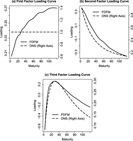
Figure 1: Example of factor loading curves: FDFM curves (solid, left axis) estimated from the period May 1985 to April 1994; pre-specified DNS curves (dashed, right axis). FDFM estimates closely resemble the shape of the DNS curves for the second and third factors, while the first FDFM factor loading curve resembles a typical yield curve shape. Dual axes are used to account for difference in scale: FDFM is represented on the left axis; DNS on the right axis.

3.2 The dynamic Nelson–Siegel model (DNS)

In the following sections we compare the FDFM with the DNS model presented in Diebold and Li (2006). Their model is composed of three factors with corresponding factor loading curves. The factor loadings are pre-specified parametric curves (see the dashed curves in Figure 1) based on financial economic theory. Let $x_{i}(t)$ denote the yield at date $i$ on a zero coupon bond of maturity $t$, then the DNS model is represented as

$$\cases{\displaystyle x_{i}(t)=\sum_{k=1}^{3}\beta_{i,k}f_{k}(t)+\varepsilon_{i}(t)\qquad\mbox{for }i=1,\ldots,n,\vspace*{2pt}\cr\displaystyle f_{1}(t)\equiv 1,\qquad f_{2}(t)\equiv\frac{1-\exp(-\alpha_{i}t)}{\alpha_{i}t},\vspace*{2pt}\cr f_{3}(t)\equiv f_{2}(2)-\exp(-\alpha_{i}t),&\vspace*{2pt}\cr\displaystyle\beta_{i,k}=c_{k}+\varphi_{k}\beta_{i-1,k}+\zeta_{i,k}\qquad\mbox{for }k=1,2,3,}$$ (21)

evaluated at maturities $t_{j}$, $j=1,\ldots,m$. The first loading curve $f_{1}(t)$ is constant and intended to represent the long-term component of yields (level); the second $f_{2}(t)$ represents a short-term component, or slope. Finally, the third loading $f_{3}(t)$ represents a mid-term component, or curvature. The parameter $\alpha_{i}$ determines the point $t^{*}(\alpha_{i})$ at which $f_{3}(t)$ achieves its maximum. While this can be estimated as a fourth factor [see, e.g., Koopman, Mallee and Van der Wel (2010)], Diebold and Li (2006) set $\alpha_{i}$ to a fixed value for all $i=1,\ldots,n$. This results in entirely predetermined, parametric curves. The specific value $\alpha=0.0609$ is determined by their definition of “mid-term” as $t=30$ months.

Estimation of the DNS model is a two-step procedure. First, time series of factor scores of $\hat{\beta}_{i,k}$ are estimated by ordinary least squares (OLS) of $x_{i}(t_{j})$ on $[1,f_{2}(t_{j}),f_{3}(t_{j})]$ for $j=1,\ldots,m$ at each time point $i=1,\ldots,n$. Second, an $\operatorname{AR}(1)$ model is fit on each series $\hat{\beta}_{i,k}$ for the purpose of forecasting $\hat{\beta}_{n+1,k}$ and ultimately $\hat{x}_{n+1}(t_{j})$ via equation (18) from Section 2.4.

3.3 Assessment

We assess the performance of the FDFM in three distinct exercises. The first two are traditional error based assessments of forecasts or within-sample predictions of yield curves or sections thereof. The final application is a combination of both forecasting and curve synthesis. Through an adaptation of the trading algorithms introduced in Bowsher and Meeks (2008), we develop trading strategies based on the forecasts of the FDFM and DNS models and assess the resulting profit generated by each.

For each of these, as a comparison, we use the DNS specification aforementioned above in Section 3.2. For the purpose of making an unbiased comparison, we use a similar formulation of our FDFM model with 3 factors following independent $\operatorname{AR}(1)$ processes. The key distinction between this FDFM model and the DNS model is that the FDFM estimates the model simultaneously: the smooth factor loading curves and the $\operatorname{AR}(1)$ parameters are estimated in a single step. In contrast, the estimation for the DNS model requires two steps given the pre-specified factor loading curves: first the factor time series are estimated; from these the $\operatorname{AR}(1)$ parameters are determined.

The key distinction between the two models raises an interesting question: How do the factor loading curves between the two models compare? Figure 1, panels (a)–(c), show an example of the factor loading curves estimated by the FDFM (solid line) for the period May 1985 through April 1994. Pictured alongside, the dashed line plots the DNS model curves. Recall the DNS motivation for the form of $f_{1}$, $f_{2}$ and $f_{3}$ was an economic argument, while the formulation of the FDFM described in Section 2 is based entirely on statistical considerations. Despite this, we see that the FDFM model is flexible enough to adapt to a specific application. Factor loading curves $f_{2}(t)$ and $f_{3}(t)$ from the FDFM assume the behavior of those from the DNS model without imposing any constraints that would force this. Thus, the FDFM inherits the economic interpretation of $f_{2}(t)$ and $f_{3}(t)$ set forth in Diebold and Li (2006). In the case of $f_{1}(t)$, the FDFM version resembles a typical yield curve shape as opposed to a constant value for DNS; however, inspecting the magnitude suggests that departure of the FDFM version from a constant value is small. Less typical yield curve shapes are usually characterized by deviations in the short and mid-term yields from the norm. This is exactly what $f_{2}(t)$, $f_{3}(t)$ and their corresponding scores capture. Thus, we consider the first factor as the mean yield, while the second and third account for short and mid-term deviations from this norm.

3.3.1 Forecast error assessment

In this section we compare the FDFM and DNS models using a rolling window of 108 months to forecast the yield curve 1, 6 or 12 months ahead. For example, for the one month ahead forecast we fit the models on the first 108 months of data and forecast the 109th month, then fit the models on the 2nd through 109th month and forecast the 110th month, etc. Yields on bonds of maturity less than three months are omitted in order to match the methodology used in Diebold and Li (2006). To compare the models, we use the mean forecast error (MFE), root mean squared forecast error (RMSFE) and mean absolute percentage error (MAPE):

$$\operatorname{MFE}_{j} = \sum_{i=1}^{r}\frac{[x_{n+h}(t_{j})-\hat{x}_{n+h}(t_{j})]}{r},$$

$$\operatorname{RMSFE}_{j} = \sqrt{\sum_{i=1}^{r}\frac{[x_{n+h}(t_{j})-\hat{x}_{n+h}(t_{j})]^{2}}{r}},$$

$$\operatorname{MAPE}_{j} = \frac{100}{r}\sum_{i=1}^{r}\frac{|x_{n+h}(t_{j})-\hat{x}_{n+h}(t_{j})|}{x_{n+h}(t_{j})},$$

where $r=84,79,73$ is the number of rolling forecasts for forecast horizon $h=1,6,12$, respectively.

A summary of the forecasting performance is shown in Table 1. For month ahead forecasts, the MFE is lower (in magnitude) with the FDFM for four out of the five displayed maturities (highlighted in bold), while RMSFE is lower for all five. For six months ahead, DNS outperforms FDFM just 2 out of five times in both MFE and RMSFE. For twelve month ahead forecasts, DNS outperforms FDFM in MFE for 3 of 5 displayed maturities. However, FDFM has lower RMSE for all 5 maturities. In terms of MAPE, the FDFM exhibits lower MAPE than DNS nearly uniformly for the displayed maturities and for 1, 6 and 12 month ahead forecasts.

Table 1: MFE, RMSFE and MAPE: 1, 6 and 12 month ahead yield curve forecast results. The better result between the two models is highlighted in bold. For 1 month ahead forecasts, the FDFM results in lower (magnitude) MFE for most maturities, but results are mixed for 6 and 12 months ahead. RMSFE and MAPE is typically lower with the FDFM for 1, 6 and 12 months ahead

	1 month ahead		6 months		12 months
Maturity	DNS	FDFM	DNS	FDFM	DNS	FDFM
	MFE
3 months	$-$0.045	0.0.026	0.0.123	0.0.172	0.0.203	0.0.257
1 year	0.0.023	0.0.035	0.0.177	0.0.168	0.0.229	0.0.215
3 years	$\bolds{-}$0.056	0.0.015	0.0.022	0.0.060	0.0.003	0.0.013
5 years	$-$0.091	$\bolds{-}$0.004	$-$0.079	$\bolds{-}$0.021	$-$0.166	$\bolds{-}$0.133
10 years	$-$0.062	$\bolds{-}$0.023	$\bolds{-}$0.139	$\bolds{-}$0.121	$\bolds{-}$0.316	$-$0.318
	RMSFE
3 months	0.0.176	0.0.164	0.0.526	0.0.535	0.0.897	0.0.867
1 year	0.0.236	0.0.233	0.0.703	0.0.727	0.0.998	0.0.967
3 years	0.0.279	0.0.274	0.0.784	0.0.775	0.1.041	0.0.947
5 years	0.0.292	0.0.277	0.0.799	0.0.772	0.1.078	0.0.953
10 years	0.0.260	0.0.250	0.0.714	0.0.697	0.1.018	0.0.921
	MAPE
3 months	.2.58	.2.50	.8.21	.8.11	12.99.	12.05.
1 year	.3.37	.3.30	10.25.	10.29.	12.70.	12.08.
3 years	.3.79	.3.77	11.68.	11.33.	14.16.	12.71.
5 years	.3.88	.3.81	11.94.	11.42.	14.93.	13.41.
10 years	.3.24	.3.24	10.49.	.9.99	14.22.	13.22.

3.3.2 Curve synthesis

Because each factor loading curve $\hat{f}_{k}(\cdot)$ is an NCS, between any two observed maturities $t_{j}$ and $t_{j+1}$, we can calculate the value for $\hat{f}_{k}(t)$. It follows, then, that between any two time series of yields $\{x_{i}(t_{j})\}_{i=1}^{n}$ and $\{x_{i}(t_{j+1})\}_{i=1}^{n}$, we are able to replicate an entire time series for the intermediate maturity $t$: $\{\hat{x}_{i}(t)\}_{i=1}^{n}$.

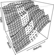
Figure 2: Example of curve synthesis: Entire time series of yields are omitted from estimation, then “filled in” using the imputation described in Section 2.4. Here, 3 consecutive maturities have been omitted, resulting in 3 missing time series corresponding to these maturities.

To illustrate this point, we use the entire data set (see introduction of Section 3), that is, use $i=1,\ldots,n=192$ months of yield data for maturities $t_{j}$, $m=18$. For both the DNS and FDFM models, we delete a set of adjacent time series from the data, estimate the model, then assess the prediction error of the predicted series in reference to the actual deleted series. Specifically, for our data matrix $\mathbf{X}_{n\times m}$ with columns $\mathbf{x}_{1},\ldots,\mathbf{x}_{m}$, we omit $l=1,\ldots,L$ consecutive columns from $\mathbf{X}$, then estimate the model on the remaining $Q\equiv m-L$ maturities. From this we compute the $L$ time series of missing data: $\hat{\mathbf{x}}_{j},\ldots,\hat{\mathbf{x}}_{j+L}$; an example for the case where $L=3$ is shown in Figure 2. For each choice of $L$, we delete a “horizontally” rolling window of width $L$ maturities and estimate the model on the remaining $Q$ maturities, $R\equiv m-L+1$ times. As an example, for $L=3$, we can estimate the models on $\mathbf{x}_{4},\ldots,\mathbf{x}_{m}$ and predict $\hat{\mathbf{x}}_{1},\ldots,\hat{\mathbf{x}}_{3}$; then estimate the models on $\mathbf{x}_{1},\mathbf{x}_{5},\ldots,\mathbf{x}_{m}$ and predict $\hat{\mathbf{x}}_{2},\ldots,\hat{\mathbf{x}}_{4}$, etc.

We examine the RMSFE for the $l$th omitted maturity of the $r$th sequence; $r=1,\ldots,R$; $l=1,\ldots,L$. Because the models are estimated based on a rolling window of maturities, for each choice of $L$ a time series $\mathbf{x}_{j}$ for yield $t_{j}$ will be estimated multiple times. Therefore, for each choice of $L$ we take the mean of the RMSFE of the predicted series for each maturity. We further average over our definitions of short ($t\in[1.5,21)$), mid ($t\in[21,36]$) and long-term ($t\in(36,120]$) horizons. Finally, we average over all maturities as a one-number summary. These results are presented in Table 2 with FDFM as a fraction of DNS. Because prediction for the FDFM model outside the range of the data is linear extrapolation, we expect these to become increasingly inaccurate as $L$ grows large. Thus, results are also presented excluding extrapolated predictions in order to better illustrate the truly functional predictions of the FDFM.

In general, as $L$ increases from 1 to 8 we see the expected decline in the performance of the FDFM model relative to DNS. In panel (a) of Table 2 the average RMSFE on short-term bonds for the FDFM remains surprisingly robust as we delete more and more maturities. On mid-term bonds, DNS results in lower prediction error when the number of deleted series reaches 5 or more. For long term, DNS more or less outperforms FDFM across the board (this trend will be echoed in Section 3.3.3). These results are similar whether or not the extrapolated results are included. Perhaps the best summary is the last column in each of panel (a) and (b) of Table 2, where, beyond 3 or 4 omitted maturities, the parametric based DNS model begins to outperform the FDFM.

Table 2: Average RMSFE; FDFM as a fraction of DNS: (a) with extrapolation (b) without extrapolation

	(a) With extrapolation				(b) Without extrapolation
Omitted	Short	Mid	Long	All	Short	Mid	Long	All
1	0.88	0.97	1.05	0.95	0.84	0.97	1.04	0.94
2	0.95	0.90	1.13	1.00	0.90	0.90	1.01	0.94
3	0.94	0.98	1.06	0.98	1.00	0.98	1.00	0.99
4	0.87	0.93	1.64	1.14	0.99	0.93	1.07	1.01
5	0.99	1.01	0.88	0.95	1.07	1.01	0.99	1.03
6	0.99	1.00	1.67	1.26	1.05	1.00	1.20	1.09
7	1.34	1.11	0.93	1.13	1.24	1.11	1.16	1.19
8	0.92	1.17	1.82	1.39	1.30	1.18	1.48	1.33

3.3.3 Portfolio-based assessment

RMSFE-type assessment providesa good diagnostic measure of forecast performance from a statistical perspective. However, as Bowsher and Meeks (2008) argued in their paper, in applied economic settings, a pure error-based assessment measure may fail to fully explain the financial implications of having used a particular model. Therefore, in this section we consider an adaptation of the profit based assessment introduced therein. By using modified versions of their three trading strategies, we create portfolios based on the model forecasts, then measure the cumulative profit of the strategy. This also serves as a good capstone exercise for our presentation of the FDFM, as it simultaneously involves both forecasting and curve synthesis: the primary uses for our model.

In each strategy we use the same rolling window of 108 months as described in Section 3.3.1 so that the trading algorithm is employed every month over the course of 84 months. Each period $i$ we create a portfolio consisting of a $1M purchase of one bond or set of bonds and a corresponding sale of another bond or set of bonds for the same amount. Therefore, the net investment per period is $0. The decision of which bond to sell and which to buy is made based on the sign of the predicted spread in their one period returns.

At time $i+1$ we cash out our portfolio and record the cumulative profit over the 84 month trading period. Denoting the yield at time $i$ of a zero coupon bond of maturity $t$ months as $x_{i}(t)$, the price of the bond at time $i$ is

$$P_{i}(t)=\exp[-tx_{i}(t)].$$ (22)

Correspondingly, the price the next period (month) is then $P_{i+1}(t-1)=\exp[-(t-1)x_{i+1}(t-1)]$ since in the month that has elapsed the maturity is reduced by, not surprisingly, one month. We denote the one period return as

$$R_{i+1}(t)=\biggl{[}\frac{P_{i+1}(t-1)}{P_{i}(t)}\biggr{]}-1,$$ (23)

and the log one period return as $r_{i+1}(t)\equiv\ln[1+R_{i+1}(t)]$. Equations (22) and (23) imply

$$r_{i+1}(t)=tx_{i}(t)-(t-1)x_{i+1}(t-1).$$ (24)

Thus, for a forecasted yield $\hat{x}_{i+1|i}(t)$ we have $\hat{r}_{i+1|i}(t)=tx_{i}(t)-(t-1)\hat{x}_{i+1|i}(t-1)$, which is a combination of both actual and forecasted yields. We use the data presented in Section 3.1 and thus are limited to a set of nonconsecutive observed maturities. Akin to Bowsher and Meeks (2008), we rely on linear interpolation of $x_{i}(t-1)$ to provide the yield for $x_{i}(t)$ and use the same random walk forecast (RW) as a benchmark by which to compare models:

$$x_{i+1}(t)=x_{i}(t)+\eta_{i+1}(t),\qquad\eta_{i+1}(t)\stackrel{{\scriptstyle\mathrm{i.i.d.}}}{{\sim}}\mathit{WN}(0,\nu^{2}),$$ (25)

with forecast $\hat{x}_{i+1|i}(t)=x_{i}(t)$.

Algorithm 1.

For this strategy, we adopt the method used in the second algorithm presented in Bowsher and Meeks (2008). Ours differs slightly since the data we use (introduced in Section 3.1) does not contain the two month maturity. Let $T=\{4,5,\ldots,13,16,\ldots,85\}$, $t_{1}$ = 4 and $t_{2,j}\in T\setminus\{4\}$; $j=1,\ldots,33$. Every period $i$ we form a portfolio of sub-portfolios with two bonds $\{t_{1},t_{2,j}\}$. Define weights $w_{j}$ as the proportion of the historical absolute excess return on portfolio $\{t_{1},t_{2,j}\}$ to the sum over all $j$ of the same:

$$w_{j}=\frac{\sum_{i}|R_{i}(t_{2,j})-R_{i}(t_{1})|}{\sum_{j}\sum_{i}|R_{i}(t_{2,j})-R_{i}(t_{1})|},$$

where $i$ spans the period January 1985 to December 1993.

To borrow some notation from Bowsher and Meeks (2008), let $d_{ij}$ represent the investment rule for the amount at time $i$ invested in each $j$th sub-portfolio. To determine the amount invested in each sub-portfolio, let

$$d_{ij}=\$1M\times w_{j}\times\operatorname{sgn}[\hat{r}_{i+1|i}(t_{2j})-\hat{r}_{i+1|i}(t_{1})].$$

We set $d_{ij}=0$ in the off chance of $\hat{r}_{i+1|i}(t_{2j})=\hat{r}_{i+1|i}(t_{1})$. Let $\pi_{i+1}$ denote the time $i+1$ profit resulting from these rules. Then

$$\pi_{i+1}=\sum_{j}d_{ij}[R_{i+1}(t_{2j})-R_{i+1}(t_{1})]\approx\sum_{j}d_{ij}[r_{i+1}(t_{2j})-r_{i+1}(t_{1})].$$

The results of this trading strategy are summarized in Table 3. Use of the FDFM model results in nearly twice the cumulative profit produced from the DNS model. Also shown is the capability of each model in successfully predicting the positive (1520) and negative (1252) actual spreads of the sub-portfolios in each period. Surprisingly, the random walk model has the greatest accuracy in predicting positive spreads (84%), as compared to the FDFM (73%) and DNS (61%) models. All three models are less accurate in the prediction of a negative spread, though RW is the worst by far (8%).

Table 3: Algorithm 1: Weighted pairs. Use of the FDFM model results in nearly twice the cumulative profit produced from the DNS model

	Profit ($\bolds{\times\$1000}$)				Directional accuracy of sub-portfolios
			Percentile		$\bolds{+}$	$\bolds{-}$
Model	Cumulative	Median	10th	90th
FDFM	1089	00.5.06	$-$101.92	149.53	1102$/$1520 (72.5%)	392$/$1252 (31.3%)
DNS	0,519	00.5.07	$-$110.77	116.02	926$/$1520 (60.9%)	538$/$1252 (43%)
RW	0$-$94	$-$10.52	$-$190.50	163.64	1274$/$1520 (83.8%)	97$/$1252 (7.7%)

Algorithm 2.

The strategy in Algorithm 1 is a fairly basic one: to use every available bond at our disposal to predict the spread between its return and a short-term bond. Our second strategy is more sophisticated by creating portfolios of an optimal pair of bonds each period $i$. Given a fixed value of $t_{1}$, we choose $t_{2i}$ to optimize the absolute spread in predicted return each trading period:

$$t_{2i}=\arg\max_{t\neq t_{1}}|\hat{r}_{i+1|i}(t)-\hat{r}_{i+1|i}(t_{1})|.$$ (26)

This is an adaption of the third algorithm presented in Bowsher and Meeks (2008). There, in a single exercise, the authors fix $t_{1}=3$ and select $t_{2i}$ according to equation (26) each trading period. Here, we examine multiple choices for $t_{1}$ and determine $t_{2i}$ according to equation (26) each trading period for each choice of fixed $t_{1}$. Because we examine multiple portfolios, we use a sparser set of maturities in this exercise than previously, though of the same range. This set is defined by the observed maturities of Section 3.1:

$$t_{1},t_{2i}\in T=\{4,7,10,13,16,19,22,25,31,37,49,61,73,85\}.$$

We perform this exercise for all choices of $t_{1}$ and $t_{2i}$ as long as $t_{1}<t_{2i}$, and compare the results. Our investment rule $d_{i}$ at time $i$ and resulting profit $\pi_{i+1}$ the next period is of a similar form to Algorithm 1:

$$d_{i} = \$1M\times\operatorname{sgn}[\hat{r}_{i+1|i}(t_{2i})-\hat{r}_{i+1|i}(t_{1})],$$

$$\pi_{i+1} = d_{i}[R_{i+1}(t_{2i})-R_{i+1}(t_{1})]\approx d_{i}[r_{i+1}(t_{2i})-r_{i+1}(t_{1})].$$

Again, we set $d_{i}=0$ whenever $\hat{r}_{i+1|i}(t_{2i})=\hat{r}_{i+1|i}(t_{1})$.

Table 4: Algorithm 2: Optimal pairs portfolio

		Profit ($\bolds{\times\$1000}$)					Profit ($\bolds{\times\$1000}$)
	$\bolds{t_{1}}$	FDFM	DNS	RW		$\bolds{t_{1}}$	FDFM	DNS	RW
Short	03	1013	3574	$-$228	Mid	21	1246	202	0680
	06	1381	2828	$-$133		24	1592	242	0070
	09	1061	1013	$-$297		30	2284	203	$-$951
	12	1873	$-$367	$-$307		36	1466	919	$-$173
	15	1519	$-$582	$-$432	Long	48	$-$361	589	0236
	18	1081	$-$481	$-$263		60	0740	339	$-$284
						72	$-$131	0$-$1	0072

The results of the strategy are shown in Table 4. When the choice of $t_{1}$ is six months or less, the DNS model generates greater cumulative profit than either of the other models. However, when the choice of $t_{1}$ is within 9 and 36 months, the FDFM consistently generates significantly greater profit than the DNS and RW models. Thus, when we are free to pick the bond that optimizes the predicted spread each period, the FDFM performs rather well, provided the maturity of the first bond is within a certain range. Our final strategy expands upon this idea.

Algorithm 3.

Because the choice of the optimal second bond can vary from one period to the next in Algorithm 2, it is not clear what a consistently good combination is. Thus, for our third strategy we consider an exploratory and exhaustive approach as a diagnostic assessment of with which combination of bonds our model excels. As such, we expand our set of bonds to include those of longer maturity:

$$t_{1},t_{2}\in T=\{4,7,10,13,16,19,22,25,31,37,49,61,73,85,97,109\}.$$

In this modification of strategy 1 from Bowsher and Meeks (2008), the portfolio is a simple one consisting of two bonds with maturities $t_{1}$ and $t_{2}$. For the duration of the strategy, these maturities remain fixed over all periods $i=1,\ldots,84$. As before, the decision at time $i$ of which bond to sell and which to buy is made based on the predicted direction of the spread in log one period returns: $d_{i}=\$1M\times\operatorname{sgn}[\hat{r}_{i+1|i}(t_{2})-\hat{r}_{i+1|i}(t_{1})]$ [we set $d_{i}=0$ whenever $\hat{r}_{i+1|i}(t_{2})=\hat{r}_{i+1|i}(t_{1})$]. This yields the time $i+1$ profit

$$\pi_{i+1}=d_{i}[R_{i+1}(t_{2})-R_{i+1}(t_{1})]\approx d_{i}[r_{i+1}(t_{2})-r_{i+1}(t_{1})].$$

We examine the cumulative profit of all combinations of this type or portfolio such that $t_{2}>t_{1}$.

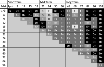
Figure 3: Algorithm 3: All combinations of portfolios for $t_{2}>t_{1}$. The model with the largest cumulative profit is displayed by the first initial of its acronym with “$+$” or “$-$” indicating positive or negative profit.

Figure 3 depicts the results of our final trading strategy. For each combination of $t_{2}>t_{1}$, the name of model with the largest cumulative profit is displayed in that cell by the first initial of its acronym (“F” for FDFM, e.g.). A “$+$” or “$-$” suffix indicates the largest profit was positive or negative, respectively.

The FDFM model typically has the greatest profit when $t_{2}\in\{30,\ldots,72\}$. These results are consistent with Sections 3.3.1 and 3.3.2: the FDFM was either comparable or better on RMSFE for forecasting and for imputation on maturities in this range. We also see a certain similarity in these results to those of Algorithm 2. Namely, that the FDFM typically outperformed the other two models when $t_{1}$ was exactly in this range.

For the longest maturities ($>72$), the DNS model results in greater profit when $t_{1}<48$. Results for other regions are mixed. Recall from Section 3.1 that in our data short and mid-term yields are typically spaced either 3 or 6 months apart, whereas long-term maturities are spaced 12 months apart. As we saw in Section 3.3.2, as the spacing between maturities increased, the FDFM model eventually broke down; it is, after all, very much a data driven model. DNS, on the other hand, maintains the same factor loading curves regardless of the data, which could explain its greater profits at long maturities.

4 Conclusion and discussion

In this paper we developed a method for modeling and forecasting functional time series. This novel approach synthesizes concepts from functional data analysis and dynamic factor modeling culminating in a functional dynamic factor model. By specifying error assumptions and smoothness conditions for functional coefficients, estimation by the Expectation Maximization algorithm results in nonparametric factor loading curves that are natural cubic splines. Thus, for a given time series of curves we can forecast entire curves as opposed to a discrete multivariate time series.

The motivating application is yield curve forecasting, where existing approaches typically exhibit a trade-off of consistency-with-economic-theory and goodness of fit. However, through multiple forecasting exercises we show that our model satisfies both of these criteria. A further online supplement underscores these results and also showcases the model’s viability to settings well outside of economics and yield curve forecasting and where a prior theory does not exist. Indeed, this exciting new class of models is fertile for further development and application.

The present paper focuses on yields of zero coupon bonds. A particularly interesting direction for future research is the extension of our modeling framework to yields implied by commodities that include convenience factors. For example, see Casassus and Collin-Dufresne (2005) and Chua et al. (2008). A potential difficulty in this regard is the consistent control of multiple parameters: the commodity, the maturity and the liquidity of said maturity, for example. Another interesting direction of research is to develop nonlinear time series models for functional data; existing approaches for nonlinear univariate time series modeling [see Fan and Yao (2003), Section 1.5.4] may be helpful for that purpose.

References

- Basilevsky (1994) {bbook}[mr] \bauthor\bsnmBasilevsky, \bfnmAlexander\binitsA. (\byear1994). \btitleStatistical Factor Analysis and Related Methods: Theory and Applications. \bpublisherWiley, \baddressNew York. \biddoi=10.1002/9780470316894, mr=1277625 \bptokimsref \endbibitem
- Besse, Cardot and Stephenson (2000) {barticle}[author] \bauthor\bsnmBesse, \bfnmPhilippe C.\binitsP. C., \bauthor\bsnmCardot, \bfnmHerve\binitsH. and \bauthor\bsnmStephenson, \bfnmDavid B.\binitsD. B. (\byear2000). \btitleAutoregressive forecasting of some functional climatic variations. \bjournalScand. J. Stat. \bvolume27 \bpages673–687. \bptokimsref \endbibitem
- Bowsher and Meeks (2008) {barticle}[mr] \bauthor\bsnmBowsher, \bfnmClive G.\binitsC. G. and \bauthor\bsnmMeeks, \bfnmRoland\binitsR. (\byear2008). \btitleThe dynamics of economic functions: Modeling and forecasting the yield curve. \bjournalJ. Amer. Statist. Assoc. \bvolume103 \bpages1419–1437. \biddoi=10.1198/016214508000000922, issn=0162-1459, mr=2504199 \bptokimsref \endbibitem
- Casassus and Collin-Dufresne (2005) {barticle}[author] \bauthor\bsnmCasassus, \bfnmJ.\binitsJ. and \bauthor\bsnmCollin-Dufresne, \bfnmP.\binitsP. (\byear2005). \btitleStochastic convenience yield implied from commodity futures and interest rates. \bjournalJ. Finance \bvolume60 \bpages2283–2331. \bptokimsref \endbibitem
- Chua et al. (2008) {barticle}[author] \bauthor\bsnmChua, \bfnmC. T.\binitsC. T., \bauthor\bsnmFoster, \bfnmD.\binitsD., \bauthor\bsnmRamaswamy, \bfnmK.\binitsK. and \bauthor\bsnmStine, \bfnmR.\binitsR. (\byear2008). \btitleA dynamic model for the forward curve. \bjournalReview of Financial Studies \bvolume21 \bpages265–310. \bptokimsref \endbibitem
- Cox, Ingersoll and Ross (1985) {barticle}[mr] \bauthor\bsnmCox, \bfnmJohn C.\binitsJ. C., \bauthor\bsnmIngersoll, \bfnmJonathan E.\binitsJ. E. \bsuffixJr. and \bauthor\bsnmRoss, \bfnmStephen A.\binitsS. A. (\byear1985). \btitleA theory of the term structure of interest rates. \bjournalEconometrica \bvolume53 \bpages385–407. \biddoi=10.2307/1911242, issn=0012-9682, mr=0785475 \bptokimsref \endbibitem
- Dempster, Laird and Rubin (1977) {barticle}[mr] \bauthor\bsnmDempster, \bfnmA. P.\binitsA. P., \bauthor\bsnmLaird, \bfnmN. M.\binitsN. M. and \bauthor\bsnmRubin, \bfnmD. B.\binitsD. B. (\byear1977). \btitleMaximum likelihood from incomplete data via the EM algorithm. \bjournalJ. Roy. Statist. Soc. Ser. B \bvolume39 \bpages1–38. \bidissn=0035-9246, mr=0501537 \bptnotecheck related\bptokimsref \endbibitem
- Diebold and Li (2006) {barticle}[mr] \bauthor\bsnmDiebold, \bfnmFrancis X.\binitsF. X. and \bauthor\bsnmLi, \bfnmCanlin\binitsC. (\byear2006). \btitleForecasting the term structure of government bond yields. \bjournalJ. Econometrics \bvolume130 \bpages337–364. \biddoi=10.1016/j.jeconom.2005.03.005, issn=0304-4076, mr=2211798 \bptokimsref \endbibitem
- Diebold, Rudebusch and Aruoba (2006) {barticle}[mr] \bauthor\bsnmDiebold, \bfnmFrancis X.\binitsF. X., \bauthor\bsnmRudebusch, \bfnmGlenn D.\binitsG. D. and \bauthor\bsnmAruoba, \bfnmS. Borağan\binitsS. B. (\byear2006). \btitleThe macroeconomy and the yield curve: A dynamic latent factor approach. \bjournalJ. Econometrics \bvolume131 \bpages309–338. \biddoi=10.1016/j.jeconom.2005.01.011, issn=0304-4076, mr=2276003 \bptokimsref \endbibitem
- Duffee (2002) {barticle}[author] \bauthor\bsnmDuffee, \bfnmG.\binitsG. (\byear2002). \btitleTerm premia and interest rate forecasts in affine models. \bjournalJ. Finance \bvolume57 \bpages405–443. \bptokimsref \endbibitem
- Duffie and Kan (1996) {barticle}[author] \bauthor\bsnmDuffie, \bfnmD.\binitsD. and \bauthor\bsnmKan, \bfnmR.\binitsR. (\byear1996). \btitleA yield factor model of interest rates. \bjournalMath. Finance \bvolume6 \bpages379–406. \bptokimsref \endbibitem
- Engle and Watson (1981) {barticle}[author] \bauthor\bsnmEngle, \bfnmRobert\binitsR. and \bauthor\bsnmWatson, \bfnmMark\binitsM. (\byear1981). \btitleA one-factor multivariate time series model of metropolitan wage rates. \bjournalJ. Amer. Statist. Assoc. \bvolume78 \bpages774–781. \bptokimsref \endbibitem
- Fama and Bliss (1987) {barticle}[author] \bauthor\bsnmFama, \bfnmE.\binitsE. and \bauthor\bsnmBliss, \bfnmR.\binitsR. (\byear1987). \btitleThe information in long-maturity forward rates. \bjournalAmerican Economic Review \bvolume77 \bpages680–692. \bptokimsref \endbibitem
- Fan and Yao (2003) {bbook}[mr] \bauthor\bsnmFan, \bfnmJianqing\binitsJ. and \bauthor\bsnmYao, \bfnmQiwei\binitsQ. (\byear2003). \btitleNonlinear Time Series: Nonparametric and Parametric Methods. \bpublisherSpringer, \baddressNew York. \biddoi=10.1007/b97702, mr=1964455 \bptnotecheck year\bptokimsref \endbibitem
- Geweke and Singleton (1981) {barticle}[mr] \bauthor\bsnmGeweke, \bfnmJohn F.\binitsJ. F. and \bauthor\bsnmSingleton, \bfnmKenneth J.\binitsK. J. (\byear1981). \btitleMaximum likelihood “confirmatory” factor analysis of economic time series. \bjournalInternat. Econom. Rev. \bvolume22 \bpages37–54. \biddoi=10.2307/2526134, issn=0020-6598, mr=0614346 \bptokimsref \endbibitem
- Green and Silverman (1994) {bbook}[mr] \bauthor\bsnmGreen, \bfnmP. J.\binitsP. J. and \bauthor\bsnmSilverman, \bfnmB. W.\binitsB. W. (\byear1994). \btitleNonparametric Regression and Generalized Linear Models: A Roughness Penalty Approach. \bseriesMonographs on Statistics and Applied Probability \bvolume58. \bpublisherChapman & Hall, \baddressLondon. \bidmr=1270012 \bptokimsref \endbibitem
- Hays, Shen and Huang (2012) {bmisc}[author] \bauthor\bsnmHays, \bfnmS.\binitsS., \bauthor\bsnmShen, \bfnmH.\binitsH. and \bauthor\bsnmHuang, \bfnmJ. Z.\binitsJ. Z. (\byear2012). \bhowpublishedSupplement to “Functional dynamic factor models with application to yield curve forecasting”. DOI:\doiurl10.1214/12-AOAS551SUPP. \bptokimsref \endbibitem
- Heath, Jarrow and Morton (1992) {barticle}[author] \bauthor\bsnmHeath, \bfnmD.\binitsD., \bauthor\bsnmJarrow, \bfnmR.\binitsR. and \bauthor\bsnmMorton, \bfnmA.\binitsA. (\byear1992). \btitleBond pricing and the term structure of interest rates: A new methodology for contingent claims valuation. \bjournalEconometrica \bvolume60 \bpages77–105. \bptokimsref \endbibitem
- Hull and White (1990) {barticle}[author] \bauthor\bsnmHull, \bfnmJ.\binitsJ. and \bauthor\bsnmWhite, \bfnmA.\binitsA. (\byear1990). \btitlePricing interest–rate–derivative securities. \bjournalReview of Financial Studies \bvolume3 \bpages573–592. \bptokimsref \endbibitem
- Hyndman and Shang (2009) {barticle}[mr] \bauthor\bsnmHyndman, \bfnmRob J.\binitsR. J. and \bauthor\bsnmShang, \bfnmHan Lin\binitsH. L. (\byear2009). \btitleForecasting functional time series. \bjournalJ. Korean Statist. Soc. \bvolume38 \bpages199–211. \biddoi=10.1016/j.jkss.2009.06.002, issn=1226-3192, mr=2750314 \bptokimsref \endbibitem
- Judge (1985) {bbook}[author] \bauthor\bsnmJudge, \bfnmGeorge G.\binitsG. G. (\byear1985). \btitleThe Theory and Practice of Econometrics. \bpublisherWiley, \baddressNew York. \bptokimsref \endbibitem
- Koopman, Mallee and Van der Wel (2010) {barticle}[mr] \bauthor\bsnmKoopman, \bfnmSiem Jan\binitsS. J., \bauthor\bsnmMallee, \bfnmMax I. P.\binitsM. I. P. and \bauthor\bparticleVan der \bsnmWel, \bfnmMichel\binitsM. (\byear2010). \btitleAnalyzing the term structure of interest rates using the dynamic Nelson–Siegel model with time-varying parameters. \bjournalJ. Bus. Econom. Statist. \bvolume28 \bpages329–343. \biddoi=10.1198/jbes.2009.07295, issn=0735-0015, mr=2723603 \bptokimsref \endbibitem
- Molenaar (1985) {barticle}[author] \bauthor\bsnmMolenaar, \bfnmPeter C. M.\binitsP. C. M. (\byear1985). \btitleA dynamic factor model for the analysis of multivariate time series. \bjournalPsychometrika \bvolume50 \bpages181–202. \bptokimsref \endbibitem
- Nelson and Siegel (1987) {barticle}[author] \bauthor\bsnmNelson, \bfnmC. R.\binitsC. R. and \bauthor\bsnmSiegel, \bfnmA. F.\binitsA. F. (\byear1987). \btitleParsimonious modeling of yield curves. \bjournalJournal of Business \bvolume60 \bpages473–489. \bptokimsref \endbibitem
- Peña and Box (1987) {barticle}[mr] \bauthor\bsnmPeña, \bfnmDaniel\binitsD. and \bauthor\bsnmBox, \bfnmGeorge E. P.\binitsG. E. P. (\byear1987). \btitleIdentifying a simplifying structure in time series. \bjournalJ. Amer. Statist. Assoc. \bvolume82 \bpages836–843. \bidissn=0162-1459, mr=0909990 \bptokimsref \endbibitem
- Peña and Poncela (2004) {barticle}[mr] \bauthor\bsnmPeña, \bfnmDaniel\binitsD. and \bauthor\bsnmPoncela, \bfnmPilar\binitsP. (\byear2004). \btitleForecasting with nonstationary dynamic factor models. \bjournalJ. Econometrics \bvolume119 \bpages291–321. \biddoi=10.1016/S0304-4076(03)00198-2, issn=0304-4076, mr=2057102 \bptokimsref \endbibitem
- Press et al. (1992) {bbook}[mr] \bauthor\bsnmPress, \bfnmWilliam H.\binitsW. H., \bauthor\bsnmTeukolsky, \bfnmSaul A.\binitsS. A., \bauthor\bsnmVetterling, \bfnmWilliam T.\binitsW. T. and \bauthor\bsnmFlannery, \bfnmBrian P.\binitsB. P. (\byear1992). \btitleNumerical Recipes in FORTRAN: The Art of Scientific Computing, \bedition2nd ed. \bpublisherCambridge Univ. Press, \baddressCambridge. \bidmr=1196230 \bptokimsref \endbibitem
- Ramsay and Silverman (2002) {bbook}[mr] \bauthor\bsnmRamsay, \bfnmJ. O.\binitsJ. O. and \bauthor\bsnmSilverman, \bfnmB. W.\binitsB. W. (\byear2002). \btitleApplied Functional Data Analysis: Methods and Case Studies. \bpublisherSpringer, \baddressNew York. \biddoi=10.1007/b98886, mr=1910407 \bptokimsref \endbibitem
- Ramsay and Silverman (2005) {bbook}[mr] \bauthor\bsnmRamsay, \bfnmJ. O.\binitsJ. O. and \bauthor\bsnmSilverman, \bfnmB. W.\binitsB. W. (\byear2005). \btitleFunctional Data Analysis, \bedition2nd ed. \bpublisherSpringer, \baddressNew York. \bidmr=2168993 \bptokimsref \endbibitem
- Shen (2009) {barticle}[mr] \bauthor\bsnmShen, \bfnmHaipeng\binitsH. (\byear2009). \btitleOn modeling and forecasting time series of smooth curves. \bjournalTechnometrics \bvolume51 \bpages227–238. \biddoi=10.1198/tech.2009.08100, issn=0040-1706, mr=2751069 \bptokimsref \endbibitem
- Vasicek (1977) {barticle}[author] \bauthor\bsnmVasicek, \bfnmO.\binitsO. (\byear1977). \btitleAn equilibrium characterization of the term structure. \bjournalJournal Financial Economics \bvolume5 \bpages177–188. \bptokimsref \endbibitem