Simultaneous Localization and Mapping Problem in Wireless Sensor Networks

Abstract

Mobile device localization in wireless sensor networks is a challenging task. It has already been addressed when the WiFI propagation maps of the access points are modeled deterministically. However, this procedure does not take into account the environmental dynamics and also assumes an offline human training calibration. In this paper, the maps are made of an average indoor propagation model combined with a perturbation field which represents the influence of the environment. This perturbation field is embedded with a prior distribution. The device localization is dealt with using Sequential Monte Carlo methods and relies on the estimation of the propagation maps. This inference task is performed online, i.e. using the observations sequentially, with a recently proposed online Expectation Maximization based algorithm. The performance of the algorithm are illustrated through Monte Carlo experiments.

I Introduction

Wireless sensor networks [1] generally consist of a data acquisition network and a data distribution network, monitored and controlled by a management center. These networks have many applications such as environmental monitoring ([2]) or target tracking ([3, 4, 5]). In this paper, we consider a WiFi communication network made up of a mobile device (such as a hand held mobile computer or a smartphone), a server and WiFi access points (APs). We are interested in the estimation of the localization of the mobile device in the environment using the signal strength of the surrounding APs. The mobile device collects the power of the signals and sends the data to the server which uses them to build an estimator of the device’s position. The key step to provide such an estimator is to understand the behaviour of the WiFi signal strength for different positions in the environment. However, predicting the propagation of WiFi signals in an indoor environment is challenging since they are subject to many perturbations (e.g. shadowing, reflection…).

Two main techniques exist to approximate the WiFi signal propagation map of each AP: the first ones use deterministic models based on the localization and characteristics of the surrounding APs as well as the localization of the obstacles involved in the environment, see for instance [6]. Other famous techniques are based on a previous hand made offline training phase in which a human operator performs a site survey by measuring the received signal strength indicator (RSSI) from different APs at some fixed sampled points, see [4, 7]. However, representing the indoor propagation map using a deterministic model is challenging since several obstacles cannot be taken into account. On the contrary, the site survey method allows to build an accurate estimation of the signal strength, but only for a finite number of points. Nevertheless, [8] provides a method to extend these measures to the entire map using Gaussian processes techniques.

In this paper, we propose an estimation method that does not require any calibration procedure. The propagation maps are estimated online (i.e. without storing the observations) using the data sent by the mobile device. Any modification in the way the WiFi signals propagate inside the environment (due to new obstacles for instance) affects the data sent by the mobile device. Then, while these changes deteriorate the accuracy of localization systems using fixed estimators of the propagation maps, our system learns these changes by taking them into account in the construction of our map estimators. Thus, as illustrated in Section V-B, the accuracy of our localization method improves with time instead of degrading.

A semiparametric statistical model is used: the propagation maps are made of a parametric average indoor model in addition to a non parametric perturbation field. This model combines a prior knowledge on the signal propagation with random perturbations due to the obstacles. Based on the data collected by the mobile device, parameters and perturbation field estimators can be defined. We simultaneously provide an estimator for the device position. The procedure relies on an online Expectation-Maximization (EM) based algorithm for the estimation of the propagation maps and on particle filtering for the estimation of the device position.

The structure of this paper is the following. Section II describes the model and defines the notations. Section III presents the online EM algorithm and Section IV gives a general algorithm for online inference in our Simultaneous localization and Mapping (SLAM) problem. Section V illustrates this algorithm with numerical experiments.

II Model and assumption

Let $\{X_{t}\}_{t\geq 1}$ be the cartesian coordinates of the mobile device in a two-dimensional compact space. This continuous environment is discretized into a finite grid map, denoted by $\mathcal{C}$, for purposes of numerical computation. It is assumed that $\{X_{t}\}_{t\geq 1}$ is a Markov chain taking values in $\mathcal{C}$ with initial distribution $\nu$ and Markov transition matrix given, for all $(x,x^{\prime})\in\mathcal{C}^{2}$, by

$$q_{x,x^{\prime}}\propto\mathrm{e}^{-\|x-x^{\prime}\|^{2}/a}\;,$$ (1)

where $a\in\mathbb{R}_{+}^{\star}$ depends on the average speed of the mobile and is assumed to be known and $\|\cdot\|$ denotes the usual euclidean norm in $\mathbb{R}^{2}$. Let $B$ be the number of APs, $|\mathcal{C}|$ be the cardinality of $\mathcal{C}$ and $F^{\star}$ be the $B\times|\mathcal{C}|$ matrix where $F^{\star}_{j,x}$ is the $j$-th AP expected signal strength at position $x$. At each time step $t$, the mobile device measures and sends to the server the observation $Y_{t}$ taking values in $\mathbb{R}^{B}$. For all $t\geq 0$, the observation $Y_{t}$ is given by

$$Y_{t}\stackrel{{\scriptstyle\mathrm{def}}}{{=}}F^{\star}_{.,X_{t}}+\varepsilon_{t}\;,$$ (2)

where $F^{\star}_{.,X_{t}}\stackrel{{\scriptstyle\mathrm{def}}}{{=}}\{F^{\star}_{j,X_{t}}\}_{j=1}^{B}$ and where $\{\varepsilon_{t}\}_{t\geq 0}$ is a sequence of i.i.d Gaussian random vectors, independent from $\{X_{t}\}_{t\geq 1}$, with mean $0$ and covariance matrix $\Sigma\stackrel{{\scriptstyle\mathrm{def}}}{{=}}\sigma^{\star,2}I_{B}$ ($I_{B}$ is the identity matrix of size $B\times B$).

The position of the $B$ APs are assumed to be known and denoted by $\{O_{j}\}_{j=1}^{B}$. In order to take into account the perturbations in the signal propagation (due to the fact that radio waves are prone to shadowing, reflections and so on), we propose the following decomposition of $F^{\star}$: for all $x\in\mathcal{C}$ and all $j\in\{1,\cdots,B\}$,

$$F^{\star}_{j,x}\stackrel{{\scriptstyle\mathrm{def}}}{{=}}\mu^{\star}_{j,x}+\delta^{\star}_{j,x}\;.$$ (3)

For any $B\times\mathbb{R}^{|\mathcal{C}|}$ matrix $A$, we use the shorthand notation $A_{j}$ for the vector $\{A_{j,x}\}_{x\in\mathcal{C}}$. For any $j\in\{1,\cdots,B\}$, $\mu^{\star}_{j}$ is the average indoor propagation and is such that for all $x\in\mathcal{C}$, $\mu^{\star}_{j,x}$ only depends on the distance between $x$ and $O_{j}$. In the sequel, we use the so-called Friis transmission equation, see [9], given by,

$$\mu^{\star}_{j,x}\stackrel{{\scriptstyle\mathrm{def}}}{{=}}c^{\star}_{1,j}+c^{\star}_{2,j}\log\left\|x-O_{j}\right\|\;,$$ (4)

where $c^{\star}_{1,j}$ and $c^{\star}_{2,j}$ are parameters depending on the environment and $\log$ is the logarithm to the base e.

$\delta^{\star}_{j}$ is an additive term due to random perturbations such as walls effects (a similar model of WiFi propagation maps using Gaussian processes can be found in [8]). It is assumed that the parameters $\{\delta^{\star}_{j}\}_{j=1}^{B}$ are embedded with the prior distribution $\pi$ given, for any $\delta\in\mathbb{R}^{B.|\mathcal{C}|}$, by

$$\pi(\delta)\propto\exp\left\{-\frac{1}{2}\sum_{j=1}^{B}\delta_{j}^{T}\Sigma_{j}^{-1}\delta_{j}\right\}\;,$$

where $\Sigma_{j}$ is assumed to be known and where, for any matrix $A$, $A^{T}$ denotes the transpose of A. Figure (1) represents $\delta^{\star}_{j}$ (sampled from $\pi$) and the functions $\mu^{\star}_{j}$ and $F^{\star}_{j}$, defined on the grid $\mathcal{C}=\left\{0,\ldots,30\right\}\times\left\{0,\ldots,30\right\}$. The parameters used in this figure are $O_{j}=(15,15)$, and $c^{\star}_{1,j}$, $c^{\star}_{2,j}$ and $\Sigma_{j}$ are given in Section V, their values were calibrated after a measurement campaign in an office environment.

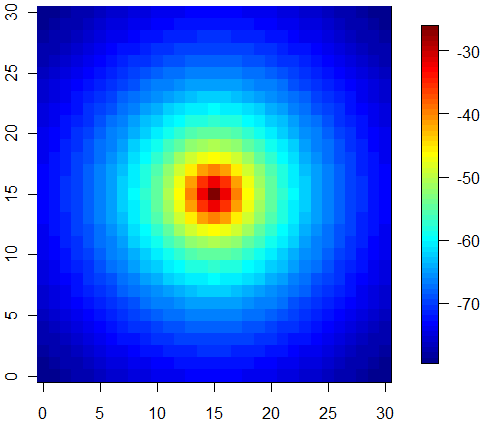
(a) $\mu_{j}^{\star}$.

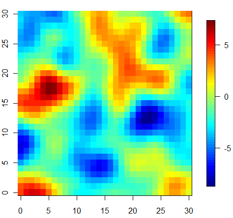
(b) $\delta_{j}^{\star}$.

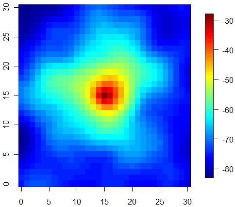
(c) $F_{j}^{\star}=\mu_{j}^{\star}+\delta_{j}^{\star}$.

Figure 1: Example of $\delta_{j}^{\star}$ (sampled from $\pi$) and spatial representations of the functions $\mu_{j}^{\star}$ and $F_{j}^{\star}=\mu_{j}^{\star}+\delta_{j}^{\star}$ (in $dBm$)

In the sequel, we write $\theta^{\star}\stackrel{{\scriptstyle\mathrm{def}}}{{=}}(c^{\star}_{1},\ c^{\star}_{2},\ \delta^{\star},\ \sigma^{\star,2})$, where $c^{\star}_{1}\stackrel{{\scriptstyle\mathrm{def}}}{{=}}\{c^{\star}_{1,j}\}_{j=1}^{B}$, $c^{\star}_{2}\stackrel{{\scriptstyle\mathrm{def}}}{{=}}\{c^{\star}_{2,j}\}_{j=1}^{B}$ and $\delta^{\star}\stackrel{{\scriptstyle\mathrm{def}}}{{=}}\{\delta^{\star}_{j}\}_{j=1}^{B}$. For any $x\in\mathcal{C}$, the distribution of $Y_{t}$ conditionally to $X_{t}=x$ has a density with respect to the Lebesgue measure on $\mathbb{R}^{B}$ given, for all $y\stackrel{{\scriptstyle\mathrm{def}}}{{=}}(y_{1},\cdots,y_{B})\in\mathbb{R}^{B}$, by

$$g_{\theta^{\star}}(x,y)\stackrel{{\scriptstyle\mathrm{def}}}{{=}}\dfrac{1}{\sqrt{2\pi\sigma^{\star,2}}^{B}}\prod_{j=1}^{B}\exp\left\{-\dfrac{1}{2\sigma^{\star,2}}|y_{j}-F^{\star}_{j,x}|^{2}\right\}\;.$$

Therefore, $\{X_{t}\}_{t\geq 0}$ is the hidden process of a hidden Markov model observed through the process $\{Y_{t}\}_{t\geq 0}$. The estimation of the mobile device’s position $X_{t}$ relies on the knowledge of the map $F^{\star}$. The observations $\{Y_{t}\}_{t\geq 1}$ are used to estimate simultaneously the mobile device’s position and $\theta^{\star}$. This simultaneous localization and mapping problem may be seen as an instance of inference in hidden Markov models. For any positive integer $n$, any observation set $(y_{1},\ldots,y_{n})$, shortly denoted by $y_{1:n}$ and any parameter $\theta=(c_{1},c_{2},\delta,\sigma^{2})$, the likelihood of the observations $L_{\theta}(y_{1:n})$ is given by:

$$L_{\theta}(y_{1:n})\stackrel{{\scriptstyle\mathrm{def}}}{{=}}\sum\limits_{x_{1:n}\in\mathcal{C}^{n}}\nu(x_{1})g_{\theta}(x_{1},y_{1})\prod\limits_{t=2}^{n}q(x_{t-1},x_{t})g_{\theta}(x_{t},y_{t})\;.$$ (5)

Let $n$ be a positive integer and $Y_{1:n}$ be a set of observations, we set as the estimator of $\theta^{\star}$, the maximum a posteriori estimator defined as $\mathrm{argmax}_{\theta}\,n^{-1}\ell_{\theta}(Y_{1:n})$, where:

$$\ell_{\theta}(Y_{1:n})\stackrel{{\scriptstyle\mathrm{def}}}{{=}}\log L_{\theta}(Y_{1:n})+\log\pi(\delta)\;.$$ (6)

The next section provides a description of the EM algorithm and of online EM algorithms for the computation of maximum likelihood estimators (without the penalty term). In Section IV, we explain how such techniques can be used in our framework.

III Online EM

The EM algorithm is a well-known iterative algorithm to perform maximum likelihood estimation in hidden Markov models [10]. Each iteration of this algorithm consists in a E-step where the expectation of the complete data log-likelihood (log of the joint distribution of the states and the observations) conditionally to the observations is computed; and a M-step, which updates the parameter estimate.

Let $Y_{1:n}$ be a fixed set of observations and $\hat{\theta}$ be the current parameter estimate.

1. The E-step consists in evaluating the conditional expectation

   $$Q_{\hat{\theta}}(Y_{1:n};\theta)=\mathbb{E}_{\hat{\theta}}\left[\frac{1}{n}\log p_{\theta}(X_{1:n},Y_{1:n})\middle|Y_{1:n}\right]\;,$$ (7)

   where $\log p_{\theta}(X_{1:n},Y_{1:n})$ is the complete data log-likelihood and $\mathbb{E}_{\hat{\theta}}\left[\cdot\middle|Y_{1:n}\right]$ is the conditional expectation given $Y_{1:n}$ when the parameter’s value is $\hat{\theta}$.

2. The M-step updates the current value $\hat{\theta}$ taking the parameter $\theta$ maximizing (7).

The model presented in Section II belongs to the curved exponential family: there exist functions $S:\mathbb{X}^{2}\times\mathbb{Y}\to\mathcal{S}\subset\mathbb{R}^{d}$, $\phi:\Theta\to\mathbb{R}$ and $\psi:\Theta\to\mathbb{R}^{d}$ such that

$$\log q(x,x^{\prime})+\log g_{\theta}(x^{\prime},y)=\phi(\theta)+\left\langle S(x,x,^{\prime},y),\psi(\theta)\right\rangle\;,$$

where $\left\langle\cdot,\cdot\right\rangle$ denotes the scalar product on $\mathbb{R}^{d}$. Moreover, there exists a continuous function $\bar{\theta}:\mathcal{S}\to\Theta$ s.t. for any $s\in\mathcal{S}$,

$$\bar{\theta}(s)=\mathrm{argmax}_{\theta\in\Theta}\;\left\{\phi(\theta)+\left\langle s,\psi(\theta)\right\rangle\right\}\;.$$

In this case the intermediate quantity defined by (7) can be written

$$Q_{\hat{\theta}}(Y_{1:n};\theta)=\phi(\theta)\\ +\left\langle\mathbb{E}_{\hat{\theta}}\left[\frac{1}{n}\sum_{t=1}^{n}S(X_{t-1},X_{t},Y_{t})\middle|Y_{1:T}\right],\psi(\theta)\right\rangle\;.$$ (8)

Therefore, the E-steps amounts to computing only one conditional expectation $\mathbb{E}_{\hat{\theta}}\left[\frac{1}{n}\sum_{t=1}^{n}S(X_{t-1},X_{t},Y_{t})\middle|Y_{1:n}\right]$ when the current parameter’s value is $\hat{\theta}$. The M-step relies simply on the evaluation of $\bar{\theta}$ at this conditional expectation. This two steps process is repeated till convergence. However, when the observations are obtained sequentially or when the E-step relies on a large data set, the EM algorithm might become impractical. Online variants of the EM algorithm have been proposed to obtain parameter estimates each time a new observation is available. In the case of independent and identically distributed (i.i.d.) observations, [11] proposed the first EM based online algorithm. The E-step amounts to computing intermediate quantities known as sufficient statistics (see below for a explicit definition) and [11] proposed to replace these computations by a stochastic approximation step. When both the observations and the states take a finite number of values (resp. when the state-space is finite) an online EM-based algorithm was proposed by [12] (resp. by [13]). These algorithms combine an online approximation of the filtering distributions of the hidden states and a stochastic approximation step to compute an online approximation of the sufficient statistics. This has been extended to the case of general state-space models with Sequential Monte Carlo algorithms (see [14], [15] and [16]). More recently, [17] proposed a block online algorithm in which the parameter estimate is kept fixed on block of observations. The parameter’s update then occurs at the end of each block.

In this paper, we use the online variant of the EM algorithm introduced in [17] to perform the parameter estimation and to solve the localization problem presented above. This algorithm, called the Block Online EM (BOEM) algorithm relies on the ability to compute sequentially quantities of the form:

$$\mathsf{S}_{n,\tau}(\theta)\stackrel{{\scriptstyle\mathrm{def}}}{{=}}\mathbb{E}_{\theta}\left[\frac{1}{\tau}\sum_{t=1}^{\tau}S(X_{t+n-1},X_{t+n},Y_{t+n})\middle|Y_{n:n+\tau}\right]\;.$$

Such quantities are called sufficient statistics. The BOEM algorithm uses a sequence of block-sizes $\{\tau_{k}\}_{k\geq 0}$. Define $T_{0}\stackrel{{\scriptstyle\mathrm{def}}}{{=}}0$ and, for any $k\geq 0$, $T_{k}\stackrel{{\scriptstyle\mathrm{def}}}{{=}}\sum_{i=1}^{k}\tau_{i}$. Let $k$ be a positive integer. Within each block of observations $Y_{T_{k}+1:T_{k+1}}$, the parameter’s value $\widehat{\theta}_{k}$ is kept fixed and the sufficient statistic $\mathsf{S}_{T_{k},\tau_{k+1}}(\widehat{\theta}_{k})$ is computed sequentially. The estimate $\widehat{\theta}_{k+1}$ is computed at the end of the block $Y_{T_{k}+1:T_{k+1}}$ through the evaluation of the function $\bar{\theta}$.

Unlike the traditional use of the EM algorithm where the conditional expectations are computed using forward-backward techniques, [13], [15] and [17] rely on recursive computations of the conditional expectations. Indeed, let $\phi_{n,\theta}$ denotes the filtering distribution of $X_{n}$ given the observations $Y_{1:n}$ when the parameter’s value is $\theta$:

$$\forall x\in\mathbb{X}\;,\;\phi_{n,\theta}(x)=P_{\theta}\left(X_{n}=x|Y_{1:n}\right)\;.$$

Following [13, 15], defining for all $x\in\mathbb{X}$ and all $\theta\in\Theta$,

$$\rho_{n,\theta}(x)=\mathbb{E}_{\theta}\left[\frac{1}{n}\sum_{t=1}^{n}S(X_{t-1},X_{t},Y_{t})\middle|Y_{1:n},\ X_{n}=x\right]\;,$$

we have,

$$\mathbb{E}_{\theta}\left[\frac{1}{n}\sum_{t=1}^{n}S(X_{t-1},X_{t},Y_{t})\middle|Y_{1:n}\right]=\sum_{x\in C}\phi_{n,\theta}(x)\rho_{n,\theta}(x)\;.$$

Proposition 1 of [13] illustrates the usefulness of this decomposition.

Proposition 1 (of [13]).

 

Initialisation:
For all $x\in\mathcal{C}$ and all $\theta\in\Theta$,

$$\phi_{1,\theta}(x) = \frac{\nu(x)g_{\theta}(x,Y_{1})}{\sum\limits_{x^{\prime}\in\mathcal{C}}\nu(x^{\prime})g_{\theta}(x^{\prime},Y_{1})}\;,$$

$$\rho_{1,\theta}(x) = 0\;.$$

Recursion:
For all $t\geq 2$ and all $x\in\mathcal{C}$,

$$\phi_{t,\theta}(x) = \frac{\sum\limits_{x^{\prime}\in\mathcal{C}}\phi_{t-1,\theta}(x^{\prime})q(x^{\prime}x)g_{\theta}(x,Y_{t})}{\sum\limits_{(x^{\prime},x^{\prime\prime})\in\mathcal{C}^{2}}\phi_{t-1,\theta}(x^{\prime})q(x^{\prime}x^{\prime\prime})g_{\theta}(x^{\prime\prime},Y_{t})}\;,$$ (9)

$$\rho_{t,\theta}(x) = \sum\limits_{x^{\prime}\in\mathcal{C}}\bigg{\{}\frac{1}{t}s(x^{\prime},x,Y_{t})+$$

$$\left(1-\frac{1}{t}\right)\rho_{t-1,\theta}(x^{\prime})\bigg{\}}.\frac{\phi_{t-1,\theta}(x^{\prime})q(x^{\prime},x)}{\sum\limits_{x^{\prime\prime}\in\mathcal{C}}\phi_{t-1,\theta}(x^{\prime\prime})q(x^{\prime\prime},x)}\;.$$

Except in simple models (linear Gaussian models and finite state-space HMM), this algorithm requires forward computations which are not available in closed form and which have to be approximated, e.g. using sequential Monte Carlo methods (see [14, 15]). In this case, $\phi_{t,\theta}$ is approximated by weighted samples $\{\widehat{\xi}_{t}^{p},\widehat{\omega}_{t}^{p}\}_{p=1}^{N}$ such that $\widehat{\phi}_{t,\theta}(x)=\sum\limits_{p=1}^{N}\widehat{\omega}_{t}^{p}\delta_{\xi_{t}^{p}}(x)$. In the sequel, $\{\widehat{\xi}_{t}^{p}\}_{p=1}^{N}$ will be referred to as the particle set at time step $t$. Plugging this approximation in (1) yields:

$$\rho_{t}^{p}=\sum_{\ell=1}^{N}\widehat{\omega}_{t-1}^{\ell}q(\widehat{\xi}_{t-1}^{\ell},\widehat{\xi}_{t}^{p})\times\frac{\frac{1}{t}s(\widehat{\xi}_{t-1}^{\ell},\widehat{\xi}_{t}^{p},Y_{t})+(1-\frac{1}{t})\rho_{t-1}^{\ell}}{\sum_{\ell=1}^{N}\widehat{\omega}_{t-1}^{\ell}q(\widehat{\xi}_{t-1}^{\ell},\widehat{\xi}_{t}^{p})}\;,$$ (11)

where $\rho_{t}^{p}$ is the approximation of $\rho_{t}$ evaluated at $\widehat{\xi}_{t}^{p}$. At each time step, the new population of particles is built from the previous population using Algorithm 1 referred to as the bootstrap filter, see e.g. [18]. The Bootstrap filter combines sequential importance sampling and sampling importance resampling steps to produce a set of random particles with associated importance weights. Implementations of such procedures are detailed in [18, 19, 20, 21].

Algorithm 1 Bootstrap_filter_recursion (BFR)

0:  $\{\xi_{t-1}^{\ell},\omega_{t-1}^{\ell}\}_{\ell=1}^{N}$, $Y_{t}$, $\theta$.

1:  for $p=1$ to $N$ do

2:     Draw $I$ in ${1,\dots,N}$ with probabilities proportional to $\{\omega_{t-1}^{\ell}\}_{\ell=1}^{N}$.

3:     Sample $\xi_{t}^{p}\sim q(\xi_{t-1}^{I},\cdot)$.

4:     Set $\omega_{t}^{p}\propto g_{\theta}(\xi_{t}^{p},Y_{t})$.

5:  end for

6:  return  $\{\xi_{t}^{p},\omega_{t}^{p}\}_{p=1}^{N}$

This leads to the Algorithm 2 presented below. Algorithm 2 is the adaptation of the BOEM to our model. It recursively updates the parameter $\theta$ at the end of each block. The BOEM proposed in [17] also introduced an averaged estimate based on a weighted mean of all the sufficient statistics computed in the past. It is proved in [17] that this averaged estimator has an optimal rate of convergence. Lines 21 to 25 of Algorithm 2 computes this averaged sufficient statistics and line 26 computes the sequence $\{\widetilde{\theta}_{k}\}_{k\geq 0}$ of map estimates based on the averaged statistics. The BOEM algorithm is adapted by introducing a second particle system $\{\widetilde{\xi}_{t}^{p},\widetilde{\omega}_{t}^{p}\}_{p=1}^{N}$. This additional particle system is generated using the averaged parameter estimate. As this estimate is supposed to be more accurate than the original estimator computed on each block, we use the second system of particles to build a better estimator of the device’s position. At each time step, we then compute two estimators of the device’s position, one for each particle system. Both of them are set as the particle with the greatest importance weight. Line 18 performs the update of the sufficient statistics and line 19 the parameter’s update at the end of the block.

Finally, in lines 28 to 30 of Algorithm 2, we add a stabilization step (which is not in the original BOEM) which only consists in regularly replace the original map estimate by the averaged one. This step is needed to ensure the convergence as detailed in Section V.

Algorithm 2 BOEM_SLAM_indoor

0:  $\theta^{0}$, $\{\tau_{k}\}_{k\geq 1}$, $\{Y_{t}\}_{t\geq 0}$, $N$, $N_{b}\;.$

1:  Set $\widehat{\theta}=\widetilde{\theta}=\theta^{0}\;.$

2:  Sample $\{\widehat{\xi}_{0}^{p}\}_{p=1}^{N}$ and $\{\widetilde{\xi}_{0}^{p}\}_{p=1}^{N}$ independently and uniformly in $\mathcal{C}\;.$

3:  Set $\widehat{\omega}_{0}^{p}=\widetilde{\omega}_{0}^{p}=\frac{1}{N}$ for all $p\in\{1,\dots,N\}\;.$

4:  Set $\rho_{0}^{p}=0$ for all $p\in\{1,\dots,N\}$, $k=1$, $T_{0}=0$, $T_{1}=\tau_{1}$.

5:  for all $t\geq 1$ do

6:     Selection and propagation step.

7:     Set $\{\widehat{\xi}_{t}^{p},\widehat{\omega}_{t}^{p}\}_{p=1}^{N}=BFR\left(\{\widehat{\xi}_{t-1}^{\ell},\widehat{\omega}_{t-1}^{\ell}\}_{\ell=1}^{N},Y_{t},\widehat{\theta}\right)$

8:     Set $\{\widetilde{\xi}_{t}^{p},\widetilde{\omega}_{t}^{p}\}_{p=1}^{N}=BFR\left(\{\widetilde{\xi}_{t-1}^{\ell},\widetilde{\omega}_{t-1}^{\ell}\}_{\ell=1}^{N},Y_{t},\widetilde{\theta}\right)$

9:     Position estimations.

10:     Set $\widehat{p}=\underset{p\in\{1,\dots,N\}}{\operatornamewithlimits{argmax}}\widehat{\omega}_{t}^{p}$ and $\widehat{X}_{t}=\widehat{\xi}_{t}^{\widehat{p}}\;.$

11:     Set $\widetilde{p}=\underset{p\in\{1,\dots,N\}}{\operatornamewithlimits{argmax}}\widetilde{\omega}_{t}^{p}$ and $\widetilde{X}_{t}=\widetilde{\xi}_{t}^{\widetilde{p}}\;.$

12:     Forward computation of the intermediate quantity.

13:     for $p=1$ to $N$ do

14:        Compute $\{\rho_{t}^{p}\}_{p=1}^{N}$ following (11).

15:     end for

16:     Map estimation.

17:     if  $t=T_{k}$ then

18:        Set

$$\widehat{\mathcal{S}}_{k}=\sum_{p=1}^{N}\widehat{\omega}_{t}^{p}\rho_{t}^{p}\;.$$

19:        $\widehat{\theta}=\bar{\theta}(\widehat{\mathcal{S}}_{k},\tau_{k})\;.$

20:        Set $\rho_{t}^{p}=0$ for all $p\in\{1,\dots,N\}\;.$

21:        if $k=1$ then

22:           Set $\widetilde{\mathcal{S}}_{k}=\widehat{\mathcal{S}}_{k}\;.$

23:        else

24:           Set

$$\widetilde{\mathcal{S}}_{k}=\left(T_{k-1}\widetilde{\mathcal{S}}_{k-1}+\tau_{k}\widehat{\mathcal{S}}_{k}\right)/T_{k}\;.$$

25:        end if

26:        $\widetilde{\theta}=\bar{\theta}(\widetilde{\mathcal{S}}_{k},T_{k})\;.$

27:        Stabilization step.

28:        if  $k=0\ \text{mod}\ N_{b}$ then

29:           Set $\widehat{\theta}=\widetilde{\theta}$

30:        end if

31:        $k=k+1$ and $T_{k}=T_{k-1}+\tau_{k}$.

32:     end if

33:  end for

IV Application of the algorithms to the SLAM in wireless networks

In our framework, the objective is the maximisation of the penalized loglikelihood (6). This task can be performed using a similar technique as the one described in Section III since the additional penalty term only appears in the definition of the function $\bar{\theta}$. Define, for any $(x,y)\in\mathcal{C}\times\mathbb{R}^{B}$ and any $j\in\left\{1,\ldots,B\right\}$,

$$s_{1}(x) \stackrel{{\scriptstyle\mathrm{def}}}{{=}}\{1_{x^{\prime}}(x)\}_{x^{\prime}\in\mathcal{C}}\;,$$

$$s_{2,j}(x,y) \stackrel{{\scriptstyle\mathrm{def}}}{{=}}\{1_{x^{\prime}}(x)y_{j}\}_{x^{\prime}\in\mathcal{C}}\;,$$

$$s_{3,j}(y) \stackrel{{\scriptstyle\mathrm{def}}}{{=}}y_{j}^{2}\;.$$

The constant $a$ being known, and since our model belongs to the curved exponential family, the penalized intermediate quantity can be written, up to an additive constant, as:

$$Q_{\hat{\theta}}(Y_{1:n};\theta)=-\frac{1}{2n}\sum_{j=1}^{B}\delta_{j}^{T}\Sigma_{j}^{-1}\delta_{j}-\frac{B}{2}\log\sigma^{2}\\ -\sum_{j=1}^{B}\frac{\left\{\mathsf{S}_{3,j}-2\left\langle\mathsf{S}_{2,j},F_{j}\right\rangle+\left\langle\mathsf{S}_{1},F_{j}^{2}\right\rangle\right\}}{2\sigma^{2}}\;,$$ (12)

where, $F_{j}^{2}\stackrel{{\scriptstyle\mathrm{def}}}{{=}}\{F_{j,x}^{2}\}_{x\in\mathcal{C}}$ and

$$\mathsf{S}_{1}\stackrel{{\scriptstyle\mathrm{def}}}{{=}}\frac{1}{n}\mathbb{E}_{\widehat{\theta}}\left[\sum_{t=1}^{n}s_{1}(X_{t})\middle|Y_{1:n}\right]\;,$$

and, for all $j\in\{1,\dots,B\}$,

$$\mathsf{S}_{2,j} \stackrel{{\scriptstyle\mathrm{def}}}{{=}}\mathbb{E}_{\widehat{\theta}}\left[\frac{1}{n}\sum_{t=1}^{n}s_{2,j}(X_{t},Y_{t})\middle|Y_{1:n}\right]\;,$$

$$\mathsf{S}_{3,j} \stackrel{{\scriptstyle\mathrm{def}}}{{=}}\frac{1}{n}\sum_{t=1}^{n}s_{3,j}(Y_{t})\;.$$

For any $\mathsf{S}=\left(\mathsf{S}_{1},\ \{\mathsf{S}_{2,j}\}_{j=1}^{B},\ \{\mathsf{S}_{3,j}\}_{j=1}^{B}\right)\in\left[0,1\right]^{|\mathcal{C}|}\times\mathbb{R}^{|\mathcal{C}|\times B}\times\left(\mathbb{R}^{\star}_{+}\right)^{|\mathcal{C}|\times B}$, we denote by $\bar{\theta}(\mathsf{S},n)$ one of the parameter $\theta=(c_{1},c_{2},\delta,\sigma^{2})$ maximizing the expression:

$$-\sum_{j=1}^{B}\frac{\left\{\mathsf{S}_{3,j}-2\left\langle\mathsf{S}_{2,j},F_{j}\right\rangle+\left\langle\mathsf{S}_{1},F_{j}^{2}\right\rangle\right\}}{2\sigma^{2}}\\ +\frac{1}{n}\log\pi(\delta)-\frac{B}{2}\log\sigma^{2}\;.$$

As mentioned in Section II, for any $j\in\{1,\dots,B\}$, $F_{j}$ is written as $F_{j}\stackrel{{\scriptstyle\mathrm{def}}}{{=}}\mu_{j}+\delta_{j}$. In these experiments, the whole set of parameters ($c_{1}^{\star}$, $c_{2}^{\star}$ and $\sigma^{\star,2}$) and the unknown perturbation Gaussian fields $\{\delta_{j}^{\star}\}_{j=1}^{B}$ are estimated using Algorithm 2. For all $j\in\{1,\dots,B\}$, we write $D_{j}\stackrel{{\scriptstyle\mathrm{def}}}{{=}}\{\log\|x-O_{j}\|\}_{x\in\mathcal{C}}$ and

$$M_{0,j} \stackrel{{\scriptstyle\mathrm{def}}}{{=}} \left[\text{diag}(\mathsf{S}_{1})+\frac{\sigma^{2}}{n+1}\Sigma_{j}^{-1}\right]\;,$$

$$M_{1,j} \stackrel{{\scriptstyle\mathrm{def}}}{{=}} \text{diag}(\mathsf{S}_{1})\left[I-M_{0,j}^{-1}\text{diag}(\mathsf{S}_{1})\right]\;,$$

$$M_{2,j} \stackrel{{\scriptstyle\mathrm{def}}}{{=}} I-\text{diag}(\mathsf{S}_{1})M_{0,j}^{-1}\;,$$

$$W_{1,j} \stackrel{{\scriptstyle\mathrm{def}}}{{=}} \mathds{1}^{T}M_{1,j}\mathds{1}\;,$$

$$W_{2,j} \stackrel{{\scriptstyle\mathrm{def}}}{{=}} \mathds{1}^{T}M_{1,j}D_{j}\;,$$

$$W_{3,j} \stackrel{{\scriptstyle\mathrm{def}}}{{=}} D_{j}^{T}M_{1,j}D_{j}\;,$$

$$d_{j} \stackrel{{\scriptstyle\mathrm{def}}}{{=}} W_{1,j}W_{4,j}-W_{2,j}^{2}\;.$$

Thus, $\theta=\bar{\theta}(\mathsf{S},n)$ is given, by $\theta=(c_{1},c_{2},\delta,\sigma^{2})$ where, for all $j\in\{1,\dots,B\}$,

$$c_{1,j} = d_{j}^{-1}\left[W_{3,j}\mathds{1}^{T}-W_{2,j}D_{j}^{T}\right]M_{2,j}\mathsf{S}_{2,j}\;,$$

$$c_{2,j} = d_{j}^{-1}\left[-W_{2,j}\mathds{1}^{T}+W_{1,j}D_{j}^{T}\right]M_{2}\mathsf{S}_{2,j}\;,$$

$$\delta_{j} = M_{0,j}\left[\mathsf{S}_{2,j}-\text{diag}(\mathsf{S}_{1})(c_{1,j}\mathds{1}+c_{2,j}D_{j})\right]\;,$$

$$F_{j} = c_{1,j}\mathds{1}+c_{2,j}D_{j}+\delta_{j}$$

and

$$\sigma^{2}=\frac{1}{B}\sum\limits_{j=1}^{B}\left\{F_{j}^{{}^{T}}\text{diag}(\mathsf{S}_{1})F_{j}-2\mathsf{S}_{2,j}^{T}F_{j}+\mathsf{S}_{3,j}\right\}\;.$$

V Experiments

V-A Simulated data

In this section, the performance of the proposed BOEM algorithm is illustrated with simulated data. All experiments are performed on the grid $\mathcal{C}=\{0,\dots,30\}\times\{0,\dots,30\}$. We use $B=17$ APs, each AP being modelled by the same coefficients $c_{1}^{\star}$ and $c_{2}^{\star}$, see (4),

$$\forall j\in\{1,\dots,B\},\;c_{1,j}^{\star}=-26\quad\mbox{and}\quad c_{2,j}^{\star}=-17.5\;.$$

For all $j\in\{1,\dots,B\}$, $\Sigma_{j}$ is a Gaussian covariance function defined by $\Sigma_{j}(x,x^{\prime})\stackrel{{\scriptstyle\mathrm{def}}}{{=}}v_{1}*\mbox{exp}(-|x-x^{\prime}|^{2}/v_{2})$ with $v_{1}=10$ and $v_{2}=18$. The variance of the observation noise is $\sigma^{\star,2}=25$. The variance of the transition kernel defined in (1) is chosen such that $a=6$.

All runs are started with the same initial estimates $\theta^{0}=\left(c^{0}_{1},c^{0}_{2},\delta^{0},\sigma^{0,2}\right)$ where, $\delta^{0}=0$

$$\forall j\in\{1,\dots,B\},\;c^{0}_{1,j}=-10\;,\;c^{0}_{2,j}=-30\quad\mbox{and}\quad\sigma^{0,2}=30\;.$$

The number of particles $N=25$ is kept fixed and the initial position of each particle is chosen randomly and uniformly in $\mathcal{C}$. For each map $F_{j}^{\star}$, the estimation error is set as the normalized $\mathrm{L}_{1}$ error, such that the distance of a given map $F_{j}$ from the true map $m^{\star}_{j}$ is

$$\epsilon_{j}\stackrel{{\scriptstyle\mathrm{def}}}{{=}}\frac{1}{|\mathcal{C}|}\sum_{x\in\mathcal{C}}\left|F_{j,x}-F^{\star}_{j,x}\right|\;,$$

and the error displayed is the mean over all maps:

$$\bar{\epsilon}\stackrel{{\scriptstyle\mathrm{def}}}{{=}}\frac{1}{B}\sum_{j=1}^{B}\epsilon_{j}\;,$$

The block sizes are given by

$$\forall k\in\mathbb{N},\;\tau_{k}=10k+500\;.$$

On each block, the localization error is set as the $0.8$-quantile of the distance between the true localization and the estimated position. Figure 2 displays the error on the estimation of the maps and on the localization when the stabilization step in Algorithm 2 is omitted (lines 29 to 31). This case corresponds to the BOEM algorithm. The localization part is dealt with using two different procedures.

• Nonaveraged estimate: the estimate is given with the original particle system (see line 10 of Algorithm 2).

• Averaged estimate: the estimate is given with a second particle system run with the average estimation of the map (see line 11 of Algorithm 2).

In order to give fair results, the optimal estimate is shown, i.e. the estimated position given with a particle system run with the true maps $F_{j}^{\star}$, $j\in\{1,\dots,B\}$.

As shown in Figure 2a the estimated position does not converge as the number of blocks (i.e. as the number of estimations) increases. After $50$ blocks (about $40000$ observations) the position, which is badly estimated, does not provide good map estimates which increases the error on the averaged map estimate. Figure 2b displays the error on the map estimate. It is clear that both the estimate and its averaged version do not converge. This convergence problem of the BOEM algorithm can be due to the curse of dimensionality that can occur when the number of parameters to estimate is high. Moreover, the higher the parameter space dimension is, the more likely EM based algorithms are prone to converge towards local minima (see [18]). To overcome this difficulty, we propose to use the good behaviour of the averaged map estimate during the first $50$ blocks. The map estimate is regularly replaced by its averaged version, see lines 28 to 30 of Algorithm 2. This will prevent the map estimate from diverging and thus, this will reduce the error on the estimated position. In Figure 3, this stabilization process is performed each time $N_{b}=5$ blocks have been used. As shown by Figure 3a and Figure 3b, this greatly improves the performance of the estimation of both the maps and the localization. Hence, the proposed algorithm is based on this stabilization procedure and uses the averaged position estimate to perform the localization part.

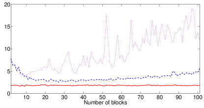
(a) $0.8$-quantile of the distance between the true localization and the estimated position. The localization error is given with the nonaveraged estimate (dotted line), the averaged estimate (dashed line) and the optimal estimate (bold line).

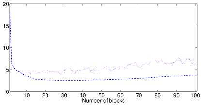
(b) Mean $\mathrm{L}_{1}$ error on the map estimate with the initial estimate (dotted line) and the averaged estimate (dashed line).

Figure 2: Errors on the map estimation and localization processes with the original algorithm.

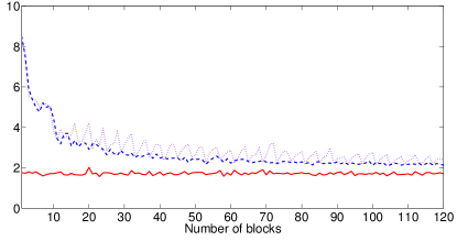
(a) $0.8$-quantile of the distance between the true localization and the estimated position with the stabilization process. The localization error is given with the nonaveraged estimate (dotted line), the averaged estimate (dashed line) and the optimal estimate (bold line).

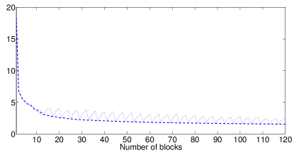
(b) Mean $\mathrm{L}_{1}$ error on the map estimate with the initial estimate (dotted line) and the averaged estimate (dashed line) with the stabilization process.

Figure 3: Errors on the map estimation and localization procedure with the stabilized algorithm.

Figures 4 and 5 illustrate the performance of the algorithm for the localization and for the estimation of the maps over $50$ independent Monte Carlo runs. In Figure 4, the optimal localization error (i.e. when the maps are known) is also displayed. The convergence of the localization error to the optimal error is almost reached after $100$ blocks (about $100000$ observations). Similarly, the error for the estimation of the maps given by the averaged algorithm goes on decreasing after $100$ blocks (the decrease is slower after $75$ blocks).

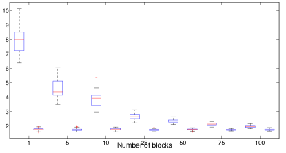
Figure 4: Boxplots of the localization error given by the stabilized algorithm with the averaged estimate (left) and the optimal estimate (right) as a function of the number of blocks.

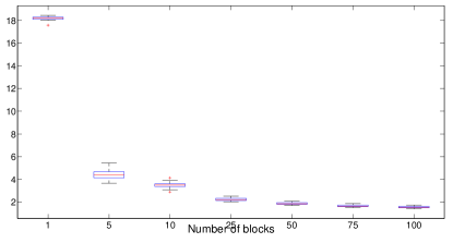
Figure 5: Boxplots of the mean $\mathrm{L}_{1}$ error on the map estimate with the stabilized algorithm and the averaged estimate as a function of the number of blocks.

V-B True data

In this section, the behaviour of our SLAM algorithm is illustrated in a real situation. 10 access points are set up in an office environment (Figure  6 represents a map of this environment as well as the position of the access points). The map is discretized using a grid $\mathcal{C}\subset[0,30]\times[0,30]$.

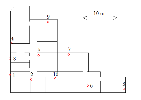
Figure 6: Map of the indoor environment used for the test with the position the access points (red circles) and their associated identification numbers.

The variance $\sigma^{\star,2}$ is assumed to be known and its value ($\sigma^{\star,2}=25dBm^{2}$) is calibrated using a measurement campaign at a fixed position. Around $T=20000$ measures of the RSSI have been made on the map using a WiFi device. Algorithm 2 produces position estimates but we do not have a direct access to the real position and thus cannot observe the localization error. To overcome this difficulty, a test data sample is built by producing measures along 12 paths in the environment such that, for each measure, the associated position is registered. The test data sample is made of $T_{\text{test}}=1100$ measures: $\{X_{t}^{\text{test}},Y_{t}^{\text{test}}\}_{t=1}^{T_{\text{test}}}$. The test data sample is used to compare the localization accuracy provided by different values of the parameter $F$. Note a major difference between the model given in Section II and the real data situation. For any measure $Y$ sent by the device, only several APs are represented in $Y$. Therefore, the maps $\widetilde{F}_{j}$, $j\in\{1,\ldots,B\}$ are not estimated simultaneously as, for any time step $t$, two APs might appear a different number of times in $Y_{1:t}$. We thus slightly modify Algorithm 2 by introducing specific blocks and measure counters relatively to each AP. Each time the value of $\widetilde{F}_{j}$ for any $j\in\{1,\ldots,B\}$ is updated using a block of the $20000$ measures, we submit the new estimator $\widetilde{F}$ to the test data sample: Algorithm 2 is run on the test data sample $\{Y_{t}^{\text{test}}\}_{t=1}^{T_{\text{test}}}$. Only the averaged particle system is computed and no parameter update is performed. We can then compute the localization error relatively to the test data sample as the 0.8-quantile of the error between $\{X_{t}^{\text{test}}\}_{t=1}^{T_{\text{test}}}$ and the averaged position estimate. Figure 7 displays the results of this experiment by representing the 0.8-quantile of the error as a function of the number of updates. The numbers on the graph in Figure 7 indicate which AP were updated for each update. The initial map estimates are given, for any $j\in\{1,\ldots,10\}$ by $c^{0}_{1,j}=-26$ and $c^{0}_{2,j}=-17.5$ and $\delta_{0}=0$.

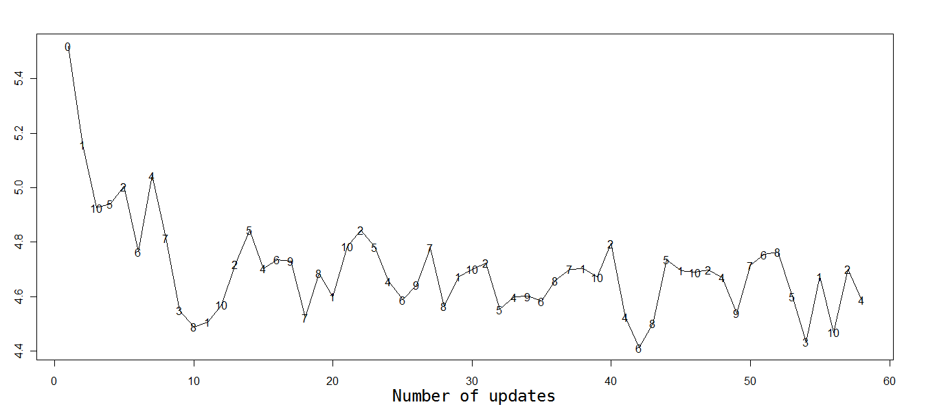
Figure 7: 0.8-quantile of the distance (in meter) between the true localization and the averaged estimate obtained with the stabilized algorithm. The localization error is computed on the test data sample each time one of the estimated map is updated.

Despite the relatively small test sample size, Figure 7 shows that the localization error seems to adopt the same behaviour as the localization error for the simulated data. The parameter $F_{j}$ was updated a maximum of $7$ times (for AP $j=10$ for instance) and a minimum of $2$ times (for AP $j=3$).

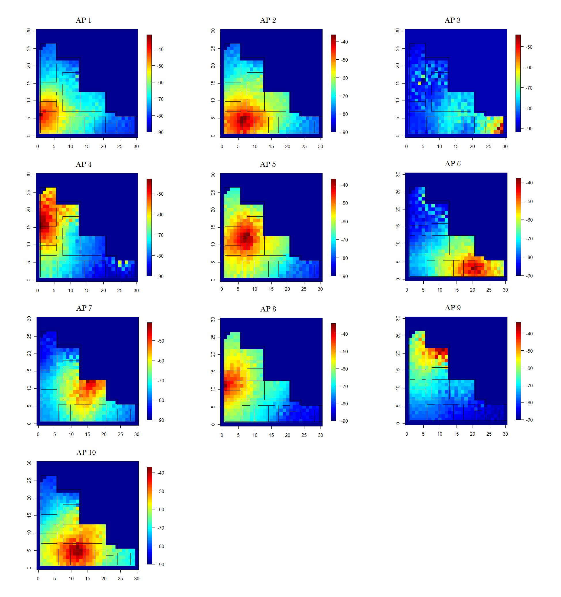
Figure 8: Graphical representation of the final propagation maps estimations: $\{\widetilde{F}_{j}\}_{j=1}^{10}$ (in $dBm$).

Figure 8 represents the final estimate of the propagation maps $\widehat{F}_{j}$, $j\in\{1,\ldots,10\}$. For some map estimates (see for instance the access points $1$, $4$ and $7$), the signal strength drops when passing walls while the walls are responsible for a part of the indoor waves propagation disturbances.

VI Conclusion

In this paper we propose a stabilized version of the BOEM algorithm to estimate the signal propagation maps needed in any WiFi based localization system. The main difference with the existing solutions is that these propagation maps are estimated using the data sent by the mobile device originally used for localization purposes. On the contrary, the existing WiFi based localization systems establish these propagation maps either in a deterministic way or by running a previous hand made survey. In case of environmental modifications, the propagation maps are thereby changed. Our technique can easily be adapted to these changes by regularly reinitializing the sufficient statistics while hand made survey based systems can not take into account these modifications without renewing the survey. However, further tests are needed to evaluate the accuracy provided by our method and to compare it with other methods. Many elements should be analyzed such as the number and the position of the access points, the size of the environment or the materials constituting the obstacles in the environment.

References

- [1] E. Gaura, L. Girod, J. Brusey, M. Allen, and G. Challen, Wireless Sensor Networks: Deployments and Design Frameworks. Springer, 2010.
- [2] G. Barrenetxea, F. Ingelrest, G. Schaefer, and M. Vetterli, “Wireless Sensor Networks for Environmental Monitoring: The SensorScope Experience,” in The 20th IEEE International Zurich Seminar on Communications (IZS 2008), 2008, invited paper.
- [3] S.-Y. Lau, T.-H. Lin, T.-Y. Huang, I.-H. Ng, and P. Huang, “A measurement study of zigbee-based indoor localization systems under rf interference,” in Proceedings of the 4th ACM international workshop on Experimental evaluation and characterization, ser. WINTECH ’09. New York, NY, USA: ACM, 2009, pp. 35–42. [Online]. Available: http://doi.acm.org/10.1145/1614293.1614300
- [4] P. Bahl and V. N. Padmanabhan, “Radar: an in-building rf-based user location and tracking system,” INFOCOM 2000. Nineteenth Annual Joint Conference of the IEEE Computer and Communications Societies. Proceedings. IEEE, vol. 2, pp. 775–784 vol.2, 2000. [Online]. Available: http://dx.doi.org/10.1109/INFCOM.2000.832252
- [5] Y.-C. Chen, J.-R. Chiang, H.-h. Chu, P. Huang, and A. W. Tsui, “Sensor-assisted wi-fi indoor location system for adapting to environmental dynamics,” in Proceedings of the 8th ACM international symposium on Modeling, analysis and simulation of wireless and mobile systems, ser. MSWiM ’05. New York, NY, USA: ACM, 2005, pp. 118–125. [Online]. Available: http://doi.acm.org/10.1145/1089444.1089466
- [6] J. M. Gorce, K. Jaffres-Runser, and G. D. L. Roche, “Deterministic approach for fast simulations of indoor radio wave propagation,” pp. 938–948, 2007. [Online]. Available: http://ieeexplore.ieee.org/lpdocs/epic03/wrapper.htm?arnumber=4120260
- [7] F. Evennou and F. Marx, “Advanced integration of wifi and inertial navigation systems for indoor mobile positioning,” EURASIP J. Appl. Signal Process., vol. 2006, pp. 164–164, Jan. 2006. [Online]. Available: http://dx.doi.org/10.1155/ASP/2006/86706
- [8] B. Ferris, D. Hähnel, and D. Fox, “Gaussian processes for signal strength-based location estimation,” in Robotics: Science and Systems’06, 2006.
- [9] H. T. Friis, “A note on a simple transmission formula,” Proceedings of the IRE, vol. 34, no. 5, pp. 254–256, Sep. 2006. [Online]. Available: http://ieeexplore.ieee.org/xpls/abs_all.jsp?arnumber=1697062
- [10] A. P. Dempster, N. M. Laird, and D. B. Rubin, “Maximum likelihood from incomplete data via the EM algorithm,” J. Roy. Statist. Soc. B, vol. 39, no. 1, pp. 1–38 (with discussion), 1977.
- [11] O. Cappé and E. Moulines, “Online Expectation Maximization algorithm for latent data models,” J. Roy. Statist. Soc. B, vol. 71, no. 3, pp. 593–613, 2009.
- [12] G. Mongillo and S. Denève, “Online learning with hidden Markov models,” Neural Computation, vol. 20, no. 7, pp. 1706–1716, 2008.
- [13] O. Cappé, “Online EM algorithm for Hidden Markov Models,” To appear in J. Comput. Graph. Statist., 2011.
- [14] O. Cappé, “Online sequential Monte Carlo EM algorithm,” in IEEE Workshop on Statistical Signal Processing (SSP), 2009.
- [15] M. Del Moral, A. Doucet, and S. Singh, “Forward smoothing using sequential Monte Carlo,” Dec 2010, preprint.
- [16] S. Le Corff, G. Fort, and E. Moulines, “Online EM algorithm to solve the SLAM problem,” in IEEE Workshop on Statistical Signal Processing (SSP), 2011.
- [17] S. Le Corff and G. Fort, “Online Expectation Maximization based algorithms for inference in Hidden Markov Models,” arXiv, Tech. Rep., 2011.
- [18] O. Cappé, E. Moulines, and T. Rydén, Inference in Hidden Markov Models. Springer, 2005.
- [19] O. Cappé, “Recursive computation of smoothed functionals of hidden Markovian processes using a particle approximation,” Monte Carlo Methods Appl., vol. 7, no. 1–2, pp. 81–92, 2001.
- [20] P. Del Moral, Feynman-Kac Formulae. Genealogical and Interacting Particle Systems with Applications. Springer, 2004.
- [21] A. Doucet and A. Johansen, “A tutorial on particle filtering and smoothing: fifteen years later,” Oxford handbook of nonlinear filtering, 2009.