How fast do Jupiters grow? Signatures of the snowline and growth rate in the distribution of gas giant planets

Abstract

We present here observational evidence that the snowline plays a significant role in the formation and evolution of gas giant planets. When considering the population of observed exoplanets, we find a boundary in mass-semimajor axis space that suggests planets are preferentially found beyond the snowline prior to undergoing gap-opening inward migration and associated gas accretion. This is consistent with theoretical models suggesting that sudden changes in opacity – as would occur at the snowline – can influence core migration. Furthermore, population synthesis modelling suggests that this boundary implies that gas giant planets accrete $\sim 70$ % of the inward flowing gas, allowing $\sim 30$ % through to the inner disc. This is qualitatively consistent with observations of transition discs suggesting the presence of inner holes, despite there being ongoing gas accretion.

1 Introduction

Since the discovery, in 1995, of the first extrasolar planet around a main-sequence star (Mayor & Queloz, 1995), a further 759 such planets have been detected. Many of these planets have masses similar to that of Jupiter and hence are generally regarded as gas giants. The standard model for the formation of these planets is the core accretion model (Pollack et al., 1996). In this model, micron-sized dust grains grow to form kilometre-sized planetesimals that then coagulate to form planetary mass bodies that, if sufficiently massive, may gravitationally attract a gaseous envelope if gas is still present in the disc.

Population synthesis models (Ida & Lin, 2004; Alibert et al., 2005) have generally been successful in reproducing the properties of the observed exoplanet population. However, while these models have illustrated how the overall process leads to a population consistent with that observed, they have not specifically quantified any individual parts of the process.

It has, however, recently been noted (Wright et al., 2009) that the distribution in semimajor axis of the observed exoplanets shows a peak at $\sim 1$ AU. It has been suggested that this peak may be a consequence of disc dispersal through photoevaporation (Alexander & Pascucci, 2012). Some population synthesis models (Mordasini et al., 2012) have also managed to reproduce this peak in the semimajor axis distribution and suggest that it is an imprint of the snowline. The ices that collect on small dust grains sublimate inside the snowline, where the temperature in the disc exceeds 170 K. The snowline radius is 2.7 AU for a solar-mass star (Hayashi, 1981) and scales with $M^{2}$.

During the gas giant planet formation process, the rocky/icy core is expected to go through a phase of rapid inward migration, known as type I migration (Ward, 1997). Quite how these cores survive to form gas giant planets is still uncertain. This migration may, however, be strongly affected by regions with a sudden change in opacity, as would occur at the snowline (Menou & Goodman, 2004). To investigate this we consider the distribution of planets in semi-major axis space. In the left-hand panel of Figure 1 we plot planet mass against semimajor axis, while in the right-hand panel we plot planet mass against semimajor axis with the semimajor axis normalised with respect to the predicted snowline of the host star. We consider 463 exoplanets that were first detected by radial velocity measurements. In the left-hand panel there appears to be an excess of planets beyond 1 AU that has been highlighted by Wright et al. (2009) and others (Mordasini et al., 2012; Alexander & Pascucci, 2012). In the right-hand panel, however, there appears to be, for planet masses below a few Jupiter masses, quite a well-defined diagonal boundary across which there is a step increase in the density of planets.

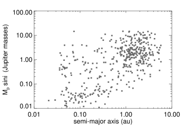
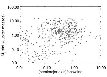
Figure 1: The left-hand panel shows planet mass against semimajor axis and illustrates an excess of planets beyond 1 AU (Wright et al., 2009). The right-hand panels shows planet mass against semimajor axis with the semimajor axis normalised with respect to the snowline of each exoplanets host star. In the right-hand panel, there appears to be quite a well-defined diagonal boundary, across which there is a step increase in the density of planets.

To characterise the diagonal boundary seen in the right-hand panel of Figure 1, we assume that it has the form $M\sin i/M_{\rm Jup}=\delta\left(a/a_{\rm snow}\right)^{\eta}$. We consider a box with $0.2\leq M/M_{\rm Jup}<7$ and $0.07\leq a/a_{\rm snow}<1$ and determine the values of $\delta$ and $\eta$ that produce the biggest density contrast. The solid line shows the boundary that produces the largest density contrast while the dashed and dotted lines shows two other solutions that lie on the extremes of the bootstrapped 49% confidence contour in $\delta-\eta$ space, discussed in more detail in Section A.

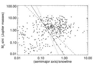
Figure 2: Planet mass against semimajor axis with the semimajor axis normalised with respect to the snowline of each exoplanets host star. There appears to be a diagonal boundary, in mass-semimajor axis space, across which there is a step increase in the density of planets. The solid line shows the boundary that produces the the largest density contrast while the dashed and dotted lines shows two other solutions that lie on the extremes of the bootstrapped 49% confidence contour in $\delta-\eta$ space.

If a planet is sufficiently massive, it can open a gap and migrate inwards via what is known as type II migration (Goldreich & Tremaine, 1980; Lin & Papaloizou, 1986). It can also continue growing by accreting some of the gas flowing though the gap (Lubow, Seibert & Artymowicz, 1999). During this phase, planet growth typically follows a diagonal line in $\log M$ - $\log a$ space (Mordasini et al., 2012). We, therefore, assume that the diagonal boundary in the right-hand panel of Figure 1, and characterised in Figure 2, is a consequence of this migration and gas accretion. The diagonal lines in Figure 2 have the form $M\sin i/M_{\rm Jup}=\delta\left(a/a_{\rm snow}\right)^{\eta}$ and so if $a_{o}=a_{\rm snow}$, $M_{o}=\delta$ M_Jup, which we interpret as suggesting that a planet forming at the snowline reaches a mass of $\delta$ M_Jup before starting to migrate inwards via type II migration and growing via associated gas accretion. For the best fit line (solid line), this corresponds to $M_{o}=0.01$ M_Jup, while for the dashed line it is $M_{o}=0.078$ M_Jup. These are both consistent with the mass at which we would expect type II migration to start operating (D’Angelo, Henning & Kley, 2003). The dotted line gives $M_{o}<0.01$ M_Jup which may be unphysically small. We can, however, then use this to predict where each planet was prior to the start of this process. If this process typically starts when the planets reach a mass of $M_{o}$, then from its current mass, $M_{p}$, and semimajor axis, $a$, its initial semimajor axis would be $a_{o}=a(M_{o}/M_{p})^{1/\eta}$. We thus determine the initial distribution of these planets, as shown in Figure 3, where the initial semimajor axis is normalised to the snowline and the line styles correspond to those in Figure 2. Figure 3 shows a definite jump at the snowline, with the largest density contrast occuring, as expected, for our best fit line.

The above suggests that prior to the final stages of planet formation (inward type II migration and final stage gas accretion), planets are preferentially found beyond the snowline of their host star. In this paper we, therefore, combine a realistic model of the evolution of protostellar discs with models of the growth and migration of gas giant planets to establish if this intepretation of the diagonal feature in Figure 2 is consistent with theoretical models of planet migration and growth.

Figure 3: Distribution of the initial semimajor axis, $a_{o}$, of the exoplanet population with $a_{o}$ normalised with respect to the expected snowline of the host star. In this case $a_{o}$ is determined by assuming that growth follows the diagonal line in Figure 2 and hence that $a_{o}=a(M_{o}/M_{p})^{-1/\eta}$ with $M_{o}=\beta$ M_Jup. The line styles correspond to those in Figure 2 and the largest density contrast occurs, as expected, for the best fit line in Figure 2.

2 Basic Model

2.1 Disc model

We assume that the disc is axisymmetric and use the standard one-dimensional equations (Lynden-Bell & Pringle, 1974; Pringle, 1981) to evolve the surface density, $\Sigma(r,t)$. The surface density evolution is largely determined by the kinematic viscosity, $\nu$, and by mass loss through a disc wind. We assume that the viscosity has the form of an $\alpha$ viscosity (Shakura & Sunyaev, 1973) so that $\nu=\alpha c_{s}H$, where $c_{s}$ is the disc sound speed, $H$ is the disc scaleheight, and $\alpha<<1$ is a parameter that determines the efficiency of angular momentum transport. It has recently been suggested (Owen et al., 2010) that x-rays are the dominant driver of photoevaporation, and so here we implement the x-ray photoionization model described in detail in Owen, Ercolano & Clarke (2011).

We ran 100 disc models and selected the central star mass randomly between $M_{\star}=0.8$ M_⊙ and $M_{\star}=1.2$ M_⊙. We don’t explicitly include the planets in these disc models, but instead use the range of disc models to later evolve planets with a large range of different initial conditions. We assume the disc extends from $r=0.1$ AU to $r=50$ AU with an initial surface density profile of $\Sigma\propto r^{-1}$. In each simulation the initial disc mass is $0.25M_{\star}$. The initial disc mass is therefore quite high and such discs are likely to be self-gravitating. Within $50$ AU (Rafikov, 2005), it is expected that such discs will achieve a state of quasi-steady thermal equilibrium with dissipation due to the gravitational instability balanced by radiative cooling (Gammie, 2001). It has been shown (Balbus & Papaloizou, 1999; Lodato & Rice, 2004) that the gravitational instability then acts to transport angular momentum in a manner analogous to viscous transport. As described in detail in Rice & Armitage (2009) (see also Clarke, 2009; Zhu, Hartmann & Gammie, 2009), this can then be used to determine the effective value of $\alpha$ and, hence, the kinematic viscosity, $\nu$.

If, however, the effective gravitational $\alpha$ is less than $0.005$, we assume that another transport mechanism, such as the magnetorotational instability (MRI) (Balbus & Hawley, 1991) will then dominate and we set $\alpha=0.005$. In addition, we also assume that irradiation from the central star sets a radially dependent minimum temperature in the disc (Hayashi, 1981). Although all of our disc models start with the same disc-to-star mass ratio, the variation in x-ray luminosity (from $5\times 10^{28}$ erg s^-1 to $10^{31}$ erg s^-1) produces a wide range of different disc lifetimes, largely consistent with that observed (Haisch, Lada & Lada, 2001). We therefore have a set of disc models that can self-consistently evolve the surface density from the early stages, when the gravitational instability is likely to dominate, through to the later stages when an alternative transport mechanism, such as MRI, will dominate and that also includes the late-stage dispersal due to photoevaporative mass-loss.

2.2 Core growth and migration

Planet formation is thought to occur through the initial growth of micron-sized dust grains to, ultimately, kilometre-size planetesimals. These planetesimals then continue to grow with, typically, the largest in any region dominating and undergoing what is known as oligarchic growth (Kokubo & Ida, 1998). If these oligarchs can grow sufficiently massive ($\sim 10$ M_⊕) then, if there is still gas present in the disc, they can gravitationally attract a gaseous envelope and can rapidly grow to become a gas giant planet.

Once a planetary mass body has formed, it can exchange angular momentum with the surrounding disc material and migrate radially (Goldreich & Tremaine, 1980). There a number of different migration scenarios. Low-mass planets ($M_{\rm pl}\sim 1$ M_⊕) generate a linear disc response and migrate inwards through what is known as type I migration (Ward, 1997). High-mass planets are thought to open a gap in the disc gas and migrate through type II migration (Lin & Papaloizou, 1986). A third type of migration, known as type III migration, may occur for intermediate mass planets (Masset & Papaloizou, 2003). In the type III regime, corotation torques generate very rapid migration which can be inward or outward (Masset & Papaloizou, 2003).

The migration rate for planets migrating in the type I regime increases with planet mass and analytic (Tanaka, Takeuchi & Ward, 2002) and numerical (Bate et al., 2003) estimates suggest that the timescale should be less than typical disc lifetimes. These planets should therefore migrate into the central star prior to becoming massive enough to enter the slower type II migration regime. Recent numerical simulations suggest that the type I migration rate can, however, be significantly reduced if the disc thermodynamics is treated more realistically (Paardekooper & Mellema, 2008; Paardekooper, Baruteau & Kley, 2011). Recent population synthesis models therefore typically assume that the analytic type I rate is reduced by at least a factor of about $30$ (Alibert et al., 2005). These models are now quite successful at reproducing the observed characteristics of the exoplanet population (Mordasini, Alibert & Benz, 2009; Alibert, Mordasini & Benz, 2011).

Furthermore, it has been suggested (Menou & Goodman, 2004) that type I migration can be strongly influenced by sudden changes in the disc opacity, such as may occur near the snowline. One of the goals of this paper is to investigate whether or not the possible infuence of the snowline on core migration is consistent with the observed distribution of extraolar planets. After type I and, potentially, type III migration have distributed the planetary cores throughout the disc, they then undergo continued growth through gas accretion and migrate via gap opening type II migration. We also want to compare the current distribution of exoplanets with a population synthesis–like model to determine if we can quantify type II migration and the growth that accompanies this migration process.

2.3 Type II migration and gas accretion

In our modelling we don’t explicitly model the growth of the cores and the initial runaway gas accretion phase (Ikoma, Nakazawa & Emori, 2000; Bryden et al., 2000) that occurs when the planetary core reaches the critical core mass (Ikoma, Nakazawa & Emori, 2000; Papaloizou & Terquem, 1999). The runaway gas accretion phase terminates when the planet reaches the gas isolation mass (Lissauer, 1987). We assume that the gas feeding zone is 2 Hill radii wide with the Hill radius of a planet with mass $M_{p}$ located at $a$ in the disc given by

$$r_{H}=a\left(\frac{M_{p}}{3M_{*}}\right)^{1/3}.$$ (1)

One can then show that the isolation mass is

$$M_{\rm iso}=\frac{(4\pi a^{2}\Sigma)^{3/2}}{(3M_{*})^{1/2}}.$$ (2)

As discussed in section 2.1 we have a series of disc models with central star masses between $M_{*}=0.8$ M_⊙ and $M_{*}=1.2$ M_⊙ and with a range of x-ray luminosities that results in a range of disc lifetimes that largely matches that observed (Haisch, Lada & Lada, 2001). The current exoplanet sample has more stars with mass $M_{*}>1$ M_⊙ than with masses $M_{*}<1$ M_⊙ and so we use the disc models with central star masses $>1$ M_⊙ twice as often as those with central star masses $<1$ M_⊙.

For each planet formation simulation, we assume that the planetary core forms and undergoes runaway gas accretion at a randomly chosen time between $t=1$ Myr and $t=4$ Myr. The disc model then gives us the mass of the central star and surface density and so Equation (2) can be used to determine the planet’s isolation mass. The disc model also gives the time dependence of the disc viscosity, $\nu$. If sufficiently massive, a planet will open a gap in the disc (Lin & Papaloizou, 1986). For a planet located at $a$, the width of the gap, $\Delta$, satisfies (Syer & Clarke, 1995)

$$\left(\frac{\Delta}{a}\right)^{3}=\frac{\Omega a^{2}}{\nu}q^{2},$$ (3)

where $q=M_{p}/M_{*}$. For a gap to open, the disc scaleheight, $H$, must be less than the gap width $\Delta$. A second criterion is that the gap width needs to be greater than the Roche radius, $R_{L}$, of the planet and hence

$$\Delta>R_{L}=q^{1/3}a\Rightarrow q>\frac{\nu}{\Omega a^{2}}.$$ (4)

If Equation (4) is satisfied and $H<\Delta$ then the planet is able to open a gap and migrate through type II migration.

Type II migration effectively has two regimes, the “disc dominated” regime (Armitage, 2007) and the “planet dominated” regime (Trilling et al., 1998). “Disc dominated” migration occurs when the local disc mass is large compared to the mass of the planet. In this case the planet is coupled to the viscous evolution of the disc and the migration rate is independent of the mass of the planet. The radial velocity of the planet is then

$$v_{pl}=-\frac{3\nu}{2a}.$$ (5)

If, however, $M_{p}>2\Sigma a^{2}$, the inertia of the planet reduces its radial velocity to

$$v_{pl}=-\frac{3\nu}{a}\frac{\Sigma a^{2}}{M_{p}}.$$ (6)

While migrating inwards, the planet is also able to accrete mass from the disc. For planets with mass of a few Jupiter masses, it has been suggested (Kley & Dirksen, 2006) that the planet could accrete at a rate comparable to gas accretion rate through the disc ($\dot{M_{*}}=3\pi\nu\Sigma$). We therefore assume that in the “planet dominated” migration regime the accretion rate onto the planet is

$$\dot{M}_{p}=\beta 3\pi\nu\Sigma,$$ (7)

with $\beta$ typically close to unity (Mordasini, Alibert & Benz (2009) assume $\beta=1$), and $\nu$ and $\Sigma$ coming from the self-consistent disc models. In the “disc dominated” regime we assume that this is reduced by a factor $1/B$ where $B=(2\pi\Sigma a^{2})/M_{p}$ is essentially the ratio of the local disc mass to the planet mass. The reduction is motivated by the mass accretion efficiency for planet growth determined by Veras & Armitage (2004) based on the results of two-dimensional numerical simulations (Lubow, Seibert & Artymowicz, 1999; D’Angelo, Henning & Kley, 2002).

We can combine Equations 6 and 7 to show that, in the “planet dominated” regime $\log{M_{p}/M_{o}}=\log{\left(a/a_{o}\right)^{-\beta\pi}}$. The dotted line in Figure 2 has a slope steeper than $-\pi$ which, given that $\beta\leq 1$, would appear to be unphysical if our simple interpretation is correct. We almost certainly need more data to determine, more accurately, the properties of this boundary.

2.4 Putting it all together

We randomly select one of our completed disc models and start modelling the evolution of the planet at the stage at which the planet semimajor axis has been set by type I (or type III) migration and the planet has just undergone runaway gas accretion. The initial planet mass is given by Equation (2) with $\Sigma$ taken from our chosen time-dependent disc model. Given the planet mass and semimajor axis, we use Equations (3) and (4) to determine if the planet opens a gap in the disc. If not, we assume that it grows slowly ($\dot{M}_{p}=0.1\dot{M}_{*}$ with $\dot{M}_{*}$ determined from our chosen disc model) and remains at its initial semimajor axis until it either does satisfy the gap opening criteria, or the gas disc has dispersed. If the gap opening criteria are satisfied then Equation (5) or (6) is used to determine the inward migration rate. The rate at which the planet grows is then given by Equation (7) with $\beta$ either a constant (in the “planet dominated” regime) or a constant reduced by $1/B$ (in the “disc dominated” regime). We stop either when the planet reaches $a=0.1$ AU (the inner edge of our disc models) or when the gas disc has dispersed. To synthesise a population of exoplanets, we repeat the above for different disc models and for different initial starting times and initial semimajor axes.

3 Results

In these simulations we assume that the sudden change in opacity at the snowline (Menou & Goodman, 2004) results in planetary cores being preferentially found beyond the snowline, rather than inside the snowline. We therefore assume, somewhat arbitrarily, that the exoplanet density is about 6 times lower inside the snowline than it is just outside the snowline. We also assume that type I migration results in a pile-up at the snowline and hence that the distribution beyond the snowline is uniform in $\log a$. The only other free parameter we have is $\beta$, the ratio of the gas accretion rate onto the planet to the gas accretion rate through the disc.

Figure 4 shows results for 3 different planet growth rates, $\beta$. The left-hand panel is for $\beta=0.5$, the middle panel is for $\beta=0.7$, and the right-hand panel is for $\beta=0.9$. The top row of figures shows planet mass against semimajor axis for $\sim 1000$ simulated planets and with the semimajor axis normalised with respect to the snowline of the planet’s host star. For each planet, we have also randomly selected an inclination angle such as to produce an isotropic distribution of orbit orientations. We also only show those that would have been detected with a $20$ year radial velocity campaign with a cadence of $1$ month and a rms velocity sensitivity of $1$ m s^-1. The diagonal lines are the same as that in Figure 2. Figure 4 already shows that for $\beta=0.5$ the density jump occurs inside the diagonal lines, while for $\beta=0.9$, it appears to be - largely - beyond the diagonal lines. The best match to that observed (Figure 2) appears to be the middle figure in the top panel in Figure 4 in which $\beta=0.7$.

As discussed in relation to Figure 3, we can use the diagonal lines to predict where each planet emerged prior to the start of type II migration and associated gas accretion. This is shown in the middle row of Figure 4. The middle figure of this row ($\beta=0.7$) is very similar to that seen in Figure 3 and suggests that, prior to type II migration, the planet population peaks at the snowline and that planets then grow in a manner consistent with the diagonal boundary in Figure 2. However, for $\beta=0.5$ and $\beta=0.9$, the peaks fall inside and beyond the snowline respectively.

The slope of the diagonal boundary is largely determined by the relationship between the rate at which the planet migrates inwards and the rate at which it grows. The bottom row of Figure 4 shows a sample of growth tracks for each $\beta$ value. This illustrates that the slope of the growth tracks in mass-semimajor axis space depends on the value of $\beta$ (the ratio of the accretion rate onto the planet to the gas accretion rate through the disc). The slope of the boundary in mass-semimajor axis space (top figures in Figure 4) appears not to precisely match the slope of the growth tracks, but is clearly influenced by the slope of these growth tracks. If $\beta>0.7$, the diagonal line would be steeper than that observed in Figure 1, while if $\beta<0.7$, the diagonal line would be shallower. The tracks also show that these planets are typically migrating in the “planet dominated” regime rather than in the “disc dominated” regime.

Figure 4: Series of figures for 3 different planet accretion rates. The planetary accretion is represented by $\beta$, the ratio of the accretion rate onto the planet to the gas accretion rate through the disc. The left-hand panel is for $\beta=0.5$, the middle panel is for $\beta=0.7$, and the right-hand panel is for $\beta=0.9$. The top row shows the final state distribution of planet mass and orbit semimajor axis, normalised with respect to the snowline, after the planet’s upward growth and inward migration are halted by photo-evaporation of the disc. The middle panel is the distribution of the initial semimajor axis ($a_{o}$ – determined in the same way as for Figure 3 and normalised with respect to the snowline of the host star) for the 3 different boundaries illustrated by the solid, dashed and dotted lines in the top set of figures. The bottom is a sample of $100$ planet growth tracks showing how the planets grow while migrating inwards through the disc.

4 Discussion and Conclusions

We use self-consistent disc simulations together with models of gas giant planet migration and growth to show that if the snowline influences core migration, as suggested by Menou & Goodman (2004), we can largely reproduce the observed planet mass against semimajor axis distribution. This in itself is interesting as it indicates that the snowline plays a crucial role in preventing planetary cores from migrating (via type I migration) into the host star. Furthermore, we use this to quantify the gas accretion rate onto the planet during the “planet dominated” type II migration phase. We find that it must accrete at a rate of about $70$ % that of the gas accretion rate through the disc. This is the first time that we have been able to quantify the rate at which a gas giant planet grows during the final stages of disc evolution.

Our results indicate that during type II migration a gas giant planet consumes $\sim 70$ % and allows $\sim 30$ % of the gas to flow inward. As a result, we expect a slightly lower gas density inside the planet’s orbit. It has also been suggested, however, that dust filtration at the gap edge (Rice et al., 2006) will prevent all but the smallest dust grains from reaching the inner disc, significantly enhancing the gas-to-dust ratio. This is consistent with observations of transition discs (Espaillat et al., 2010) which have near-IR deficits indicating a lack of warm dust in the inner disc, but still appear to be accreting at TTauri–like rates.

Appendix A Data analysis

To measure the slope of the observed linear feature in $\log{M/M_{J}}$-$\log{a/a_{\rm snow}}$ space, we aim to fit a straight line

$$\log(a/a_{\mathrm{snow}})=c+\alpha[\log(M\sin i/M_{\mathrm{J}})-\log 7],$$ (8)

to the data so that it maximizes the density ratio on either side of the line. This is related to the fitting parameters ($\delta$,$\eta$) that we use in the paper above through $\eta=1/\alpha$ and $\delta=10^{c-\alpha\log 7}$. To exclude other features of the simulated and observed planet distributions we select only planets with $0.2\leq M/M_{\mathrm{J}}<7$ and $0.07\leq a/a_{\mathrm{snow}}<1$, and measure the planet density on each side of this box, as divided by the line. In order to penalize solutions that maximized the density ratio by producing a small area on either side of the line, we actually maximized the quantity $\sqrt{N_{+}N_{-}}\rho_{+}/\rho_{-}$, which we call the fitting metric, where $\rho_{+/-}$ is the planet density to the right/left of the line, and $N_{+/-}$ is the number of planets to the right/left of the line. For the observed planets, to account for the varying detection efficiency as a function of the radial velocity semiamplitude $K$, we considered planets with $K<2.84$ m s^-1 to contribute a count of $(2.84$ m s${}^{-1}/K)$ to $\rho_{+/-}$ and $N_{+/-}$.

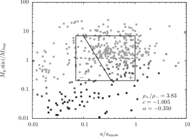
Figure 5: Plot of $M\sin i$ against $a/a_{\mathrm{snow}}$ for the observed planet distribution. The box shows the selection of planets that are used to fit a linear density feature. The diagonal line (equation 8) is the best fitting line that maximizes the density ratio on each side of the line. Other details are explained in the text.

Figure 5 shows the observed planet distribution with the best fitting line, which has parameters $c=-1.005$ and $\alpha=-0.350$. It is clear by eye that the number density of planets is significantly higher to the right of this line – the density contrast is $\rho_{+}/\rho_{-}=3.83$. In the plot, planets are shaded by their RV semiamplitude, such that the planets with the lightest grey are unweighted (i.e. $K>2.84$ m s^-1 and they count as $1$ planet) and black indicates $K=0$ m s^-1. The point with the smallest RV semiamplitude in the fitting box has $K=0.91$ m s^-1 and so counts as $3.1$ planets.

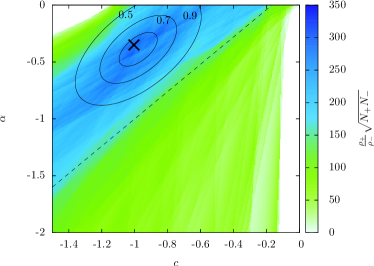
Figure 6: Map of the fitting metric plotted against the parameters $c$ (intercept) and $\alpha$ (slope) of the line fitted to the density feature seen in the observed planet distribution. The cross marks the best-fit solution for the observed distribution, and numbers denoting the $\beta$ value for simulated planet distributions are placed at the corresponding best-fit parameters. The black contours show estimated $68$- and $95$-percent confidence intervals for the observed planet solution based on a form of bootstrap resampling, while the dashed line was used to discard outlier solutions from this bootstrap analysis.

Figure 6 shows the fitting metric $\sqrt{N_{+}N_{-}}\rho_{+}/\rho_{-}$ mapped against the two parameters of the line. However, it is not possible to estimate the parameter uncertainties from the fitting metric as it does not obey $\chi^{2}$ statistics. Instead, we can estimate the uncertainties by a form of bootstrapping. To estimate the uncertainties by bootstrapping, we produced fake planet distributions by Poisson sampling from the observed planet number density (including $K$ weighting) in four uneven quadrants of the fitting box. The interior boundaries of the quadrants were defined by the best fitting line and the horizontal dashed line in Figure 5 at the center of the selected mass range. The density in each quadrant was assumed to be uniform in $\log(a/a_{\mathrm{snow}})$ and $\log(M\sin i/M_{\mathrm{J}})$. Each fake distribution is then fitted in the same way as the observed distribution, yielding an estimate of the parameters $c$ and $\alpha$ in each case. A small number ($6$ percent) of the bootstrap samplings produce solutions far from the best fit parameters for the observed planets, and are distributed roughly uniformly over the lower right half of the $c$-$\alpha$ parameter space (in the lower, green region in Figure 6), while the majority of samplings lie near the observed planet solution, with a distribution that roughly follows the degeneracy suggested by the map of the fitting metric. The outlier points significantly skew estimates of the error ellipse so we discard samples that fall below the dashed line in Figure 6. The contours in the figure show the $49$-, $70$- and $85$-percent confidence intervals for a Gaussian with mean and covariances matching the remaining bootstrap sample, while the cross marks the position of the solution for the observed planet distribution and numbers indicate the solutions for the simulated data sets with different values of $\beta$. It is clear that of the simulated planet distributions, the properties of the linear density feature in the simulation with $\beta=0.7$ best match those of the feature in the observed distribution.

References

- Alexander & Pascucci (2012) Alexander R.D., Pascucci I., 2012, MNRAS, in press
- Alibert, Mordasini & Benz (2011) Alibert Y., Mordasini C., Benz W., 2011, A&A, 526, 63
- Alibert et al. (2005) Alibert Y., Mordasini C., Benz W., Winisdoerffer C., 2005, A&A, 434, 343
- Armitage (2007) Armitage P.J., 2007, ApJ, 665, 1381
- Balbus & Hawley (1991) Balbus S.A., Hawley J.F., 1991, ApJ, 376, 214
- Balbus & Papaloizou (1999) Balbus S.A., Papaloizou J.C.B., 1999, ApJ, 521, 650
- Bate et al. (2003) Bate, M.R., Lubow, S.H., Ogilvie, G.I., & Miller, K.A. 2003, MNRAS, 341, 213
- Bryden et al. (2000) Bryden G., Różycka M., Lin D.N.C., Bodenheimer P., 2000, ApJ, 540, 1091
- Clarke (2009) Clarke C.J., 2009, MNRAS, 396, 1066
- D’Angelo, Henning & Kley (2002) D’Angelo G., Henning T., Kley W., 2002, A&A, 385, 647
- D’Angelo, Henning & Kley (2003) D’Angelo G., Henning T., Kley W., 2003, ApJ, 586, 540
- Espaillat et al. (2010) Espaillat C., et al., 2010, ApJ, 717, 441
- Gammie (2001) Gammie C.F., 2001, ApJ, 553, 174
- Goldreich & Tremaine (1980) Goldreich P., Tremaine S., 1980, ApJ, 241, 425
- Greaves & Rice (2010) Greaves J.S., Rice W.K.M., 2010, MNRAS, 407, 1981
- Haisch, Lada & Lada (2001) Haisch K.E., Lada E.A., Lada C.J., 2001, AJ, 121, 2065
- Hayashi (1981) Hayashi C., 1981, Prog. Thoer. Phys. Suppl., 70, 35
- Ida & Lin (2004) Ida S., Lin D.N.C., 2004, ApJ, 616, 567
- Ikoma, Nakazawa & Emori (2000) Ikoma M., Nakazawa K., Emori H., 2000, ApJ, 537, 1013
- Kley & Dirksen (2006) Kley W., Dirksen G., 2006, A&A, 447, 369
- Kokubo & Ida (1998) Kokubo E., Ida S., 1998, Icarus, 131, 171
- Lin & Papaloizou (1986) Lin D.N.C., Papaloizou J.C.B., 1986, MNRAS, 309, 846
- Lissauer (1987) Lissauer J.J., 1987, Icarus, 69, 249
- Lodato & Rice (2004) Lodato G., Rice W.K.M., 2004, MNRAS, 351, 630
- Lubow, Seibert & Artymowicz (1999) Lubow S.H., Seibert M., Artymowicz P., 1999, ApJ, 526, 1001
- Lynden-Bell & Pringle (1974) Lynden-Bell D., Pringle J.E., 1974, MNRAS, 168, 603
- Masset & Papaloizou (2003) Masset F.S., Papaloizou J.C.B., 2003, ApJ, 588, 494
- Mayor & Queloz (1995) Mayor M., Queloz D., 1995, Nature, 378, 355
- Menou & Goodman (2004) Menou K., Goodman J., 2004, ApJ, 606, 520
- Mordasini et al. (2012) Mordasini C., Alibert Y., Benz W., Klahr H., Henning T., 2012, A&A, in press.
- Mordasini, Alibert & Benz (2009) Mordasini C., Alibert Y., Benz W., 2009, A&A, 501, 1139
- Owen et al. (2010) Owen J.E., Ercolano B., Clarke C.J., Alexander R.D., 2010, MNRAS, 401, 1415
- Owen, Ercolano & Clarke (2011) Owen J.E., Ercolano B., Clarke C.J., 2011, MNRAS, 412, 13
- Paardekooper & Mellema (2008) Paardekooper S.-J., Mellema G., 2008, A&A, 478, 245
- Paardekooper, Baruteau & Kley (2011) Paardekooper S.-J., Baruteau C., Kley W., 2011, 410, 293
- Papaloizou & Terquem (1999) Papaloizou J.C.B., Terquem C., 1999, ApJ, 521, 823
- Pollack et al. (1996) Pollack J.B., Hubickyj O., Bodenheimer P., Lissauer J.J., Podolak M., Greenzweig Y., 1996, Icarus, 124, 62
- Pringle (1981) Pringle J.E., 1981, ARA&A, 19, 137
- Rafikov (2005) Rafikov R.R., 2005, ApJ, 621, L69
- Rice & Armitage (2009) Rice W.K.M., Armitage P.J., 2009, MNRAS, 396, 2228
- Rice et al. (2006) Rice W.K.M., Armitage P.J., Wood K., Lodato G., 2006, MNRAS, 373, 1619
- Shakura & Sunyaev (1973) Shakura, N.I., & Sunyaev, R.A. 1973, A&A, 24, 337
- Syer & Clarke (1995) Syer D., Clarke C., 1995, MNRAS, 277, 758
- Tanaka, Takeuchi & Ward (2002) Tanaka H., Takeuchi T., Ward W.R., 2002, ApJ, 565, 1257
- Trilling et al. (1998) Trilling D.E., Benz W., Guillot T., Lunine J.I., Hubbard W.B., Burrows A., 1998, ApJ, 500, 428
- Veras & Armitage (2004) Veras D., Armitage P.J., 2004, MNRAS, 347, 613
- Ward (1997) Ward, W.R. 1997, Icarus, 126, 261
- Wright et al. (2009) Wright J.T., Upadhyay S., Marcy G.W., Fischer D.A., Ford E.B., Johnson J.A., 2009, ApJ, 693, 1084
- Zhu, Hartmann & Gammie (2009) Zhu Z., Hartmann L., Gammie C.F., 2009, ApJ, 694, 1045