Efficient Estimation of Approximate Factor Models via Regularized Maximum Likelihood
Abstract
We study the estimation of a high dimensional approximate factor model in the presence of both cross sectional dependence and heteroskedasticity. The classical method of principal components analysis (PCA) does not efficiently estimate the factor loadings or common factors because it essentially treats the idiosyncratic error to be homoskedastic and cross sectionally uncorrelated. For efficient estimation it is essential to estimate a large error covariance matrix. We assume the model to be conditionally sparse, and propose two approaches to estimating the common factors and factor loadings; both are based on maximizing a Gaussian quasi-likelihood and involve regularizing a large covariance sparse matrix. In the first approach the factor loadings and the error covariance are estimated separately while in the second approach they are estimated jointly. Extensive asymptotic analysis has been carried out. In particular, we develop the inferential theory for the two-step estimation. Because the proposed approaches take into account the large error covariance matrix, they produce more efficient estimators than the classical PCA methods or methods based on a strict factor model.
Keywords: High dimensionality, unknown factors, principal components, sparse matrix, conditional sparse, thresholding, cross-sectional correlation, penalized maximum likelihood, adaptive lasso, heteroskedasticity
1 Introduction
In many applications of economics, finance, and other scientific fields, researchers often face a large panel data set in which there are multiple observations for each individual; here individuals can be families, firms, countries, etc. Modern applications usually involve data-rich environments in which both the number of observations for each individual and the number of individuals are large. One useful method for summarizing information in a large dataset is the factor model:
| (1.1) |
where is an individual effect, is an vector of factor loadings and is an vector of common factors; denotes the idiosyncratic component of the model. Note that is the only observable random variable in this model. If we write , , and , then model (1.1) can be equivalently written as
Because is the only observable in the model, both factors and loadings are treated as parameters to estimate. As was shown by Chamberlain and Rothschild (1983), in many applications of factor analysis, it is desirable to allow dependence among the error terms not only serially but also cross-sectionally. This gives rise to the approximate factor model, in which the covariance matrix is not diagonal. In addition, the diagonal entries may vary in a large range. As a result, efficiently estimating the factor model under both large and large is difficult because to take into account both cross-sectional heteroskedasticity and dependence of , it is essential to estimate the large covariance . The latter has been known as a challenging problem when is larger than .
In this paper, we assume the model to be conditionally sparse, in the sense that is a sparse matrix with bounded eigenvalues. This assumption effectively reduces the number of parameters to be estimated in the model, and allows a consistent estimation of . The latter is needed to efficiently estimate the factor loadings. In addition, it enables the model to identify the common components asymptotically as . We propose two alternative methods, both are likelihood-based. The first one is a two-step procedure. In step one, we apply the principal orthogonal complement thresholding (POET) estimator of Fan et al. (2012) to estimate using the adaptive thresholding as in Cai and Liu (2011); in step two, we estimate the factor loadings by maximizing a Gaussian-quasi likelihood function, which depends on the covariance estimator in the first step. These two steps can be carried out iteratively. We also propose an alternative method for jointly estimating the factor loadings and the error covariance matrix by maximizing a weighted penalized likelihood function. The likelihood penalizes the estimation of the off-diagonal entries of the error covariance and automatically produces a sparse covariance estimator. We present asymptotic analysis for both methods. In particular, we derive the uniform rate of convergence and limiting distribution of the estimators for the two-step procedure. The analysis of the joint-estimation is more difficult as it involves penalizing a large covariance with diverging eigenvalues. We establish the consistency for this method.
Moreover, we achieve the “sparsistency” for the estimated error covariance matrix in factor analysis (see Section 3 for detailed explanations). The estimated covariance is consistent for both approaches under the normalized Frobenius norm even when is much larger than . This is important in the applications of approximate factor models.
There has been a large literature on estimating the approximate factor model. Stock and Watson (1998, 2002) and Bai (2003) considered the principal components analysis (PCA), and they developed large-sample inferential theory. However, the PCA essentially treats to have the same variance across , hence is inefficient when cross-sectional heteroskedasticity is present. Choi (2012) proposed a generalized PCA that requires to invert the error sample covariance matrix. More recently, Bai and Li (2012) estimated the factor loadings by maximizing the Gaussian-quasi likelihood, which addresses the heteroskedasticity under large , but they consider the strict factor model in which are uncorrelated. Additional literature on factor analysis includes, e.g., Bai and Ng (2002), Wang (2009), Dias, Pinherio and Rua (2008), Breitung and Tenhofen (2011), Han (2012), etc; most of these studies are based on the PCA method. In contrast, our methods are maximum-likelihood-based. Maximum likelihood methods have been one of the fundamental tools for statistical estimation and inference.
Our approach is closely related to the large covariance estimation literature, which has been rapidly growing in recent years. There are in general two ways to estimate a sparse covariance in the literature: thresholding and penalized maximum likelihood. For our two-step procedure, we apply the POET estimator recently proposed by Fan et al. (2012), corresponding to the thresholding approach of Bickel and Levina (2008a), Rothman et al. (2009) and Cai and Liu (2011). For the joint estimation procedure, we use the penalized likelihood, corresponding to that of Lam and Fan (2009), Bien and Tibshirani (2011), etc. In either way, we need to show that the impact of estimating the large covariances is asymptotically negligible for an efficient estimation, which is not easy in our context since the likelihood function is highly nonlinear, and contains a few eigenvalues that grow very fast. It was recently shown by Fan et al. (2012) that estimating a covariance matrix with fast diverging eigenvalues is a challenging problem. Other works on large covariance estimation include Cai and Zhou (2012), Fan et al. (2008), Jung and Marron (2009), Witten, Tibshirani and Hastie (2009), Deng and Tsui (2010), Yuan (2010), Ledoit and Wolf (2012), El Karoui (2008), Pati et al. (2012), Rohde and Tsybakov (2011), Zhou et al. (2011), Ravikumar et al. (2011) etc.
This paper focuses on high-dimensional static factor models although the factors and errors can be serially correlated. The model considered is different from the generalized dynamic factor models as in Forni, Hallin, Lippi and Reichlin (2000), Forni and Lippi (2001), Hallin and Liška (2007), and other references therein. Both static and dynamic factor models are receiving increasing attention in applications of many fields.
The paper is organized as follows. Section 2 introduces the conditional sparsity assumption and the likelihood function. Section 3 proposes the two-step estimation procedure. In particular, we present asymptotic inferential theory of the estimators. Both uniform rate of convergence and limiting distributions are derived. Section 4 gives the joint estimation as an alternative procedure, where we demonstrate the estimation consistency. Section 5 illustrates some numerical examples which compare the proposed methods with the existing ones in the literature. Finally, Section 6 concludes with further discussions. All proofs are given in the appendix.
Notation
Let and denote the maximum and minimum eigenvalues of a matrix respectively. Also Let , and denote the , spectral and Frobenius norms of , respectively. They are defined as , , . Note that is also the Euclidean norm when is a vector. For two sequences and , we write , and equivalently , if as
2 Approximate Factor Models
2.1 The model
The approximate factor model (1.1) implies the following covariance decomposition:
| (2.1) |
assuming to be uncorrelated with , where and denote the covariance matrices of and ; denotes the covariance of , all assumed to be time-invariant. The approximate factor model typically requires the idiosyncratic covariance have bounded eigenvalues and have eigenvalues diverging at rate . One of the key concepts of approximate factor models is that it allows to be non-diagonal.
Stock and Watson (1998) and Bai (2003) derived the rates of convergence as well as the inferential theory of the method of principal component analysis (PCA) for estimating the factors and loadings. Let be the data matrix. Then PCA estimates the factor matrix by maximizing subject to normalization restrictions for . The PCA method essentially restricts to have cross-sectional homoskedasticity and independence. Thus it is known to be inefficient when the idiosyncratic errors are either cross sectionally heteroskedastic or correlated.
This paper aims at the efficient estimation of the approximate factor model, and assumes the number of factors to be known. In practice, can be estimated from the data, and there has been a large literature addressing its consistent estimation, e.g., Bai and Ng (2002), Kapetanios (2010), Onatski (2010), Alessi et al. (2010), Hallin and Liška (2007), Lam and Yao (2012), among others.
2.2 Conditional sparsity
An efficient estimation of the factor loadings and factors should take into account both cross-sectional dependence and heteroskedasticity, which will then involve estimating , or more precisely, the precision matrix . In a data-rich environment, can be either comparable with or much larger than . Then estimating is a challenging problem even when the idiosyncratics are observable, because the sample covariance is nonsingular when , whose spectrum is inconsistent (Johnstone and Ma 2009).
Under the regular approximate factor model considered by Chamberlain and Rothschild (1983) and Stock and Watson (2002), it is difficult to estimate without further structural assumptions. A natural assumption to go one-step further is that of sparsity, which assumes that many off-diagonal elements of be either zero or vanishing as the dimensionality increases. In an approximate factor model, it is more appropriate to assume be a sparse matrix instead of . Due to the presence of common factors, we call such a special structure of the factor model to be conditionally sparse.
Therefore, the model studied in the current paper is the approximate factor model with conditional sparsity (sparsity structure on ), which is sightly more restrictive than that of Chamberlain and Rothschild (1983). The conditional sparsity is required to regularize a large idiosyncratic covariance, which allows us to take both cross sectional correlation and heteroskedasticity into account, and is needed for an efficient estimation. However, such an assumption is still quite general and covers most of the applications of factor models in economics, finance, genomics, and many important applied areas.
2.3 Maximum likelihood
Compared to PCA, a more efficient estimation for model (2.1) of high dimension is based on a Gaussian quasi-likelihood approach. Let Because of the existence of , the model is observationally equivalent to , where and Therefore without loss of generality, we assume . The Guassian quasi-likelihood for is given by
where is the sample covariance matrix, with . Plugging in (2.1), using the notation , we obtain the quasi-likelihood function for the factors and loadings:
| (2.2) |
where is an matrix of factor loadings.
It has been well known that the factors and loadings are not separably identified without further restrictions. Note that the factors and loadings enter the likelihood through . Hence for any invertible matrix , if we define , and , then , and they produce observationally equivalent models. In this paper, we focus on a usual restriction for MLE of factor analysis (see e.g., Lawley and Maxwell 1971) as follows:
| (2.3) |
and the diagonal entries of are distinct and are arranged in a decreasing order. Restriction (2.3) guarantees a unique solution to the maximization of the log-likelihood function up to a column sign change for . Therefore we assume the estimator and have the same column signs, as part of the identification conditions.
The negative log-likelihood function (2.2) simplifies to
| (2.4) |
In the presence of cross sectional dependence, is not necessarily diagonal. Therefore there can be up to free parameters in the likelihood function (2.4). There are in general two main regularization approaches to estimating a large sparse covariance: (adaptive) thresholding (Bickel and Levina 2008a, Rothman et al. 2009, Cai and Liu 2011, etc.) and penalized maximum likelihood (Lam and Fan 2009, Bien and Tibshirani 2011). Correspondingly in this paper, we propose two methods for regularizing the likelihood function to efficiently estimate the factor loadings as well as the unknown factors. One estimates and in two steps and the other estimates them jointly.
3 Two-Step Estimation
The two-step estimation estimates separately. In the first step, we estimate by the principal orthogonal complement thresholding (POET), proposed by Fan et al. (2012), and in the second step we estimate only, using the quasi-maximum likelihood, replacing by the covariance estimator obtained in step one.
3.1 Step one: covariance estimation by thresholding
The POET is based on a spectrum expansion of the sample covariance matrix and adaptive thresholding. Let be the eigenvalues-vectors of the sample covariance of , in a decreasing order such that Then has the following spectrum decomposition:
where is the orthogonal complement component. Define a general thresholding function as in Rothman et al. (2009) and Cai and Liu (2011) with an entry-dependent threshold such that:
(i) if
(ii)
(iii) There are constants and such that if .
Examples of include the hard-thresholding: ; SCAD (Fan and Li 2001), MPC (Zhang 2010) etc. Then we obtain the step-one consistent estimator for :
We can choose the threshold as for some universal constant , which corresponds to applying the threshold to the correlation matrix of [defined to be diag diag]. The POET estimator also has an equivalent expression using PCA. Let denote the PCA estimators of (Bai 2003). Then .
It was shown by Fan et al. (2012) that under some regularity conditions , which guarantees the positive definiteness asymptotically, given that is bounded away from zero.
3.2 Step two: estimating factor loadings and factors
Replacing in (2.4) by , we obtain the objective function for . Under the identification condition (2.3), in this step, we estimate the loadings as:
| (3.1) | |||||
| (3.2) |
where is a parameter space for the loading matrix, to be defined later. Suppose that , the negative log-likelihood is then the same (up to a constant) as (3.1) except that should be replaced by . Consequently, (3.1) can be treated as a Gaussian quasi-likelihood of , which will give an efficient estimation of since it takes into account the cross sectional heteroskedasticity and dependence in through its consistent estimator.
After obtaining , we estimate via the generalized least squares (GLS) as suggested by Bai and Li (2012):
The proposed two-step procedure can be carried out iteratively. After obtaining , we update
Then in the objective function (3.1) is updated, which gives updated and respectively. This procedure can be continued until convergence.
3.3 Positive definiteness
The objective function (3.1) requires be positive definite for any given finite sample. A sufficient condition is the finite-sample positive definiteness of , which also depends on the choice of the adaptive threshold value . We specify
where is an entry-dependent value that captures the variability of individual variables such as ; is a pre-determined universal constant. More concretely, the finite sample positive definiteness depends on the choice of If we write in step one to indicate its dependence on the threshold, then should be chosen in the interval , where
and is a large constant that thresholds all the off-diagonal elements of to zero. Then by construction, is finite-sample positive definite for any (see Figure 1).
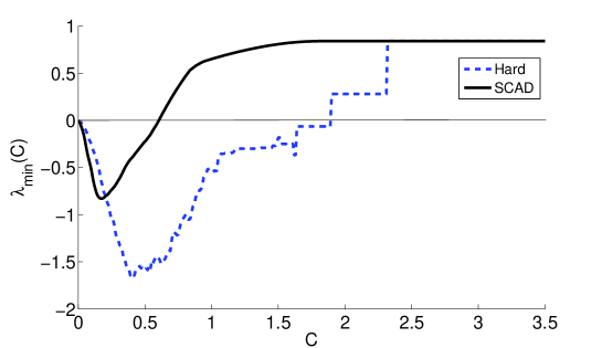
Data are simulated from the setting of Section 5 with . Both hard and SCAD with adaptive thresholds (Cai and Liu 2011) are plotted.
3.4 Asymptotic analysis
We now present the asymptotic analysis of the proposed two-step estimator. We first list a set of regularity conditions and then present the consistency. A more refined set of assumptions are needed to achieve the optimal rate of convergence as well as the limiting distributions.
3.4.1 Consistency
Assumption 3.1.
Let denote the th entry of . There is such that
In particular, when , we define , which corresponds to the “exactly sparse” case.
The first assumption sets a condition on the sparsity of , under which Fan et al. (2012) showed that the POET estimator is consistent under the operator norm. The sparsity is in terms of the maximum row sum, considered by Bickel and Levina (2008a).
The following assumption provides the regularity conditions on the data generating process. We introduce the strong mixing condition. Let and denote the -algebras generated by and respectively. In addition, define the mixing coefficient
| (3.3) |
Assumption 3.2.
(i)
is strictly stationary. In addition, for all and
(ii) There exist constants such that and .
(iii) Exponential tail: There exist and , such that for any , and ,
(iv) Strong mixing: There exists such that , and satisfying: for all ,
The following assumptions are standard in the approximate factor models, see e.g., Stock and Watson (1998, 2002) and Bai (2003). In particular, Assumption 3.3 implies that the first eigenvalues of are growing rapidly at . Intuitively, it requires the factors be pervasive in the sense that they impact a non-vanishing proportion of time series .
Assumption 3.3.
There is a such that for all large ,
Therefore all the eigenvalues of are bounded away from both zero and infinity as
Assumption 3.4.
There exists such that for all and ,
(i) ,
(ii) .
The following assumption defines the threshold on the th entry of for the step-one POET estimator.
Assumption 3.5.
The threshold where is entry-dependent, either stochastic or deterministic, such that , there are positive and so that
| (3.4) |
for all large and . Here is a deterministic constant.
Condition (3.4) requires the rate uniformly in . This condition is satisfied by the universal threshold for all , the correlation threshold as discussed before, and the adaptive threshold in Cai and Liu (2011).
For identification, we require the objective function be minimized subject to the diagonality of . In addition, since Assumption 3.3 is essential in asymptotically identifying the covariance decomposition , we need to take it into account when minimizing the objective function. Therefore we assume in Assumption 3.3 is sufficiently large, which leads to the following parameter space:
| (3.6) | |||||
Write and . We have the following theorem.
By a more careful large-sample analysis, we can improve the above result and derive the rate of convergence. Throughout the paper, we will frequently use the notation:
Remark 3.1.
In the above theorem does not need to be bounded. But in order to achieve the -consistency for each , the uniform rate of convergence above would require it be bounded (which is a strong assumption on the sparsity of ). Later in Section 3.4.3 we will enhance this convergence rate so that the boundedness of is not necessary and -consistency can still be achieved. This will require additional regularity conditions.
3.4.2 Covariance estimation and sparsistency
In order to obtain the limiting distribution for each individual , we also need to achieve the sparsistency for estimating By sparsistency, we mean the property that all small entries of are estimated as exactly zeros with a probability arbitrarily close to one. Besides being important for deriving the limiting distribution of , the sparsistency itself is of independent interest for large covariance estimation, and has been studied by many authors, for instance, Lam and Fan (2009) and Rothman et al. (2009). To our best knowledge, this is the first place where the sparsistency for an estimated idiosyncratic is achieved in a high dimensional approximate factor model.
Let and denote two disjoint sets and respectively include the indices of small and large elements of in absolute value, and
Because the diagonal elements represent the individual variances of the idiosyncratic components, we assume for all The sparsity assumes that most of the indices belong to when . A special case arises when is strictly sparse, in the sense that its elements in small magnitudes () are exactly zero. For the banded matrix as an example,
for some fixed Then and .
The following assumption quantifies the “small” and “big” entries of . By “small” entries we mean those of smaller order than The partition may not be unique. Our analysis suffices as long as such a partition exists.
Assumption 3.6.
There is a partition such that for all and is nonempty. In addition,
The conditional sparsity assumption requires most off-diagonal entries of be inside , hence it is reasonable to have in the condition. It is likely that only contains the diagonal elements. It then essentially corresponds to the strict factor model where is almost a diagonal matrix and error terms are only weakly cross-sectionally correlated. That is also a special case of Assumption 3.6.
Theorem 3.3.
It was shown by Fan et al. (2012) that . Theorem 3.4 below demonstrates a strengthened convergence rate for the averaged estimation error.
Assumption 3.7.
There is such that
In addition to Assumptions 3.1 and 3.6, we require the following condition on the sparsity of , which further characterizes and :
Assumption 3.8.
The index sets and satisfy: and .
Assumption 3.8 requires that the number of off-diagonal large entries of be of order , and that the absolute sum of the small entries is bounded. This assumption is satisfied, for example, if follows an heteroskedastic MA() process with a fixed , where and . It is also satisfied by banded matrices (Bickel and Levina 2008b, Cai and Yuan 2012) and block-diagonal matrices with fixed block size.
Define an matrix . Then implies
The following assumption corresponds to those of PCA in Bai (2003), and also extends to the non-diagonal .
Assumption 3.9.
(i)
(ii)
For each element of (),
,
(iii) For each element of ,
,
.
Under Assumption 3.9, we can achieve the following improved rate of convergence for the averaged estimation error :
Remark 3.2.
-
1.
A simple application of
by Fan et al. (2012) yields
In contrast, the rate we present in Theorem 3.4 requires more refined asymptotic analysis. It shows that after weighted by the factor loadings, the averaged convergence rate is faster. -
2.
The condition on the large-entry-set in Assumption 3.8 can be relaxed a bit to for an arbitrarily small , which will allow less sparse covariances. For example, Suppose follows a cross sectional AR() process such that
for and being independent across both and . We can then find a partition such that and for any Theorems 3.4 and 3.5 below still hold. But conditions in Assumption 3.9 need to be adjusted accordingly. For example, in condition (iii) the normalizing constant in the first equation should be changed to , and in the second equation should be changed to . The current Assumption 3.9, on the other hand, keeps our presentation simple.
3.4.3 Limiting distribution
As a result of Theorem 3.4, the impact of estimating at step one is asymptotically negligible. This enables us to achieve the -consistency and the limiting distribution of for each . We impose further assumptions.
Assumption 3.10.
(i) .
For each ,
(iii)
.
Theorem 3.5.
We make some technical remarks regarding Theorem 3.5.
Remark 3.3.
-
1.
The condition (roughly speaking, this is when is very large and ) strengthens the sparsity condition of Assumption 3.1. The required upper bound for is tight. Roughly speaking, the estimation error of plays a role in the asymptotic expansion of only through an averaged term as in Theorem 3.4. Condition is required for that term to be asymptotically negligible.
-
2.
The asymptotic normality also holds jointly for finitely many estimators. For any finite and fixed , we have,
where .
- 3.
3.4.4 Estimation of common factors
For the limiting distribution of , we make the following additional assumption:
Assumption 3.11.
There is a positive definite matrix such that for each
For the next assumption, we define . Then has mean zero and covariance matrix .
Assumption 3.12.
For any fixed ,
(i) ,
(ii) For each ,
Theorem 3.6.
Remark 3.4.
-
1.
It follows from Theorem 3.6 that for each fixed , is a root- consistent estimator of . Root- consistency for the estimated common factors also holds for the principal components estimator as in Bai (2003). In addition, the above limiting distribution holds only when
-
2.
If we strengthen the assumption to , then the uniform rate of convergence can be achieved:
To compare this rate with that of the PCA estimator, we consider for simplicity, the strictly sparse case . Then when and is either bounded or growing slowly (), the above rate is faster than that of the PCA estimator. (The above rate is when , whereas the uniform convergence rate for PCA estimator is )
4 Joint Estimation
4.1 - penalized maximum likelihood
One can also jointly estimate to take into account the cross-sectional dependence and heteroskedasticity simultaneously. As in the sparse covariance estimation literature (e.g., Lam and Fan 2009, Bien and Tibshirani 2011), we penalize the off-diagonal elements of the error covariance estimator, and minimize the following weighted- penalized objective function, motivated by a penalized Gaussian likelihood function:
| (4.1) | |||||
| (4.3) | |||||
where is the parameter space for , to be defined later. We introduce the weighted -penalty with to penalize the inclusion of many off-diagonal elements of in small magnitudes, which therefore produces a sparse estimator . Here is a tuning parameter that converges to zero at a not-too-fast rate; is an entry-dependent weight parameter, which can be either deterministic or stochastic. Popular choices of in the literature include:
- Lasso
-
The choice for all gives the well-known Lasso penalty studied by Tibshirani (1996). The Lasso penalty puts an equal weight to each element of the idiosyncratic covariance matrix.
- Adaptive-Lasso
-
Let be a preliminary consistent estimator of . Let for some , then
corresponds to the adaptive-lasso penalty proposed by Zou (2006). Note that the adaptive-lasso puts an entry-adaptive weight on each off-diagonal element of , whose reciprocal is proportional to the preliminary estimate. If the true element , the weight should be quite large, and results in a heavy penalty on that entry. The preliminary estimator can be taken, for example, as the PCA estimator . It was shown by Bai (2003) that under mild conditions, .
- SCAD:
-
Fan and Li (2001) proposed to use, for some (e.g, )
The notation stands for the positive part of ; is if , zero otherwise. Here is still a preliminary consistent estimator, which can be taken as the PCA estimator.
4.2 Consistency of the joint estimation
We assume the parameter space for to be, for some known sufficiently large ,
Then implies that all the eigenvalues of are bounded away from both zero and infinity. There are many examples where both the covariance and its inverse have bounded row sums. For example, for each , when follows a cross sectional autoregressive process AR for some fixed , then the maximum row sum of is bounded. The inverse of is a banded matrix, whose maximum row sum is also bounded.
As before we assume and be diagonal for identification. In addition, Assumptions 3.2 and 3.3 for the two-step estimation are still needed. Those conditions such as strong mixing, weakly dependence and bounded eigenvalues of regulate the data generating process, and asymptotically identify the covariance decomposition (2.1).
The conditions for the partition of are replaced by the following, which are weaker than those of two-step estimation in Assumption 3.8. Define the number of off-diagonal large entries:
| (4.4) |
Assumption 4.1.
There exists a partition where and are disjoint, which satisfies:
(i) for all ,
(ii)
(iii)
The following assumption is imposed on the penalty parameters. Define the weights ratios
Assumption 4.2.
The tuning parameter and the weights satisfy:
(i)
(ii)
The above assumption is not as complicated as it looks, and is satisfied by many examples. For instance, the Lasso penalty sets for all . Hence Then condition (i) of Assumption 4.2 follows from Assumption 4.1(ii), which is also satisfied if . Condition (ii) is also straightforward to verify. This immediately implies the following lemma.
Lemma 4.1 (Lasso).
Choose for all . Suppose in addition and . Then Assumption 4.2 is satisfied if the tuning parameter is such that
One of the attractive features of this lemma is that the condition on does not depend on the unknown We will present the adaptive lasso and SCAD as another two examples of the weighted- penalty in Section 4.3 below, both satisfy the above assumption.
Our main theorem is stated as follows.
Theorem 4.1.
Remark 4.1.
-
1.
The consistency for can be made uniformly in if the condition is strengthened to .
-
2.
To establish the consistency in the high dimensional literature, one usually constructs a neighborhood of the true parameters (e.g., Rothman et al. 2008, Lam and Fan 2009), and show that with probability approaching one, . This strategy however, does not work here due to the technical difficulty in dealing with the term in the likelihood function, because its largest eigenvalues are unbounded and grow at rate uniformly in the parameter space. One of the contributions of Theorem 4.1 is to achieve consistency using a new strategy to deal with the penalized likelihood function, which involves diverging eigenvalues.
In this paper we only present the consistency for the joint estimation, which is already technically difficult as one needs to deal with an equilibrium of the first order conditions for both simultaneously. Deriving the limiting distributions for the joint estimators is difficult, and we leave this as a future topic.
4.3 Two examples
We present two popular choices for the weights as examples: one is adaptive lasso, proposed by Zou (2006), and the other is SCAD by Fan and Li (2001). Both weights depend on a preliminary consistent estimate of each element of . In the high dimensional approximate factor model, a simple consistent estimate for each element can be obtained by the principal component analysis (Stock and Watson 1998 and Bai 2003).
To simplify the presentation, we will assume that , which controls the number of off-diagonal large entries of . Moreover, we retain Assumption 3.6:
and recall that .
Let the initial estimate , where is the PCA estimator of as in Bai (2003). The adaptive lasso chooses the weights to be, for some constant ,
| (4.5) |
where is a pre-determined nonnegative sequence. The additive was not included in the original definition of adaptive lasso in Zou (2006), but has often been seen in recent literature, e.g., Xue and Zou (2012). We include it here in the weights to prevent getting too large if is very close to zero. The adaptive lasso has been used extensively in the high dimensional literature, see for example, Huang, Ma and Zhang (2006), van de Geer, Bühlmann and Zhou (2011), Caner and Fan (2011), etc.
Another important example is SCAD, defined as: for some ,
| (4.6) |
We have the following theorem.
Theorem 4.2.
As in the case of Lemma 4.1, an attractive feature of this theorem is that, if both the upper bound of and the lower bound of
are known, [e.g., in the strictly sparse model,
, and assume is bounded away from zero as in MA(1)] then Conditions (4.7) - (4.9) do not depend on any other unknown feature of .
5 Numerical Examples
We propose a novel algorithm to numerically minimize the objective function (4.1) for joint estimation, which combines the EM algorithm with the majorize-minimize method recently proposed by Bien and Tibshirani (2011). The algorithm uses the PCA as initial values, and updates the estimator iteratively. At each iteration, an EM-algorithm is carried out to estimate and the empirical residual covariance Then a majorize-minimize method (Bien and Tibshirani 2011) is used to obtain a positive definite estimate of the covariance based on and soft-thresholding. The algorithm is summarized as follows (see Bai and Li (2012) and Bien and Tibshirani (2011) for detailed descriptions of the algorithm).
-
1.
Initialize and as the PCA estimators. Initialize as a diagonal matrix of the sample covariance based on the PCA residuals.
-
2.
At step k+1, , where
,Let
-
3.
Still at step , For some small value , let . Let
where and is a matrix whose off-diagonal is and diagonal elements are zero.
-
4.
Repeat 2-3 until converge.
We present a numerical experiment to illustrate the performance of the proposed method. The data was generated as following: are both serially and cross-sectionally independent as . Let
where are i.i.d. . Let the two factors be i.i.d. , and be uniform on . Then is a banded matrix.
We apply the adaptive lasso penalty for our joint estimation, with various choices of the tuning parameters and . The result is compared with the PCA estimator and the regular maximum likelihood restricted to diagonal (DML, Bai and Li 2012). More specifically, DML estimates by:
| (5.1) |
Therefore DML forces the covariance estimator to be diagonal even though the true is not. Hence it does not take the idiosyncratic cross-sectional dependence into account.
For each estimator, the smallest canonical correlation (the higher the better) between the estimator and the parameter has been used as a measurement to assess the accuracy of each estimator. Tables 1 and 2 list the results of the estimated factor loadings and common factors from joint-estimation.
| PCA | DML | Penalized ML | |||||
| 50 | 50 | 0.205 | 0.199 | 0.212 | 0.222 | 0.230 | 0.234 |
| 50 | 100 | 0.429 | 0.558 | 0.591 | 0.613 | 0.627 | 0.631 |
| 50 | 150 | 0.328 | 0.470 | 0.494 | 0.495 | 0.515 | 0.507 |
| 100 | 50 | 0.496 | 0.519 | 0.560 | 0.537 | 0.558 | 0.537 |
| 100 | 100 | 0.394 | 0.574 | 0.621 | 0.648 | 0.648 | 0.658 |
| 100 | 150 | 0.774 | 0.819 | 0.837 | 0.829 | 0.840 | 0.836 |
Canonical correlations are presented. DML is defined in (5.1) which treats to be diagonal. Penalized ML uses the one-step adaptive Lasso estimation.
| PCA | DML | Penalized ML | |||||
| 50 | 50 | 0.232 | 0.234 | 0.251 | 0.267 | 0.279 | 0.283 |
| 50 | 100 | 0.477 | 0.640 | 0.671 | 0.732 | 0.748 | 0.749 |
| 50 | 150 | 0.411 | 0.599 | 0.623 | 0.638 | 0.666 | 0.650 |
| 100 | 50 | 0.430 | 0.446 | 0.503 | 0.473 | 0.508 | 0.474 |
| 100 | 100 | 0.371 | 0.579 | 0.647 | 0.688 | 0.687 | 0.697 |
| 100 | 150 | 0.820 | 0.867 | 0.880 | 0.892 | 0.912 | 0.903 |
Canonical correlations are presented. Penalized ML uses the one-step adaptive Lasso estimation.
We have also computed the canonical correlations between the estimators and the true parameters using the regularized two-step method (Section 3) with iterations. For computational simplicity, the threshold value in the first step has been fixed to be the adaptive threshold of Fan et al. (2012) with a universal constant , which we find to maintain the finite-sample positive definiteness well. The results demonstrate that both two-step and joint estimations have higher canonical correlations, and thus outperform the PCA and DML.
Our EM plus majorize-minimize algorithm maximizes an approximate penalized likelihood function. Developing an efficient algorithm for maximizing the original likelihood function will be a future research direction.
| Factor loadings | Factors | ||||||
|---|---|---|---|---|---|---|---|
| PCA | DML | Two-step | PCA | DML | Two-step | ||
| ML | ML | ||||||
| 50 | 50 | 0.205 | 0.199 | 0.241 | 0.232 | 0.234 | 0.277 |
| 50 | 100 | 0.429 | 0.558 | 0.643 | 0.477 | 0.640 | 0.752 |
| 50 | 150 | 0.328 | 0.470 | 0.565 | 0.411 | 0.599 | 0.731 |
| 100 | 50 | 0.496 | 0.519 | 0.548 | 0.430 | 0.446 | 0.469 |
| 100 | 100 | 0.394 | 0.574 | 0.717 | 0.371 | 0.579 | 0.758 |
| 100 | 150 | 0.774 | 0.819 | 0.846 | 0.820 | 0.867 | 0.927 |
The SCAD threshold has been used for the covariance estimation, where with the adaptive threshold constant proposed by Cai and Liu (2011).
6 Conclusion
We study the estimation of a high dimensional approximate factor model in the presence of cross sectional dependence and heteroskedasticity. The classical PCA method does not efficiently estimate the factor loadings or common factors because it essentially treats the idiosyncratic error to be homoskedastic and cross sectionally uncorrelated. For the efficient estimation it is essential to estimate a large error covariance matrix.
We assume the model to be conditionally sparse in the sense that after the common factors are taken out, the idiosyncratic components have a sparse covariance matrix. This enables us to combine the merits of both sparsity and high dimensional factor analysis. Two maximum-likelihood-based approaches are proposed to estimate the common factors and factor loadings, both involve regularizing a large covariance sparse matrix. Extensive asymptotic analysis has been carried out. In particular, we develop the inferential theory for the two-step estimation.
It remains to derive the limiting distribution as well as the optimal rates of convergence for the estimators by the joint-estimation method. This will extend the consistency results obtained in the current paper. In the presence of a covariance that has fast-diverging eigenvalues, the task is difficult because it requires the consistency of the penalized covariance estimator under the operator norm. We intend to address this issue in future research.
Appendix A Proofs for generic estimators
We need to establish the results for two sets of estimators: the two-step estimator and the joint estimator, whose proofs for consistency share some similarities. Therefore in this section we establish some preliminary results for generic estimators that can be used for both cases. We denote by as a generic estimator for , which can be either or . Define
| (A.1) |
| (A.2) |
Define the set
We first present a lemma that will be needed throughout the proof.
Lemma A.1.
(i) .
(ii) .
(iii) .
Proof.
See Lemmas A.3 and B.1 in Fan, Liao and Mincheva (2011). ∎
Lemma A.2.
Under Assumption 3.2, for any ,
Therefore we can write
| (A.3) | |||
| (A.4) |
Proof.
First of all, note that , and hence we have
| (A.5) |
where is uniform in . Equation (A.5) will be used later in the proof.
We now consider the term . With the identification condition and ,
By the matrix inversion formula ,
| (A.6) |
where , and Term uniformly in the parameter space, and hence can be ignored.
Let us look at terms and subsequently. Note that and are both bounded from above uniformly in , we have,
| (A.7) |
| (A.8) |
In addition, , uniformly in , and . Applying the matrix inversion formula yields
| (A.9) | |||||
| (A.10) |
where is uniform over . In the second equality above we applied (A.7) and (A.8) and the following inequality:
By Lemma A.1(iii), and uniformly in ,
| (A.11) |
Similarly, Again by the matrix inversion formula,
The second term on the right hand side is of smaller order (uniformly) than the first term, because it has an additional term , whose maximum eigenvalue is uniformly by (A.8). The first term is bounded by (uniformly in ):
Hence Results (A.5) and (A.6) then yield
∎
Throughout the proofs, we note that the consistency depends crucially on the consistency of the following quantities:
We state the following lemma for the generic estimators.
Lemma A.3.
(i)
(ii) First order condition:
We will prove Lemma A.3 for both and later when we deal with these two estimators individually.
Lemma A.4.
Suppose Lemma A.3 holds, then
(i)
(ii)
Proof.
(i) Using the matrix inverse formula, the same argument of Bai and Li (2012)’s (A.2) implies . Thus part (i) follows from the first order condition in Lemma A.3.
(ii) Let . Part (i) can be equivalently written as where
Note that for , , for each element, , , hence
Moreover, for the empirical covariance by Lemma A.1, which implies . Also, . Therefore It then implies (ii).
∎
Lemma A.5.
Suppose Lemma A.3 holds, then .
Proof.
By our assumption, both and are diagonal. Moreover, the eigenvalues of and are bounded away from zero. Therefore by Lemma A.3(i) and Lemma A.4(ii), there are two diagonal matrices and whose eigenvalues are all bounded away from zero, such that
| (A.12) |
Applying Lemma A.1 of Bai and Li (2012), we have and . We also assumed and have the same column signs, as a part of identification condition.
∎
Appendix B Proofs for Section 3
In this section, and Throughout Appendix B, we will let . For notational simplicity, we let
We first cite a result from Fan et al. (2012):
Theorem B.1 (Theorem 3.1 in Fan et al. (2012)).
Suppose and , then under Assumptions 3.1- 3.5,
Proof.
The sufficient conditions of this theorem are satisfied by our assumptions. See Fan et al. (2012). ∎
We then prove Lemma A.3, which then enables us to apply Lemmas A.4 and A.5. Under Assumptions 3.1- 3.3, there is such that and with probability approaching one for in Appendix A.
Lemma B.1.
For , Lemma A.3 is satisfied.
Proof.
The first order condition with respect to in (ii) is easy to verify, which is the same as that in Bai and Li (2012). We only show part (i).
By definition, . Also the representation defined in Lemma A.2 yields
Thus
Note that is always nonnegative and . Therefore by Lemma A.2, . Moreover, the matrix in the trace operation of is semi-positive definite, hence
| (B.1) |
It remains to show that , which follows immediately from Theorem B.1 and that .
∎
B.1 Proof of Theorem 3.1
B.1.1 Consistency for
B.1.2 Consistency for
Lemma A.4 (i) can be equivalently written as: for any ,
| (B.2) |
where denotes the th column of , and is an vector
The consistency of follows from Lemma A.5 and the following Lemma B.2.
Lemma B.2.
Proof.
By Lemma A.1, uniformly in ,
Finally, . The result then follows from a triangular inequality and that . ∎
B.2 Proof of Theorem 3.2
B.2.1 Uniform rate for
Lemma B.3.
.
Proof.
The first order condition in Lemma A.4 (i) is equivalent to:
| (B.3) |
where We have, , , and Therefore Since , can be ignored. It follows from (B.3) that
| (B.4) |
Let denote the the entry of . It then follows that for all It is also not hard to verify that for any since .
On the other hand, due to the identification condition, both and are diagonal. Let ndg denote the off-diagonal elements of . Then ndgndg is equivalent to
Note that if then for two matrices and since is diagonal. Also, . The above identification condition implies
| (B.5) |
Note that Let denote the th diagonal entry of . Let . Then for , (B.4) and (B.5) imply that
By assumption, with probability one, there is such that , and for Moreover, since all the eigenvalues of are bounded away from zero and infinity, wpa1, for some Then the above two equations imply that for any , (since ). Then
| (B.6) |
Moreover, by Lemma B.2, .
We now show that . Suppose this does not hold, then (B.6) implies . By the definition
. Therefore yields . The first order condition (B.2) also yields
which implies . Therefore
which contradicts with the consistency . This concludes the proof.
∎
Therefore, (B.2) gives . The rate of convergence for then follows immediately since it is bounded by .
B.3 Proof of Theorem 3.3
By the definition of the covariance estimator in the first step, , where is a chosen thresholding function. It was shown by Fan et al. (2012, Theorem 2.1) that is the PCA estimator of , that is, .
Lemma B.4.
For any , and any constant , for all large enough ,
Proof.
We have, . Thus for all large enough ,
where in the second and last inequalities we used the assumption that and the fact that .
∎
Proof of Theorem 3.3
By Fan et al. (2012), , which implies for any , there is such that . For some universal , we set the threshold at entry , where is a data-dependent value that satisfies, for any , there is such that Then as long as the constant in the definition of the threshold is larger than ,
Note also that if , then , by the definition of . This implies,
Since by assumption, for all large
On the other hand, for arbitrarily small , for some , which implies By the definition of , for all . Therefore , hence for arbitrarily large ,
where the last inequality follows from Lemma B.4.
B.4 Proof of Theorems 3.4 and 3.5
B.4.1 Proof of Theorem 3.4
A simple derivation implies that . This rate is not tight enough for the -consistency and limiting distribution . A more refined rate of depends on the convergence properties of the PCA estimator. We begin by citing some results proved by Fan et al. (2012). Recall that denotes the th entry of the orthogonal complement covariance in the sample covariance’s spectrum decomposition, and
Let be the PCA estimates of . Let and denote the PCA estimators of the factor loadings and factors.
Lemma B.5.
(i) For any , with probability one ,
(ii)
(iii) There is a nonsingular matrix such that and
(iv)
Proof.
See Theorem 2.1 and Lemma C.11 of Fan et al. (2012). ∎
Lemma B.6.
.
Proof.
By Bai (2003), there are two matrices and , , such that . The desired result then follows from the following Lemma B.7.
∎
Lemma B.7.
(i)
(ii)
(iii) .
Proof.
(i) We have,
| (B.7) | |||
| (B.8) |
We bound separately. Here is upper bounded by , where by Cauchy-Schwarz,
| (B.9) | |||||
| (B.10) | |||||
| (B.11) |
Note that , which is by Assumption 3.9. Hence .
| (B.12) |
Since by the strong mixing condition (Lemma C.5 of Fan Liao and Mincheva 2012), we have . This implies .
Now we bound . Using Cauchy Schwarz inequality, we have where
| (B.14) | |||||
| (B.15) |
where the second inequality follows from . Using Cauchy-Schwarz inequality, we also obtain
| (B.16) | |||||
| (B.17) | |||||
| (B.18) |
(ii) Let be the th element of . Then the th element of the object of interest is bounded by , where, by Cauchy Schwarz inequality,
| (B.19) | |||||
| (B.20) | |||||
| (B.21) |
The last equality follows from Assumption 3.9. Also, . Thus
| (B.22) | |||||
| (B.23) |
(iii) The object of interest is bounded by , where
| (B.24) |
and we used the fact that from Lemma B.5, and that 111We have , whose expectation is . Note that uniformly in .
| (B.25) |
∎
Lemma B.8.
For in the partition ,
(i)
(ii)
(iii) .
Proof.
(i) The term of interest is bounded by , where
Here is upper bounded by , where
, and
Note that and can be bounded in the same way as (B.9) and (B.12). The only difference is that is replaced by a double sum . By the assumption, . The result of the proof is exactly the same, so is omitted.
We conclude that .
On the other hand, where
, and
. Using Cauchy-Schwarz inequality and the strong mixing condition, and can be also bounded in an exactly the same way of (B.14) and (B.16). We conclude that .
(ii) Let be the th element of . Then the th element of the object of interest is bounded by , where
, and
. Bounding is slightly different from (B.19) and (B.22), and we give the detail here. By Cauchy Schwarz inequality,
which is by Assumption 3.9. On the other hand,
. Note that , where is as defined in Assumption 3.1. Thus .
(iii) The object of interest is bounded by , where
.
Since , we conclude that , and . ∎
From Lemma B.8, immediately we have the following result.
Lemma B.9.
.
Proof.
The following lemma strengthens the results of Bai (2003) when is sparse.
Lemma B.10.
For the PCA estimator,
(i)
(ii) .
Proof.
(i) . By Assumption 3.9, On the other hand, is equal to
The first term on the right hand side is . We now work on the second term. By Bai (2003), there is a nonsingular matrix such that
| (B.26) |
By Lemma B.6 In addition, for each element of ,
which is Also,
(ii) Since , the term of interest equals
By Assumption 3.9, the third term is . By the assumption that and Cauchy Schwarz inequality, the second term is . We now work out the first term. Again we use the equality . Lemma B.9 gives
On the other hand, is bounded by,
since . Also, is bounded by
which is .
∎
Proof of Theorem 3.4
Proof.
By the triangular inequality, the left-hand-side is bounded by
The first term is . We now bound the second term, which is
where The first term on the right hand side is by Lemma B.10. The third term is dominated by, By Theorem 3.3, for any and any , This implies the third term is The second term equals
By Lemma B.10 (ii), On the other hand, recall that when (Section 3.1),
Write , then for any , and , Lemma B.4 implies , which yields . Therefore . This implies .
∎
B.4.2 Convergence rate for
We now improve the rate in Lemma B.3.
Lemma B.11.
(i)
(ii)
Proof.
(i) By Theorem 3.2,
| (B.27) |
Therefore the RHS of part (i) equals
| (B.28) |
Now it follows from Assumption 3.10 that
which then yields the desired result.
(ii) Recall that and that
∎
Lemma B.12.
.
B.4.3 Improved rate for
Lemma B.13.
(i) .
(ii)
Proof.
(i) We have, . Hence Hence part (i) equals
where is uniform in By Assumption 3.10, for each ,
(ii) We have . Hence (ii) equals
By Assumption 3.10, the first term equals , which yields the desired result. ∎
Lemma B.14.
For each fixed ,
B.4.4 Proof of Theorem 3.5
B.5 Proof of Theorem 3.6
For any , . Hence
| (B.29) |
B.5.1 Convergence rate
Since both and have exponential tails, using Bonferroni’s method we have, and . Thus by Lemma B.12, . The term with in (B.29) is of smaller order hence is negligible. Also , where we used . Hence
Finally, because , whose eigenvalues are bounded. Hence . Also, is of smaller order than
. This implies
The above proof also shows that the rate can be made uniform if
B.5.2 Asymptotic normality
Recall that and .
Lemma B.15.
For any fixed , .
Proof.
We expand using the first order condition
| (B.30) |
and investigate each term separately. First of all, since , and by assumption that , we have Second, by the assumption that , we have
Third, Moreover,
. Therefore, by the assumption that , we have,
Finally, ∎
Lemma B.16.
For any fixed ,
Proof.
Proof of asymptotic normality
Appendix C Proofs of Section 4
C.1 Proof of Theorem 4.1
Define
Let . Then the minimizer of is the same as that of This implies . Recall the definitions of and Then
Lemma C.1.
There is a nonnegative stochastic sequence such that with probability one.
Proof.
We have . In addition, . Hence
By the definition of , there is such that The result then holds for by Lemma A.2.
∎
Throughout, let (recall that )
Lemma C.2.
For all large enough and ,
Proof.
Let , . For any , let . Define a function , Then and
| (C.1) |
By the integral remainder Taylor expansion, . We now calculate and . Using the matrix differentiation formula, we have, which implies,
Note that both and are bounded from above for . By Lemma A.1(ii), Therefore, . In addition,
where dentoes the vectorization operator and denotes the Kronecker product. Since both and are inside , is bounded from above, which then implies is bounded below by a positive constant . Hence From (C.1) and , we have
Since , and . It follows that
which implies the desired result. ∎
Lemma C.3.
Proof.
Lemma C.2 implies
Lemma C.1 gives Hence we have
Note that . Hence the desired result follows from wp1 and .
∎
Lemma C.4.
Lemma C.5.
Proof.
Let , , and . Since the norms of and are bounded away from infinity, we have, and . Then
The first term on the right hand side is by Lemma C.4, and the second is bounded by (using Cauchy-Schwarz inequality), which is also by Lemma C.3 and Assumption 4.2.
∎
Lemma C.6.
For , Lemma A.3 is satisfied.
Proof.
We first show part (i) of Lemma A.3. Since , and , there is a nonnegative sequence such that Lemma C.2 then implies . On the other hand,
The matrix in the bracket is semi-positive definite. Hence
| (C.2) |
Finally, the desired result follows from Lemma C.5.
The first order condition in part (ii) is easy to derive and is the same as that in Bai and Li (2012).
∎
Proof of Theorem 4.1
C.2 Proof of Theorem 4.2
We now verify Assumption 4.2 for the Adaptive Lasso.
Lemma C.7.
For adaptive lasso,
(i) .
(ii) ,
(iii) (recall that ).
Proof.
By Lemma B.5 Given this result and the assumption that , we have result (i). For any , the following inequality holds: which then implies results (ii) and (iii), due to the assumptions that , and ∎
Proof of Assumption 4.2 for Adaptive Lasso
It follows from the previous lemma that and . By the assumption that ,
Hence . This together with the lower bound assumption on yields Assumption 4.2 (i).
For part (ii), note that implies that with probability approaching one,
By Lemma C.7(ii), (recall that ) and the lower bound ,
By Lemma C.7(i) and the assumptions that and we have due to the upper bound on Finally, by Lemma C.7(iii) and the assumption that , we have
Proof of Assumption 4.2 for SCAD
Since and , it is easy to verify that with probability approaching one, , . Hence and This immediately implies the desired result.
References
- 1 Alessi, L., Barigozzi, M. and Capassoc, M. (2010). Improved penalization for determining the number of factors in approximate factor models. Statistics and Probability Letters, 80, 1806-1813.
- 2 Bai, J. (2003). Inferential theory for factor models of large dimensions. Econometrica. 71 135-171.
- 3 Bai, J. and Li, K. (2012). Statistical analysis of factor models of high dimension. Ann. Statist. 40, 436-465.
- 4 Bai, J. and Ng, S.(2002). Determining the number of factors in approximate factor models. Econometrica. 70 191-221.
- 5 Bickel, P. and Levina, E. (2008a). Covariance regularization by thresholding. Ann. Statist. 36 2577-2604.
- 6 Bickel, P. and Levina, E. (2008b). Regularized estimation of large covariance matrices. Ann. Statist. 36 199-227.
- 7 Bien, J. and Tibshirani, R. (2011). Sparse estimation of a covariance matrix. Biometrika. 98, 807-820.
- 8 Breitung, J. and Tenhofen, J. (2011). GLS estimation of dynamic factor models. J. Amer. Statist. Assoc. 106, 1150–1166.
- 9 Cai, T. and Liu, W. (2011). Adaptive thresholding for sparse covariance matrix estimation. J. Amer. Statist. Assoc. 106, 672-684.
- 10 Cai, T. and Yuan, M. (2012). Adaptive covariance matrix estimation through block thresholding. Forthcoming in Ann. Statist.
- 11 Cai, T. and Zhou, H. (2012). Optimal rates of convergence for sparse covariance matrix estimation. Forthcoming in Ann. Statist.
- 12 Caner, M. and Fan, M. (2011). A near minimax risk bound: adaptive lasso with heteroskedastic data in instrumental variable selection. Manuscript. North Carolina State University.
- 13 Chamberlain, G. and Rothschild, M. (1983). Arbitrage, factor structure and mean-variance analysis in large asset markets. Econometrica. 51 1305-1324.
- 14 Choi, I. (2012). Efficient estimation of factor models. Econometric Theory. 28 274-308.
- 15 Deng, X. and Tsui, K. (2010). Penalized covariance matrix estimation using a matrix-logarithm transformation. Manuscript, University of Wisconsin-Madison
- 16 Dias, F., Pinherio, M. and Rua, A. (2008). Determining the number of factors in approximate factor models with global and group-specific factors. Manuscript. Technical University of Lisbon.
- 17 Fan, J., Fan, Y. and Lv, J. (2008). High dimensional covariance matrix estimation using a factor model. J. Econometrics. 147, 186-197.
- 18 Fan, J. and Li, R. (2001). Variable selection via nonconcave penalized likelihood and its oracle properties. J. Amer. Statist. Assoc. 96 1348-1360
- 19 Fan, J., Liao, Y. and Mincheva, M. (2012). Large covariance estimation by thresholding principal orthogonal complements. Manuscript. Princeton University.
- 20 Forni, M., Hallin, M., Lippi, M. and Reichlin, L. (2000). The generalized dynamic factor model: identification and estimation. Review of Economics and Statistics. 82 540-554.
- 21 Forni, M. and Lippi, M. (2001). The generalized dynamic factor model: representation theory. Econometric Theory. 17 1113-1141.
- 22 van de Geer, S., Bühlmann, P. and Zhou, S. (2011). The adaptive and the thresholded Lasso for potentially misspecified models (and a lower bound for the Lasso). Electronic Journal of Statistics. 5, 688-749.
- 23 Hallin, M. and Liška, R. (2007). Determining the number of factors in the general dynamic factor model. J. Amer. Statist. Assoc. 102, 603-617.
- 24 Han, X. (2012). Determining the number of factors with potentially strong cross-sectional correlation in idiosyncratic shocks. Manuscript. North Carolina State University
- 25 Huang, J., Ma, S. and Zhang, C. (2006). Adaptive lasso for sparse high-dimensional regression models. Manuscript. University of Iowa.
- 26 Johnstone, I.M. and Lu, A.Y. (2009). On consistency and sparsity for principal components analysis in high dimensions. Jour. Ameri. Statist. Assoc., 104, 682-693.
- 27 Jung, S. and Marron, J.S. (2009). PCA consistency in high dimension, low sample size context. Ann. Statist., 37, 4104-4130.
- 28 Kapetanios, G. (2010). A testing procedure for determining the number of factors in approximate factor models with large datasets. Journal of Business and Economic Statistics. 28, 397-409.
- 29 El Karoui, N. (2008). Spectrum estimation for large dimensional covariance matrices using random matrix theory. Ann. Statist. 36 2757-2790.
- 30 Lam, C. and Fan, J. (2009). Sparsistency and rates of convergence in large covariance matrix estimation. Ann. Statist. 37 4254-4278.
- 31 Lam, C. and Yao, Q. (2012). Factor modelling for high-dimensional time series: inference for the number of factors. Forthcoming in Ann. Statist.
- 32 Lawley, D. and Maxwell, A. (1971). Factor analysis as a statistical method. Second ed. London, Butterworths.
- 33 Ledoit, O. and Wolf, M. (2012). Nonlinear shrinkage estimation of large-dimensional covariance matrices. Ann. Statist. 40, 1024-1060.
- 34 Onatski, A. (2010). Determining the number of factors from empirical distribution of eigenvalues. The Review of Economics and Statistics. 92, 1004-1016.
- 35 Pati, D., Bhattacharya, A., Pillai, N. and Dunson, D. (2012) Posterior contraction in sparse Bayesian factor models for massive covariance matrices. Manuscript, Duke University
- 36 Ravikumar, P., Wainwright, M., Raskutti, G. and Yu, B. (2011), High-dimensional covariance estimation by minimizing -penalized log-determinant divergence, Electronic Journal of Statistics. 5 935-980.
- 37 Rohde, A. and Tsybakov, A. (2011), Estimation of high-dimensional low-rank matrices. Ann. Statist. 39 887-930.
- 38 Rothman, A., Levina, E. and Zhu, J. (2009). Generalized thresholding of large covariance matrices. J. Amer. Statist. Assoc. 104 177-186.
- 39 Stock, J. and Watson, M. (1998). Diffusion Indexes, NBER Working Paper 6702.
- 40 Stock, J. and Watson, M. (2002). Forecasting using principal components from a large number of predictors. J. Amer. Statist. Assoc. 97, 1167-1179.
- 41 Tibshirani, R. (1996). Regression shrinkage and selection via the Lasso. Journal of the Royal Statistical Society, Ser. B, 58 267-288
- 42 Wang, P. (2009). Large dimensional factor models with a multi-level factor structure: identification, estimation and inference. Manuscript. Hong Kong University of Science and Technology.
- 43 Witten, D.M., Tibshirani, R. and Hastie, T. (2009). A penalized matrix decomposition, with applications to sparse principal components and canonical correlation analysis. Biostatistics, 10, 515-534.
- 44 Xue, L. and Zou, H. (2012). Regularized rank-based estimation of high-dimensional nonparanormal graphical models. Forthcoming in Ann. Statist.
- 45 Yuan, M. (2010). High dimensional inverse covariance matrix estimation via linear programming. J. Machine Learning Research. 2010, 2261-2286
- 46 Zhang, C. (2010). Nearly unbiased variable selection under minimax concave penalty, Ann. Statist., 38 894-942
- 47 Zhou, S., Rütimann, P., Xu, M. and Bühlmann, P. (2011), High-dimensional covariance estimation based on Gaussian graphical models. Journal of Machine Learning Research. 12, 2975-3026.
- 48 Zou, H. (2006). The adaptive Lasso and its oracle properties. J. Amer. Statist. Assoc. 101 1418-1429