Global gyrokinetic particle-in-cell simulations of internal kink instabilities

Abstract

Internal kink instabilities have been studied in straight tokamak geometry employing an electromagnetic gyrokinetic particle-in-cell (PIC) code. The ideal-MHD internal kink mode and the collisionless $m=1$ tearing mode have been successfully simulated with the PIC code. Diamagnetic effects on the internal kink modes have also been investigated.

I Introduction

The internal kink instability is a fluid fixed-boundary mode which can, however, be strongly affected by kinetic effects. It occurs if the safety factor $q(r_{c})=1$ at some position $r_{c}$ inside the plasma column Newcomb_60 ; Shafranov_70 ; Rosenbluth73 . The fluid internal kink mode is always unstable in screw pinch geometry, but it can be partially stabilized by toroidal corrections Bussac75 . Nevertheless, it plays an important role in tokamak operation (in particular during “sawtooth” sawteeth_ST and “fishbone” fishbones_PDX activity). In the fluid picture, the internal kink mode is destabilized by the gradients of the parallel current and of the plasma pressure. Physically, the kink instability is a tilt and a shift of the plasma column. It can be unstable because the field line bending vanishes at the position $r_{c}$ and fails to compensate the magnetic force associated with the gradient of the ambient parallel current and the gradient of the pressure (directly related to the diamagnetic current). The uncompensated perturbed magnetic energy is then set free in the narrow “inertial” (or “resonant”) layer around $r_{c}$ and is converted to kinetic energy of poloidally rotating plasma (and drives reconnection when non-ideal effects are important). A kinetic description may be needed in order to address the physics of the inertial (resonant) layers.

The internal kink instability has been known in plasma physics research from the beginning of the fusion programme. Already in 1973, it was considered as a plausible candidate to explain the $q(0)>1$ tokamak stabilitiy criterion. It has been hypothesized Rosenbluth73 that the internal kink mode can be involved in the disruptive instabilities. In Ref. Rosenbluth73 , an ideal Magnetohydrodynamical (MHD) theory of the internal kink modes was developed. A nonlinear kinked neighboring equilibrium was found. However, the resulting nonlinear ideal-MHD amplitudes were too small to explain the disruptive phenomena in tokamaks although such qualitative properties as the negative voltage spikes and inward shifts in major radius produced by the mode evolution agreed with the experimental observations. The next time the internal kink modes received increased attention was in 1975 when B. Kadomtsev proposed his model Kadomtsev_sawteeth for the sawtooth phenomena, discovered experimentally one year before sawteeth_ST . In this model, the growth of the magnetic island associated with the internal kink mode (poloidal mode number $m=1$) plays a crucial role. Clearly, such a process is beyond the range of the ideal MHD theory considered in Rosenbluth73 .

This has motivated the development of theoretical descriptions of the internal kink mode which include various non-ideal effects. Thus, in Ref. Ara77 the internal kink mode has been considered within a two-fluid model including resistivity, ion-ion collisions and diamagnetic effects (which were found to be stabilizing). Further development focused on a more detailed description of the resonant layer around the $q=1$ magnetic surface. In Ref. Drake78 , the kinetic theory of the $m=1$ internal instability was considered (kinetic electrons and fluid ions). Similarly to Ref. Ara77 , a diamagnetic stabilization of the internal kink mode was found. In Ref. BasuCoppi80 , the role of collisionless reconnection (driven by the electron inertia) on the evolution of the internal kink mode was studied in the regime $\delta_{e}\gg\rho_{i}$ (here $\delta_{e}$ is the electron skin depth and $\rho_{i}$ is the ion gyroradius), neglecting ion Finite Larmor Radius (FLR) effects. Such a regime corresponds to very low values of plasma pressure $\beta\leq m_{e}/m_{i}$. It has been pointed out, however, that an accurate treatment of the ion orbits (in terms of their gyro-average) is needed in order to consider realistic regimes with $\delta_{e}\leq\rho_{i}$. A technical difficulty arising here is due to the non-local character of the gyrokinetic polarization density which results in an integral quasineutrality equation (see also Antonsen81 ). This problem has been addressed in Ref. Cowley86 in the context of the tearing mode problem. The integral equation resulting from the non-local ion response has been solved by an iterative method (assuming the poloidal beta to be small). In Ref. PegoraroSchep89 , an alternative approach to this problem has been suggested based on the Fourier expansion in the resonant layer with respect to the radial variable. This approach emphasizes the singular layer but retains the global nature of the mode through the boundary conditions. An interpolation formula has been used in order to treat the gyro-averages (it fails when the density or temperature gradients are too large). In 1991, Porcelli combined the approach of Ref. PegoraroSchep89 concerning the ions with electron inertia effects assuming, however, an adiabatic or isothermal electron temperature response (depending on the parameter regime). In Ref. Porcelli91 , he found the so-called $m=1$ collisionless tearing mode which dominates the ideal-MHD version of the internal kink mode when the ideal drive is sufficiently small (basically, when the ion gyroradius exceeds the ideal-MHD inertial length). This development has been used in the formulation of the revised sawtooth model Porcelli_sawteeth by Porcelli et al in 1996 (this model takes into account the complex dynamics of the resonant layer which includes the ion FLR and reconnection effects).

Despite the great progress achieved in the analytical understanding of internal kink modes, it is still an area of active research. Thus, very recently a unified theory of the internal kink and tearing modes has been developed in Ref. Zocco2012 . This theory provides an accurate treatment of the ion orbits and the electron temperature response without assuming it to be adiabatic or isothermal.

On the numerical side, there is a vast literature on simulations of internal kink modes using the fluid approach. For example, Ref. Martynov05 analyzes the ideal stability of the internal kink mode in shaped tokamak plasmas. Recent full-MHD simulations Halpern11_PPCF ; Halpern11_PoP studied various nonlinear regimes of the internal kink mode evolution and included some two-fluid (e. g. diamagnetic) effects. It is however desirable to have a first principles approach to the internal kink mode since the kinetic effects can be important in the resonant layer, and two-fluid models are often derived under a number of assumptions that may be too simplistic. Such an attempt was undertaken for the first time with a gyrokinetic Brizard:nonlin_gyrokin_finite_beta particle-in-cell Lee code in 1995. In Ref. SydoraNaitou95 , both the linear and nonlinear evolution of the internal kink mode were simulated, targeting the sawtooth collapse on a fast time scale. However, these early simulations operated at extremely small $\beta\leq m_{e}/m_{i}$ and neglected ion FLR effects. This work has recently been continued in Ref. Naitou2009 (also at a very small plasma beta). In addition to particle-in-cell simulations, the internal kink mode has been considered by employing an eigenvalue approach to the solution of the gyrokinetic equations Qin:gyrokin_perp_dynamic ; Lauber_phd .

In this paper, we study the linear evolution of the internal kink mode in straight-tokamak geometry employing the global gyrokinetic particle-in-cell method. Realistic values of plasma $\beta\gg m_{e}/m_{i}$ are used. The objective of this paper is two-fold. First, we study how the kink mode properties change depending on the relation between the ion gyroradius and the MHD inertial length. Second, we explore, for the first time, what could be the limitations of the gyrokinetic PIC approach to this problem at realistic values of plasma beta.

The structure of the paper is as follows. In Sec. II, the basic equations and the discretization procedure are discussed. Simulations in the fluid and kinetic regimes are presented in Sec. III. Finally, our conclusions are summarized in Sec. IV.

II Basic equations and numerical approach

We use the linear two-dimensional $\delta f$ PIC-code GYGLES Mishchenko_tae ; Mishchenko_fast ; Mishchenko_bulk . The code is electromagnetic and treats all particle species (ions and electrons) kinetically. It solves the gyrokinetic Vlasov-Maxwell system of equations (in the $p_{\|}$-formulation, see Ref. Brizard:nonlin_gyrokin_finite_beta for details). The distribution function is split into a background part and a small time-dependent perturbation $f_{s}=F_{0s}+\delta f_{s}$ (the index $s=i,e$ is used for the particle species). The background ion distribution function is taken to be a Maxwellian. The background electron distribution function is a shifted Maxwellian (to account for the equilibrium parallel current):

$$F_{0e}=n_{0}\left(\frac{m}{2\pi T_{e}}\right)^{3/2}\exp\left[{}-\frac{m_{e}(p_{\|}-u)^{2}}{2T_{e}}\right]\exp\left[{}-\frac{m_{e}v_{\perp}^{2}}{2T_{e}}\right]$$ (1)

Here $u={}-j_{\|}^{(0)}/(en_{0})$ and $\mu_{0}\,j_{\|}^{(0)}=({\bf{B}}/B)\cdot(\nabla\times{\bf{B}})$ with ${\bf{B}}$ the equilibrium magnetic field.

Assuming the amplitude of the field perturbation to be small (this implies $\delta f_{s}/F_{0s}\ll 1$), the first-order perturbed distribution function can be found from the linearized Vlasov equation:

$${\frac{\partial\delta f_{s}}{\partial t}}+\dot{{\bf{R}}}^{(0)}\cdot{\frac{\partial\delta f_{s}}{\partial{\bf{R}}}}+\dot{p}_{\|}^{(0)}{\frac{\partial\delta f_{s}}{\partial p_{\|}}}={}-\dot{{\bf{R}}}^{(1)}\cdot{\frac{\partial F_{0s}}{\partial{\bf{R}}}}-\dot{p}_{\|}^{(1)}{\frac{\partial F_{0s}}{\partial p_{\|}}}.$$ (2)

Here, $[\dot{{\bf{R}}}^{(0)},\dot{p}_{\|}^{(0)}]$ correspond to the unperturbed gyrocenter position and parallel velocity, and $[\dot{{\bf{R}}}^{(1)},\dot{p}_{\|}^{(1)}]$ are the perturbations of the particle trajectories proportional to the electromagnetic field fluctuations [shown in Eqs. (4)-(7) below]. The perturbed part of the distribution function is discretized with markers (see Ref. Fivaz_1998 for details):

$$\delta f_{s}({\bf{R}},p_{\|},\mu,t)=\sum_{\nu=1}^{N_{p}}w_{s\nu}(t)\delta({\bf{R}}-{\bf{R}}_{\nu})\delta(p_{\|}-p_{\|\nu})\delta(\mu-\mu_{\nu})\ ,$$ (3)

where $N_{p}$ is the number of markers, $({\bf{R}}_{\nu},p_{\|\nu},\mu_{\nu})$ are the marker phase space coordinates and $w_{s\nu}$ is the weight of a marker. The equations of motion are Brizard:nonlin_gyrokin_finite_beta

$${\bf{\dot{R}}}^{(0)} = p_{\|}{\bf{b}}^{*}+\frac{1}{qB_{\|}^{*}}{\bf{b}}\times\mu\nabla B$$ (4)

$${\bf{\dot{R}}}^{(1)} = {}-\frac{q}{m}\langle A_{\|}\rangle{\bf{b}}^{*}+\frac{1}{B_{\|}^{*}}{\bf{b}}\times\left(\nabla\langle\phi\rangle-p_{\|}\nabla\langle A_{\|}\rangle\right)$$ (5)

$$\dot{p}_{\|}^{(0)} = {}-\frac{\mu\nabla B}{m}\cdot{\bf{b}}^{*}$$ (6)

$$\dot{p}_{\|}^{(1)} = {}-\frac{q}{m}\left(\nabla\langle\phi\rangle-p_{\|}\nabla\langle A_{\|}\rangle\right)\cdot{\bf{b}}^{*}$$ (7)

with $\phi$ and $A_{\|}$ being the perturbed electrostatic and magnetic potentials, $\mu$ the magnetic moment, $m$ the mass of the particle, $B_{\|}^{*}={\bf{b}}\cdot\nabla\times{\bf{A}}^{*}$, ${\bf{b}}^{*}=\nabla\times{\bf{A}}^{*}/B_{\|}^{*}$, ${\bf{A}}^{*}={\bf{A}}+(mp_{\|}/q){\bf{b}}$ the so-called modified vector potential, ${\bf{A}}$ the magnetic potential corresponding to the equilibrium magnetic field ${\bf{B}}=\nabla\times{\bf{A}}$ and ${\bf{b}}={\bf{B}}/B$ the unit vector in the direction of the equilibrium magnetic field. The gyro-averaged potentials are defined as usual:

$$\langle\phi\rangle=\oint\frac{{\rm{d}}\theta}{2\pi}\phi({\bf{R}}+\bm{\rho})\;,\;\;\langle A_{\|}\rangle=\oint\frac{{\rm{d}}\theta}{2\pi}A_{\|}({\bf{R}}+\bm{\rho})\ ,$$ (8)

where $\bm{\rho}$ is the gyroradius of the particle and $\theta$ is the gyro-phase. Numerically, the gyro-averages are computed sampling a sufficient number of the gyro-points on the gyro-ring around the gyrocenter position of the marker Lee ; Mishchenko3 .

The perturbed electrostatic and magnetic potentials are found self-consistently from the gyrokinetic quasineutrality equation and parallel Ampére’s law Brizard:review :

$${}\int\frac{q_{i}F_{0i}}{T_{i}}\,(\phi-\langle\phi\rangle)\,\delta({\bf{R}}+\bm{\rho}-{\bf{x}})\,{\rm{d}}^{6}Z=\delta n_{i}-\delta n_{e}$$ (9)

$${}\left(\frac{\beta_{i}}{\rho_{i}^{2}}+\frac{\beta_{e}}{\rho_{e}^{2}}-\nabla_{\perp}^{2}\right)A_{\|}=\mu_{0}\left(\delta j_{\|i}+\delta j_{\|e}\right)\ ,$$ (10)

where $\delta n_{s}=\int{\rm{d}}^{6}Z\,\delta f_{s}\,\delta({\bf{R}}+\bm{\rho}-{\bf{x}})$ is the gyrocenter density, $\delta j_{\|s}=q_{s}\int{\rm{d}}^{6}Z\,\delta f_{s}\,p_{\|}\,\delta({\bf{R}}+\bm{\rho}-{\bf{x}})$ is the gyrocenter current, $q_{s}$ is the charge of the particle, ${\rm{d}}^{6}Z=B_{\|}^{*}\,{\rm{d}}{\bf{R}}\,{\rm{d}}p_{\|}\,{\rm{d}}\mu\,{\rm{d}}\theta$ is the phase-space volume, $\rho_{s}=\sqrt{m_{s}T_{s}}/(eB)$ is the thermal gyroradius and $\beta_{s}=\mu_{0}n_{0}T_{s}/B_{0}^{2}$ is the plasma beta corresponding to a particular species. Note that the polarization density in Eq. (9) is given by an integral operator and includes a non-local effect of the ion gyro-orbit.

We have found, however, that the computations can be simplified by replacing the quasineutrality condition, Eq. (9), with

$$f_{c}(r)\int\frac{q_{i}F_{0i}}{T_{i}}\,(\phi-\langle\phi\rangle)\,\delta({\bf{R}}+\bm{\rho}-{\bf{x}})\,{\rm{d}}^{6}Z-[1-f_{c}(r)]\;\nabla\cdot\left(\frac{q_{i}n_{0}}{T_{i}}\rho_{i}^{2}\nabla_{\perp}\phi\right)=\delta n_{i}-\delta n_{e}$$ (11)

Here,

$$f_{c}(r)=\exp\left[{}-\left(\frac{r-r_{c}}{\Delta r_{c}}\right)^{p_{c}}\right]$$ (12)

with $r_{c}$ being the position of the singular layer. This representation implies that the exact expression for the polarization density is used around the resonant position $q(r_{c})=1$ (where the relevant radial scale can be smaller than the ion gyroradius), whereas the long-wavelength approximation is used outside the resonant layer (which is justified since the kink mode structure is global in the ideal region). The effect of this representation is to replace (in the ideal region only!) the kinetic Alfvén waves by shear Alfvén waves, which have more favourable (for numerics) properties experiencing more physical damping on small radial scales. In our simulations, we have used $\Delta r_{c}=0.2r_{a}$ and $p_{c}=8$. For this choice of the parameters, $\rho_{i}\ll\Delta r_{c}$ in all cases considered.

The electrostatic and magnetic potentials are discretized with the finite-element method (Ritz-Galerkin scheme):

$$\phi({\bf{x}})=\sum_{l=1}^{N_{s}}\phi_{l}\Lambda_{l}({\bf{x}})\ ,\;\;\;A_{\|}({\bf{x}})=\sum_{l=1}^{N_{s}}a_{l}\Lambda_{l}({\bf{x}})\ ,$$ (13)

where $\Lambda_{l}({\bf{x}})$ are finite elements (tensor products of B splines de_Boor ; Hoellig ), $N_{s}$ is the total number of the finite elements, $\phi_{l}$ and $a_{l}$ are the spline coefficients. The numerical treatment of the nonlocal gyrokinetic polarization density has been described in Ref. Mishchenko3 . Homogeneous Dirichlet boundary conditions are applied for $\phi$ and $A_{\|}$ both on the axis and at the plasma edge. Further details of the numerical discretization can be found in Refs. Fivaz_1998 ; Mishchenko1 ; Mishchenko2 ; Mishchenko3 ; Hatzky_2007 .

III Simulations

We consider a straight tokamak (a screw pinch) with minor radius $r_{a}$ and “major radius” $R_{0}$ (the pinch is a topological torus with the length $L=2\pi R_{0}$ and periodic boundary conditions along the axis). The plasma consists of hydrogen ions and electrons (with a realistic mass ratio). The safety factor is given by the expression $q(r)=q_{0}+(1-q_{0})(r/r_{c})^{p_{q}}$ (with $q_{0}=0.6$ and $p_{q}=1$ in our simulations). The background magnetic field is determined by the MHD pressure balance condition:

$${\frac{{\rm{d}}}{{\rm{d}}r}}\left(p+\frac{B_{z}^{2}+B_{\theta}^{2}}{2\mu_{0}}\right)+\frac{B_{\theta}}{\mu_{0}r}=0\ ,\;\;\;B_{\theta}=\frac{r}{q(r)R_{0}}\,B_{z}\;.$$ (14)

This equation is solved with the “initial condition” $B_{z}(r=0)=B_{0}$. It can be seen that $B_{z}(r)\approx B_{0}$ often gives a good approximation for the equilibrium magnetic field (when the effect of the plasma pressure is small).

The plasma temperature and density profiles are given by the expressions:

$$n_{0}(s)={N}_{0}\exp\left[{}-\frac{\Delta_{{\rm n}}}{L_{{\rm n}}}\,{\rm tanh}\left(\frac{s-s_{{\rm n}}}{\Delta_{{\rm n}}}\right)\right]\ ,\;\;\;T_{s}(s)=T_{0s}\exp\left[{}-\frac{\Delta_{{\rm T}}}{L_{{\rm T_{s}}}}\,{\rm tanh}\left(\frac{s-s_{{\rm T}}}{\Delta_{{\rm T}}}\right)\right]$$ (15)

where $s=r/r_{a}$ with $r_{a}$ the radius of the pinch. The shape of these profiles can be flexibly tailored by adjusting the parameters $\Delta_{{\rm T}}$ and $\Delta_{{\rm n}}$ (which determine the profile width), $s_{{\rm T}}$ and $s_{{\rm n}}$ (position of the maximal gradient), $L_{{\rm T_{s}}}$ and $L_{{\rm n}}$ (gradient lengths).

The numerical resolution needed in the simulations depends on the physical parameters. It has been observed that the radial resolution must always be sufficient to resolve the ion gyroradius (it is required since the Alfvén continuum must be resolved). For cases when the electron inertia is of importance, the electron skin depth must also be resolved. In the “poloidal” direction, $N_{\theta}=4$ splines have been found sufficient since only one poloidal mode is kept in the linear straight-tokamak simulations. The marker resolution is kept on the level of $700-1000$ markers per grid cell.

III.1 Internal kink mode: “MHD regime”

In this subsection, we consider the internal kink instability in the MHD regime. Physically, it implies that the width of the resonant layer (which in this case coincides with the MHD inertial-layer width $\lambda_{H}$) is much larger than the ion gyroradius $\rho_{i}$. The inertial-layer width is given by the expression Rosenbluth73 ; Ara77 :

$$\frac{\lambda_{H}}{r_{c}}={}-\frac{\pi}{[r_{c}q^{\prime}(r_{c})B_{\theta}(r_{c})]^{2}}\;\int\limits_{0}^{r_{c}}g_{1}(r){\rm{d}}r$$ (16)

with

$$g_{1}(r)=\frac{(m^{2}-1)r({\bf{k}}\cdot{\bf{B}})^{2}}{m^{2}+k_{z}^{2}r^{2}}+\frac{k_{z}^{2}r^{2}}{m^{2}+k_{z}^{2}r^{2}}\left(2\mu_{0}{\frac{{\rm{d}}p}{{\rm{d}}r}}+r({\bf{k}}\cdot{\bf{B}})^{2}+\frac{2}{r}\,\frac{k_{z}^{2}r^{2}B_{z}^{2}-m^{2}B_{\theta}^{2}}{m^{2}+k_{z}^{2}r^{2}}\right)\;.$$ (17)

Here, $q^{\prime}=dq/dr$, $k_{z}=n/R_{0}$ and ${\bf{k}}\cdot{\bf{B}}=B_{z}\,(m-qn)/(qR_{0})$. For the internal kink mode, the poloidal mode number $m=1$ and the toroidal mode number $n=1$.

Analytical ideal-MHD theory Rosenbluth73 gives the following expression for the growth rate:

$$\gamma\tau_{A}=q^{\prime}(r_{c})\lambda_{H}\ ,\;\;\;\tau_{A}=R_{0}/v_{A}\;.$$ (18)

Here, $v_{A}=B_{z}/\sqrt{\mu_{0}m_{i}n_{0}}$ is the Alfvén velocity. Another way (used here) is to solve numerically (with the shooting method) the ideal-MHD eigenvalue problem:

$${\frac{{\rm{d}}}{{\rm{d}}r}}\left([\mu_{0}m_{i}n_{0}\gamma^{2}+({\bf{k}}\cdot{\bf{B}})^{2}]r^{3}{\frac{{\rm{d}}\xi}{{\rm{d}}r}}\right)-g_{1}(r)\xi=0$$ (19)

employing the boundary conditions $\xi^{\prime}(r=0)=0$ and $\xi(r=r_{a})=0$. Here, $\xi(r)$ is the MHD displacement and $\xi^{\prime}={\rm{d}}\xi/{\rm{d}}r$.

We consider a straight tokamak with “major radius” $R_{0}=5$ m, minor radius $r_{a}=1$ m, magnetic field $B_{0}=2.5$ T, plasma temperature $T_{i}=T_{e}=5$ keV, and plasma density $N_{0}=2\times 10^{19}~{}{m^{3}}$ (which corresponds to $\beta=0.0128$ at the temperature chosen). Both the plasma density and the temperature are flat. For these parameters, an unstable internal kink mode exists (destabilized by the gradient of the ambient parallel current).

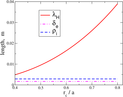
Figure 1: (Color online) Ideal-MHD inertial-layer width $\lambda_{H}$ as a function of $r_{c}$ [with $k_{\|}(r_{c})=0$] compared to the ion thermal gyroradius $\rho_{i}$ (computed for $T_{i}=5$ keV) and to the electron skin depth $\delta_{e}$. Screw pinch geometry with $R_{0}=5$ m, $a=1$ m, $B_{0}=2.5$ T is considered. For these parameters, the fluid inertial length is larger than the kinetic radial scales $\rho_{i}=2.8\times 10^{-3}$ m and $\delta_{e}=1.7\times 10^{-3}$ m.

We consider a sequence of straight-tokamak equilibria corresponding to different locations of the rational flux surface $r_{c}$. In Fig. 1, the ideal-MHD inertial-layer width $\lambda_{H}$ is shown as a function of $r_{c}$. One sees that $\lambda_{H}$ exceeds both the ion gyroradius $\rho_{i}=2.8\times 10^{-3}$ m and the electron skin depth $\delta_{e}=\rho_{e}/\sqrt{\beta_{e}}=1.7\times 10^{-3}$ m for all equilibria considered.

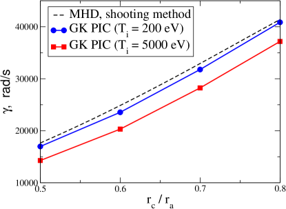
Figure 2: (Color online) Internal kink mode growth rate resulting from the gyrokinetic PIC simulations (at two different ion temperatures) compared to the results of the ideal-MHD eigenvalue calculations (the MHD eigenvalue problem has been numerically solved using the shooting method). The agreement between the ideal MHD and the gyrokinetic simulations is very good, especially at the smaller ion temperature (i. e. at the smaller ion gyroradius). One sees that the gyrokinetic kink mode is somewhat stabilised when the ion gyroradius increases. This FLR effect is absent in the ideal MHD description.

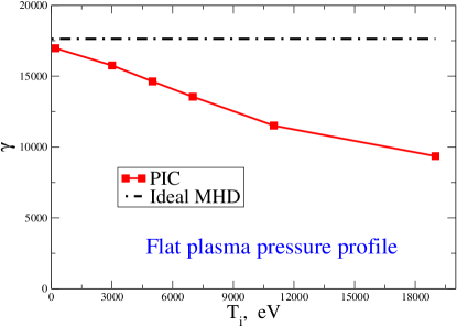
Figure 3: (Color online) Internal kink mode growth rate (resulting from the gyrokinetic PIC simulations) as a function of the plasma temperature ($T_{i}=T_{e}$). The growth rate decreases at larger $T_{i}$ which should be attributed to FLR-stabilization. The rational flux surface is localized at $r_{c}/a=0.5$. For comparison, the ideal-MHD result is shown (which does not depend on the ion temperature).

In Fig. 2, the internal kink mode growth rate resulting from the gyrokinetic PIC simulations is compared to the results of the ideal-MHD eigenvalue calculations [the MHD eigenvalue problem Eq. (19) has been numerically solved using the shooting method]. One sees that the mode is more unstable for larger $r_{c}$, i. e. when a larger plasma column is involved in the instability [this can also be seen formally from Eq. (16)]. The quantitative agreement between the ideal MHD and the gyrokinetic simulations is very good when the ion temperature is small $T_{i}=200$ keV (implying ion gyroradius small). When the ion gyroradius increases, the kink mode becomes less unstable (although the quialitative dependence on $r_{c}$ remains the same). The mode is still an MHD-like internal kink instability but this will change when $k_{\perp}\rho_{i}>1$ with $k_{\perp}\sim 1/\lambda_{H}$ (see Sec. III.2). One can quantify the ion-FLR effects considering a sequence of internal kink modes keeping all the parameters constant except the plasma temperature ($T_{i}=T_{e}$). Note that the ideal-MHD growth rate does not depend on the temperature (for a flat profile such as used in these simulations). In contrast, the gyrokinetic simulations show that the kink mode growth rate decreases with the plasma temperature (see Fig. 3). This FLR-stabilization effect can be quite substantial when the ion temperature is large enough. Note that a similar ion-FLR stabilization has already been observed for other MHD modes (see the gyrokinetic simulations of the Toroidal Alfvén Eigenmodes in Ref. Mishchenko_fast ). The stabilization is caused by the gyro-averaging operation acting on the perturbed electromagnetic field. Clearly, this effect is absent in the ideal MHD description and can be found only with a kinetic treatment.

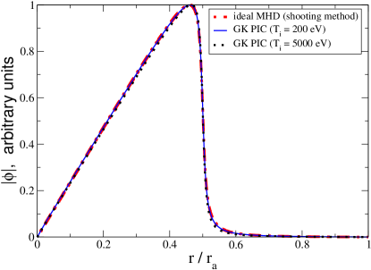
Figure 4: (Color online) Internal kink mode radial structure in the regime with $\lambda_{H}\gg\rho_{i}$. The mode changes abruptly at the rational flux sruface $r_{c}=0.5$ which is a well-known property of the intenal kink modes. One sees a perfect agreement between the eigenmode structures obtained from the initial-value gyrokinetic PIC simulations and solving (numerically) an ideal-MHD eigevalue problem.

In Fig. 4, we compare the ideal-MHD eigenmode structure with the radial pattern found in the gyrokinetic simulations. An excellent agreement is found. The ideal-MHD displacement $\xi\sim\phi/r$ corresponding to Fig. 4 has the well-known top-hat structure. The poloidal fluid velocity $v_{\theta}\sim\partial\phi/\partial r$ is clearly strongly increased at the rational flux surface, as must be the case for the internal kink mode.

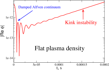
Figure 5: (Color online) Internal kink mode evolution in the regime with $\lambda_{H}\gg\rho_{i}$. The rational flux sruface is located at $r_{c}=0.7$. The plasma temperature $T_{i}=T_{e}=5$ keV. The initial perturbation (a Gaussian) decays in the continuum of the shear Alfvén waves which are reorganized afterwards into the internal kink eigenmode.

In Fig. 5, the internal kink mode evolution is shown (here, the rational flux surface is located at $r_{c}=0.7$; the plasma temperature $T_{i}=T_{e}=5$ keV). One sees how the initial perturbation (which has had a Gaussian shape in the radial direction) decays in the continuum of the shear Alfvén waves and is then re-organized as an unstable internal kink mode. The ion gyroradius must be resolved in order to correctly reproduce the continuum-decay phase of the mode evolution. The frequency of this mode is zero (this is a well-known property of the ideal MHD modes, related to the Hermitian symmetry of the underlying equations; this property can also be reproduced in the gyrokinetic simulations).

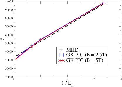
Figure 6: (Color online) Pressure gradient effect on the kink mode in the MHD regime. Equilibria with “large” and “moderate” magnetic fields ($B=5$ T and $B=2.5$ T) have been compared. The plasma temperature $T_{i}=T_{e}=3$ keV. The result does not depend on $B$ (as expected according to MHD theory) and the agreement between the gyrokinetic simulations and the MHD computation is good.

So far, we have considered the current-driven internal kink mode (the plasma pressure was chosen to be flat). Now, let us include the pressure destabilization in our simulations. In Fig. 6, the kink-mode growth rate is plotted as a function of the plasma density gradient. For the density profile, we choose $s_{n}=0.5$, $\Delta_{n}=0.2$ [see Eq. (15)]. The plasma temperature $T_{i}=T_{e}=3$ keV is taken to be flat. The resonant flux surface has been located at $r_{c}=0.7$. Two cases, one with a large magnetic field $B=5$ T and the other with a moderate magnetic field $B=2.5$ T, were considered [keeping $\beta(s_{n})=0.00773$ constant]. One sees from Eq. (18) that the ideal-MHD result does not depend on the magnetic field strength. Indeed, the gyrokinetic simulations reproduce this property. The agreement between the gyrokinetic simulations and the MHD result is good for both values of the ambient magnetic field. The kink-mode growth rate increases with the density (pressure) gradient, as expected.

Summarizing, we have considered the internal kink mode in the regime $\rho_{i}<\lambda_{H}$ (ions in the resonant layer are magnetized). In this regime, the properties of the kink mode agree well with the ideal MHD expectations (thus providing a benchmark for our simulations). The only effect found beyond ideal MHD, is an ion-FLR stabilization of the internal kink mode (which however can be quite substantial).

III.2 Internal kink mode: “FLR regime”

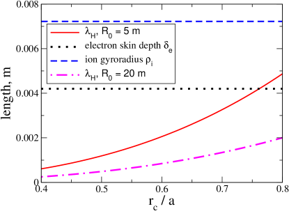
Figure 7: (Color online) Ideal-MHD inertial-layer width compared with the ion thermal gyroradius and the electron skin depth. Screw pinches with $a=0.5$ m, $B_{0}=1$ T, $R_{0}=5$ m and $R_{0}=20$ m are considered. Here, the MHD drive is much smaller compared to the case shown in Fig. 1 (especially when $R_{0}=20$ m). As a consequence, the ion gyroradius is much larger than the MHD inertial length indicating the importance of the FLR effects (and ion sub-Larmor scales) in the mode evolution (kinetic regime of the $m=1$, $n=1$ mode).

We now consider the case when the thermal ion gyroradius exceeds the ideal-MHD inertial width $\rho_{i}\gg\lambda_{H}$. The parameters here are as follows. The straight tokamak has the minor radius $a=0.5$ m, the ambient magnetic field $B_{0}=1$ T, and the plasma density $n_{0}=1.6\times 10^{18}~{}{m^{-3}}$ (it corresponds to $\beta=0.00644$ when $T_{i}=T_{e}=5$ keV). Equilibria with the major radii $R_{0}=5$ m and $R_{0}=20$ m have been considered (changing the major radius one can change the aspect ratio and, consequently, the inertial-layer width $\lambda_{H}$ while $\rho_{i}/r_{a}$ is kept fixed). The comparison between the inertial layer width $\lambda_{H}$, the thermal ion gyroradius $\rho_{i}$, and the electron skin depth $\delta_{e}$ is shown for different aspect ratios in Fig. 7. One sees that the ion gyroradius is indeed much larger than all other relevant scales, especially when $R_{0}=20$ m (this case corresponds to a particularly weak, almost vanishing ideal-MHD drive).

In this regime (ions are demagnetized in the resonant layer), Ref. Porcelli91 predicts the existence of an unstable collisionless $m=1$ tearing mode. In the case $\lambda_{H}\rightarrow 0$, the growth rate of this mode is given by the expression Porcelli91 :

$$\gamma=\frac{\hat{s}_{q}(r_{c})v_{A}(r_{c})}{R_{0}}\;\frac{(\delta_{e}\rho_{i}^{2})^{1/3}}{r_{c}}\ ,\;\;\;v_{A}=\frac{B_{0}^{2}}{\sqrt{\mu_{0}m_{i}n_{0}}}\ ,\;\;\;\hat{s}_{q}=\frac{r}{q}\,{\frac{{\rm{d}}q}{{\rm{d}}r}}.$$ (20)

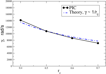
Figure 8: (Color online) Internal kink mode growth rate resulting from the gyrokinetic PIC simulations compared to the analytic prediction for the collisionless $m=1$ tearing mode Porcelli91 $\gamma\sim(\delta_{e}\rho_{i}^{2})^{1/3}/r_{c}$. Here, the parameters chosen are $T_{i}=T_{e}=11$ keV and $R_{0}=20$ m. One sees a very good agreement between the theory and simulations.

In Fig. 8, we plot the growth rate resulting from the gyrokinetic PIC simulations (corresponding to the pinch with $R_{0}=20$ m, i. e. very small $\lambda_{H}$) compared to the analytic prediction for the collisionless $m=1$ tearing mode as a function of the resonant layer position. In contrast to the “ideal-MHD” regime (see Fig. 2), the mode is more unstable for smaller $r_{c}$, indicating a change in the underlying physical mechanism: reconnection (electron physics) in addition to the poloidal plasma rotation (ions). The agreement between the gyrokinetic result and the theoretical prediction Eq. (20) is very good.

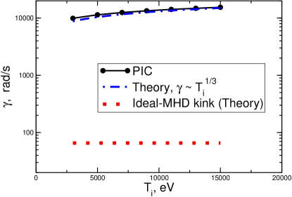
Figure 9: (Color online) Internal kink mode growth rate (resulting from the gyrokinetic PIC simulations for $R_{0}=20$ m) as a function of the plasma temperature ($T_{i}=T_{e}$). The growth rate increases with the temperature contrary to the ideal-MHD case (see Fig. 3). The rational flux surface is localized at $r_{c}=0.4$. The agreement of the simulations with the theory is very good. For reference, the ideal-MHD growth rate corresponding to the parameters chosen is plotted. One sees that the growth rate of the kinetic-kink (reconnecting) mode is more than two orders of magnitude larger than the growth rate of the marginally-unstable ideal-MHD mode.

In Fig. 9, we consider the dependence of the kink-mode growth rate on the ion temperature (ion-FLR effect). One sees that in the regime of demagnetized ions (inside the resonant layer), the mode is further destabilized when the ion gyroradius increases. This FLR-destabilization is in contrast to the MHD-type internal kink mode considered previously, which was FLR-stabilized (see Fig. 3). The numerical result has been compared with the analytical expression Eq. (20). The agreement is again very good. For comparison, we plot the growth rate predicted by the ideal MHD theory, which is more than two orders of magnitude smaller. It indicates that the kinetic effects can dominate the kink mode physics, certainly around ideal marginal stability.

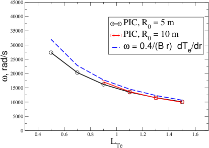
Figure 10: (Color online) Frequency of the kinetic internal kink mode (collisionless $m=1$ tearing mode) as a function of the electron temperature gradient. Ion temperature and density are kept constant. For comparison, an estimate for the drift-tearing mode frequency $\omega=0.4\,\omega_{{\rm T}e}$ Cowley86 is plotted. One sees that the agreement is good. The mode properties for two different aspect ratios (and, consequently, $\lambda_{H}$) are compared (major radius is varied whereas the minor radius is kept fixed). One sees that the mode frequency does not depend on $\lambda_{H}$ and, hence, is set exclusively by the diamagnetic frequency associated with the electron temperature gradient.

Finally, we consider the effect of the electron temperature gradient on the collisionless $m=1$ tearing mode. We employ a temperature profile with $s_{{\rm T}}=r_{c}/r_{a}=0.5$ (the position of the maximal gradient coincides with that of the resonant flux surface) and $\Delta_{s}=0.2$ [see Eq. (15)]. The ion temperature and the plasma density are taken to be flat. As a consequence of the diamagnetic effect associated with the finite electron temperature gradient, the mode acquires a finite frequency and becomes a drift-tearing instability (see e. g. Cowley86 ; Zocco2012 ). The frequency resulting from the gyrokinetic PIC simulations is plotted in Fig. 10 as a function of $L_{Te}$ (electron temperature gradient length) for two different values of the major radius: $R_{0}=5$ m and $R_{0}=10$ m (recall that the ideal-MHD drive and, consequently, $\lambda_{H}$ decrease with the aspect ratio). One sees that the frequency is the same for both values of $R_{0}$. Hence, it is set exclusively by the diamagnetic frequency at the position of the resonant flux surface $\omega_{{\rm T}e}=1/(Br_{c})\,{\rm{d}}T_{e}/{\rm{d}}r$. In fact, the frequency of the collisionless $m=1$ drift-tearing mode appears to satisfy $\omega\approx 0.4\,\omega_{{\rm T}e}$ (cf. Ref. Cowley86 ).

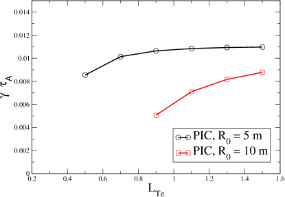
Figure 11: (Color online) Growth rate of the kinetic internal kink mode (collisionless $m=1$ tearing mode) as a function of the electron temperature gradient (same parameters as in Fig. 10). In contrast to the frequency, the growth rate is much smaller at larger $R_{0}$ (note the normalization to $\tau_{A}\propto 1/R_{0}$.) In this case, the continuum damping (set by the mode frequency which is equal for both values of $R_{0}$) corresponds to a larger fraction of the smaller growth rate, making the stabilization mechanism more effective.

The growth rate as a function of $L_{Te}$ (electron temperature gradient length) is plotted in Fig. 11. As expected Cowley86 ; Zocco2012 , the electron temperature gradient stabilizes the collisionless drift-tearing $m=1$ mode. Physically, it has been shown in Ref. Zocco2012 that the drift-tearing mode can couple to a stable Kinetic Alfvén Wave (KAW) which leads to a stabilization of the mode. Another way to explain this stabilization effect has been elaborated in Ref. Breizman_fishbones (in the fishbone context). In short, the finite-frequency mode can interact with the Alfvén continuum (or, alternatively, with the KAWs as in Zocco2012 ) and thus undergo continuum damping (as is well-known from the context of Toroidal Alfvén Eigenmodes Zonca_Chen_92 ; Berk_conti_92 ; Rosenbluth_conti_92 ). Of course, the frequency of the drift-tearing $m=1$ mode is quite small, so that the continuum damping acts only very close to the resonant flux surface (the surface of vanishing $k_{\|}$) where the condition $\omega^{2}=k_{\|}^{2}(r_{A})v_{A}^{2}(r_{A})$ can be satisfied. The frequency of the $m=1$ drift-tearing mode increases with the electron temperature gradient which makes the continuum damping more efficient at smaller $L_{Te}$ – to the point of a complete stabilization. Note that in Fig. 11 the stabilization appears to be stronger for the case with the larger major radius $R_{0}=10$ m. In this case, the absolute value of the growth rate would be smaller compared with the configuration with $R_{0}=5$ m, even for the flat temperature profiles, because the growth rate inversely scales with the Alfvén time $\tau_{A}\sim R_{0}$. Thus, the continuum damping, which is determined by the mode frequency (set by the electron temperature gradient and thus equal for both values of $R_{0}$), corresponds to a larger fraction of the smaller growth rate when $R_{0}=10$ m.

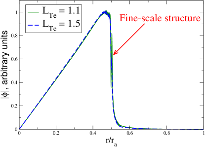
Figure 12: (Color online) Kinetic-kink eigenmode ($R_{0}=10$ m) compared at different electron temperature gradient lengths $L_{{\rm T}e}$. A fine-scale structure develops around the rational flux surface [indicating the continuum damping at the position of the resonance $\omega=\pm k_{\|}(r_{A})v_{A}$, see Fig. 13 for details]. The fine-scale structure is more pronounced (see Fig. 13) at larger electron temperature gradients (where the mode frequency is larger and, consequently, the continuum damping is stronger).

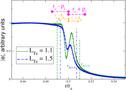
Figure 13: (Color online) The eigenmodes from Fig. 12 zoomed around the rational flux surface. For comparison, the ion gyroradius and electron skin depth scales are plotted. Also, the positions of the shear Alfvén resonances are indicated (the kinetic Alfvén wave resonances would be more precise). One sees that the relevant radial scales are smaller than the ion gyroradius. Kinetic Alfvén waves are excited at the resonant positions causing a stabilization of the collisionless $m=1$ drift-tearing mode (through the “continuum” damping mechanism).

In Fig. 12, the radial mode structure is shown. One sees that in addition to the conventional internal kink eigenmode, a complicated fine-scale structure appears at the resonant flux surface. This structure is caused by the continuum damping of the instability. One can see that it becomes more pronounced when the electron temperature gradient increases (see Fig. 13). We can estimate the position of the shear Alfvén resonances using the expression:

$$r_{A}=r_{c}\pm\frac{\omega\tau_{A}}{q^{\prime}(r_{c})}\ ,\;\;\;\tau_{A}=R_{0}/v_{A}$$ (21)

For the safety factor profile chosen, $q^{\prime}(r_{c})=0.8$. Fig. 13 indicates that the fine-scale structure developed could be understood as Kinetic Alfvén Waves (recall that we use a non-local expression for the polarization density) resonantly excited by the collisionless $m=1$ tearing mode in the positions approximately satisfying the shear Alfvén wave resonance condition $\omega^{2}\approx k_{\|}^{2}(r_{A})v_{A}^{2}(r_{A})$ (the Kinetic Alfvén Wave resonance would be more precise). The drift-tearing (kinetic-kink) mode is damped because of its coupling to the Kinetic Alfvén Waves (a “continuum”) at the resonant positions. A finite frequency of the tearing mode is required for this process to function. This frequency is provided by the diamagnetic effect due to a finite electron-temperature gradient.

IV Conclusion

In this paper we have studied the internal kink modes in a straight-tokamak geometry using the global gyrokinetic particle-in-cell code GYGLES. Both electron and ion gyrocenters were treated kinetically, but collisions were ignored. The simulations have shown that the kink mode properties depend strongly on the ratio between the ideal-MHD inertial-layer scale and the gyroradius. In the “MHD regime”, the kink mode becomes more unstable if the rational flux surface “moves” (during the parameter scan) outwards. In the “FLR regime”, however, the kinetic-kink mode (the “collisionless $m=1$ tearing mode” Porcelli91 ) is more unstable for resonant magnetic surfaces located closer to the magnetic axis ($1/r_{c}$ dependence of the growth rate). Similarly, the scaling with respect to the ion temperature is also opposite: the FLR-stabilization for the MHD-type kink mode has been observed whereas the “collisionless $m=1$ tearing mode” is FLR-destabilized. One could speculate Porcelli91 that the most unstable $m=1,n=1$ instabilities observed in real hot plasmas often correspond to the “collisionless $m=1$ tearing” (kinetic-kink) modes rather than the classical ideal-MHD internal kink modes since usually the real plasmas are at the marginal MHD-kink stability boundary so that the ion gyroradius can easily overcome the ideal inertial length (thus bringing the instability into the kinetic regime). The kinetic-kink modes, however, can be sensitive to the shape of plasma profiles and can be stabilized e. g. by the electron temperature gradient (through a combination of the diamagnetic and continuum-damping effects).

Looking forward, gyrokinetic simulations of the internal kink modes in tokamak geometry would be of interest. In these simulations, the effects of the guiding center orbits in the resonant region, the kinetic trapped-ion and fast-particle (e. g. fishbone) effects in the ideal region should be addressed. Also, gyrokinetic simulations of interchange instabilities (both in straight and toroidal geometries) could be performed in the future.

ACKNOWLEDGMENTS

We acknowledge P. Helander and A.  Schekochihin who have supported this work. R. Kleiber’s help on the shooting algorithm is appreciated. We thank J. Connor for carefully reading this manuscript. The simulations have been performed on the HPC-FF supercomputer (Jülich, Germany) and the HELIOS supercomputer (Aomori, Japan) as well as on the local cluster in Greifswald (H. Leyh’s help is appreciated). Joint work on this paper has been enabled by the Gyrokinetic Meetings in Vienna and Madrid. We thank N. Mauser (Wolfgang Pauli Institute, Vienna) and I. Calvo (CIEMAT, Madrid) for organizing these workshops. Support by the Leverhulme Trust International Academic Network in Magnetised Plasma Turbulence and Euratom Mobility is also appreciated.

References

- (1) W. A. Newcomb, Annals of Physics 10, 232 (1960).
- (2) V. D. Shafranov, Zh. Tekh. Fiz. 40, 241 (1970).
- (3) M. N. Rosenbluth, R. Y. Dagazian, and P. H. Rutherford, Phys. Fluids 16, 1894 (1973).
- (4) M. N. Bussac, R. Pellat, D. Edery, and J. L. Soule, Phys. Rev. Lett. 35, 1638 (1975).
- (5) S. von Goeler, W. Stodiek, and N. Sauthoff, Phys. Rev. Lett. 20, 1201 (1974).
- (6) K. McGuire, R. Goldston, M. Bell, M. Bitter, K. Bol, K. Brau, D. Buchenauer, T. Crowley, S. Davis, F. Dylla, H. Eubank, H. Fishman, R. Fonck, B. Grek, R. Grimm, R. Hawryluk, H. Hsuan, R. Hulse, R. Izzo, R. Kaita, S. Kaye, H. Kugel, D. Johnson, J. Manickam, D. Manos, D. Mansfield, E. Mazzucato, R. McCann, D. McCune, D. Monticello, R. Motley, D. Mueller, K. Oasa, M. Okabayashi, K. Owens, W. Park, M. Reusch, N. Sauthoff, G. Schmidt, S. Sesnic, J. Strachan, C. Surko, R. Slusher, H. Takahashi, F. Tenney, P. Thomas, H. Towner, J. Valley, R. White, Phys. Rev. Lett. 50, 891 (1983).
- (7) B. B. Kadomtsev, Sov. J. Plasma Phys. 1, 389 (1975).
- (8) G. Ara et al., Annals of Physics 112, 443 (1977).
- (9) J. F. Drake, Phys. Fluids 21, 1777 (1978).
- (10) B. Basu and B. Coppi, Phys. Fluids 24, 465 (1980).
- (11) T. M. Antonsen and B. Coppi, Phys. Lett. A 81, 335 (1981).
- (12) S. C. Cowley, R. M. Kulsrud, and T. S. Hahm, Phys. Fluids 29, 3230 (1986).
- (13) F. Pegoraro, F. Porcelli, and T. J. Schep, Phys. Fluids B 1, 364 (1989).
- (14) F. Porcelli, Phys. Rev. Lett. 66, 425 (1991).
- (15) F. Porcelli, D. Boucher, and M. N. Rosenbluth, Plasma Phys. Controlled Fusion 38, 2163 (1996).
- (16) J. W. Connor, R. J. Hastie, and A. Zocco, Plasma Phys. Controlled Fusion 54, 035003 (2012).
- (17) A. Martynov, J. P. Graves, and O. Sauter, Plasma Phys. Controlled Fusion 47, 1743 (2005).
- (18) F. D. Halpern, D. Leblond, H. Lütjens, and J-F. Luciani, Plasma Phys. Controlled Fusion 53, 015011 (2011).
- (19) F. D. Halpern, H. Lütjens, and J-F. Luciani, Phys. Plasmas 18, 102501 (2011).
- (20) T. S. Hahm, W. W. Lee, and A. J. Brizard, Phys. Fluids 31, 1940 (1988).
- (21) W. W. Lee, J. Comp. Phys. 72, 243 (1987).
- (22) H. Naitou, K. Tsuda, W. W. Lee, and R. D. Sydora, Phys. Plasmas 2, 4257 (1995).
- (23) H. Naitou, K. Kobayashi, H. Hashimoto, S. Tokuda, and M. Yagi, J. Plasma Fusion Res. Series 8, 1158 (2009).
- (24) H. Qin, W. M. Tang, W. W. Lee, and G. Rewoldt, Phys. Plasmas 6, 1575 (1999).
- (25) P. Lauber, Ph.D. thesis, Technische Universität München, 2003.
- (26) A. Mishchenko, R. Hatzky, and A. Könies, Phys. Plasmas 15, 112106 (2008).
- (27) A. Mishchenko, A. Könies, and R. Hatzky, Phys. Plasmas 16, 082105 (2009).
- (28) A. Mishchenko, A. Könies, and R. Hatzky, Phys. Plasmas 18, 012504 (2011).
- (29) M. Fivaz, S. Brunner, G. de Ridder, O. Sauter, T. M. Tran, J. Vaclavik, L. Villard, and K. Appert, Comp. Phys. Commun. 111, 27 (1998).
- (30) A. Mishchenko, A. Könies, and R. Hatzky, Phys. Plasmas 12, 062305 (2005).
- (31) A. J. Brizard and T. S. Hahm, Reviews of Modern Physics 79, 421 (2007).
- (32) C. de Boor, A Practical Guide to Splines (Springer-Verlag, New York, 1978).
- (33) K. Höllig, Finite Element Methods with B-Splines (Society for Industrial and Applied Mathematics, Philadelphia, 2003).
- (34) A. Mishchenko, R. Hatzky, and A. Könies, Phys. Plasmas 11, 5480 (2004).
- (35) A. Mishchenko, A. Könies, and R. Hatzky, in Proc. of the Joint Varenna-Lausanne International Workshop (Società Italiana di Fisica, Bologna, 2004).
- (36) R. Hatzky, A. Könies, and A. Mishchenko, J. Comp. Phys. 225, 568 (2007).
- (37) A. Ödblom, B. N. Breizman, S. E. Sharapov, T. C. Hender, and V. P. Pastukhov, Phys. Plasmas 9, 155 (2002).
- (38) F. Zonca and L. Chen, Phys. Rev. Lett. 68, 592 (1992).
- (39) H. L. Berk, J. W. Van Dam, Z. Guo, and D. M. Lindberg, Phys. Fluids B 4, 1806 (1992).
- (40) M. N. Rosenbluth, H. L. Berk, J. W. Van Dam, and D. M. Lindberg, Phys. Fluids B 4, 2189 (1992).