Role of conviction in nonequilibrium models of opinion formation

Abstract

We analyze the critical behavior of a class of discrete opinion models in the presence of disorder. Within this class, each agent opinion takes a discrete value ($\pm 1$ or 0) and its time evolution is ruled by two terms, one representing agent-agent interactions and the other the degree of conviction or persuasion (a self-interaction). The mean-field limit, where each agent can interact evenly with any other, is considered. Disorder is introduced in the strength of both interactions, with either quenched or annealed random variables. With probability $p$ (1-$p$), a pairwise interaction reflects a negative (positive) coupling, while the degree of conviction also follows a binary probability distribution (two different discrete probability distributions are considered). Numerical simulations show that a non-equilibrium continuous phase transition, from a disordered state to a state with a prevailing opinion, occurs at a critical point $p_{c}$ that depends on the distribution of the convictions, the transition being spoiled in some cases. We also show how the critical line, for each model, is affected by the update scheme (either parallel or sequential) as well as by the kind of disorder (either quenched or annealed).

I Introduction

In the last decades, diverse questions of social dynamics have been studied through statistical physics techniques. In fact, simple models allow to simulate and understand real problems such as elections, spread of information, vehicle traffic or pedestrian evacuation, amongst many others loreto_rmp . As a feedback, these issues are attractive to physicists because of the occurrence of order-disorder transitions, scaling and universality, among other typical features of physical systems.

Concerning the particular subject of opinion dynamics, several models have been proposed in order to study the emergence of consensus (for a recent review, see loreto_rmp ). As concrete examples, let us mention opinion models based on outflow dynamics sznajd ; sznajd_meu ; sznajd_meu_pmco , majority rules redner ; galam_maj ; galam ; galam_epjb and bounded confidence deffuant , as well as kinetic exchange lccc ; biswas ; p_sen ; biswas11 . Recently, the effects of negative interactions biswas ; wang and network dynamics newman ; kozma ; gross_review in opinion formation have also been considered.

In this work we introduce heterogeneity in the degree of persuasion or conviction of the agents. It is mimicked by a parameter which gauges the tendency of an agent to hold its opinion or (if negative) change mind spontaneously. Then, we study the impact of persuasion in the critical behavior of a non-equilibrium model of opinion formation with a finite fraction of random negative agent-agent interactions. We study two classes of disorder (either quenched or annealed) both for the strength of convictions and for agent-agent couplings. We also consider two different kinds of update, either sequential or parallel. Numerical Monte Carlo simulations show that a continuous order-disorder phase transition, where order is characterized by a dominating opinion, can occur in all the variants of the model considered. However, the critical line is strongly affected by the distribution of convictions. Moreover, it is also affected both by the update scheme and by the nature of the random variables, as occurs in other models stauffer ; sabatelli ; adriano_updates ; bolle ; schonfisch ; caron .

This work is organized as follows. In Section II we present the opinion model and define its microscopic rules. Numerical results are discussed in Section III in connection with the analytical considerations presented in the Appendix. Section IV contains the conclusions and final remarks.

II The model

We consider an opinion model based on kinetic exchange lccc ; biswas ; p_sen ; biswas11 . At a given time step $t$, each agent $i$ has a discrete opinion $o_{i}(t)=-1,0$ or $1$, that evolves according to

$$o_{i}(t+1) = C_{i}\,o_{i}(t)+\mu_{ij}\,o_{j}(t)~{},$$

$$o_{j}(t+1) = C_{j}\,o_{j}(t)+\mu_{ji}\,o_{i}(t)~{},$$ (1)

where $C_{i}$ is the conviction of agent $i$ and $\mu_{ij}$ is the strength of the influence it suffers from a randomly chosen agent $j$ in a fully-connected graph. If the value of the opinion exceeds (falls below) the value 1 ($-1$), then it adopts the extreme value 1 ($-1$). Pairwise interaction strengths are random variables distributed according to the binary probability density function (PDF)

$$F(\mu_{ij})=p\,\delta(\mu_{ij}+1)+(1-p)\,\delta(\mu_{ij}-1)~{}.$$ (2)

In other words, the agents can exchange opinions with positive ($+1$) or negative ($-1$) influences, and $p$ quantifies the mean fraction of negative ones biswas . In magnetic systems, analogous positive (negative) interactions would correspond to ferro (anti-ferro) couplings. Notice certain similarities with what is known as the (mean-field) Blume-Capel model blume_capel : each opinion has three different states (spin-1 Ising); agents interact through ferromagnetic/anti-ferromagnetic couplings; in the Hamiltonian defining the model, there are quadratic terms representing the interaction of the spins with the crystal field and that can be related to the agents self-interaction; finally, the Blume-Capel model may include the interaction with an external field, that, although neglected here, may be opportune in opinion models as well, representing for instance propaganda or other external conditioning feature nuno_physicaA . Since in the present model, couplings are random: positive/ferromagnetic (or negative/anti-ferromagnetic) with probability $1-p$ (or $p$), it remits to the random-bond version of the Blume-Capel model, with random local competing fields. Moreover, here there is absence of thermal fluctuations, corresponding to the zero temperature limit of thermal spin models. Zero temperature random Ising-like models, for instance containing either local or global random fields, have already been considered to model group decision making decision ; collective . Notice however that differently from those magnetic models, the interactions occur by pairs and there is not an energy-like function to optimize. As a consequence of the different dynamical rules, the critical behavior is not related to that of usual equilibrium models, as we will see in the results presented in the next Section. For instance, no frozen or spin-glass phase is observed. The phenomenological differences were explained before as being due to the lack of frustration, despite the competitive random interactions, as soon as interactions do not occur simultaneously biswas .

The influence of an individual over another one needs not be reciprocal (i.e., not necessarily $\mu_{ij}=\mu_{ji}$), however, whether interactions are symmetric or not, does not affect the results. If $C_{i}=1$ for all $i$ (i.e., $q=1$), one recovers the model of Ref. biswas , for which there is an order-disorder transition at a critical value $p_{c}=1/4$. As discussed in Ref. biswas , the effect of negative interactions is similar to that produced by Galam’s contrarians in opinion models galam_cont . We will discuss this relation in more details in the following.

However, more realistically, the degree of conviction needs not be unitary nor homogeneous biswas11 . Then we considered two discrete alternatives for the PDFs of the convictions $C_{i}$, namely,

$$G_{1}(C_{i}) = q\,\delta(C_{i}-1)+(1-q)\,\delta(C_{i}-0)\,,$$ (3)

$$G_{2}(C_{i}) = q\,\delta(C_{i}-1)+(1-q)\,\delta(C_{i}+1)\,.$$ (4)

They model the cases where a mean fraction $1-q$ of the individuals have either no convictions or completely change mind, respectively. In comparison to magnetic models, $G_{1}$ and $G_{2}$ are related to random diluted field and random antiferromagnetic impurities, respectively spin1BC .

In both cases, the model of Ref. biswas is recovered for $q=1$. Notice that, differently from the Sznajd dynamics sznajd , where each agent interacts with a group of individuals at a time, in the present exchange model, interactions are pairwise.

We will show how the heterogeneity of convictions favors disorder or even provokes the destruction of the order-disorder phase transition. Moreover, we will analyze two distinct kinds of the random variables $C_{i}$ and $\mu_{ij}$: they can be either quenched or annealed. The former are drawn from the PDFs given by Eqs. (2) and (3) [or (2) and (4)] at the beginning of each simulation and remain fixed during the evolution of the system, whereas the later are renewed at each Monte Carlo step (MCs), where one MCs corresponds to $N$ iterations of Eq. (1), being $N$ the population size.

In addition, we have studied two kinds of upgrades: synchronous (parallel) and asynchronous (random sequential). In the former case, we randomly choose $N$ pairs of agents that interact by means of Eq. (1). Only after the $N$ interactions took place, the states of the $N$ agents are simultaneously renewed, increasing time by one MCs. In the asynchronous case, also $N$ pairs of agents that interact by means of Eq. (1) are randomly chosen at each MCs, but the opinions are assigned a new value at each interaction. A more realistic dynamics probably proceeds in between both schemes.

All simulations start with a random initial distribution of opinions, and all interacting pairs of agents are randomly chosen among the $N$ individuals in the population (which corresponds to a mean-field approach).

III Results

We analyze the critical behavior of the system, in analogy to Ising spin systems, by computing the order parameter

$$O=\left\langle\frac{1}{N}\left|\sum_{i=1}^{N}o_{i}\right|\right\rangle~{},$$ (5)

where $\langle\,...\,\rangle$ denotes disorder or configurational average. Notice that $O$ plays the role of the “magnetization per spin” in magnetic systems. In addition, we also consider the fluctuations $\chi$ of the order parameter (or “susceptibility”)

$$\chi=N\,(\langle O^{2}\rangle-\langle O\rangle^{2})$$ (6)

and the Binder cumulant $U$, defined as

$$U=1-\frac{\langle O^{4}\rangle}{3\,\langle O^{2}\rangle^{2}}\,.$$ (7)

In the following subsections, we will analyze separately the distributions given by Eqs. (3) and (4).

III.1 Model with distribution $G_{1}$

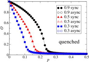
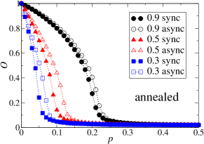
Figure 1: (Color online) Order parameter versus $p$ for quenched (top) and annealed (bottom) random variables of Eq. (3), with typical values of $q$ indicated on the figure. The full (open) symbols are results of simulations with synchronous (asynchronous) update. The population size is $N=1000$ and data are averaged over $100$ realizations.

For the distribution $G_{1}(C_{i})$ of Eq. (3), the mean fraction of null convictions is $1-q$. Such agents with no convictions evolve influenced only by the interaction with other randomly chosen agents.

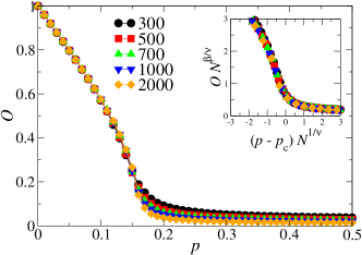
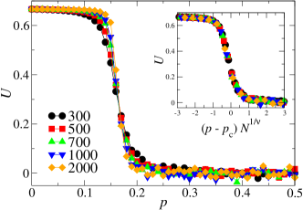
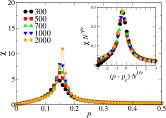
Figure 2: (Color online) Order parameter, Binder cumulant and susceptibility for the PDF of Eq. (3) with $q=0.5$ and different population sizes $N$ indicated on the figure (main plots). The corresponding scaling plots are shown in the respective insets. Data are for quenched random variables and synchronous update scheme. The best data collapse was obtained for $p_{c}\sim 0.167$, $\beta\sim 0.5$, $\gamma\sim 1.0$ and $1/\nu\sim 0.5$.

In Fig. 1 we exhibit results for the order parameter as a function of $p$ for typical values of $q$, allowing to compare the cases with quenched (top) and annealed (bottom) disorder. One can see that the curves for synchronous and asynchronous updates in the quenched case are almost identical, indicating that the critical behavior is not modified by the update scheme when we consider frozen disorder. On the other hand, if we allow the disorder to fluctuate in time, the results for synchronous and asynchronous updates are different.

We have verified numerically that, in all the analyzed cases of disorder and update scheme, the system undergoes a non-equilibrium phase transition for all values of $q>0$. The transition separates an ordered phase, where one of the extreme opinions ($+1$ or $-1$) dominates, from a disordered one, where the three opinions coexist equally. A condition that was also obtained analytically for the synchronous annealed case (see the Appendix).

In order to locate the critical points $p_{c}(q)$ numerically, we have performed simulations for different population sizes $N$. Thus, the transition points $p_{c}(q)$ are estimated, for each value of $q$, from the crossing of the Binder cumulant curves for the different sizes. In addition, a finite-size scaling analysis was performed, in order to obtain an estimate of the critical exponents $\beta$, $\gamma$ and $\nu$. As an illustration, we exhibit in Fig. 2 the behavior of the quantities of interest as well as the scaling plots for $q=0.5$, quenched random couplings and synchronous updates. Our estimates for the critical exponents coincide with those for the original model ($q=1$), i.e., we obtained $\beta\sim 0.5$, $\gamma\sim 1.0$ and $1/\nu\sim 0.5$. These exponents are robust: they are the same for all values of $q$, independently of the update scheme considered and of the kind of random variables (quenched or annealed).

Taking into account the critical values $p_{c}(q)$ obtained from the simulations, we exhibit in Fig. 3 the phase diagram of the model in the plane $p$ versus $q$. As discussed before, in the case of quenched variables the frontier is independent of the update scheme. On the other hand, for annealed variables the results are different. This is possibly due to the time fluctuation of the annealed variables, which does not occur in the quenched case. The analytical prediction for the synchronous annealed case is presented in the Appendix.

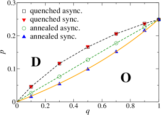
Figure 3: (Color online) Phase diagram of the model defined by Eqs. (1), (2) and (3) in the plane $p$ versus $q$, separating the ordered (O) and disordered (D) phases. The symbols are the finite-size estimates of the critical points $p_{c}(q)$ obtained from the simulations, dashed lines are guides to the eye and the full line is the analytical result predicted by Eq. (9).

III.2 Model with distribution $G_{2}$

For the distribution $G_{2}(C_{i})$ of Eq. (4), a fraction $1-q$ of the convictions $C_{i}$ are $-1$ (instead of being null as in Sec. III.A). Now, some agents $i$ present negative convictions that contribute to a spontaneous change in their opinions, together with the influence of a randomly chosen agent $j$.

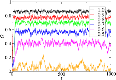
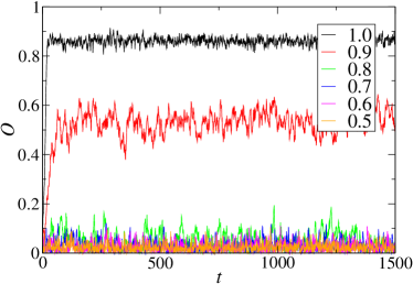
Figure 4: (Color online) Time evolution of the order parameter for $N=1000$, $p=0.1$ and typical values of $q$, labeling the curves from top to bottom. The curves are for: quenched asynchronous (top) and annealed synchronous (bottom). We can observe that a disordered state is reached when the value of $q$ is decreased below a threshold.

Differently from the case where the PDF of convictions is given by Eq. (3), analyzed in Sec. III.A, now we can observe that there is a threshold $q_{c}$ below which the system is always in a disordered state, for all values of $p$.

The time evolution of the order parameter is illustrated in Fig. 4 for the quenched asynchronous and annealed synchronous cases. Similar evolution is observed for the other two combinations too. For sufficiently low $q$, none of the two extreme opinions dominates. Moreover, we verified that in such cases the fraction of each one of the three possible opinions is again $1/3$ in average, indicating complete disorder. This result was also found theoretically for the annealed synchronous case (see Appendix).

In the cases where a transition occurs, a finite-size scaling analysis was perfomed as in Sec. III.A. The same mean-field exponents were obtained, independently of the update scheme considered and of the kind of random variables. The phase diagram for the different types of update and random variables is shown in Fig. 5. The analytical prediction for the synchronous annealed case, derived in the Appendix, is also included. In such case, Eq. (10) predicts that for $q<3/4$ no transition occurs, and the system is always in a disordered state.

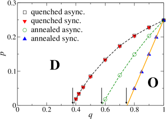
Figure 5: (Color online) Phase diagram of the model defined by Eqs. (1), (2) and (4) in the plane $p$ versus $q$, separating the ordered (O) and disordered (D) phases. The symbols are the finite-size estimates of the critical points $p_{c}(q)$ obtained from the simulations, the dashed lines are guides to the eye, and the full line is the analytical result given by Eq. (10). Notice that the transition is destroyed for values of $q$ below a threshold, indicated schematically by arrows.

IV Final Remarks

In this work we have studied opinion dynamics through a model where agents interact by pairs in a fully-connected graph. The opinions have three different states (spin-1) and the agents interact through random couplings that can be positive/ferromagnetic (or negative/anti-ferromagnetic) with probability $1-p$ (or $p$). Differently from other related models, where the ordered state is marked by consensus, the ordered state is characterized by the upraise of a dominating extreme opinion, which becomes consensual only in the limit in which interactions are all positive ($p=0$). Moreover, there is also a self-interaction term, the conviction, which we considered to assume random values, according to the PDFs $G_{1}$ or $G_{2}$, given by Eqs. (3) and (4), respectively. Then, we aimed to study the impact of the heterogeneity of convictions on the critical behavior of opinion formation. Although states and couplings can take only a few values, a wider spectrum of possibilities is expected to be somehow mapped on the present simpler case.

First, we have considered the PDF $G_{1}$ that aims to model populations where there is a fraction $1-q$ of agents without self-convictions about their opinions, and thus they can be easily persuaded to change their opinions. Our results show that the critical fraction of negative interactions $p_{c}$ below which the population reaches partial agreement decreases smoothly for decreasing values of $q$, collapsing with $p_{c}=0$ only at $q=0$. This order-disorder transition is continuous and the critical exponents are universal and mean-field like, presenting the values $\beta=0.5$, $\gamma=1.0$ and $1/\nu=0.5$ for all values of $q$.

We have also considered the PDF $G_{2}$ for the convictions in societies where some agents have a tendency to change spontaneously their opinions. In this case, disordered states are favored, and the order-disorder boundary falls off rapidly to $p_{c}=0$ for decreasing values of $q$. Thus, in opposition to the previous case, there are threshold values of $q$ below which the system is always in the disordered state. Despite this difference, the order-disorder transition is also continuous and the critical exponents are universal and mean-field like, as in the previous case.

Notice that the introduction of negative interactions, pondered by the probability $p$, produces a similar effect of the so-called Galam’s contrarians galam_cont ; delalama . In fact, in the absence of negative couplings ($p=0$) the system presents consensus states with one of the extreme opinions ($+1$ or $-1$) dominating the population. On the other hand, the inclusion of a fraction of negative interactions leads the system to a disordered state with the coexistence of the three possible opinions $+1$, $-1$ and $0$, analogous to the stalemate state produced by the introduction of contrarians in opinion models, where the two possible opinions, namely $+1$ and $-1$, coexist galam_cont ; delalama . Observe also that the introduction of the conviction parameter $q$ makes this effect more pronounced. In fact, the critical values $p_{c}$ decrease for increasing values of $q$, and in the case of the bimodal distribution $G_{2}$, the effect of the convictions is so strong that it destroys the order-disorder transition.

It is important to notice that the results depend quantitatively (but no qualitatively) on the kind of update scheme used (synchronous or asynchronous) and on the nature (quenched or annealed) of the random variables considered, for the two studied PDFs.

Appendix A

Following the lines of Ref. biswas , we computed critical values for the synchronous annealed case. We first obtained the matrix of transition probabilities whose elements $m_{i,j}$ furnish the probability that a state suffers the shift or change $i\to j$. Let us also define $f_{1}$, $f_{0}$ and $f_{-1}$, the stationary probabilities of each possible state.

In the steady state, the fluxes into and out from a given state must balance. In particular, for the null state, one has $m_{1,0}+m_{-1,0}=m_{0,1}+m_{0,-1}$. Moreover, when the order parameter vanishes, it must be $f_{1}=f_{-1}$. In both cases considered below for the distribution of convictions, those two equalities imply $f_{1}=f_{-1}=f_{0}=1/3$ (disorder condition). This holds in particular at the critical point.

Finally, let us define $r(k)$, with $-2\leq k\leq 2$, the probability that the state shift per unit time is $k$, that is, $r(k)=\sum_{i}m_{i,i+k}$. In the steady, the average shift must vanish, namely,

$$2[r(2)-r(-2)]+r(1)-r(-1)=0\,.$$ (8)

A.1 PDF $G_{1}$

The elements of the transition matrix are

$$m_{1,1} = f_{1}^{2}(1-p)+f_{1}f_{0}q+f_{1}f_{-1}p$$

$$m_{1,0} = f_{1}^{2}qp+f_{1}f_{0}(1-q)+f_{1}f_{-1}q(1-p)$$

$$m_{1,-1} = f_{1}^{2}(1-q)p+f_{-1}f_{1}(1-q)(1-p)$$

$$m_{0,1} = f_{0}f_{1}(1-p)+f_{0}f_{-1}p$$

$$m_{0,0} = f_{0}^{2}$$

$$m_{0,-1} = f_{0}f_{1}p+f_{0}f_{-1}(1-p)$$

$$m_{-1,1} = f_{1}f_{-1}(1-q)(1-p)+f_{-1}^{2}p(1-q)$$

$$m_{-1,0} = f_{1}f_{-1}q(1-p)+f_{0}f_{-1}(1-q)+f_{-1}^{2}qp$$

$$m_{-1,-1} = f_{1}f_{-1}p+f_{0}f_{-1}q+f_{-1}^{2}(1-p)\,.$$

The null average shift condition (8), together with the disorder condition, leads to

$$p_{c}=\frac{q}{2(3-q)}\,.$$ (9)

A.2 PDF $G_{2}$

For this PDF, the transition matrix is

$$m_{1,1} = f_{1}^{2}q(1-p)+f_{1}f_{0}q+f_{1}f_{-1}qp$$

$$m_{1,0} = f_{1}^{2}(qp+(1-q)(1-p))+f_{1}f_{-1}(p+q-2pq)$$

$$m_{1,-1} = f_{1}^{2}(1-q)p++f_{1}f_{0}(1-q)+f_{-1}f_{1}(1-q)(1-p)$$

$$m_{0,1} = f_{0}f_{1}(1-p)+f_{0}f_{-1}p$$

$$m_{0,0} = f_{0}^{2}$$

$$m_{0,-1} = f_{0}f_{1}p+f_{0}f_{-1}(1-p)$$

$$m_{-1,1} = f_{1}f_{-1}(1-q)(1-p)+f_{-1}f_{0}(1-q)+f_{-1}^{2}p(1-q)$$

$$m_{-1,0} = f_{1}f_{-1}(p+q-2pq)+f_{-1}^{2}((1-p)(1-q)+qp)$$

$$m_{-1,-1} = f_{1}f_{-1}pq+f_{0}f_{-1}q+f_{-1}^{2}q(1-p)\,.$$

In this case Eq. (8), toghether with the disorder condition, gives

$$p_{c}=q-3/4\,.$$ (10)

In contrast to the frontier defined by Eq. (9), which implies a critical value of $p$ below which the system has a predominant opinion, Eq. (10) implies that for $q<3/4$ the system can not order.

References

- (1) C. Castellano, S. Fortunato, V. Loreto, Rev. Mod. Phys. 81, 591 (2009).
- (2) K. Sznajd-Weron, J. Sznajd, Int. J. Mod. Phys. C 11, 1157 (2000).
- (3) N. Crokidakis, F. L. Forgerini, Braz. J. Phys 42, 125 (2012).
- (4) N. Crokidakis, P. M. C. de Oliveira, J. Stat. Mech P11004 (2011).
- (5) P. L. Krapivsky, S. Redner, Phys. Rev. Lett. 90, 238701 (2003).
- (6) S. Galam, Physica A 274, 132 (1999).
- (7) S. Galam, Europhys. Lett. 70, 705 (2005).
- (8) S. Galam, Eur. Phys. J. B 25, 403 (2002).
- (9) G. Deffuant, D. Neau, F. Amblard, G. Weisbuch, Adv. Complex Syst. 3, 87 (2000).
- (10) M. Lallouache, A. S. Chakrabarti, A. Chakraborti, B. K. Chakrabarti, Phys. Rev. E 82, 056112 (2010).
- (11) S. Biswas, A. Chatterjee, P. Sen, Physica A 391, 3257 (2012).
- (12) P. Sen, Phys. Rev. E 83, 016108 (2011).
- (13) S. Biswas, Phys. Rev. E 84, 056106 (2011).
- (14) P. Fan, H. Wang, P. Li, W. Li, Z. Jiang, J. Stat. Mech P08003 (2012).
- (15) P. Holme, M. E. J. Newman, Phys. Rev. E 74, 056108 (2006).
- (16) B. Kozma, A. Barrat, Phys. Rev. E 77, 016102 (2008).
- (17) Adaptive Networks. Theory, Models and Applications, edited by T. Gross and H. Sayama (Springer-Verlag, Berlin, 2008).
- (18) D. Stauffer, arXiv:cond-mat/0207598v1 (2002).
- (19) L. Sabatelli, P. Richmond, Int. J. Mod. Phys. C 14, 1223 (2003).
- (20) T. Yu-Song, A. O. Sousa, K. Ling-Jiang, L. Mu-Ren, Physica A 370, 727 (2006).
- (21) D. Bollé, J. B. Blanco, Eur. Phys. J. B 42, 397 (2004)
- (22) B. Schonfisch, A. de Roos, BioSystems 51, 123 (1999)
- (23) G. Caron-Lormier, R. W. Humphry, D. A. Bohan, C. Hawes, P. Thorbek, Ecological Modelling 212, 522 (2008).
- (24) M. Blume, Phys. Rev. 141, 517 (1966); H. W. Capel, Physica 32, 966 (1966).
- (25) N. Crokidakis, Physica A 391, 1729 (2012);
- (26) S. Galam, Physica A 238, 66 (1997).
- (27) S. Galam and S. Moscovici, Eur. J. of Social Psychology 21, 49 (1991).
- (28) S. Galam, Physica A 333, 453 (2004).
- (29) Y. Yüksel, U. Akinci, H. Polat, Physica A 391, 2819 (2012).
- (30) M. S. de La Lama, J. M. López, H. S. Wio, Europhys. Lett. 72, 851 (2005).