Fractional Maps and Fractional Attractors. Part I: $\alpha$-Families of Maps

Abstract

In this paper we present a uniform way to derive families of maps from the corresponding differential equations describing systems which experience periodic kicks. The families depend on a single parameter - the order of a differential equation $\alpha>0$. We investigate general properties of such families and how they vary with the increase in $\alpha$ which represents increase in the space dimension and the memory of a system (increase in the weights of the earlier states). To demonstrate general properties of the $\alpha$-families we use examples from physics (Standard $\alpha$-family of maps) and population biology (Logistic $\alpha$-family of maps). We show that with the increase in $\alpha$ systems demonstrate more complex and chaotic behavior.

1 Introduction

Since the first fractional maps (FM) were derived from fractional differential equations (FDE) TZ1 ; TarMap1 ; TarMap2 ; TarasovBook2011 , their investigation revealed new unusual properties of the fractional dynamical systems ETFSM ; TEdisFM ; myFSM ; Taieb . Probably the most unusual feature of the investigated fractional maps is the existence of the new type of attractors - cascade of bifurcation type trajectories (CBTT).

A cascade of bifurcations, when with the change in the value of a parameter a system undergoes a sequence of period-doubling bifurcations, is a well known pathway of the transition form order to chaos (see for example AP ). It is associated with the Feigenbaum scaling, Feigenbaum’s functional equation, and period-doubling renormalization operator Feig1978 ; Lanford ; VSKh ; Cvitanovic ; Briggs . The scaling property of dynamical systems is reflected in two Feigenbaum constants, which are universal for large classes of systems and can be computed explicitly using functional group renormalization theory. In the case of the CBTT the period doubling occurs without a change in a system parameter and is an internal property of a system. The FMs are much more complicated than the corresponding integer maps - they are maps with memory in which current values of the map variables depend on all their previous values Ful ; Fick1 ; Fick2 ; Giona ; Gallas ; Stan . The first derived from FDEs FMs investigated were two-dimensional Fractional Standard Maps (FSM) obtained from the fractional Universal Map derived from the corresponding FDE. CBTTs were found in all of them but understanding of their origin and the necessary and sufficient conditions of their existence is far from being complet. The fact that memory in fractional maps decays slowly (as a power law) does not allow to use a “short memory” principle Podlubny and complicates the investigation of the CBTTs. This is why the development of a simple one-dimensional model with CBTTs is very important.

The simplest integer one-dimensional map which has been used as a playground for the investigation of the cascades of bifurcations in regular dynamics is the ubiquitous Logistic Map May . There were a few attempts to introduce a Logistic Map with memory. Bifurcation diagrams in the Logistic Maps with exponentially or geometrically decaying memory were considered in Giona ; RASarticle and memory related to a numerical integration of the FDE was considered in Stan . The major conclusion is that memory increases stability. The maps were not derived from FDEs and did not demonstrate CBTTs. It is impossible to derive a fractional Logistic Map (FLM) from the equation of the fractional Universal Map introduced by Tarasov (for a review see Chapter 18 from TarasovBook2011 ) or in a way similar to the way in which the Universal Map obtained by considering a system with a periodic sequence of $\delta$-function type pulses (kicks). In the following we derive the generalized Universal Map (we’ll call this map the Universal Map omitting for the sake of brevity the word generalized and hope it won’t cause any confusion) by considering kicked systems with time delays. This allows us also to derive the FLM in a way similar to the way in which the regular Logistic Map can be derived. These maps turns out to be the simplest so far one-dimensional maps with the CBTTs.

2 Regular (Integer) Maps

2.1 Universal Map (Two-Dimensional) and Standard Map

The Universal Map

$$p_{n+1}=p_{n}-TG(x_{n}),\ \ x_{n+1}=x_{n}+Tp_{n+1}$$ (1)

can be derived in a way similar to TarMap1 ; TarMap2 ; TarasovBook2011 . Let’s consider differential equation

$$\ddot{x}+G(x)\sum^{\infty}_{n=-\infty}\delta\Bigl{(}\frac{t}{T}-(n+\varepsilon)\Bigr{)}=0$$ (2)

with the initial conditions:

$$x(0)=x_{0},\ \ p(0)=\dot{x}(0)=p_{0},$$ (3)

were $0<\varepsilon<1$. This equation is equivalent to the Volterra integral equation of second kind:

$$x(t)=x_{0}+p_{0}t-\int^{t}_{0}d\tau G(x(\tau))\sum^{\infty}_{n=-\infty}\delta\Bigl{(}\frac{\tau}{T}-(n+\varepsilon)\Bigr{)}(t-\tau),$$ (4)

which for $(n+\varepsilon)T<t<(n+1+\varepsilon)T$ has a solution

$$x(t)=x_{0}+p_{0}t-T\sum^{n}_{k=0}G(x(Tk+T\varepsilon))(t-Tk-T\varepsilon),$$ (5)

$$p(t)=\dot{x}(t)=p_{0}-T\sum^{n}_{k=0}G(x(Tk+T\varepsilon)).$$ (6)

With the definitions

$$x_{n}=x(Tn),\ \ p_{n}=p(Tn)$$ (7)

this gives for t=(n+1)T

$$x_{n+1}=x_{0}+p_{0}(n+1)T-T^{2}\sum^{n}_{k=0}G(x(Tk+T\varepsilon))(n-k+1-\varepsilon),$$ (8)

$$p_{n+1}=p_{0}-T\sum^{n}_{k=0}G(x(Tk+T\varepsilon)).$$ (9)

Taking the limit $\varepsilon\rightarrow 0$ and taking into account continuity of $x(t)$ ($\dot{x}(t)=p(t)$ is finite), we obtain

$$x_{n+1}=x_{0}+p_{0}(n+1)T-T^{2}\sum^{n}_{k=0}G(x_{k})(n-k+1),$$ (10)

$$p_{n+1}=p_{0}-T\sum^{n}_{k=0}G(x_{k}),$$ (11)

which can be written in a symmetric form as a map with full memory, where all previous states have equal weights in the definition of the new state (see for example Stan ):

$$x_{n+1}=x_{0}+T\sum^{n+1}_{k=1}p_{k},$$ (12)

$$p_{n+1}=p_{0}-T\sum^{n}_{k=0}G(x_{k}).$$ (13)

Any system with full memory can be presented as a system with one step memory (which sometimes is defined as a system with no memory). The simplest one-dimensional map with full memory

$$x_{n+1}=\sum^{n}_{k=0}f(x_{k})$$ (14)

can be written as

$$x_{n+1}=x_{n}+f(x_{n}).$$ (15)

Similarly, equations (12) and (13) can be written as a simple iterative area preserving ($\partial(p_{n+1},x_{n+1})/\partial(p_{n},x_{n})=1$) process with one step memory which is called the Universal Map:

$$p_{n+1}=p_{n}-TG(x_{n}),$$ (16)

$$x_{n+1}=x_{n}+p_{n+1}T,$$ (17)

which is, in essence, the relationship between the values of the physical variables on the left sides of the consecutive kicks.

The well-known Standard Map is the particular form of the Universal Map with $G(x)=K\sin x$:

$$p_{n+1}=p_{n}-TK\sin x,\ \ x_{n+1}=x_{n}+p_{n+1}T.$$ (18)

One-dimensional Logistic Map

$$x_{n+1}=Kx_{n}(1-x_{n})$$ (19)

may formally be written in the 2D form

$$p_{n+1}=-G_{l}(x_{n}),\ \ x_{n+1}=x_{n}+p_{n+1}$$ (20)

with

$$G_{l}(x)=x-Kx(1-x).$$ (21)

It can’t be derived from Eqs. (16) and (17) but may be written as the particular form of the Universal Map with two step memory ($n\geq 0$)

$$p_{n+1}=p_{n}-G(x_{n},x_{n-1}),$$ (22)

$$x_{n+1}=x_{n}+p_{n+1},$$ (23)

where

$$G(x,y)=G_{l}(x)-G_{l}(y)$$ (24)

and the initial conditions

$$x_{0}=x_{-1}-G_{l}(x_{-1}),\ \ p_{0}=-G_{l}(x_{-1})$$ (25)

with an arbitrary $x_{-1}$.

Map (22) - (25) may formally be derived from the differential equation

$$\ddot{x}+G(x(t),x(t-1))\sum^{\infty}_{n=-\infty}\delta(t-n-\varepsilon)=0$$ (26)

with the initial conditions (25). But this equation at present has no physical or biological justification and won’t be considered in this paper.

2.2 Logistic Map and Universal One-Dimensional Map

If we try to use Eq. (2) with the first derivative instead of the second to derive the 1D analog of the Universal Map, we will encounter the following difficulty: in the 1D analog of the Eq. (5) $x(Tk+T\varepsilon)$ will be undefined because $Tk+T\varepsilon$ is a point of discontinuity for the function $x(t)$. To overcome this difficulty let’s consider the equation with the time delay

$$\dot{x}+G(x(t-\Delta T))\sum^{\infty}_{n=-\infty}\delta\Bigl{(}\frac{t}{T}-(n+\varepsilon)\Bigr{)}=0$$ (27)

with the initial condition:

$$x(0)=x_{0},$$ (28)

where $0<\varepsilon<1$ and $0<\Delta<1$. Then 1D analog of Eq. (5) becomes

$$x(t)=x_{0}-T\sum^{n}_{k=0}G(x[T(k+\varepsilon-\Delta)]).$$ (29)

$x[T(k+\varepsilon-\Delta)]=x(Tk)$ because $\dot{x}=0$ for $t\in(T(k+\varepsilon-1),T(k+\varepsilon))$. As a result, the corresponding 1D map with full memory becomes

$$x_{n+1}=x_{0}-T\sum^{n}_{k=0}G(x_{k}),$$ (30)

which is equivalent to the 1D form of the Universal Map with one step memory

$$x_{n+1}=x_{n}-TG(x_{n}).$$ (31)

Logistic Map can be obtained from Eq. (31) by taking

$$G(x)=\frac{1}{T}[x-Kx(1-x)].$$ (32)

Differential equation (27) with no time delay, no delta functions, and $G(x)$ defined by (32) is one of the most general models in population biology and epidemiology BC ; TIS . Three terms in $G(x)$ represent the growth rate proportional to the current population, the restrictions due to the limited resources, and the death rate. Logistic Map appears and plays an important role not only in the life relevant sciences but also in economics, condensed matter physics, and some other areas of science TIS ; AD . In many cases time delays play an important role (see for example Ch. 3 from TIS and Ch. 3 from AD ). In the simplest case it can be related to the time of the development of an infection in a body until a person becomes infectious, or to the time of the development of an embryo. The delta functions model changes that occur as periodically following discrete events.

Finally, let us notice that the absence of a time delay is not essential in (2) considered over any finite time interval and both the 1D and 2D Universal Maps can be derived from the equation

$$\frac{d^{i}x}{dt^{i}}+G(x(t-\Delta T))\sum^{\infty}_{n=-\infty}\delta\Bigl{(}\frac{t}{T}-(n+\varepsilon)\Bigr{)}=0,\ \ \varepsilon>\Delta>0,\ \ i\in\{1,2\}$$ (33)

in the limit $\varepsilon\rightarrow 0$: the 2D Universal Map (16), (17) corresponds to $i=2$ and the 1D Universal Map (31) corresponds to $i=1$.

3 Fractional Maps

Let’s consider (33) in which the derivative of an integer order is substituted by a fractional order $\alpha$ derivative.

3.1 Riemann-Liouville Universal Map

In the case of the Riemann-Liouville fractional derivative we have

$${}_{0}D^{\alpha}_{t}x(t)+G(x(t-\Delta T))\sum^{\infty}_{n=-\infty}\delta\Bigl{(}\frac{t}{T}-(n+\varepsilon)\Bigr{)}=0,\ \ \varepsilon>\Delta>0,$$ (34)

where $\varepsilon\rightarrow 0$, $0\leq N-1<\alpha\leq N$, and the initial conditions

$$(_{0}D^{\alpha-k}_{t}x)(0+)=c_{k},\ \ k=1,...,N.$$ (35)

The left-sided Riemann-Liouville fractional derivative ${}_{0}D^{\alpha}_{t}x(t)$ defined for $t>0$ Podlubny ; SKM ; KST as

$${}_{0}D^{\alpha}_{t}x(t)=D^{n}_{t}\ {}_{0}I^{n-\alpha}_{t}x(t)=$$

$$\frac{1}{\Gamma(n-\alpha)}\frac{d^{n}}{dt^{n}}\int^{t}_{0}\frac{x(\tau)d\tau}{(t-\tau)^{\alpha-n+1}}\quad(n-1\leq\alpha<n),$$ (36)

$D^{n}_{t}=d^{n}/dt^{n}$, and ${}_{0}I^{\alpha}_{t}$ is a fractional integral.

This problem for a wide class of functions G(x) can be reduced TarasovBook2011 ; KST ; KBT1 ; KBT2 to the Volterra integral equation of second kind ($t>0$)

$$x(t)=\sum^{N}_{k=1}\frac{c_{k}}{\Gamma(\alpha-k+1)}t^{\alpha-k}$$

$$-\frac{1}{\Gamma(\alpha)}\int^{t}_{0}d\tau\frac{G(x(\tau-\Delta T))}{(t-\tau)^{1-\alpha}}\sum^{\infty}_{k=-\infty}\delta\Bigl{(}\frac{\tau}{T}-(k+\varepsilon)\Bigr{)}.$$ (37)

Case $\Delta=0$, $\varepsilon>0$, $\alpha>1$ has been considered by Tarasov in TarMap1 ; TarMap2 ; TarasovBook2011 and its consideration consistent with initial conditions leads to the equation ($t>0$)

$$x(t)=\sum^{N}_{k=1}\frac{c_{k}}{\Gamma(\alpha-k+1)}t^{\alpha-k}-$$

$$-\frac{T}{\Gamma(\alpha)}\sum^{[t/T-\varepsilon]}_{k=0}\frac{G(x((k+\varepsilon)T))}{(t-(k+\varepsilon)T)^{1-\alpha}}\Theta(t-(k+\varepsilon)T),$$ (38)

where $\Theta(t)$ is the Heaviside step function and the map

$$x_{n+1}=\sum^{N}_{k=1}\frac{c_{k}}{\Gamma(\alpha-k+1)}[T(n+1)]^{\alpha-k}$$

$$-\frac{T^{\alpha}}{\Gamma(\alpha)}\sum^{n}_{k=0}G(x_{k})(n-k+1)^{\alpha-1}.$$ (39)

With the introduction

$$p(t)={{}_{0}D^{\alpha-N+1}_{t}}x(t)$$ (40)

and

$$p^{(s)}(t)={D^{s}_{t}}p(t),\ \ s=0,1,...N-2$$ (41)

it also leads to

$$p^{(s)}(t)=\sum^{N-s-1}_{k=1}\frac{c_{k}}{(N-s-1-k)!}t^{N-s-1-k}$$

$$-\frac{T}{(N-s-2)!}\sum^{[t/T-\varepsilon]}_{k=0}G(x((k+\varepsilon)T))(t-kT)^{N-s-2},\ \ s=0,1,...N-2.$$ (42)

and

$$p^{s}_{n+1}=\sum^{N-s-1}_{k=1}\frac{c_{k}}{(N-s-1-k)!}[T(n+1)]^{N-s-1-k}$$

$$-\frac{T^{N-s-1}}{(N-s-2)!}\sum^{n}_{k=0}G(x_{k})(n-k+1)^{N-s-2}.$$ (43)

If momentum is defined in a usual way

$$p(t)=D^{1}_{t}x(t),\ \ p^{s}(t)=D^{s}_{t}p(t),\ \ s=0,1,...N-2,$$ (44)

then

$$p^{s}(t)=\sum^{N}_{k=1}\frac{c_{k}}{\Gamma(\alpha-s-k)}t^{\alpha-1-s-k}$$

$$-\frac{T}{\Gamma(\alpha-1-s)}\sum^{[t/T-\varepsilon]}_{k=0}\frac{G(x((k+\varepsilon)T))}{(t-(k+\varepsilon)T)^{2+s-\alpha}},$$ (45)

$$s=0,1,...N-2,\ \ t\neq(k+\varepsilon)T$$

and

$$p^{s}_{n+1}=\sum^{N}_{k=1}\frac{c_{k}}{\Gamma(\alpha-s-k)}[T(n+1)]^{\alpha-1-s-k}-$$

$$\frac{T^{\alpha-s-1}}{\Gamma(\alpha-s-1)}\sum^{n}_{k=0}G(x_{k})(n-k+1)^{\alpha-s-2},\ \ s=0,1,...N-2.$$ (46)

The advantages of defining maps using (40) and (41) are: a) $c_{k}$ in (43) are defined as the initial values of the momentum and its derivatives; and b) the maps can be significantly simplified for computations. For example, for $1<\alpha\leq 2$ the map equations can be written as

$$p_{n+1}=p_{n}-TG(x_{n}),$$ (47)

$$x_{n+1}=\frac{T^{\alpha-1}}{\Gamma(\alpha)}\sum^{n}_{k=0}p_{k+1}V^{1}_{\alpha}(n-k+1),$$ (48)

where

$$V^{k}_{\alpha}(m)=m^{\alpha-k}-(m-1)^{\alpha-k},$$ (49)

and for $2<\alpha\leq 3$ as

$$p^{1}_{n+1}=p^{1}_{n}-TG(x_{n}),$$ (50)

$$p_{n+1}=Tp^{1}_{n}+p_{n}-T^{2}G(x_{n}),$$ (51)

$$x_{n+1}=\frac{p_{0}}{\Gamma(\alpha-1)}[T(n+1)]^{\alpha-2}+\frac{T^{\alpha-1}}{\Gamma(\alpha)}\sum^{n}_{k=0}p^{1}_{k+1}V^{1}_{\alpha}(n-k+1).$$ (52)

If $\Delta\neq 0$, then $x(t)$ can be continued on $t\in[-\Delta,0]$. Boundness of $x(t)$ at $t=0$ requires $c_{N}=0$ and $x(0)=0$. The map equations (39) and (43) are still valid in the limit $\varepsilon\rightarrow 0$ ($\varepsilon>\Delta>0$). In the case $\alpha=2$ Eqs. (39) and (43) converge to Eqs. (10) and (11), while for $\alpha=1$ Eq. (39) converges to Eq. (31).

We may call Eqs. (34) and (35) with various map generating functions (MGF) $G(x)$ Riemann-Liouville Universal Map generating equations (RLMGE). RLMGE generate families of maps ($\alpha$-RL-families) defined by Eqs. (39) and (43) with various $\alpha$.

3.2 Standard and Logistic $\alpha$-RL-families

Standard and Logistic $\alpha$-RL-families of maps are two of the most important examples.

The Standard $\alpha$-RL-family of maps (FSMRL) is generated by the generating function $G(x)=K\sin x$. For $\alpha\neq 1$ we assume $K>0$. For $T=1$ consistent with the finite initial coordinate $x_{0}=0$ ($c_{N}=0$ but $c_{N-1}\neq 0$ and the initial value of $\dot{x}$ is still singular) $x$ and $p$ coordinates of the map for $\alpha\geq 1$ can be written as

$$x_{n+1}=\sum^{N-1}_{k=1}\frac{c_{k}}{\Gamma(\alpha-k+1)}(n+1)^{\alpha-k}-\frac{K}{\Gamma(\alpha)}\sum^{n}_{k=0}\sin(x_{k})(n-k+1)^{\alpha-1},$$ (53)

$$p_{n+1}=\sum^{N-1}_{k=1}\frac{c_{k}}{(N-k-1)!}(n+1)^{N-k-1}$$

$$-\frac{K}{(N-2)!}\sum^{n}_{k=0}\sin(x_{k})(n-k+1)^{N-2}.$$ (54)

For $\alpha<1$ $x_{n}=0$ for all values of $n$. We consider this map on a cylinder ($x\ \ {\rm mod}\ 2\pi$).

With the same assumptions as for the Standard Map above, the $x$ and $p$ coordinates of the Logistic $\alpha$-RL-family of maps with $G(x)=x-Kx(1-x)$ for $\alpha\geq 1$ can be written as

$$x_{n+1}=\sum^{N-1}_{k=1}\frac{c_{k}}{\Gamma(\alpha-k+1)}(n+1)^{\alpha-k}$$

$$-\frac{1}{\Gamma(\alpha)}\sum^{n}_{k=0}[x_{k}-Kx_{k}(1-x_{k})](n-k+1)^{\alpha-1},$$ (55)

$$p_{n+1}=\sum^{N-1}_{k=1}\frac{c_{k}}{(N-k-1)!}(n+1)^{N-k-1}$$

$$-\frac{K}{(N-2)!}\sum^{n}_{k=0}[x_{k}-Kx_{k}(1-x_{k})](n-k+1)^{N-2}.$$ (56)

As for the Standard Map, for $\alpha<1$ the Logistic RL-family produces identical $0$.

3.2.1 Standard $\alpha$-RL-family for $1\leq\alpha\leq 2$

The regular Standard Map ($\alpha=2$) is one of the best investigated 2D maps Chirikov ; LichLib . Case $1<\alpha<2$ has been investigated in a series of papers ETFSM ; myFSM ; Taieb . Fig. 1 reflects the universality of the properties of the maps belonging to the same family and their dependence on $\alpha$.

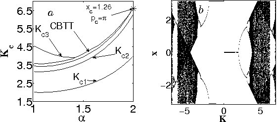
Figure 1: Bifurcations in the Standard $\alpha$-RL-family of maps: (a). Bifurcations in the fractional Standard Map for $1<\alpha<2$. Below $K=K_{c1}$ curve $(0,0)$ fixed point is stable. It becomes unstable at $K=K_{c1}$ and gives birth to the antisymmetric $T=2$ sink which is stable for $K_{c1}<K<K_{c2}$. A pair of $T=2$ sinks with $x_{n+1}=x_{n}-\pi$, $p_{n+1}=-p_{n}$ is stable in the band above $K=K_{c2}$ curve. Cascade of bifurcations type trajectories (CBTTs) appear and exist in the narrow band which ends at the cusp at the top right corner of the figure. $(x_{c},p_{c})$ is the point at which the Standard Map’s ($\alpha=2$) $T=2$ elliptic points with $x_{n+1}=x_{n}-\pi$, $p_{n+1}=-p_{n}$ become unstable and bifurcate. In the area below $K_{c3}$ (above the CBTT band) the chaotic attractor is restricted to a band which width is less than $2\pi$. On the upper curves and above them the full phase space is chaotic; (b). Bifurcation diagram for the one-dimensional Standard Map (59).

Low K ($K\leq K_{c1}$). Fixed point $(0,0)$, which is a sink for $1<\alpha<2$ when

$$K\leq K_{c1}(\alpha)=\frac{2\Gamma(\alpha)}{V_{\alpha l}},$$ (57)

where

$$V_{\alpha l}=\sum_{k=1}^{\infty}(-1)^{k+1}V_{\alpha}^{1}(k),$$ (58)

for $\alpha=2$ converges to the elliptic point which is stable for $K\leq K_{c1}(2)=4$.

The one-dimensional Standard Map ($\alpha=1$) can be written as

$$x_{n+1}=x_{n}-K\sin(x_{n}),\ \ \ \ ({\rm mod}\ 2\pi),$$ (59)

which is a particular form of the Circle Map with zero driving phase. It has attracting fixed points $2\pi n$ for $0<K\leq K_{c1}(1)=2$ and $\pi+2\pi n$ when $-2\leq K<0$ (see Fig. 1b).

Antisymmetric period 2 point ($K_{c1}\leq K\leq K_{c2}$). $1<\alpha<2$ antisymmetric period 2 sink

$$p_{n+1}=-p_{n},\ \ x_{n+1}=-x_{n}$$ (60)

exists for $K>K_{c1}(\alpha)$ and is stable for

$$K_{c1}(\alpha)\leq K\leq K_{c2}(\alpha),\ \ {\rm where}\ \ K_{c2}(\alpha)=\frac{\pi\Gamma(\alpha)}{V_{\alpha l}}.$$ (61)

For the regular Standard Map it gives a well known result $K_{c1}(2)=4\leq K\leq K_{c2}(2)=2\pi$. For $\alpha=1$ stability analysis produces $K_{c1}(1)=2\leq|K|\leq K_{c2}(2)=\pi$ for the stability of the period two sink $x_{n+1}=2\pi m-x_{n}$.

$x_{n+1}=x_{n}+\pi$ period 2 point ($K\geq K_{c2}$ below the CBTT band). For $1<\alpha<2$ two periodic sinks

$$p_{n+1}=-p_{n},\ \ x_{n+1}=x_{n}+\pi$$ (62)

appear at $K=K_{c2}$ and exist for $K\geq K_{c2}$ below the CBTT band. For the Standard Map the corresponding elliptic points are stable when $2\pi\leq K\leq 6.59$. For $\alpha=1$ $x_{n+1}=x_{n}+\pi$ sinks are stable when $\pi\leq|K|\leq\sqrt{\pi^{2}+2}\approx 3.445$.

Cascade of bifurcations band.

At $K\approx 6.59$ in the Standard Map an elliptic-hyperbolic point transition, when $T=2$ points become unstable and stable $T=4$ elliptic points, appear occurs. Further increase in $K$ results in the period doubling cascade of bifurcations which leads to the disappearance of the corresponding islands of stability in the chaotic sea at $K\approx 6.6344$. The cusp in Fig. 1a points to approximately this spot ($\alpha=2,K\approx 6.63$). Inside the band, leading to the cusp, a new type of attractors appears: cascade of bifurcations type trajectories (see Fig. 2).

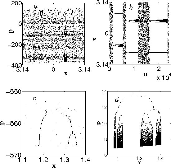
Figure 2: Cascade of bifurcations type trajectories: (a). $\alpha=1.65,K=4.5$; one intermittent trajectory in phase space; (b). Time dependence of the coordinate $x$ ($x$ of $n$) for the case (a); (c). $\alpha=1.98,K=6.46$; zoom of a small feature for a single intermittent trajectory in phase space; (d). $\alpha=1.1,K=3.5$; a single trajectory enters the cascade after a few iterations and stays there during 500000 iterations.

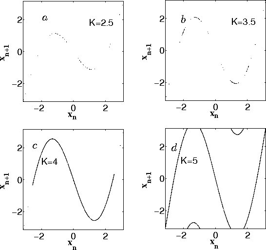
Figure 3: Attractors in one-dimensional Standard Map - $x_{n}$ vs. $x_{n+1}$ plots: (a). $K=2.5$; antisymmetric $T=2$ sink; (b). $K=3.5$; $T=4$ trajectory; (c). $K=4$; proper attractor (width of the chaotic area is less than $2\pi$); (d). $K=5$; improper attractor (width of the chaotic area is $2\pi$).

In the CBTTs period doubling cascade of bifurcations occurs on a single trajectory without any change in the map parameter. A typical CBTT’s behavior is similar to the Hamiltonian dynamics in the presence of sticky islands: occasionally a trajectory enters a CBTT and then leaves it entering the chaotic sea (Fig. 2a,b). As $\alpha$ decreases the relative time trajectories spend in CBTTs increases. Near the cusp (Fig. 2c) CBTTs are barely distinguishable and the relative time trajectories spend in CBTTs is small. When $\alpha$ is close to one, a trajectory enters a CBTT after a few iterations and stays there over the longest computational time we were running our codes - 500000 iterations. For $\alpha=1$ sequence of bifurcations: $T=4$ at $K\approx 3.445$, $T=8$ at $K\approx 3.513$, $T=16$ at $K\approx 3.526$, and so on leads to the transition to chaos at $K\approx 3.532$. Single antisymmetric $T=2$ ($K=2.5$), $T=4$ ($K=3.5$), and two chaotic trajectories ($K=4$ and $K=5$) are presented in Fig. 3.

$K<K_{c3}$ above the CBTT band - $x$-proper attractor

In the one-dimensional map with $K>0$ the full phase space becomes involved in chaotic motion (we’ll call this case “improper attractor”) when the maximum of the function $f_{K}(x)=x-K\sin x$ is equal to $\pi$ which occurs at $K_{max}=4.603339$ when $x_{max}=-1.351817$. This is the point at which $K=K_{c3}(\alpha)$ curve on Fig. 1a hits the $\alpha=1$ line. In the area between $K=K_{c3}(\alpha)$ curve and the upper border of the CBTT band the fractional attractors are proper (see Fig. 4)

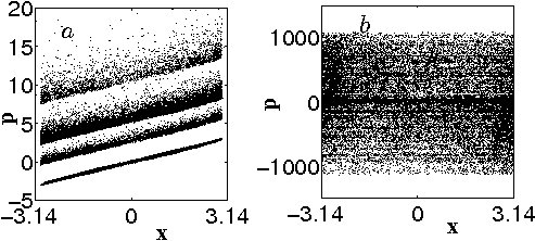
Figure 4: Proper and improper attractors. 3000 iterations on ten trajectories with the initial conditions $x_{0}=0$, $p_{0}=0.001+1.65i$, $i=0,1,...9$: (a). A proper attractor for $K=4.2$, $\alpha=1.1$; (b). An improper attractor for $K=4.4$, $\alpha=1.1$.

$K=2\pi n$ accelerator mode attractor

The regular Standard Map has a set of bands for $K$ above $2\pi n$ of the accelerator mode sticky islands in which momentum increases proportionally to the number of iterations $n$ and coordinate increases as $n^{2}$. The role of the accelerator mode islands (for $K$ above $2\pi$) in the anomalous diffusion and the corresponding fractional kinetics is well investigated (see, for example, Niyazov ; ZasBook2005 ).

In the one-dimensional map the corresponding bands demonstrate cascades of bifurcations (see Fig. 1b) for $|K|$ above $2\pi|n|$. The acceleration in those bands is zero and $x$ increases proportionally to $n$.

The case $1<\alpha<2$ is not fully investigated. The accelerator mode islands evolve into the accelerator mode (ballistic) attracting sticky trajectories when $\alpha$ is reduced from $2$ for the values of $K$ which increase with the decrease in $\alpha$ (Fig. 5b). When the value of $\alpha$ increases from 1, the corresponding ballistic attractors evolve into the cascade of bifurcation type ballistic trajectories (see Fig. 5a) for the values of $K$ which decrease with the increase in $\alpha$. This could mean that corresponding features in the one- and two-dimensional maps (at least for $K=2\pi$) are not connected by the continued change in $\alpha$.

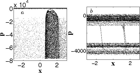
Figure 5: Accelerator mode attractors. 25000 iterations on a single trajectory with the initial conditions $x_{0}=0$, $p_{0}=0.1$: (a). CBTT-type accelerator mode attractor for $K=5.7$, $\alpha=1.03$; (b). Accelerator mode attractor for $K=7.6$, $\alpha=1.97$.

3.2.2 Standard $\alpha$-RL-family for $2\leq\alpha\leq 3$

$\alpha=3$ Universal and Standard Maps

Following Eqs. (39),(42), and (43), and assuming $T=1$ the three-dimensional universal map can be written as ($y=p$, $z=\dot{p}$)

$$x_{n+1}=\frac{z_{0}}{2}(n+1)^{2}+y_{0}(n+1)+x_{0}-\frac{1}{2}\sum^{n}_{k=0}G(x_{k})(n-k+1)^{2},$$ (63)

$$y_{n+1}=z_{0}(n+1)+y_{0}-\sum^{n}_{k=0}G(x_{k})(n-k+1),$$ (64)

$$z_{n+1}=z_{0}-\sum^{n}_{k=0}G(x_{k}),$$ (65)

which can be reduced to

$$x_{n+1}=x_{n}-\frac{1}{2}G(x_{n})+y_{n}+\frac{1}{2}z_{n},$$

$$y_{n+1}=-G(x_{n})+y_{n}+z_{n},$$

$$z_{n+1}=-G(x_{n})+z_{n},$$ (66)

or

$$x_{n+1}=x_{n}+y_{n+1}-\frac{1}{2}z_{n+1},$$

$$y_{n+1}=y_{n}+z_{n+1},$$

$$z_{n+1}=-G(x_{n})+z_{n},$$ (67)

which is a volume preserving map.

Let’s assume that this map has a fixed point $(x_{0},y_{0},z_{0})$. Then $z_{0}=y_{0}=G(x_{0})=0$ and stability of this point can be analyzed considering the eigenvalues of the matrix (corresponding to the tangent map)

$$\left(\begin{array}[]{ccc}1-0.5\dot{G}(x_{0})&1&0.5\\ -\dot{G}(x_{0})&1&1\\ -\dot{G}(x_{0})&0&1\end{array}\right).$$

The only case in which the fixed point is stable is $\dot{G}(x_{0})=0$, when $\lambda_{1}=\lambda_{2}=\lambda_{3}=1$.

For the three-dimensional Standard Map with $G(x)=K\sin(x)$

$$x_{n+1}=x_{n}+y_{n+1}-\frac{1}{2}z_{n+1},\ \ ({\rm mod}\ 2\pi),$$

$$y_{n+1}=y_{n}+z_{n+1},\ \ ({\rm mod}\ 2\pi),$$

$$z_{n+1}=-K\sin(x_{n})+z_{n},\ \ ({\rm mod}\ 4\pi)$$ (68)

it means that fixed points $(2\pi n,2\pi m,4\pi k)$ and $(2\pi n+\pi,2\pi m,4\pi k)$ , $n\in\mathbb{Z}$, $m\in\mathbb{Z}$, $k\in\mathbb{Z}$, are unstable for all $K\neq 0$. Ballistic points $K\sin(x)=-4\pi n$, $y=2\pi m$, $z=4\pi k$, which appear for $|K|\geq 4\pi$, are also unstable.

Stability of $T=2$ points is defined by the eigenvalues of the matrix

$$\left(\begin{array}[]{ccc}1-0.5K\cos x_{1}&1&0.5\\ -K\cos x_{1}&1&1\\ -K\cos x_{1}&0&1\end{array}\right)\times\left(\begin{array}[]{ccc}1-0.5K\cos x_{2}&1&0.5\\ -K\cos x_{2}&1&1\\ -K\cos x_{2}&0&1\end{array}\right).$$

For the stable (on the torus) period two point

$$z_{1},\ \ y_{1}=\frac{z_{1}}{2}-\pi(2n+1),\ \ K\sin x_{1}=2z_{1},$$

$$z_{2}=-z_{1},\ \ y_{2}=-\frac{z_{1}}{2}-\pi(2n+1),\ \ x_{2}=x_{1}-\pi(2n-1),$$ (69)

where $n\in\mathbb{Z}$, the eigenvalues are

$$\Bigl{\{}1,\ \ \frac{1}{8}(8-K^{2}\cos^{2}x_{1}\pm K\cos x_{1}\sqrt{K^{2}\cos^{2}x_{1}-16})\Bigr{\}}$$ (70)

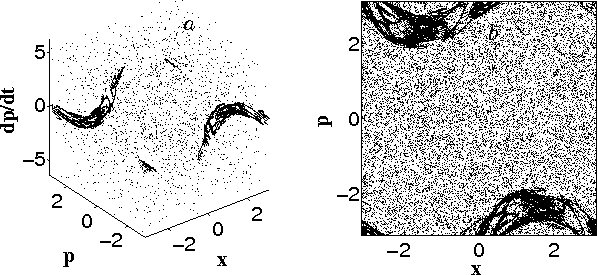
Figure 6: Phase space of the 3D Standard Map (68) for $K=3$: (a). Phase space in three dimensions; (b). Projection of the phase space on the $x$-$y$ plane.

Stable $T=2$ points exist along a line defined by Eqs. (69) for all values of $z$ satisfying the condition

$$K^{2}-16<4z^{2}<K^{2}.$$ (71)

An example of phase space for $K=3$ in three dimensions and its projection on the $x$-$y$ plane is given in Fig. 6. In this case $T=2$ points are stable for $-1.5<z<1.5$ and the space around the line of stability presents a series of islands (invariant curves), islands around islands, and separatrix layers. As $K$ goes to zero, the volume of the regular motion shrinks. For small values of $K$ the line of the stable $T=2$ points exists for $-K/2<z<K/2$. A different form of the 3D volume preserving Standard Map was introduced and investigated in details in DM .

$2<\alpha\leq 3$

Assuming $G(x)=K\sin(x)$ and $T=1$ in Eqs. (50)-(52), the FSMRL for $2<\alpha\leq 3$ can be written as

$$p^{1}_{n+1}=p^{1}_{n}-K\sin(x_{n}),$$ (72)

$$p_{n+1}=p^{1}_{n}+p_{n}-K\sin(x_{n}),\ \ ({\rm mod}\ 2\pi),$$ (73)

$$x_{n+1}=\frac{p_{0}}{\Gamma(\alpha-1)}(n+1)^{\alpha-2}+\frac{1}{\Gamma(\alpha)}\sum^{n}_{k=0}p^{1}_{k+1}V^{1}_{\alpha}(n-k+1),$$ (74)

$$\ \ ({\rm mod}\ 2\pi).$$

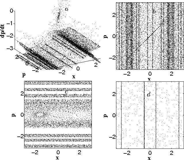
Figure 7: FSM for $2<\alpha<3$: (a). 3D phase space for $K=1$, $\alpha=2.01$ obtained on a single trajectory with $x_{0}=p_{0}=0$ and $p^{1}_{0}=0.01$; (b). Projection of the phase space in (a) on the $x$-$y$ plane; (c). Projection of the phase space for $K=0.2$, $\alpha=2.01$, $x_{0}=p_{0}=0$ on the $x$-$y$ plane obtained using 20 trajectories with different initial values of $p^{1}_{0}$; (d). The same as in (c), but for $K=4$ and $\alpha=2.9$.

In our simulations we did not find a stable fixed point even for small values of $K$ (see Figs. 7 (c). Simulations show that for this map there are attractors in the form of the attracting multi-period lines with constant $x$ (see Fig. 7 (a), (b), and (d)). For most of the values of the map parameters the phase space is highly chaotic.

This case and the transition from the 2D Standard Map to the 3D Standard Map, as well as 3D Standard Map, is not yet fully investigated.

3.2.3 Logistic $\alpha$-RL-family for $1\leq\alpha\leq 3$

Case $\alpha=1$ is probably the best investigated map - the regular Logistic Map. For $1<\alpha\leq 2$ it can be written as

$$p_{n+1}=p_{n}+Kx_{n}(1-x_{n})-x_{n},$$ (75)

$$x_{n+1}=\frac{1}{\Gamma(\alpha)}\sum^{n}_{k=0}p_{k+1}V^{1}_{\alpha}(n-k+1),$$ (76)

which for $\alpha=2$ can be reduced to

$$p_{n+1}=p_{n}+Kx_{n}(1-x_{n})-x_{n},$$ (77)

$$x_{n+1}=x_{n}+p_{n+1}.$$ (78)

This map is similar to the original area preserving quadratic map considered by Hénon Henon69 (for a recent review see book ZeraS2010 ). As for the Standard $\alpha$-RL-family, for the Logistic $\alpha$-RL-family of maps we are interested in the stable fixed and periodic points in order to follow their evolution as a function of $\alpha$. For $-3<K<1$ $(0,0)$ fixed point of the 2D Logistic Map is stable. At $K=1$ it becomes unstable but fixed point $((K-1)/K,0)$ becomes stable. This point is stable for $1<K<5$. At $K=5$ a bifurcation occurs and this stable fixed point changes to a couple of $T=2$ stable points

$$x=\frac{K+3\pm\sqrt{(K+3)(K-5)}}{2K},\ \ p=\pm\frac{\sqrt{(K+3)(K-5)}}{2K}.$$ (79)

For $2<\alpha\leq 3$ the map can written as

$$p^{1}_{n+1}=p^{1}_{n}+Kx_{n}(1-x_{n})-x_{n},$$ (80)

$$p_{n+1}=p^{1}_{n}+p_{n}+Kx_{n}(1-x_{n})-x_{n},$$ (81)

$$x_{n+1}=\frac{p_{0}}{\Gamma(\alpha-1)}(n+1)^{\alpha-2}+\frac{1}{\Gamma(\alpha)}\sum^{n}_{k=0}p^{1}_{k+1}V^{1}_{\alpha}(n-k+1),$$ (82)

which for $\alpha=3$ can be reduced to

$$x_{n+1}=x_{n}+y_{n+1}-\frac{1}{2}z_{n+1},$$

$$y_{n+1}=y_{n}+z_{n+1},$$

$$z_{n+1}=Kx_{n}(1-x_{n})-x_{n}+z_{n}.$$ (83)

3D quadratic volume preserving maps were investigated in Moser1994 ; LoMeiss1998 . Everything stated in Subsection 3.2.2 for the 3D Universal Map is still valid for the 3D Logistic Map. More on the Logistic $\alpha$-RL-family of maps will be presented in the part II of the article.

3.3 Caputo Universal Map

The Logistic and Standard $\alpha$-RL-families give identical zeros in the case $\alpha<1$. This is not the case for the Logistic and Standard $\alpha$-Caputo-families (FLMC and FSMC), for which the condition $x_{0}=0$ can be removed. In order to get some insight into the origin of one of the most interesting features of fractional maps - CBTTs, we complete this part of the paper with the analysis of the simplest case of CBTTs in the Logistic and Standard $\alpha$-Caputo-families of the maps when $\alpha<1$. But let’s first introduce the Caputo Universal Map.

Similar to (34) in the case of the Caputo fractional derivative we have

$${}_{0}^{C}D^{\alpha}_{t}x(t)+G(x(t-\Delta T))\sum^{\infty}_{n=-\infty}\delta\Bigl{(}\frac{t}{T}-(n+\varepsilon)\Bigr{)}=0,\ \ \varepsilon>\Delta>0,$$ (84)

where $\varepsilon\rightarrow 0$, $0\leq N-1<\alpha\leq N$, and the initial conditions

$$(D^{k}_{t}x)(0+)=b_{k},\ \ k=0,...,N-1.$$ (85)

The left-sided Caputo fractional derivative ${}_{0}^{C}D^{\alpha}_{t}x(t)$ defined for $t>0$ Podlubny ; SKM ; KST as

$${}_{0}^{C}D^{\alpha}_{t}x(t)=_{0}I^{n-\alpha}_{t}\ D^{n}_{t}x(t)=$$

$$\frac{1}{\Gamma(n-\alpha)}\int^{t}_{0}\frac{D^{n}_{\tau}x(\tau)d\tau}{(t-\tau)^{\alpha-n+1}}\quad(n-1<\alpha\leq n).$$ (86)

This problem is equivalent to the following Volterra integral equation ($t>0$) TarasovBook2011 ; KST

$$x(t)=\sum^{N-1}_{k=0}\frac{b_{k}}{k!}t^{k}$$

$$-\frac{1}{\Gamma(\alpha)}\int^{t}_{0}d\tau\frac{G(x(\tau-\Delta T))}{(t-\tau)^{1-\alpha}}\sum^{\infty}_{k=-\infty}\delta\Bigl{(}\frac{\tau}{T}-(k+\varepsilon)\Bigr{)}.$$ (87)

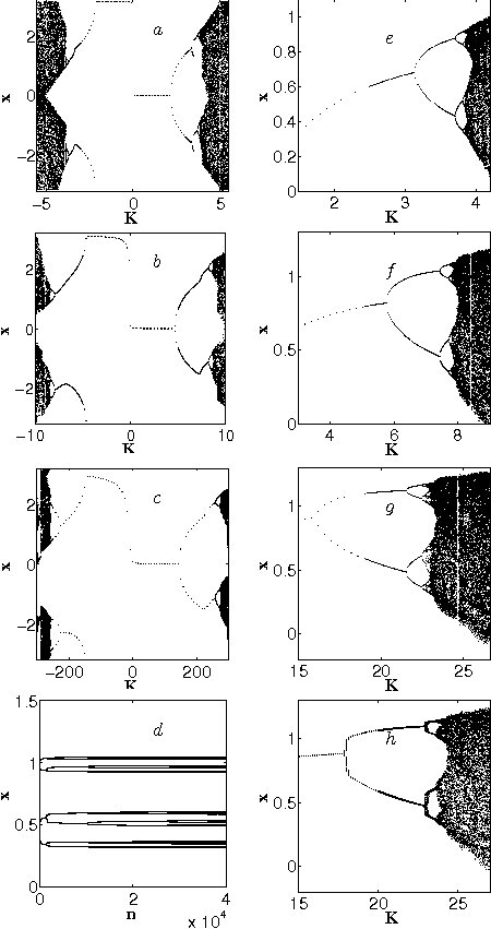
Figure 8: Cascades of bifurcations and CBTTs in Standard and Logistic $\alpha$-Caputo-families (FSMC and FLMC) for $0<\alpha<1$: (a). Cascade of bifurcations for the FSMC (91) with $\alpha=0.8$ obtained after performing 10000 iterations on a single trajectory with $x_{0}=0.1$ for various values of $K$; (b). The same as in (a) but for $\alpha=0.3$; (c). The same as in (a) but for $\alpha=0.01$; (d). A single CBTT for the FLMC with $\alpha=0.4$, $K=6.075$, and the initial condition $x_{0}=0.1$; (e). The same as in (a) but for the FLMC (92); (f). The same as in (b) but for the FLMC; (g). The same as in (e) but for $\alpha=0.1$; (h). The same as in (g) but after 100 iterations.

Then we also have for $t>0$

$$x(t)=\sum^{N-1}_{k=0}\frac{b_{k}}{k!}t^{k}$$

$$-\frac{T}{\Gamma(\alpha)}\sum^{[t/T-\varepsilon]}_{k=0}\frac{G(x((k+\varepsilon)T))}{(t-(k+\varepsilon)T)^{1-\alpha}}\Theta(t-(k+\varepsilon)T)$$ (88)

and the map

$$x_{n+1}=\sum^{N-1}_{k=0}\frac{b_{k}}{k!}[T(n+1)]^{k}$$

$$-\frac{T^{\alpha}}{\Gamma(\alpha)}\sum^{n}_{k=0}G(x_{k})(n-k+1)^{\alpha-1},$$ (89)

which for $0<\alpha<1$, assuming $T=1$, gives

$$x_{n+1}=x_{0}-\frac{1}{\Gamma(\alpha)}\sum^{n}_{k=0}G(x_{k})(n-k+1)^{\alpha-1}.$$ (90)

3.3.1 Standard and Logistic $\alpha$-Caputo-families for $0<\alpha<1$

For $0<\alpha<1$ the Standard $\alpha$-Caputo-family can be written as

$$x_{n}=x_{0}-\frac{K}{\Gamma(\alpha)}\sum^{n-1}_{k=0}\frac{\sin{x_{k}}}{(n-k)^{1-\alpha}},\ \ ({\rm mod}\ 2\pi)$$ (91)

and the Logistic $\alpha$-Caputo-family as

$$x_{n}=x_{0}+\frac{1}{\Gamma(\alpha)}\sum^{n-1}_{k=0}\frac{Kx_{k}(1-x_{k})-x_{k}}{(n-k)^{1-\alpha}}.$$ (92)

As one may see, from (91), (92), and Figs. 8 (a)-(c) and (e)-(g) a decrease in $\alpha$ and corresponding decrease in the weights of the earlier states (decrease in the memory effects) leads to the shift of the bifurcation curves to the higher values of the maps’ parameter $K$, which means increased stability. When $\alpha\rightarrow 1$ the bifurcation curves converge to the curve in Fig. 1b for the FSM and to the well known bifurcation curve for the Logistic Map in the case of the FLM.

For the values of $K$ at which periodic $T>2$ stable points exist the individual trajectories are the CBTTs (see Fig. 8d), where an increase in the number of the map iterations leads to the change in the map’s stability properties. These are the simplest so far examples of the maps with the CBTTs. As a result, the FSMC and the FLMC can be used as the simplest models for studying the CBTT phenomenon.

The presence of CBTTs leads to the dependence of the the bifurcation curve on the number of iterations. From Figs. 8 (g) and (h) one may see that with the increase in the number of iterations in the the FLMC the bifurcation curve becomes more pronounced and shifts to the left (to the lower values of the map parameter $K$).

4 Conclusion

Differential equations with the integer order derivatives and the terms containing periodic delta-function shaped kicks are frequently used in science to model the behavior of real systems. They can be easily integrated over an integer number of periods in order to obtain maps, which then can be numerically investigated in order to derive the general properties of the original systems. Well known examples of such maps are the Standard Map in physics and the Logistic Map in population biology. In this paper we proposed continuation of the integer maps into the area of the fractional maps corresponding to the arbitrary positive values of the orders of the fractional derivatives in the original differential equations. We introduced the notions of the Riemann-Lioville and Caputo $\alpha$-families of maps, which depend on a single parameter - order of the fractional derivative $\alpha>0$. Increase in $\alpha$ corresponds to the increase in the dimension of the space (which can be important in physical systems) and to the increase in the memory effects (the weights of the earlier states increase with the increase in $\alpha$), which is important in population biology (information about past states of the system can be recorded in the DNA of individuals, the society as a whole can regulate evolution of the population by introducing laws based on the past experience).

Our first results show that increase in $\alpha$ leads to more a more complex behavior of the system. As $\alpha\rightarrow 0$ any memory of the past disappear and the system stabilizes at zero for the Riemann-Lioville families or at constant value for the Caputo families. For $0<\alpha<1$ the behavior of the systems is qualitatively similar to the behavior of the system with $\alpha=1$ with stability reducing as $\alpha\rightarrow 1$. Within the bifurcation ($T>2$) band of the parameter values fractional systems evolve as CBTTs.

For $1<\alpha<2$ the systems become two-dimensional and their phase space contains different kinds of arttractors like sinks, chaotic attractors, CBTTs, and intermittent CBTTs.

Case $2<\alpha<3$ requires more thorough investigation. Our preliminary results show the existence of very complicated three-dimensional attractors and instability of the fixed points. In general, as $\alpha$ increases, the systems become more and more chaotic.

In the second part of this paper we’ll present more results on the fractional Logistic Map with $\alpha>1$, the fractional Standard Map with $\alpha>2$, and the CBTTs.

References

- (1) V. E. Tarasov, G. M. Zaslavsky, Fractional equations of kicked systems and discrete maps, J. Phys. A 41 (2008) 435101.
- (2) V. E. Tarasov, Discrete map with memory from fractional differential equation of arbitrary positive order, J. Math. Phys. 50 (2009) 122703.
- (3) V. E. Tarasov, Differential equations with fractional derivative and universal map with memory, J. Phys. A 42 (2009) 465102.
- (4) V. E. Tarasov, Fractional Dynamics: Application of Fractional Calculus to Dynamics of Particles, Fields and Media, Springer, HEP, 2011.
- (5) M. Edelman, V. E. Tarasov, Fractional standard map, Phys. Let. A 374 (2009) 279–285.
- (6) V. E. Tarasov, M. Edelman, Fractional dissipative standard map, Chaos 20 (2010) 023127.
- (7) M. Edelman, Fractional Standard Map: Riemann-Liouville vs. Caputo, Commun. Nonlin. Sci. Numer. Simul. 16 (2011) 4573–4580.
- (8) M. Edelman, L. A. Taieb, New types of solutions of non-linear fractional differential equations, in: Advances in Harmonic Analysis and Operator Theory; Series: Operator Theory: Advances and Applications; Eds: A. Almeida, L. Castro, F.-O. Speck; 17 pp, (Birkh user, 2012) (accepted).
- (9) D. K. Arrowsmith, C. M. Place, An introduction to dynamical systems, Cambridge University Press, Cambridge, 1990.
- (10) M. Feigenbaum, Quantitative universality for a class of nonlinear transformations, J. Stat. Phys. 19 (1978) 25–52.
- (11) O. E. Lanford, A computer assisted proof of the Feigenbaum conjectures, Bull. am. Math. Soc. 6 (1982) 427–434.
- (12) E. B. Vul, Y. G. Sinai, K. M. Khanin, Feigenbaum universality and thermodynamic formalism, Russ. Math. Surv. 39 (1984) 1–40.
- (13) P. Cvitanovic, Universality in chaos, Adam Hilger, Bristol, 1989.
- (14) K. M. Briggs, Feigenbaum Scaling in Discrete Dynamical Systems, Ph.D. thesis. Melbourne, Australia: University of Melbourne, 1997; http://keithbriggs.info/thesis.html.
- (15) A. Fulinski, A. S. Kleczkowski, Nonlinear maps with memory, Physica Scripta 35 (1987) 119–122.
- (16) E. Fick, M. Fick, G. Hausmann, Logistic equation with memory, Phys. Rev. A 44 (1991) 2469–2473.
- (17) K. Hartwich, E. Fick, Hopf bifurcations in the logistic map with oscillating memory, Phys. Lett. A 177 (1993) 305–310.
- (18) M. Giona, Dynamics and relaxation properties of complex systems with memory, Nonlinearity 4 (1991) 911–925.
- (19) J. A. C. Gallas, Simulating memory effects with discrete dynamical systems, Physica A 195 (1993) 417–430; Erratum. Physica A 198 (1993) 339–339.
- (20) A. A. Stanislavsky, Long-term memory contribution as applied to the motion of discrete dynamical system, Chaos 16 (2006) 043105.
- (21) I. Podlubny, Fractional Differential Equations, Academic Press, San Diego, 1999.
- (22) R. M. May, Simple mathematical models with very complicated dynamics, Nature 261 (1976) 459–467.
- (23) R. Alonso-Sanz, Extending the parameter interval in the logistic map with memory, Int. J. Bifurc. Chaos 21 (2011) 101–111.
- (24) F. Bauer, C. Castillo-Chavez, Mathematical Models in Population Biology and Epidemiology, Springer, New York, 2001.
- (25) Y. Takeuchi, Y. Iwasa, K. Sato (Eds), Mathematics for Life Science and Medicine, Springer, Berlin, Heidelberg, New York, 2007.
- (26) A. Ausloos, M. Dirickx (Eds), The Logistic Map and the Route to Chaos, Springer, Berlin, Heidelberg, New York, 2006.
- (27) S. G. Samko, A. A. Kilbas, O. I. Marichev, Fractional Integrals and Derivatives Theory and Applications, Gordon and Breach, New York, 1993.
- (28) A. A. Kilbas, H.M. Srivastava, J. J. Trujillo, Theory and Application of Fractional Differential Equations, Elsevier, Amsterdam, 2006.
- (29) A. A. Kilbas, B. Bonilla, J. J. Trujillo, Nonlinear differential equations of fractional order is space of integrable functions, Doklady Mathematics 62 (2000) 222–226, Translated from Doklady Akademii Nauk 374 (2000) 445–449 (in Russian).
- (30) A. A. Kilbas, B. Bonilla, J. J. Trujillo, Existence and uniqueness theorems for nonlinear fractional differential equations, Demonstratio Mathematica 33 (2000) 583–602.
- (31) B. V. Chirikov, A universal instability of many dimensional oscillator systems, Phys. Rep. 52 (1979) 263–379.
- (32) A. J. Lichtenberg, M. A. Lieberman, Regular and Chaotic Dynamics, Springer, Berlin, 1992.
- (33) G. M. Zaslavsky, M. Edelman, B. A. Niyazov, Self-similarity, renormalization, and phase space nonuniformity of Hamiltonian chaotic dynamics, Phys. Rev. E 56 (1997) 5310–5320.
- (34) G. M. Zaslavsky, Hamiltonian Chaos and Fractional Dynamics, Oxford, Oxford University Press, 2005.
- (35) H. R. Dullin and J. D. Meiss, Resonances and Twist in Volume-Preserving Maps, SIAM J. Appl. Dyn. Sys. 11 (2012) 319–359.
- (36) M. Hénon, Numerical study of quadratic area-preserving mappings, Q. Appl. Math. XXVII, no.3 (1969) 291–312.
- (37) E. Zeraoulia, J. C. Sprott, 2-D Quadratic Maps and 3-D ODE Systems: A Rigorous Approach, World Scientific, Singapore, 2010.
- (38) J. Moser, On quadratic symplectic mappings, Math. Z. 216 (1994) 417–430.
- (39) H. E. Lomeli and J. D. Meiss, Quadratic volume-preserving maps, Nonlinearity, 11 (1998) 557–574.