Role of the spectral shape of quantum correlations in two-photon virtual-state spectroscopy

Abstract

It is controversial what is the true role of entanglement in two-photon virtual-state spectroscopy [Saleh et al, Phys. Rev. Lett. 80, 3483, 1998], a two-photon absorption spectroscopic technique that can retrieve information about the energy level structure of an atom or a molecule. The consideration of closely related techniques, such as multidimensional pump-probe spectroscopy [Roslyak et al, Phys. Rev. A 79, 063409, 2009] suggests that spectroscopic information might also be retrieved by using uncorrelated pairs of photons. Here we show that this is not the case. In the two-photon absorption process, the ability to obtain information about the energy level structure of a medium depends on the spectral shape of existing temporal (frequency) correlations between the absorbed photons. In fact, it is a combination of both, the presence of frequency correlations (entanglement) and its specific spectral shape, which makes the realization of two-photon virtual-state spectroscopy possible. This result helps for selecting the type of two-photon source that needs to be used in order to experimentally perform the two-photon virtual-state spectroscopy technique.

1 Introduction

The process of two-photon absorption (TPA), the light-induced transition between two energy levels of a medium mediated by the absorption of two photons, is a building block of some technologies aimed at probing the structure of atoms and molecules, such as two-photon microscopy [1] and two-photon spectroscopy [2]. In particular, nonlinear two-photon spectroscopy has become an invaluable tool [3], where the capability of TPA is exploited to obtain information about a sample that would not be accessible otherwise.

With the advent of light sources that generate entangled photon pairs [4], new phenomena in TPA processes have been unveiled. The linear dependence of the two-photon absorption rate on the photon flux [5], two-photon induced transparency [6], virtual-state spectroscopy [7, 8] and the selectivity of double-exciton states of chromophore aggregates [9] are effects that have been attributed to the presence of entanglement. However, the link between entanglement and the new effect observed is sometimes blur. So, might not be the ultimate cause of some of these effects an accompanying characteristic unrelated to its entangled nature? This is the case of certain effects that, when first described, were attributed to the existence of frequency entanglement between pairs of photons. For instance, Nasr et al. [10] demonstrated a new scheme, based on entanglement, to erase effects due to second-order chromatic dispersion in optical coherence tomography, thus increasing the resolution of the system. Later, the work in [11] showed that by appropriately introducing a phase conjugator element in the optical coherence tomography scheme, which produces a Gaussian-state light source with frequency anti-correlation, a similar effect could be achieved. In dispersion cancelation, an effect that is observed in the temporal domain, namely the broadening of the second-order correlation function of paired photons propagating in two different optical fibers, it was shown that it can be suppressed, provided that the group velocity dispersion parameters of both fibers are identical but opposite in sign, and that the photons are entangled [12, 13, 14]. However, it has been recently demonstrated that such effects could also be produced by frequency-correlated photons, which nonetheless might be non-entangled [15, 16].

Remote temporal modulation [17, 18], a similar effect to the dispersion cancelation described above, but observed in the frequency domain, describes the appearance of new frequency correlations when entangled paired photons are synchronously driven by two temporal modulators. In a similar manner to dispersion cancelation, if the two identical modulators are driven in opposite phases, their global effect is to negate each other, and the spectral correlations appear as those when no phase modulators are present. Again, it has been shown [16] that entanglement is not a requisite, and that the same effect can be observed using non-entangled optical beams bearing certain frequency correlations. All these examples illustrate the fact that the presence of entanglement is not the key enabling factor that allows the observation of dispersion cancelation and remote temporal modulation, but the existence of certain frequency correlations, a characteristic that takes place along the presence of entanglement, but it can also manifest without it.

In this paper, we consider one important spectroscopic application whose capabilities have been associated to the use of entangled photon pairs, namely two-photon virtual-state spectroscopy. The importance of this technique resides in the fact that, unlike commonly used two-photon absorption spectroscopy techniques, where pulsed and tunable sources are required, it is implemented by carrying out continuous-wave absorption measurements without changing the wavelength of the source [7, 8]. Unfortunately, this technique has not been broadly applied because the ease with which it can be performed is limited by the low efficiency of spontaneous down conversion in nonlinear crystals. However, with the advent of ultrahigh flux sources of entangled photons [19], this technique may open new research directions towards ultrasensitive detection in chemical and biological systems [20, 21].

The absorption of two photons by an atom or a molecule induces a transition between two of its energy levels that match the overall energy of the incident photons. The quantum mechanical calculation of the TPA transition probability shows that its value can be understood as a weighted sum of many energy non-conserving atomic transitions (virtual-state transitions) [22, 23] between energy levels. Then, the virtual-state transitions, a signature of the medium, can be revealed experimentally by introducing a delay between the two absorbed photons, and averaging over different experimental realizations with different temporal correlations between the photons [7]. Can we retrieve the sought-after information (energy level structure) with any type of frequency correlations between the photons? It has been suggested that spectroscopic information resident in the TPA signal in multidimensional pump-probe spectroscopy [24] is essentially the same, regardless of the existence or not of correlations between the photons absorbed. As stated recently in [9], it remains however an open question, to what extent these effects constitute genuine entanglement effects and whether they can be reproduced, for instance, by shaped or stochastic classical pulses.

To unveil the true role of entanglement in virtual-state spectroscopy, we make use of two ingredients. First, we apply a full quantum formalism to the two-photon state, so we can identify clearly the amount of entanglement existing between the photons. Secondly, we consider a general form of the two-photon state, which allows us to consider different types of correlations and spectral shapes of the photons.

We will show that the presence of entanglement does not guarantee the successful retrieval of spectroscopic information of the medium. In fact, it is the combination of entanglement and a specific shape of the frequency correlations between photons what makes the realization of two-photon virtual-state spectroscopy possible. This result is of great interest because it specifies the type of two-photon source that needs to be used in order to experimentally perform the two-photon virtual-state spectroscopy technique.

2 Light-matter interaction

Let us consider the interaction of a medium with a two-photon optical field $\left|\Psi\right>$, described by the interaction Hamiltonian $\hat{H}_{I}\left(t\right)=\hat{d}\left(t\right)\hat{E}^{\left(+\right)}\left(t\right)$, where $\hat{d}\left(t\right)$ is the dipole-moment operator and $\hat{E}^{\left(+\right)}\left(t\right)$ is the positive-frequency part of the electric-field operator, which reads as $\hat{E}^{\left(+\right)}\left(t\right)=\hat{E}^{\left(+\right)}_{1}\left(t\right)+\hat{E}^{\left(+\right)}_{2}\left(t\right)$. The electric field operators $\hat{E}^{\left(+\right)}_{1}\left(t\right)$ and $\hat{E}^{\left(+\right)}_{2}\left(t\right)$ can be written as

$$\hat{E}^{\left(+\right)}_{j}\left(t\right)=\int d\omega_{j}\sqrt{\frac{\hbar\omega_{j}}{4\pi\epsilon_{0}cA}}\hat{a}\left(\omega_{j}\right)\exp\left(-i\omega_{j}t\right),$$ (1)

where $c$ is the speed of light, $\epsilon_{0}$ is the vacuum permittivity, $A$ is the effective area of the field, and $\hat{a}\left(\omega_{j}\right)$ is the annihilation operator of a photonic frequency-mode with frequency $\omega_{j}$ bearing a specific spatial shape and polarization which, for the sake of simplicity, are not explicitly written.

The medium is initially in its ground state $\left|g\right>$ (with energy $\varepsilon_{g}$). The probability that the medium is excited to the final state $\left|f\right>$ (with energy $\varepsilon_{f}$), through a two-photon absorption process, is given by second-order time-dependent perturbation theory as [25]

$$P_{g\rightarrow f}=\left|\frac{1}{\hbar^{2}}\int_{-\infty}^{\infty}dt_{2}\int_{-\infty}^{t_{2}}dt_{1}\mbox{M}_{\hat{d}}\left(t_{1},t_{2}\right)\mbox{M}_{\hat{E}}\left(t_{1},t_{2}\right)\right|^{2},$$ (2)

with

$$\mbox{M}_{\hat{d}}\left(t_{1},t_{2}\right) = \left<f\right|\hat{d}\left(t_{2}\right)\hat{d}\left(t_{1}\right)\left|g\right>,$$ (3)

$$\mbox{M}_{\hat{E}}\left(t_{1},t_{2}\right) = \left<\Psi_{f}\right|\hat{E}^{\left(+\right)}\left(t_{2}\right)\hat{E}^{\left(+\right)}\left(t_{1}\right)\left|\Psi\right>,$$ (4)

where $\left|\Psi_{f}\right>$ denotes the final state of the optical field.

Equation (3) can be expanded in terms of virtual-state transitions, to obtain

$$\mbox{M}_{\hat{d}}\left(t_{1},t_{2}\right)= \sum_{j=1} D^{\left(j\right)}\exp\left[{-i\left(\varepsilon_{j}-i\kappa_{j}/2-\varepsilon_{f}\right)t_{2}}\right]$$ (5)

$$\times \exp\left[-i\left(\varepsilon_{g}-\varepsilon_{j}+i\kappa_{j}/2\right)t_{1}\right],$$

where $D^{\left(j\right)}=\left<f\right|\hat{d}\left|j\right>\left<j\right|\hat{d}\left|g\right>$ are the transition matrix elements of the dipole-moment operator. Equation (5) shows that the excitation of the medium occurs through intermediate states $\left|j\right>$, with complex energy eigenvalues $\varepsilon_{j}-i\kappa_{j}/2$, where $\kappa_{j}$ takes into account the natural linewidth of the intermediate states [26]. Also, we can write Eq. (4) as

$$\mbox{M}_{\hat{E}}\left(t_{1},t_{2}\right)=\left<\psi_{f}\right|\hat{E}_{2}^{\left(+\right)}\left(t_{2}\right)\hat{E}_{1}^{\left(+\right)}\left(t_{1}\right)\left|\psi_{i}\right>+\left<\psi_{f}\right|\hat{E}_{1}^{\left(+\right)}\left(t_{2}\right)\hat{E}_{2}^{\left(+\right)}\left(t_{1}\right)\left|\psi_{i}\right>,$$ (6)

where we have kept the terms in which only one photon from each field contributes to the overall two-photon excitation. The first term of Eq. (6) corresponds to the case in which the photon field $\hat{E}_{1}^{\left(+\right)}\left(t\right)$ interacts first, and $\hat{E}_{2}^{\left(+\right)}\left(t\right)$ interacts later. The remaining term describes the complementary case.

Since we are interested in a two-photon absorption process, we consider the initial state of the optical field as an arbitrary two-photon state, which can be written as [27]

$$\left|\Psi\right>=\int d\nu_{s}d\nu_{i}\Phi\left(\nu_{s},\nu_{i}\right)\hat{a}_{s}^{\dagger}\left(\nu_{s}+\omega_{s}^{0}\right)\hat{a}_{i}^{\dagger}\left(\nu_{i}+\omega_{i}^{0}\right)\left|0\right>,$$ (7)

where $s$ and $i$ stand for signal and idler photonic modes, $\nu_{j}=\omega_{j}-\omega_{j}^{0}$ ($j=s,i$) are the frequency deviations from the central frequencies $\omega_{j}^{0}$, and $\Phi\left(\nu_{s},\nu_{i}\right)$ is the joint spectral amplitude, or mode function, which fully describes the correlations and bandwidth of the two-photon state.

Finally, to quantify the degree of entanglement between the absorbed photons, we make use of the entropy of entanglement, defined as [28]

$$E=-\sum_{i}\lambda_{i}\mbox{log}_{2}\lambda_{i},$$ (8)

where $\lambda_{i}$ are the eigenvalues of the Schmidt decomposition of the joint spectral amplitude, i.e., $\Phi\left(\nu_{s},\nu_{i}\right)=\sum_{i}\sqrt{\lambda_{i}}f_{i}(\nu_{s})g(\nu_{i})$, with $f$ and $g$ corresponding to the Schmidt modes. It is worth remarking that the lack of entanglement between the pair of photons is characterized by a value of the entropy equal to zero.

3 Two-photon absorption transition probability

With the aim of recognizing in which situations virtual-state spectroscopy can be performed, we will compute the TPA transition probability of atomic hydrogen using different types of initial two-photon states. We have selected atomic hydrogen as model system, because it has been used in previous studies of virtual-state spectroscopy [25, 7] and it has been the subject of several one- and two-photon absorption experiments [29, 30, 31, 32]. In our calculations, we will focus on the $1s\rightarrow 2s$ two-photon transition. Due to quantum number selection rules [31], this transition takes place via intermediate $p$ states: $1s\rightarrow\left\{2p,3p,...,np\right\}\rightarrow 2s$, which are coupled to the $s$ states by real-valued transition matrix elements. The hydrogen atom energy levels are $\varepsilon_{n}=-13.6/n^{2}$ eV ($n=1,2,3,...$) and the natural linewidths of intermediate states $\kappa_{j}$ are taken from Refs. [29, 31]. We assume the condition $\varepsilon_{f}-\varepsilon_{g}=\omega_{s}^{0}+\omega_{i}^{0}$, and that the final state $2s$ is Lorentzian broadened with a radiative lifetime $1/\kappa_{f}=122$ ms [30], which is introduced in the model by averaging the TPA transition probability over a Lorentzian function of width $\kappa_{f}$ [26].

3.1 TPA transition probability with uncorrelated classical pulses

Let us consider first the case that has been studied in Ref. [24]. It corresponds to the situation in which the two absorbed photons are embedded into rectangular-shaped pulses of the same duration $T_{p}$, with a tunable time delay $\tau$ between them. This initial optical field can be represented by an uncorrelated two-photon state described by the normalized mode function

$$\Phi\left(\nu_{s},\nu_{i}\right)=\frac{T_{p}}{2\pi}\mbox{sinc}\left(T_{p}\nu_{s}/2\right)\mbox{sinc}\left(T_{p}\nu_{i}/2\right)\exp\left[i\left(\nu_{s}-\nu_{i}\right)\tau/2\right].$$ (9)

With the state given by Eq. (9), and making use of Eqs. (2), (5) and (6), we can write the TPA transition probability as

$$P_{g\rightarrow f}\left(T_{p};\tau\right)=\frac{\omega_{0}^{2}}{\hbar^{2}\epsilon_{0}^{2}c^{2}A^{2}T_{p}^{2}}\left|\sum_{j}D^{\left(j\right)}\left[I_{1}+I_{2}\right]\right|^{2},$$ (10)

where

$$I_{1}= \frac{\sin\left[\Delta\omega\left(T_{p}-\tau\right)/2\right]}{\Delta_{g}\Delta\omega}-\frac{\sin\left[\Delta_{f}\left(T_{p}-\tau\right)/2\right]\exp\left[{i\Delta_{g}\left(T_{p}+\tau\right)/2}\right]}{\Delta_{g}\Delta_{f}}$$ (11)

$$-\frac{2i\sin\left(\Delta_{g}T_{p}/2\right)\sin\left(\Delta_{f}\tau/2\right)\exp\left[-i\left(\Delta_{f}T_{p}-\Delta_{g}\tau\right)/2\right]}{\Delta_{g}\Delta_{f}},$$

$$I_{2}=\frac{\sin\left[\Delta\omega\left(T_{p}-\tau\right)/2\right]}{\Delta_{g}\Delta\omega}-\frac{\sin\left[\Delta_{f}\left(T_{p}-\tau\right)/2\right]\exp\left[{i\Delta_{g}\left(T_{p}-\tau\right)/2}\right]}{\Delta_{g}\Delta_{f}},$$ (12)

with $\Delta_{f}=\varepsilon_{j}-i\kappa_{j}/2-\varepsilon_{f}+\omega_{0}$, $\Delta_{g}=\varepsilon_{g}-\varepsilon_{j}+i\kappa_{j}/2+\omega_{0}$ and $\Delta\omega=\varepsilon_{g}-\varepsilon_{f}+2\omega_{0}$. For the sake of simplicity, we have assumed the condition $\omega_{i}^{0}=\omega_{s}^{0}=\omega_{0}$.

We have computed the TPA transition probability for different values of $T_{p}$ and $\tau$. In all cases, it turns out be constant as a function of the delay ($\tau$) between the pulses, when $\tau<T_{p}$, which implies that a Fourier analysis with respect to $\tau$ would result in only one peak centered at zero-frequency, meaning that spectroscopic information about intermediate levels of the medium is not present in the TPA signal.

From these results one can infer that when frequency correlations between the photons are not present, spectroscopic information about energy levels is not available. This implies that virtual-state spectroscopy cannot be performed by means of two delayed rectangular-shaped classical pulses, which is in contradiction with the results presented in section VI of ref. [24, 33].

3.2 TPA transition probability with classically frequency-correlated photons

In this section, we explore the case in which the two absorbed photons are frequency-correlated but they are nonetheless non-entangled. To this end, we make use of the theory presented by Mollow in [26] and rewrite the TPA transition probability [Eq. (2)] as

$$P_{g\rightarrow f}=\frac{1}{\hbar^{4}}\int_{-\infty}^{\infty}dt_{2}^{{}^{\prime}}dt_{1}^{{}^{\prime}}dt_{2}dt_{1}\mathcal{L}^{*}(t_{2}^{{}^{\prime}},t_{1}^{{}^{\prime}})G^{(2)}(t_{2}^{{}^{\prime}},t_{1}^{{}^{\prime}};t_{2},t_{1})\mathcal{L}(t_{2},t_{1}),$$ (13)

where $\mathcal{L}(t_{2},t_{1})=\Theta\left(t_{2}-t_{1}\right)\mbox{M}_{\hat{d}}\left(t_{1},t_{2}\right)$, with $\Theta\left(t\right)$ being the Heaviside step function. Here, $G^{\left(2\right)}$ corresponds to the second-order field correlation function, which is defined in terms of the density operator $\hat{\rho}$ of the optical field as

$$G^{(2)}(t_{2}^{{}^{\prime}},t_{1}^{{}^{\prime}};t_{2},t_{1})= \mbox{Tr}\left[\hat{\rho}\hat{E}^{\left(-\right)}_{2}(t_{2}^{{}^{\prime}})\hat{E}^{\left(-\right)}_{1}(t_{1}^{{}^{\prime}})\hat{E}^{\left(+\right)}_{1}\left(t_{2}\right)\hat{E}^{\left(+\right)}_{2}\left(t_{1}\right)\right]$$ (14)

$$+\mbox{Tr}\left[\hat{\rho}\hat{E}^{\left(-\right)}_{2}(t_{2}^{{}^{\prime}})\hat{E}^{\left(-\right)}_{1}(t_{1}^{{}^{\prime}})\hat{E}^{\left(+\right)}_{2}\left(t_{2}\right)\hat{E}^{\left(+\right)}_{1}\left(t_{1}\right)\right]$$

$$+\mbox{Tr}\left[\hat{\rho}\hat{E}^{\left(-\right)}_{1}(t_{2}^{{}^{\prime}})\hat{E}^{\left(-\right)}_{2}(t_{1}^{{}^{\prime}})\hat{E}^{\left(+\right)}_{1}\left(t_{2}\right)\hat{E}^{\left(+\right)}_{2}\left(t_{1}\right)\right]$$

$$+\mbox{Tr}\left[\hat{\rho}\hat{E}^{\left(-\right)}_{1}(t_{2}^{{}^{\prime}})\hat{E}^{\left(-\right)}_{2}(t_{1}^{{}^{\prime}})\hat{E}^{\left(+\right)}_{2}\left(t_{2}\right)\hat{E}^{\left(+\right)}_{1}\left(t_{1}\right)\right],$$

where $\mbox{Tr}\left[...\right]$ stands for the trace over the field states.

To compute the second-order correlation function, we consider a classically-correlated two-photon state described by a density operator of the form

$$\hat{\rho}=\int d\nu\left|\Phi\left(\nu,-\nu\right)\right|^{2}|\omega^{0}+\nu\rangle_{1}|\omega^{0}-\nu\rangle_{2}\langle\omega^{0}+\nu|_{1}\langle\omega^{0}-\nu|_{2},$$ (15)

with $\omega^{0}$ being the central frequency of the photons and $\Phi\left(\nu,-\nu\right)$ the mode function that describes the frequency correlations between them.

By using Eq. (15) we find that the second-order correlation function of the classically correlated photons is given by

$$G^{2}(t_{2}^{{}^{\prime}},t_{1}^{{}^{\prime}};t_{2},t_{1})= \left(\frac{\hbar\omega^{0}}{2\pi\epsilon_{0}cA}\right)^{2}\exp[i\omega^{0}(t_{2}^{{}^{\prime}}+t_{1}^{{}^{\prime}}-t_{2}-t_{1})]$$ (16)

$$\times\int d\nu\left|\Phi\left(\nu,-\nu\right)\right|^{2}\cos\left[\nu\left(t_{2}-t_{1}\right)\right]\cos[\nu(t_{2}^{{}^{\prime}}-t_{1}^{{}^{\prime}})].$$

Notice that the presence of the norm of the mode function cancels out the phase difference introduced by the delay $\tau$ [see Eqs. (9), (17) and (20)]. Consequently, the TPA transition probability does not depend on the delay between the photons, which implies that when using non-entangled frequency-correlated photons, spectroscopic information about intermediate levels of the medium is not available in the TPA signal.

3.3 TPA transition probability with entangled photons

In view of the previous results, and the ideas and calculations presented originally in [7], it naturally arises the question if the presence of a high-degree of frequency entanglement between the photons is the key ingredient that allows to access information about the energy level structure of a medium by means of two-photon virtual-state spectroscopy. In what follows, we will show that the use of highly entangled photons does not guarantee the successful retrieval of spectroscopic information of the medium. Rather, the use of a specific spectral shape of the frequency correlations is what makes the realization of two-photon virtual-state spectroscopy possible, even when quasi-uncorrelated paired photons (low degree of entanglement) are considered.

3.3.1 Two-photon state with a Gaussian spectral shape

In general, a two-photon state with tunable frequency correlations, and consequently tunable degree of entanglement, can be generated by means of type-II Spontaneous Parametric Down Conversion (SPDC), where two photons with orthogonal polarizations are generated in a second-order nonlinear crystal of length $L$, when pumped by a Gaussian pulse with temporal duration $T_{+}$. After the crystal, signal and idler photons interchange their polarization and traverse a similar crystal of length $L/2$. After the addition of a tunable delay $\tau$ between the photons, and restricting their spectrum using a Gaussian filter, the normalized mode function reads as

$$\Phi\left(\nu_{s},\nu_{i}\right)= \left(\frac{T_{-}T_{+}}{\sqrt{2\pi}}\right)^{1/2}\exp\left[-T_{+}^{2}\left(\nu_{i}+\nu_{s}\right)^{2}\right]\exp\left[-T_{-}^{2}\left(\nu_{s}-\nu_{i}\right)^{2}/4\right]$$ (17)

$$\times\exp\left[iLN_{p}\left(\nu_{s}+\nu_{i}\right)/2+i\nu_{i}\tau\right],$$

where $T_{-}=\left(N_{s}-N_{i}\right)L/2$, $N_{j}$ ($j=i,s,p$) are the inverse group velocities. We have made use of the group velocity matching condition $N_{p}=\left(N_{i}+N_{s}\right)/2$ [34], which ease the tuning of the frequency correlations, and the degree of entanglement, between the photons [35].

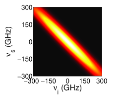
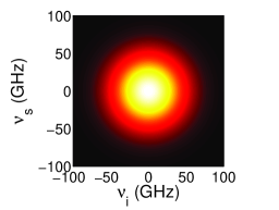
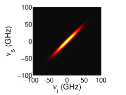
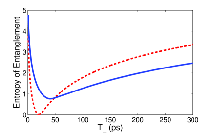
Figure 1: Joint spectrum of the two-photon state for different values of $T_{-}$: (a) $T_{-}=2\;\mbox{ps}$, (b) $T_{-}=20\;\mbox{ps}$, and (c) $T_{-}=200\;\mbox{ps}$. (d) Entropy of entanglement as a function of $T_{-}$ for Gaussian (red dashed line) and sine cardinal (blue solid line) shapes of the mode function. In all cases, the pump pulse duration is: $T_{+}=10\;\mbox{ps}$.

The frequency correlations of the down-converted photons can be tuned by carefully selecting the values of $T_{+}$ and $T_{-}$. Figures 1(a) to 1(c) show the joint probability distribution of the two-photon state $S\left(\nu_{s},\nu_{i}\right)=\left|\Phi\left(\nu_{s},\nu_{i}\right)\right|^{2}$, which measures the probability of detecting a signal photon of frequency $\omega_{s}^{0}+\nu_{s}$ in coincidence with an idler photon of frequency $\omega_{i}^{0}+\nu_{i}$. Frequency anti-correlated photons [Fig. 1(a)] ($\nu_{s}\sim-\nu_{i}$) are obtained when $T_{+}\gg T_{-}$, whereas for $T_{+}\ll T_{-}$, we obtain frequency correlated photons [Fig. 1(c)]. In the particular case when $T_{-}=2T_{+}$, frequency uncorrelated pairs of photons [Fig. 1(b)] are generated. Figure 1(d) (red dashed line) shows the dependence of the entropy of entanglement with $T_{-}$ for a fixed value of $T_{+}$, for a mode function of the form given by Eq. (17).

Using the initial two-photon state described by Eq. (17), we find that the TPA transition probability is given by

$$P_{g\rightarrow f}\left(T_{-},T_{+};\tau\right)= \frac{32\pi\omega_{0}^{2}}{\hbar^{2}\epsilon_{0}^{2}c^{2}A^{2}}T_{+}T_{-}\exp\left[-2T_{+}^{2}\left(\varepsilon_{g}-\varepsilon_{f}+\omega_{p}\right)^{2}\right]$$ (18)

$$\times\left|\sum_{j}D^{\left(j\right)}\left\{F_{+}\left[\eta^{\left(j\right)}T_{-};\tau\right]\exp\left[-i\eta^{\left(j\right)}\tau\right]\right.\right.$$

$$\left.{\color[rgb]{1,1,1}\sum_{j}}\left.+F_{-}\left[\eta^{\left(j\right)}T_{-};\tau\right]\exp\left[i\eta^{\left(j\right)}\tau\right]\right\}\right|^{2},$$

where $\eta^{\left(j\right)}=\Delta^{\left(j\right)}-i\kappa_{j}/2$, with the energy mismatch given by $\Delta^{\left(j\right)}=\varepsilon_{j}-\varepsilon_{g}-\omega_{0}$, and the function $F$ defined as

$$F_{\pm}\left(\xi;\tau\right)=\exp\left(-\xi^{2}\right)\left[1-\frac{2i}{\sqrt{\pi}}\int_{0}^{\xi\pm\frac{i\tau}{2T_{-}}}\exp\left(y^{2}\right)dy\right].$$ (19)

We have computed the TPA transition probability as a function of the delay between photons considering states bearing different types of correlations, particularly for uncorrelated and anti-correlated pairs of photons. As previously obtained, in the case of uncorrelated photons, the TPA signal is constant with the delay $\tau$, so no spectroscopic information about intermediate levels is available.

Surprisingly, in the case of anti-correlated photons, the TPA transition probability is also constant with the delay $\tau$, which means that information about the energy level structure of the medium cannot be retrieved from the TPA signal either. This result is of great interest since it tells us that the use of a source of paired photons with entanglement does not guarantee the successful retrieval of such information. We need to consider another property of the two-photon state that is needed in order to perform virtual-state spectroscopy, namely a specific spectral shape of the frequency correlations.

3.3.2 Two-photon state with a Sine cardinal spectral shape

Fortunately, two-photon states with a Gaussian shape, which require a strong filtering of the pair of photons [36], are not naturally harvested in SPDC. By considering a more realistic shape of the mode function, we will show that two-photon virtual-state spectroscopy can retrieve the sought-after information about the energy level structure under a great variety of circumstances.

As in the previous section, we consider a type-II SPDC process where an additional nonlinear crystal of length $L/2$ is used to achieve group velocity compensation. By introducing a tunable delay $\tau$ between the photons, without restricting their spectrum, the normalized mode function is written as

$$\Phi\left(\nu_{s},\nu_{i}\right)= \left(\frac{T_{-}T_{+}}{2\pi\sqrt{2\pi}}\right)^{1/2}\exp\left[-T_{+}^{2}\left(\nu_{i}+\nu_{s}\right)^{2}\right]\mbox{sinc}\left[T_{-}\left(\nu_{s}-\nu_{i}\right)/2\right]$$ (20)

$$\times\exp\left[iLN_{p}\left(\nu_{s}+\nu_{i}\right)/2+i\nu_{i}\tau\right].$$

The entropy of entanglement of the two-photon state described by Eq. (20) is shown in Fig. 1(d) (blue solid line). Notice that in this case, due to the presence of the sine cardinal function, only quasi-uncorrelated photons can be generated.

We now make use of the initial two-photon state described by the mode function given in Eq. (20) to write the TPA transition probability as

$$P_{g\rightarrow f}\left(T_{-},T_{+};\tau\right)= \frac{64\pi\omega_{0}^{2}}{\hbar^{2}\epsilon_{0}^{2}c^{2}A^{2}T_{-}}\left[\frac{\sqrt{2}T_{+}}{\sqrt{\pi}}\exp\left[-2T_{+}^{2}\left(\varepsilon_{g}-\varepsilon_{f}+\omega_{p}\right)^{2}\right]\right]$$ (21)

$$\times\left|\sum_{j}A^{\left(j\right)}\left\{2-\exp\left[-i\eta^{\left(j\right)}\left(T_{-}-\tau\right)\right]\right.\right.$$

$$\left.{\color[rgb]{1,1,1}\sum_{j}}\left.-\exp\left[-i\eta^{\left(j\right)}\left(T_{-}+\tau\right)\right]\right\}\right|^{2},$$

where $A^{\left(j\right)}=D^{\left(j\right)}/\eta^{\left(j\right)}$.

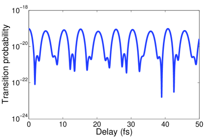
Figure 2: Transition probability as a function of the delay $\tau$ for anti-correlated photons ($T_{-}=2$ ps). Pump pulse duration: $T_{+}=10$ ps. Y-axis in logarithmic scale.

Figure 2 shows the TPA transition probability as a function of the delay between the pulses. Notice the nonmonotonic behavior of the TPA transition probability for anti-correlated photons. This means that spectroscopic information is contained within the TPA signal, which might be related to the energy level structure of the medium. In order to retrieve this information, we follow [7] and perform an average of Eq. (21) over a range of values of $T_{-}$ to obtain the weighted-and-averaged TPA transition probability

$$\bar{P}\left(\tau\right)=\frac{1}{T}\int_{T_{-}^{\mbox{\scriptsize{min}}}}^{T_{-}^{\mbox{\scriptsize{max}}}}P_{g\rightarrow f}\left(T_{-},T_{+};\tau\right)T_{-}dT_{-},$$ (22)

where $T=T_{-}^{\mbox{\scriptsize{max}}}-T_{-}^{\mbox{\scriptsize{min}}}$.

To experimentally perform the average in Eq. (22), a set of experiments with different values of $T_{-}$ are needed. Fortunately, parameter $T_{-}$ can be tuned over a relatively broad range by using different methods, depending on the system configuration. For instance, in type-I SPDC (parallel-polarized photons), changing the width of the pump beam modifies the value of $T_{-}$ [37], whereas in type-II, $T_{-}$ is linearly proportional to the crystal length [38], so a proper set of wedge-shaped nonlinear crystals might be used.

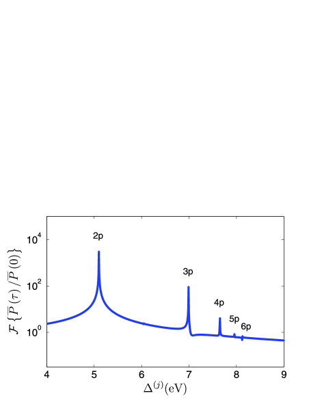
Figure 3: Fourier transform of the normalized weighted-and-averaged TPA transition probability as a function of the energy mismatch $\Delta^{\left(j\right)}$. The delay range considered is $0\leq\tau\leq 2\;\mbox{ps}$, with an integration time of $2\leq T_{-}\leq 10$ ps. Y-axis in logarithmic scale.

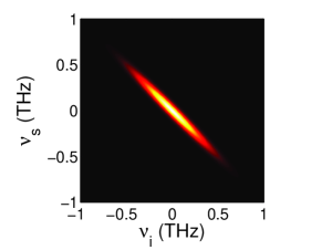
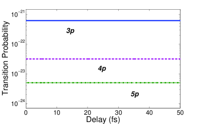
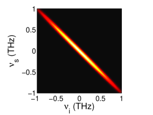
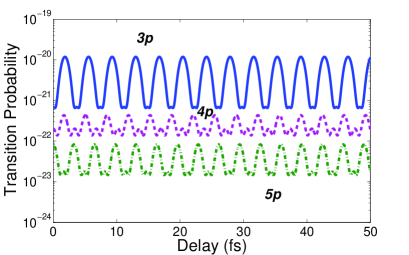
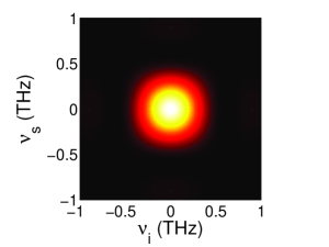
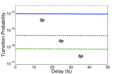
Figure 4: Joint spectrum and single-intermediate level TPA transition probability as a function of the delay $\tau$ for (a,b) Gaussian mode function, (c,d) sine cardinal mode function and (e,f) uncorrelated photons. Intermediate levels correspond to: $3p$ (blue solid line), $4p$ (violet dashed line) and $5p$ (green dash-dotted line). Pump pulse duration is set to $T_{+}=10$ ps and $T_{-}=2$ ps.

Provided that $T\gg 1/\left|\Delta^{\left(j\right)}-\Delta^{\left(k\right)}\right|$, to eliminate unwanted terms at intermediate frequencies, a straightforward Fourier analysis of Eq. (22) reveals the curve shown in Fig. 3. We see that peaks emerge from the Fourier transform of the weighted-and-averaged TPA transition probability, whose locations determine the energy mismatch of the intermediate states: $5.1$, $6.98$, $7.65$, $7.95$, and $8.12$ eV. With these values and the definition of the energy mismatch, we obtain the virtual-state energy values: $-3.40$, $-1.51$, $-0.85$, $-0.54$, and $-0.37$ eV. These energy values can be readily identified with $n=2,3,4,5,6$ corresponding to the $2p$, $3p$, $4p$, $5p$, and $6p$ states, respectively. In obtaining Fig. 3, we have computed the average over $T_{-}$ with a time step $\delta T_{-}=3$ fs. However, one can obtain the same results using a larger time step (up to $60$ fs) to reduce (by an order of magnitude) the amount of experiments that are needed to calculate the weighted-and-averaged TPA transition probability.

To get a clearer picture that two-photon virtual-state spectroscopy depends on the quantum interference from different contributions of intermediate-state transitions with a specific spectral shape, let us consider a simpler, even though ideal, case where a single intermediate quantum state ($3p$, $4p$ or $5p$) is present [36]. Figure 4 shows the two-photon transition probability as a function of the delay $\tau$ for a fixed value of $T_{-}$ and $T_{+}$, considering three different intermediate states. Notice that in the case of an entangled two-photon state bearing a Gaussian mode function [Fig. 4(a,b)], and an uncorrelated two-photon state [Fig. 4(e,f)], contributions from different intermediate transitions are monotonically dependent on the delay $\tau$. In contrast, when considering an entangled two-photon state with a sine cardinal mode function [Fig. 4(c,d)], contributions from different intermediate states exhibit an oscillatory behavior, whose frequency of oscillation corresponds precisely to the frequency of each transition. In consequence, the coherent summation of these contributions [Eq. (21)] leads to nonmonotonic variations in the TPA signal [Fig. (2)] that carry information about the frequency of all intermediate-state transitions. This information can then be extracted by means of a Fourier analysis of the weighted-and-averaged TPA signal [Eq. (22)].

The physical reason why two-photon states with similar degree of entanglement, but different spectral shape, give rise to such contrasting results comes from the fact that TPA probabilities are significantly affected by the shape of the two-photon mode function, as it has been shown, for instance, in Ref. [36]. By increasing the time difference between the absorbed photons, i.e., increasing $T_{-}$ or $\tau$, one would expect a monotonic decay of the TPA signal, which is precisely what is observed with a Gaussian spectral shape. Surprisingly, when considering a sine cardinal spectral shape (rectangular in the time domain), one can find values of $T_{-}$ and $\tau$ where TPA is no longer observed, a phenomenon called entanglement-induced two-photon transparency [6]. In two-photon virtual-state spectroscopy, we benefit from this behavior to extract information about the energy level structure of the medium under study.

It is worth remarking that the particular choice of the pump duration $T_{+}$ does not modify the presented results, since its value does not affect the way in which contributions from different intermediate levels interfere [see Eq. (21)]. Additionally, we highlight the fact that the same information as the one depicted in Fig. 3 can also be obtained when quasi-uncorrelated photons ($T_{-}=40$ ps) are used, meaning that virtual-state spectroscopy can also be performed even with a low degree of entanglement between the photons. This low degree of entanglement, however, results in a lower TPA transition probability [see Eq. (21)], which might affect the signal-to-noise ratio of an experimentally measured TPA signal. This highlights the role of the particular spectral shape of the paired photons used in two-photon virtual-state spectroscopy. While a proper spectral shape of the photons guarantees a successful realization of this technique, the degree of entanglement controls the strength of the TPA signal that is measured.

4 Conclusions

We have shown that virtual-state spectroscopy cannot be performed by means of two uncorrelated rectangular-shaped classical pulses, contrary to what it is suggested in Ref. [24]. Also, we have shown that non-entangled frequency-correlated two-photon states exhibit no dependence of the transition probability on the temporal delay, so they are useless for performing virtual-state spectroscopy. This implies that, in order to extract information about the energy levels of a medium, one has to make use of two-photon states bearing nonclassical frequency correlations. Interestingly, we have found that more important than the degree of entanglement present, it is the specific spectral shape of these correlations which allows one to perform two-photon virtual-state spectroscopy. We have demonstrated that while entangled states with a Gaussian spectral shape and a high degree of entanglement cannot be used to perform virtual-state spectroscopy, surprisingly, entangled two-photon states with a sine cardinal spectral shape and a very low degree of entanglement can be used instead.

The results presented here help to identify clearly which types of two-photon sources can be used to experimentally implement virtual-state spectroscopy. By clarifying the role of entanglement, we have found that even paired photons with a low degree of entanglement, but with the appropriate sine cardinal spectral shape, guarantee the successful realization of virtual-state spectroscopy. This implies that entanglement by itself is not the key ingredient to experimentally perform virtual state spectroscopy.

Finally, this work is also part of a greater research effort devoted to identifying what physical effects necessarily require the presence of entanglement to be observed. Entanglement is a special type of correlation which exists between two parties, i.e., two photons. However, photons can show different types of correlations without entanglement. When a certain effect is observed making use of entangled photons, it might happen that this effect could also have been observed with non-entangled photons, provided that the enabling factor is a specific characteristic of the correlations that is shared between entangled and non-entangled beams of photons. Therefore, it becomes of fundamental relevance to determine whether certain effects are due to the existence of entanglement or to another accompanying characteristic that can exist without its presence.

For instance, in sum-frequency generation (SFG), the flux of generated photons increases with the bandwidth of the incoming fundamental photons [19]. The bandwidth of the absorbed photons can be made extremely large with appropriately engineered SPDC sources [39], which at the same time produces entangled photons with an extremely large degree of entanglement. However, the dependence of the flux rate on the bandwidth applies as well to classical pulses. What it is unique to entangled photons is the linear dependence of the rate on the number of fundamental photons [19]. Paired photons produced in SPDC can also be used to calibrate detectors [40]. In this case, the key enabling factor is the presence of two photons, since SPDC generates necessarily photons in pairs, but not their frequency-entangled nature. When one photon is detected and the other is not, we can infer that this is due to the inefficiency of the detectors. Therefore, by taking the number of photons detected in each detector, and the coincidence counts of paired photons detected in both detectors, we are able to measure the efficiency of each detector. Finally, several protocols proposed for spectroscopy [41] also make use of frequency correlations between photons rather than entanglement. This is closely related to the demonstration of the possibility to use thermal (or pseudothermal), and thus non-entangled, radiation for two-photon imaging experiments [42]. As it was demonstrated in [15], entangled and non-entangled sources can show strikingly similar behaviors when traversing the same optical system, characterized by a particular transfer function, provided that certain properties of the frequency correlations between photons are the same for both sources.

References

References

- [1] Denk W, Strickler J H, and Webb W W 1990 Science 248 73
- [2] Hopfield J J and Worlock J M 1965 Phys. Rev. 137 A1455
- [3] Mukamel S 1995 Principles of Nonlinear Optical Spectroscopy (Oxford University Press, New York)
- [4] Mandel L and Wolf E 1995 Optical Coherence and Quantum Optics (Cambridge University Press, New York)
- [5] Javanainen J and Gould P L 1990 Phys. Rev. A 41 5088
- [6] Fei H -B, Jost B M, Popescu S, Saleh B E A and Teich M C 1997 Phys. Rev. Lett. 78 1679
- [7] Saleh B E A, Jost B M, Fei H -B and Teich M C 1998 Phys. Rev. Lett. 80 3483
- [8] Kojima J and Nguyen Q -V 2004 Chem. Phys. Lett. 396 323
- [9] Schlawin F, Dorfman K, Fingerhut B P and Mukamel S 2012 arXiv:1204.4490v1
- [10] Nasr M B, Saleh B E A, Sergienko A V and Teich M C 2003 Phys. Rev. Lett. 91 083601
- [11] Le Gou t J, Venkatraman D, Wong F N C and Shapiro J H 2010 Opt. Lett. 35 1001
- [12] Franson J D 1992 Phys. Rev. A 45 3126
- [13] Brendel J, Zbinden H and Gisin N 1998 Opt. Comm. 151 35
- [14] Baek S Y, Cho Y W and Kim Y H 2009 Opt. Express 17 19244
- [15] Torres-Company V, Valencia A, Hendrych M and Torres J P 2011 Phys. Rev. A 83 023824
- [16] Torres-Company V, Torres J P and Friberg A T 2012 Phys. Rev. Lett. 109 243905
- [17] Harris S E 2008 Phys. Rev. A 78 021807
- [18] Sensarn S, Yin G Y and Harris S E 2009 Phys. Rev. Lett. 103 163601
- [19] Dayan B, Pe’er A, Friesem A A and Silberberg Y 2005 Phys. Rev. Lett. 94, 043602
- [20] Lee D-I and Goodson III T 2006 J. Phys. Chem. Lett. B 110, 25582
- [21] Lee D-I and Goodson III T 2007 IEEE/LEOS Summer Topical Meetings, 2007 Digest of the, 15-16
- [22] Shore B W 1979 Am. J. Phys. 47 262
- [23] Sakurai J J 1994 Modern Quantum Mechanics (Addison-Wesley, USA)
- [24] Roslyak O and Mukamel S 2009 Phys. Rev. A 79 063409
- [25] Peřina Jr J, Saleh B E A and Teich M C 1998 Phys. Rev. A 57 3972
- [26] Mollow B R 1968 Phys. Rev. 175 1555
- [27] Torres J P, Banaszek K and Walmsley I A 2011 Progress in Optics 56 227
- [28] Law C K, Walmsley I A and Eberly J H 2000 Phys. Rev. Lett. 84 5304
- [29] Etherton R C, Beyer L M, Maddox W E and Bridwell L B 1970 Phys. Rev. A 2 2177
- [30] Cesar C L, Fried D G, Killian T C, Polcyn A D, Sandberg J C, Yu I A, Greytak T J, Kleppner D and Doyle J M 1996 Phys. Rev. Lett. 77 255
- [31] Bethe H A and Salpeter E E 2008 Quantum Mechanics of One- and Two-Electron Atoms (Dover Publications, New York)
- [32] Bebb H B and Gold A 1966 Phys. Rev. 143 1
- [33] The origin of this contradiction lies on the use, in ref. [24], of a wrong identity for multiplication of rectangular functions. This identity creates correlations between the fields, which ultimately lead to a nonmonotonic behavior of the TPA transition probability.
- [34] Keller T E and Rubin M H 1997 Phys. Rev. A 56 1534
- [35] Hendrych M, Micuda M and Torres J P 2007 Opt. lett. 32 2339
- [36] Nakanishi T, Kobayashi H, Sugiyama K and Kitano M 2009 J. Phys. Soc. Jpn. 78 104401
- [37] Joobeur A, Saleh B E A and Teich M C 1994 Phys. Rev. A 50 3349
- [38] Shih Y H and Sergienko A V 1994 Phys. Lett. A 191 201
- [39] Hendrych M, Shi X, Valencia A and Torres J P 2009 Phys. Rev. A 79 023817
- [40] Migdall A L, Datla R U, Sergienko A, Orszak J S and Shih Y H 1995 Metrologia 32 479
- [41] Scarcelli G, Valencia A, Gompers S and Shih Y H 2003 Appl. Phys. Lett. 83 5560
- [42] Valencia A, Scarcelli G, D’Angelo M and Shih Y 2005 Phys. Rev. Lett. 94 063601