Vibrationally Induced Decoherence in Single-Molecule Junctions

Abstract

We investigate the interplay of quantum interference effects and electronic-vibrational coupling in electron transport through single-molecule junctions, employing a nonequilibrium Green’s function approach. Our findings show that inelastic processes lead, in general, to a quenching of quantum interference effects. This quenching is more pronounced for increasing bias voltages and levels of vibrational excitation. As a result of this vibrationally induced decoherence, vibrational signatures in the transport characteristics of a molecular contact may strongly deviate from a simple Franck-Condon picture. This includes signatures in both the resonant and the non-resonant transport regime. Moreover, it is shown that local cooling by electron-hole pair creation processes can influence the transport characteristics profoundly, giving rise to a significant temperature dependence of the electrical current.

I Introduction

In the past decades, electronic components have become continuously smaller and reached the nanoscale. At these scales, electron transport can no longer be understood on purely classical grounds but quantum mechanical effects, such as, for example, the quantization of energy levels, quantum interference effects and tunneling processes need to be taken into account. Single-molecule junctions, where a molecule is contacted by two macroscopic (in most cases, metallic) electrodes, represent prime examples of nanoelectronic devices. These junctions allow to investigate molecules under controllable nonequilibrium conditions and may facilitate an ultimate step in the miniaturization of nanoelectronic devices Nitzan (2001); Galperin et al. (2007a); Cuevas and Scheer (2010); Zimbovskaya and Pederson (2011). It is thus highly desirable to understand the electron transport properties of these junctions.

Experimental studies employing a variety of techniques, such as mechanically controlled break junctions Reed et al. (1997); Reichert et al. (2002); Smit et al. (2002); Böhler et al. (2004); Elbing et al. (2005); Martin et al. (2010); Secker et al. (2011); Ballmann et al. (2010); Kim et al. (2011); Ballmann et al. (2012), scanning tunneling microscopy Stipe et al. (1998); Pascual et al. (2003); Ogawa et al. (2007); Repp et al. (2010); Brumme et al. (2011); Hihath et al. (2010); Arroyo et al. (2010); Cheng et al. (2011); Toher et al. (2011); Heinrich et al. (2011); Fernández-Torrente et al. (2012) and electromigration Sapmaz et al. (2005); de Leon et al. (2008); Hüttel et al. (2009); Osorio et al. (2010), have shown that molecular junctions exhibit a large variety of interesting transport phenomena, including, for example, switching Blum et al. (2005); Lörtscher et al. (2006); Choi et al. (2006); Quek et al. (2009); Wang et al. (2009); Meded et al. (2009); van der Molen and Liljeroth (2010); Mohn et al. (2010), negative differential resistance Pop et al. (2005); Sapmaz et al. (2005); Tal et al. (2008); Osorio et al. (2010); Heinrich et al. (2011), diode- and/or transistor-like behavior Elbing et al. (2005); Yeganeh et al. (2007); Song et al. (2009). Many of these transport properties are not fully understood yet. On one hand, this is due to ambiguities in the contact geometry, which may lead to large variations in the recorded current-voltage characteristics Böhler et al. (2004); Osorio et al. (2007); Hihath et al. (2010); Secker et al. (2011). While strategies to control the contact geometry exist, for example, by the use of special linker groups Hybertsen et al. (2008); Quek et al. (2009), direct binding schemes Kiguchi et al. (2008); Cheng et al. (2011), or click-chemistry approaches Mayor (2009); Chen et al. (2009), the electrodes themselves may show irregular behavior. It is therefore expedient to identify transport properties of molecules that are robust with respect to the contact geometry of the contact, such as, for example, inelastic electron tunneling spectra Stipe et al. (1998); Lorente and Persson (2000); Troisi and Ratner (2006); Galperin et al. (2008a); Dash et al. (2012)). On the other hand, electron transport through a molecular conductor represents a complex many-body problem, where, aside from multiple electronic states, the coupling to numerous vibrational degrees of freedom has to be taken into account Galperin et al. (2007a); Härtle et al. (2009); Secker et al. (2011); Härtle et al. (2011); Ballmann et al. (2012). In contrast to other nanoelectronic devices (e.g. quantum dots Alhassid (2000)), electronic-vibrational coupling is typically rather strong in molecular systems. This is due to their small size and mass and can lead to pronounced vibrational effects in the respective transport characteristics Pascual et al. (2003); de Leon et al. (2008); Ward et al. (2008); Hüttel et al. (2009); Repp et al. (2010); Hihath et al. (2010); Ballmann et al. (2010); Jewell et al. (2010); Osorio et al. (2010); Arroyo et al. (2010); Secker et al. (2011); Kim et al. (2011); Ward et al. (2011); Ballmann et al. (2012). Thereby, the interplay of electronic and the vibrational degrees of freedom of a molecular conductor often involves strong nonequilibrium Härtle et al. (2009); Härtle and Thoss (2011a); Albrecht et al. (2012) as well as quantum mechanical effects Härtle et al. (2011); Ballmann et al. (2012).

A fundamental quantum mechanical effect is quantum interference. The occurrence and observability of quantum interference effects in electron transport through molecular junctions has received great attention recently Härtle et al. (2011); Guedon et al. (2012); Ballmann et al. (2012); van Ruitenbeek (2012). Quantum interference effects in molecular junctions arise because, very similar to a double-slit experiment, an electron may take different pathways through a molecule. Thereby, pathways can be spatially different paths in molecules with an appropriate topology and/or originate from different paths in energy space, e.g., for molecules that exhibit quasidegenerate electronic states Hod et al. (2006); Begemann et al. (2008); Solomon et al. (2008a); Hod et al. (2008); Markussen et al. (2010); Härtle et al. (2011); Ballmann et al. (2012). Recently, strong experimental evidence for quantum interference effects in molecular junctions has been reported Guedon et al. (2012); Ballmann et al. (2012). Moreover, quantum interference effects have been observed in the closely related field of electron transport through quantum dots that are set up as Aharonov-Bohm interferometers Buks et al. (1998); Holleitner et al. (2001); Ihn et al. (2007). Depending on the magnetic flux that is threading the quantum dot, the transmission amplitudes of the electrons interfere constructively or destructively with each other, leading to sizable oscillations in the conductance of such a device Holleitner et al. (2001); Kubala and König (2002); Ihn et al. (2007). A great deal of theoretical work Kalyanaraman and Evans (2002); Collepardo-Guevara et al. (2004); Ernzerhof et al. (2005); Hod et al. (2006); Goyer et al. (2007); Solomon et al. (2008b); Begemann et al. (2008); Darau et al. (2009); Stadler (2009); Brisker-Klaiman and Peskin (2010); Schultz (2010); Markussen et al. (2010); Bergfield et al. (2011); Markussen et al. (2011); Sparks et al. (2011); Brisker-Klaiman and Peskin (2012) has been devoted to study quantum interference effects in molecular junctions, which is, on one hand, due to their fundamental importance but, on the other hand, also due to possible device applications, such as, for example, in transistors Stafford et al. (2007, issued August 31, 2010), thermoelectric devices Bergfield and Stafford (2009); Bergfield et al. (2010) or spin filters Herrmann et al. (2010, 2011). Thereby, in most of the studies, the effect of electron-electron interactions and electronic-vibrational coupling has been neglected.

In this article, we investigate the influence of electronic-vibrational coupling on quantum interference effects in single-molecule junctions. Thereby, we extend our earlier studies Härtle et al. (2011); Ballmann et al. (2012) and analyze in detail the mechanism of vibrationally induced decoherence. Moreover, we consider the effect of local cooling by electron-hole pair creation processes and show how these processes facilitate a mechanism that allows to control quantum interference effects by an external parameter, that is, the temperature of the electrodes. Only recently, this mechanism has been experimentally verified by Ballmann et al. Ballmann et al. (2012) for a number of different junctions, including different molecular species. Note that, in contrast to Refs. Segal et al., 2000; Lehmann et al., 2004; Brisker-Klaiman and Peskin, 2012, we do not consider the vibrational degrees of freedom as being part of a thermal bath but, on the contrary, as active degrees of freedom.

For our studies, we employ a nonequilibrium Green’s function approach developed by Galperin et al. Galperin et al. (2006), which was recently extended by some of us to account for multiple vibrational Härtle et al. (2008) as well as multiple electronic degrees of freedom Härtle et al. (2009, 2010); Volkovich et al. (2011). The approach is based on a separation of electronic and vibrational time scales and, therefore, allows a nonperturbative description of electronic-vibrational coupling as it is required in this nonequilibrium transport problem. Moreover, it suits to describe quasidegenerate levels, which exhibit pronounced quantum interference effects. Besides this approach, a variety of other methods has been developed to describe vibrationally coupled electron transport through nanoelectronic devices. This includes other nonequilibrium Green’s function approaches, which are based on either perturbation theory Mitra et al. (2004); Galperin et al. (2004); Frederiksen et al. (2004); Haupt et al. (2009); Avriller and Levy Yeyati (2009); Schmidt and Komnik (2009); Urban et al. (2010); Entin-Wohlman et al. (2010) or nonperturbative schemes Flensberg (2003); Galperin et al. (2008b); Koch et al. (2010), scattering theory Cizek et al. (2004); Caspary Toroker and Peskin (2007); Zimbovskaya and Kuklja (2009); Jorn and Seidemann (2009), master equation methodologies May (2002); Mitra et al. (2004); Lehmann et al. (2004); Pedersen and Wacker (2005); Reckermann et al. (2008); Leijnse and Wegewijs (2008); Esposito and Galperin (2010); Timm (2011); Dzhioev and Kosov (2012) and a number of numerically exact schemes Han (2006); Eckel et al. (2010); Wang et al. (2011); Albrecht et al. (2012).

The article is organized as follows: In Sec. II.1, we introduce the model Hamiltonian that we use to describe vibrationally coupled electron transport through a single-molecule junction. The nonequilibrium Green’s function approach, which we employ to calculate the corresponding transport characteristics, is outlined in Sec. II.2. In Sec. III.1, we introduce and analyze in detail the basic quantum interference effects that occur in single-molecule junctions. This facilitates the discussion of the effect of vibrationally induced decoherence in the following sections, Secs. III.2 – III.5. Thereby, we study first simplified electronic-vibrational coupling scenarios that allow to investigate basic decoherence phenomena due to vibrations in the resonant (Sec. III.2) and the non-resonant transport regime (Sec. III.3). In addition, we also discuss results for more realistics coupling scenarios. In Secs. III.4 and III.5, we show the importance of cooling by electron-hole pair creation processes in the presence of strong destructive quantum interference effects and how this cooling mechanism can be used to control interference effects by varying the temperature of the electrodes.

II Theory

II.1 Model Hamiltonian

We consider quantum interference effects and vibrationally induced decoherence in electron transport through a single molecule that is bound to two metal leads Galperin et al. (2007a); Cuevas and Scheer (2010); Zimbovskaya and Pederson (2011). This transport problem can be described by a set of discrete electronic states, which are localized on the molecular bridge (M), and a continuum of electronic states, which are localized in the left (L) and the right (R) lead, respectively. Thereby, the states on the molecular bridge are coupled to the states in the leads. The corresponding model Hamiltonian can be written as Härtle and Thoss (2011a)

$$H_{\text{el}} = \sum_{m\in\text{M}}\epsilon_{m}c_{m}^{\dagger}c_{m}+\sum_{m<n\in\text{M}}U_{mn}c_{m}^{\dagger}c_{m}c_{n}^{\dagger}c_{n}+\sum_{k\in\text{L,R}}\epsilon_{k}c_{k}^{\dagger}c_{k}+\sum_{k\in\text{L,R};m\in\text{M}}(V_{mk}c_{k}^{\dagger}c_{m}+\text{h.c.}),\hskip 28.45274pt$$ (1)

where the $\epsilon_{k}$ denote the energies of the lead states and $c_{k}^{\dagger}$ and $c_{k}$ the corresponding creation and annihilation operators. Similarly, the $m$th electronic state on the molecular bridge is addressed by the creation and annihilation operators $c_{m}^{\dagger}$ and $c_{m}$, while its energy is given by $\epsilon_{m}$. Coulomb interactions may give rise to additional charging energies. These energies are accounted for in Hamiltonian (1) by Hubbard-like electron-electron interaction terms, $U_{mn}c_{m}^{\dagger}c_{m}c_{n}^{\dagger}c_{n}$ . In principle, the index $m$ distinguishes different molecular orbitals, including the spin of the electrons. However, as interference effects occur only for transport through orbitals with the same spin, we suppress the spin degree of freedom in the following. The coupling matrix elements $V_{mk}$ in the fourth term of $H_{\text{el}}$ characterize the strength of the interaction between the electronic states of the molecular bridge and the leads and determine the so-called level-width functions $\Gamma_{K,mn}(\epsilon)=2\pi\sum_{k\in K}V_{mk}^{*}V_{nk}\delta(\epsilon-\epsilon_{k})$ ($K$=L,R). Modeling the leads as semi-infinite tight-binding chains with an internal hopping parameter $\gamma=2$ eV, these functions are given by Cizek et al. (2004)

$$\Gamma_{K,mn}(\epsilon) = \frac{\nu_{K,m}\nu_{K,n}}{\gamma^{2}}\sqrt{4\gamma^{2}-(\epsilon-\mu_{K})^{2}},$$ (2)

where, similar to $V_{mk}$, the parameters $\nu_{K,m}$ denote the coupling strength of state $m$ to lead $K$. Thereby, following Refs. Datta et al. (1997); Mujica et al. (2002); Könemann et al. (2006), we assume a symmetric drop of the bias voltage $\Phi$ at the contacts, i.e. the chemical potentials in the left and the right lead are given by $\mu_{\text{L}}=e\Phi/2$ and $\mu_{\text{R}}=-e\Phi/2$, respectively. Note that throughout the paper, the Fermi energy of the leads is set to $\epsilon_{\text{F}}=0$ eV.

Applying a bias voltage an electrical current is flowing through the junction. The molecular bridge may respond to this current, in particular, to the fluctuations of its charge state, which are induced by the tunneling electrons, by adapting its geometrical structure. If the equilibrium positions of the nuclei are different in the different charge states that are probed by the transferred electrons (which is usually the case), transitions between the different vibrational levels become available, and the vibrational degrees of freedom of the junction may be excited according to the standard Franck-Condon picture Koch et al. (2006); Härtle et al. (2008, 2009); Romano et al. (2010); Härtle et al. (2010); Härtle and Thoss (2011a, b); Volkovich et al. (2011). The vibrational degrees of freedom are described in our model as harmonic oscillators that are linearly coupled to the electron densities $c_{m}^{\dagger}c_{m}$ on the molecular bridge Cederbaum and Domcke (1974); Benesch et al. (2008); Han (2010),

$$H_{\text{vib}} = \sum_{\alpha}\Omega_{\alpha}a_{\alpha}^{\dagger}a_{\alpha}+\sum_{m\alpha}\lambda_{m\alpha}Q_{\alpha}c_{m}^{\dagger}c_{m},$$ (3)

where the operator $a^{\dagger}_{\alpha}$ denotes the creation operator of the $\alpha$th oscillator with frequency $\Omega_{\alpha}$ and $Q_{\alpha}=a_{\alpha}+a_{\alpha}^{\dagger}$ the corresponding vibrational displacement operators. The respective coupling strengths are denoted by $\lambda_{m\alpha}$. Finally, the Hamiltonian of the overall system is given by the sum

$$H = H_{\text{el}}+H_{\text{vib}}.$$ (4)

For the nonequilibrium Green’s function approach that we use in this article (cf. Sec. II.2), it is expedient to remove the direct electronic-vibrational coupling term in the Hamiltonian $H$. To this end, we employ the small polaron transformation Mahan (1981); Mitra et al. (2004); Galperin et al. (2006); Härtle et al. (2008)

$$\overline{H} = \text{e}^{S}H\text{e}^{-S}$$

$$= \sum_{m}\overline{\epsilon}_{m}c_{m}^{\dagger}c_{m}+\sum_{m<n}\overline{U}_{mn}c_{m}^{\dagger}c_{m}c^{\dagger}_{n}c_{n}+\sum_{k}\epsilon_{k}c_{k}^{\dagger}c_{k}+\sum_{km}(V_{mk}X_{m}c_{k}^{\dagger}c_{m}+\text{h.c.})+\sum_{\alpha}\Omega_{\alpha}a^{\dagger}_{\alpha}a_{\alpha},$$

with

$$S = -i\sum_{m\alpha}\frac{\lambda_{m\alpha}}{\Omega_{\alpha}}c^{\dagger}_{m}c_{m}P_{\alpha},$$ (6)

$$X_{m} = \text{exp}[i\sum_{\alpha}\frac{\lambda_{m\alpha}}{\Omega_{\alpha}}P_{\alpha}],$$ (7)

and $P_{\alpha}=-i(a_{\alpha}-a_{\alpha}^{\dagger})$ the momentum operator associated with vibrational mode $\alpha$. Note that, although there is no explicit electronic-vibrational coupling in $\overline{H}$, it appears in the transformed Hamiltonian $\overline{H}$ at three different places: $i$) in the polaron-shifted energies ${\overline{\epsilon}_{m}=\epsilon_{m}-\sum_{\alpha}(\lambda_{m\alpha}^{2}/\Omega_{\alpha})}$, $ii$) in additional electron-electron interactions, which add to the original electron-electron interaction terms ${\overline{U}_{mn}=U_{mn}-2\sum_{\alpha}(\lambda_{m\alpha}\lambda_{n\alpha}/\Omega_{\alpha})}$ and $iii$) in the molecule-lead coupling term $\sum_{km}(V_{mk}X_{m}c_{k}^{\dagger}c_{m}+\text{h.c.})$, which is renormalized by the shift operators $X_{m}$.

Because we focus in this article on the effect of electronic-vibrational coupling on the transport characteristics of a single-molecule junction, we suppress the effect of electron-electron interactions in the following, that is we set the renormalized electron-electron interaction strengths $\overline{U}_{mn}$ to zero. A discussion of the effect of electron-electron interactions on the transport characteristics of a molecular junction can be found, for example, in our earlier work, Refs. Härtle et al., 2009; Härtle and Thoss, 2011a; Volkovich et al., 2011, or in Refs. Fransson, 2005; Paaske and Flensberg, 2005; Sela et al., 2006; Galperin et al., 2007b; Han, 2010; Segal et al., 2011. In this context, it is interesting to note that for high bias voltage and within the wide-band approximation, electron-electron interactions have no substantial influence on the electrical current. This was shown by Gurvitz and Prager Gurvitz and Prager (1996); Gurvitz (1998) based on their exact microscopic rate equation methodology. At small (finite) bias voltages, however, it has already been demonstrated that in the presence of electron-electron interactions quantum interference effects become quenched by spin-flip processes König and Gefen (2001); Aikawa et al. (2004); König and Gefen (2002); Ihn et al. (2007). We like to stress that these effects are interesting on their own and very important, but that they are beyond the scope of this work.

II.2 Nonequilibrium Green’s function approach

The central quantities in (nonequilibrium) Green’s function theory are the single-particle Green’s functions, which are given for the electronic degrees of freedom by

$$G_{mn}(\tau,\tau^{\prime}) = -i\langle\text{T}_{c}c_{m}(\tau)c_{n}^{\dagger}(\tau^{\prime})\rangle_{H}.$$ (8)

They allow to calculate all single-particle observables, such as, e.g., the population of levels or the current flowing through the junction. We employ the following ansatz to calculate these Green’s functions Galperin et al. (2006):

$$G_{mn}(\tau,\tau^{\prime}) = -i\langle\text{T}_{c}c_{m}(\tau)c_{n}^{\dagger}(\tau^{\prime})\rangle_{H}\,=\,-i\langle\text{T}_{c}c_{m}(\tau)X_{m}(\tau)c_{n}^{\dagger}(\tau^{\prime})X^{\dagger}_{n}(\tau^{\prime})\rangle_{\overline{H}}$$

$$\approx \bar{G}_{mn}(\tau,\tau^{\prime})\langle\text{T}_{c}X_{m}(\tau)X_{n}^{\dagger}(\tau^{\prime})\rangle_{\overline{H}},\qquad$$

with the electronic Green’s functions $\bar{G}_{mn}(\tau,\tau^{\prime})=-i\langle\text{T}_{c}c_{m}(\tau)c_{n}^{\dagger}(\tau^{\prime})\rangle_{\overline{H}}$ and $\text{T}_{c}$ the time-ordering operator on the Keldysh contour. Thereby, the indices $H/\overline{H}$ indicate the Hamiltonian that is used to evaluate the respective expectation values. The effective factorization of the single-particle Green’s functions $G_{mn}$ into a product of the electronic Green’s functions, $\bar{G}_{mn}$, and a correlation function of shift operators, $\langle\text{T}_{c}X_{m}(\tau)X_{n}^{\dagger}(\tau^{\prime})\rangle_{\overline{H}}$, is justified, if the dynamics of the electronic and the vibrational degrees of freedom take place on different time scales. This is conceptually similar to the Born-Oppenheimer approximation Born and Oppenheimer (1927); Domcke et al. (2004). In the present context, however, we do not address the adiabatic regime, where the Born-Oppenheimer approximation applies, but rather the opposite regime, that is the anti-adiabatic regime, where the time scales for electron tunneling events are much longer than the ones for vibrational motion such that the nuclei of the molecule can follow the corresponding charge fluctuations.

Employing the equations of motion for the electronic Green’s functions $\bar{G}_{mn}$,

$$(i\partial_{\tau}-\bar{\epsilon}_{m})\bar{G}_{mn}(\tau,\tau^{\prime})(-i\partial_{\tau^{\prime}}-\bar{\epsilon}_{n}) = \delta(\tau,\tau^{\prime})(-i\partial_{\tau^{\prime}}-\bar{\epsilon}_{n})+\Sigma_{\text{L},mn}(\tau,\tau^{\prime})+\Sigma_{\text{R},mn}(\tau,\tau^{\prime}),$$

the respective self-energies due to the coupling of the molecule to the left and the right leads, $\Sigma_{\text{L},mn}(\tau,\tau^{\prime})$ and $\Sigma_{\text{R},mn}(\tau,\tau^{\prime})$, can be obtained. These self-energies are given to second order in the molecule-lead coupling by

$$\Sigma_{\text{L/R},mn}(\tau,\tau^{\prime})=\sum_{k\in\text{L/R}}V_{mk}^{*}V_{nk}g_{k}(\tau,\tau^{\prime})\langle\text{T}_{c}X_{n}(\tau^{\prime})X_{m}^{\dagger}(\tau)\rangle_{\overline{H}},$$ (11)

where $g_{k}(\tau,\tau^{\prime})$ denotes the free Green’s function associated with lead state $k$. The real-time projections of these self-energies determine the electronic part of the single-particle Green’s functions $G_{mn}$. In the energy domain the corresponding Dyson-Keldysh equations read

$$\bar{G}^{\text{r/a}}_{mn}(\epsilon) = \bar{G}^{0,\text{r/a}}_{mn}(\epsilon)+\sum_{op}\bar{G}^{0,\text{r/a}}_{mo}(\epsilon)\left(\Sigma^{\text{r/a}}_{\text{L},op}(\epsilon)+\Sigma^{\text{r/a}}_{\text{R},op}(\epsilon)\right)\bar{G}^{\text{r/a}}_{pn}(\epsilon),$$ (12)

$$\bar{G}^{</>}_{mn}(\epsilon) = \sum_{op}\bar{G}^{\text{r}}_{mo}(\epsilon)\left(\Sigma^{</>}_{\text{L},op}(\epsilon)+\Sigma^{</>}_{\text{R},op}(\epsilon)\right)\bar{G}^{\text{a}}_{pn}(\epsilon),$$ (13)

with

$$\bar{G}^{0,\text{r/a}}_{mn}(\epsilon) = \delta_{mn}\frac{1}{\epsilon-\overline{\epsilon}_{m}+i\eta},$$ (14)

where $\eta$ denotes a positive infinitesimal number. Note that Eqs. (12) and (13) give the exact result in the non-interacting limit, that is for $\lambda_{m\alpha}\rightarrow 0$, as well as for an isolated molecular bridge, where $V_{mk}\rightarrow 0$.

Besides the electronic Green’s functions $\bar{G}_{mn}$, we also need to evaluate the correlation functions of the shift operators, $\langle\text{T}_{c}X_{m}(\tau)X_{n}^{\dagger}(\tau^{\prime})\rangle_{\overline{H}}$, in order to obtain the full single-particle Green’s functions $G_{mn}$. To this end, we use a second-order cumulant expansion in the dimensionless coupling parameters $\frac{\lambda_{m\alpha}}{\Omega_{\alpha}}$ Galperin et al. (2006); Härtle et al. (2008, 2010)

$$\langle\text{T}_{c}X_{m}(\tau)X_{n}^{\dagger}(\tau^{\prime})\rangle_{\overline{H}}=\text{exp}\left(\sum_{\alpha\beta}i\frac{\lambda_{m\alpha}\lambda_{n\beta}}{\Omega_{\alpha}\Omega_{\beta}}D_{\alpha\beta}(\tau,\tau^{\prime})-i\frac{\lambda_{m\alpha}\lambda_{m\beta}+\lambda_{n\alpha}\lambda_{n\beta}}{2\Omega_{\alpha}\Omega_{\beta}}D_{\alpha\beta}(\tau,\tau)\right),$$ (15)

with the momentum correlation functions

$$D_{\alpha\beta}=-i\langle\text{T}_{c}P_{\alpha}(\tau)P_{\beta}(\tau^{\prime})\rangle_{\overline{H}}.$$ (16)

Employing the equation of motion for $D_{\alpha\beta}$

$$\frac{1}{4\Omega_{\alpha}\Omega_{\beta}}(-\partial^{2}_{\tau}-\Omega_{\alpha}^{2})D_{\alpha\beta}(\tau,\tau^{\prime})(-\partial^{2}_{\tau^{\prime}}-\Omega_{\beta}^{2}) = \delta(\tau,\tau^{\prime})\delta_{\alpha\beta}(-\partial^{2}_{\tau^{\prime}}-\Omega_{\beta}^{2})\frac{1}{2\Omega_{\beta}}+\Pi_{\text{el},\alpha\beta}(\tau,\tau^{\prime}),$$

we determine the corresponding self-energy matrix $\Pi_{\text{el},\alpha\beta}$. The self-energy matrix $\Pi_{\text{el},\alpha\beta}$, which describes the interactions between the vibrational modes and the electronic degrees of freedom of the molecular bridge, is evaluated up to second order in the molecule-lead coupling Galperin et al. (2006); Härtle et al. (2008, 2010); Volkovich et al. (2011)

$$\Pi_{\text{el},\alpha\beta}(\tau,\tau^{\prime})=-i\sum_{mn}\frac{\lambda_{m\alpha}\lambda_{n\beta}}{\Omega_{\alpha}\Omega_{\beta}}(\Sigma_{mn}(\tau,\tau^{\prime})\bar{G}_{nm}(\tau^{\prime},\tau)+\Sigma_{nm}(\tau^{\prime},\tau)\bar{G}_{mn}(\tau,\tau^{\prime})).$$ (18)

Since $\Pi_{\text{el},\alpha\beta}$ depends on the electronic self-energies $\Sigma_{mn}=\Sigma_{\text{L},mn}+\Sigma_{\text{R},mn}$ and Green’s functions $\bar{G}_{mn}$, Eqs. (11) – (18) constitute a closed set of coupled nonlinear equations that needs to be solved iteratively in terms of a self-consistent scheme Galperin et al. (2006); Härtle et al. (2008).

With the Green’s functions $D_{\alpha\beta}$ and $G_{mn}$, the average vibrational excitation of each vibrational mode is obtained according to Härtle et al. (2008, 2010); Volkovich et al. (2011)

$$\langle a^{\dagger}_{\alpha}a_{\alpha}\rangle_{H} \approx -\frac{1}{2}\text{Im}\left[D^{<}_{\alpha\alpha}(t=0)\right]-\frac{1}{2}+\sum_{m}\frac{\lambda_{m\alpha}^{2}}{\Omega_{\alpha}^{2}}\text{Im}[\bar{G}^{<}_{mm}(t=0)]$$

$$+2\sum_{m<n}\frac{\lambda_{m\alpha}\lambda_{n\alpha}}{\Omega_{\alpha}^{2}}\text{Im}[\bar{G}^{<}_{mm}(t=0)]\text{Im}[\bar{G}^{<}_{nn}(t=0)]$$

$$-2\sum_{m<n}\frac{\lambda_{m\alpha}\lambda_{n\alpha}}{\Omega_{\alpha}^{2}}\text{Im}[\bar{G}^{<}_{mn}(t=0)]\text{Im}[\bar{G}^{<}_{nm}(t=0)],$$

where we use the Hartree-Fock factorization

$$\langle c_{m}^{\dagger}c_{m}c_{n}^{\dagger}c_{n}\rangle_{\overline{H}}\approx\langle c_{m}^{\dagger}c_{m}\rangle\langle c_{n}^{\dagger}c_{n}\rangle-\langle c_{m}^{\dagger}c_{n}\rangle\langle c_{n}^{\dagger}c_{m}\rangle$$ (20)

for $m\neq n$. The current is calculated employing the Meir-Wingreen-like formula Meir and Wingreen (1992); Nitzan (2001); Härtle et al. (2008, 2009)

$$I = 2e\int\frac{\text{d}\epsilon}{2\pi}\,\sum_{mn}\left(\Sigma_{\text{L},mn}^{<}(\epsilon)\bar{G}^{>}_{nm}(\epsilon)-\Sigma_{\text{L},mn}^{>}(\epsilon)\bar{G}^{<}_{nm}(\epsilon)\right).$$ (21)

Note that this expression includes a factor of two to account for spin degeneracy.

III Results

In this section we discuss quantum interference effects and vibrationally induced decoherence in single-molecule junctions based on the methodology introduced above. Thereby, we consider models of increasing complexity. First, in Sec. III.1, we discuss the basic quantum interference effects that occur in electron transport through single molecules. Thereby, we introduce the framework and the methodology that we use to analyze quantum interference effects in general. Next, in Secs. III.2 and III.3, we study the effect of electronic-vibrational coupling on the transport characteristics of a single-molecule contact. Thereby, we use both simplified coupling scenarios, which facilitate the interpretation of the results and provide a first understanding of the effect of vibrationally induced decoherence, and more complex (yet more realistic) scenarios, which, nevertheless, can be understood on the same grounds. Finally, in Secs. III.4 and III.5, we discuss the effect of local cooling due to electron-hole pair creation processes, which, in the presence of strong destructive quantum interference effects, can become dominant (Sec. III.4). As will be shown in Sec. III.5, this results in a strong temperature dependence of the electrical current that cannot be explained in terms of the temperature dependence of the Fermi distribution functions in the leads Nitzan (2001); Selzer et al. (2004); Poot et al. (2006); Choi et al. (2008); Sedghi et al. (2011).

The parameters for all the models employed in this article are summarized in Tab. 1. They have been chosen to represent typical values for molecular junctions and are similar to those employed in a number of first-principles studies of molecular junctions Benesch et al. (2006); Troisi and Ratner (2006); Benesch et al. (2008); Monturet et al. (2010); Arroyo et al. (2010); Bürkle et al. (2012). It should be noted that we consider only models, where the coupling between the molecule and the electrodes is rather weak, i.e., where the effective factorization of the single-particle Green’s functions, Eq. (II.2), is valid. To this end, the coupling parameter $\nu$, which determines the molecule-lead interaction strengths (see Tab. 1), has been chosen as $\nu=0.1$ eV, meeting the condition for the antiadiabatic approximation (II.2): $|\Gamma_{\text{L/R},mn}(\epsilon)|\leq 2\nu^{2}/\gamma\lesssim\Omega_{1}/10\ll\Omega_{1}$.

	model			$\epsilon_{1}$			$\epsilon_{2}$			$U_{12}$			$\nu_{\text{L},1/2}$			$\nu_{\text{R},1}$			$\nu_{\text{R},2}$			$\Omega_{1}$			$\lambda_{11}$			$\lambda_{21}$			$\gamma$
	DES			0.5			0.505			0			$\nu$			$\nu$			-$\nu$			–			–			–			2
	CON			0.5			0.505			0			$\nu$			$\nu$			$\nu$			–			–			–			2
	DESVIB			0.5			0.53			0			$\nu$			$\nu$			-$\nu$			0.1			0			0.05			2
	CONVIB			0.5			0.53			0			$\nu$			$\nu$			$\nu$			0.1			0			0.05			2
	DESVIB2			0.52401			0.53			0.049			$\nu$			$\nu$			-$\nu$			0.1			0.049			0.05			2
	DESCOOL			0.05123			0.05126			0.00248			$\frac{\nu}{10}$			$\frac{\nu}{10}$			-$\frac{\nu}{10}$			0.005			0.00248			0.0025			0.25

Table 1: Parameters for the models of single-molecule junctions that are investigated in this article. All energy values are given in $\mathrm{eV}$. In all models the temperature of the electrodes $T_{\text{L/R}}$ is set to $10$ K. The value of the molecule-lead coupling parameter is $\nu=0.1$ eV.

III.1 Basic Interference Effects

Quantum interference effects can be constructive or destructive, depending on the model, the physical parameters and/or the specific observable. In this section, we study basic interference effects for two different models of single-molecule junctions. The first model exhibits pronounced destructive interference effects in its conduction properties and is referred to as model DES. The second model, CON, shows constructive interference effects. Note that both systems have been extensively studied before Kalyanaraman and Evans (2002); Collepardo-Guevara et al. (2004); Ernzerhof et al. (2005); Hod et al. (2006); Goyer et al. (2007); Solomon et al. (2008b); Begemann et al. (2008); Darau et al. (2009); Stadler (2009); Brisker-Klaiman and Peskin (2010); Schultz (2010); Markussen et al. (2010); Bergfield et al. (2011); Markussen et al. (2011); Sparks et al. (2011); Brisker-Klaiman and Peskin (2012). They are thus very useful to set the stage for the discussion of vibrationally induced decoherence, which is presented in the subsequent sections, Secs. III.2 – III.5. It is also noted that similar models have been used to study interference effects in quantum dot arrays, in particular in the context of Aharonov-Bohm interferometers Kubala and König (2002); Ueda and Eto (2007); Goldstein and Berkovits (2007); Bedkihal and Segal (2012).

Interference effects arise in electron transport through molecular junctions whenever electrons can traverse the junction along different but equivalent pathways. This is the case, for example, if the electrical current of a junction is carried by two quasidegenerate electronic states. The first model system that we study, model DES (see Tab. 1 for a summary of the respective parameters), comprises two electronic states, which are located at $\epsilon_{1}=0.5$ eV and $\epsilon_{2}=0.505$ eV above the Fermi level of the junction. Both of these states are coupled to the left lead with coupling strengths $\nu_{\text{L},1/2}=0.1$ eV and to the right lead with coupling strengths $\nu_{\text{R},1}=0.1$ eV and $\nu_{\text{R},2}=-0.1$ eV, respectively. These coupling strengths, in particular the different sign in the coupling to the right lead, reflect the different spatial symmetry of the two states, which represent symmetric and antisymmetric combinations of localized molecular orbitals (see Figs. 1a and 1b for a graphical representation of the two electronic states and the corresponding localized molecular orbitals). The coupling to the electrodes induces a broadening of the two states of $\approx 20$ meV that exceeds their level spacing $\epsilon_{2}-\epsilon_{1}=5$ meV, i.e. they are quasidegenerate.

(a)	(b)	(c)	(d)

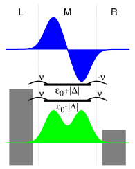
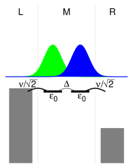
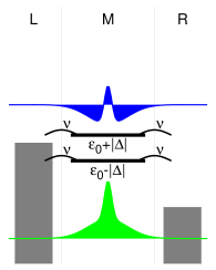
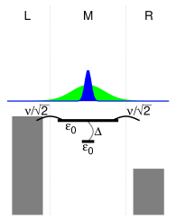
Figure 1: Panel (a): Schematic representation of example wavefunctions of the electronic eigenstates of model DES. Panel (b): Localized molecular orbitals corresponding to the eigenstates of model DES. Panel (c): Schematic representation of example wavefunctions of the electronic eigenstates of model CON. Panel (d): Localized molecular orbitals corresponding to the eigenstates of model CON.

The current-voltage characteristic of junction DES is represented in Fig. 2 by the solid purple line. Due to destructive quantum interference effects, it shows rather low levels of electrical current. This is demonstrated by comparison with the dashed purple line, which depicts the current-voltage characteristic of this junction disregarding quantum interference effects, that is, the incoherent sum of the electrical currents that are flowing through either of the two electronic states. As can be seen, quantum interference effects suppress the current level in this junction by more than an order of magnitude. This applies throughout the whole range of bias voltages considered, including the non-resonant as well as the resonant transport regime, which are separated by the step that appears at $e\Phi\approx 2\epsilon_{1/2}$ in both characteristics.

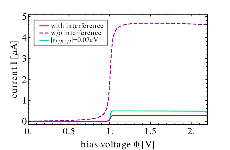
Figure 2: (Color online) Current-voltage characteristics of the linear molecular conductor described by model DES (see Figs. 1a and 1b). The solid purple line depicts the current-voltage characteristic of this junction, including quantum interference effects. The dashed purple line is obtained by discarding them. If the absolute value of the coupling strengths $\nu_{\text{L/R},1/2}$ of model DES is reduced to $0.07$ meV, the current-voltage characteristic depicted by the solid turquoise line is obtained.

Quantum interference effects are destructive in this system, because the outgoing wavefunction, which is associated with an electron tunneling event through state $2$, differs by a phase of $\pi$ from the the one, which is associated with tunneling through state $1$. This is a result of the different spatial structure of the two states and is reflected in the different signs of the respective molecule-lead coupling strengths to the right lead: $\nu_{\text{R},1}=-\nu_{\text{R},2}$. The two outgoing wave functions associated with electron tunneling through state $1$ and $2$, therefore, destructively interfere with each other, leading to a strong suppression of the respective tunnel current. This is illustrated by an example for a resonant and a non-resonant transport process in Figs. 3a and 3b, respectively, where the coherent sum of the outgoing wavefunctions is depicted. Figs. 3c and 3d show the two outgoing wave functions associated with the resonant transport process in Fig. 3a. Note that these interference effects are more pronounced the closer the two electronic states are in energy.

(a)	(b)	(c)	(d)

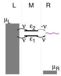
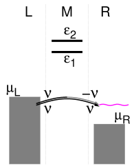
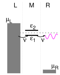
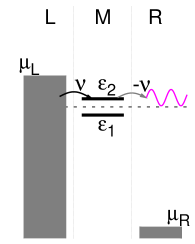
Figure 3: Panel (a) and (b): Resonant and non-resonant electron transport processes through junction DES. The purple wiggly lines depict the coherent sum of the outgoing wavefunctions that are associated with electron tunneling through each of the two electronic states. Panel (c) and (d): Resonant electron transport through state $1$ and $2$ if the other state (i.e. state $2$ and $1$, respectively) would not be present. Due to destructive interference, the corresponding tunneling amplitudes (purple wiggly lines) are much larger than their coherent sum (depicted in Panel (a)).

Employing a different representation, the suppression of the current level in model DES can also be understood on different grounds. Thereby, the two eigenstates of this system are unitarily transformed to two localized states (see Figs. 1a and 1b for a schematic representation of the two equivalent representations). These states have the same energy $\epsilon_{0}$ and are coupled with each other by the coupling strength $\Delta=(\epsilon_{2}-\epsilon_{1})/2$. They represent, for example, the left and the right part of a molecular conductor. Using this local representation, electron transport through this junction involves a sequence of processes: electron transfer from the left electrode to left part of the molecule, followed by an intramolecular electron transfer process from the left part of the molecule to the right part, and finally a transfer process from the right part of the molecule to the right electrode. For $|\nu_{\text{L/R},1/2}|\gtrsim|\Delta|$, the bottleneck for electron transport is the intramolecular electron transfer process. Accordingly, the suppression of the electrical current flowing through junction DES can also be understood in the local representation by the small effective coupling $\Delta$ rather than in terms of quantum interference effects. At high bias voltages, for example, the current flowing through the junction is given by

$$I = 4e\frac{\Gamma}{2}\frac{\left(\frac{\Delta}{\Gamma}\right)^{2}}{\left(\frac{\Delta}{\Gamma}\right)^{2}+1},$$ (22)

according to the exact results derived by Gurvitz and Prager Gurvitz and Prager (1996); Gurvitz (1998), where the wide-band approximation $\Gamma=\Gamma_{\text{L},11}(\mu_{\text{L}})$ is employed. In this expression, $4e\frac{\Gamma}{2}$ represents the current in the limit $\Delta\rightarrow\infty$. The current suppression for finite $\Delta$ is given by the factor $\frac{\left(\frac{\Delta}{\Gamma}\right)^{2}}{\left(\frac{\Delta}{\Gamma}\right)^{2}+1}$. It is solely determined by the ratio $\Delta/\Gamma$. Other aspects of the problem are, however, more straightforwardly understood in the eigenstate representation. For example, if $\Gamma_{\text{L},11}\Gamma_{\text{R},11}\gtrsim\Delta^{2}$, a reduction in the coupling to the leads results in an increase of the current that is flowing through junction DES. This is illustrated by the solid turquoise line in Fig. 2, which shows the current-voltage characteristic of model DES with a reduced coupling to the leads, $\nu_{\text{L},1/2}=\nu_{\text{R},1}=-\nu_{\text{R},2}=0.07$ eV. While this is easily understood in terms of a suppression of destructive interference effects due to a less pronounced broadening of the electronic states, it may hardly be anticipated using the localized state picture, where transport is understood rather as a sequence of intramolecular electron transfer processes.

(a)

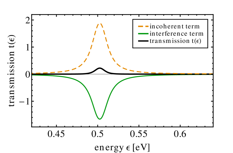
(b)

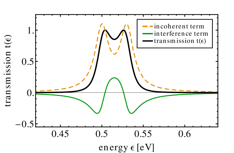
Figure 4: (Color online) Panel (a): The solid black line shows the transmission function of the linear molecular conductor DES (graphically illustrated in Figs. 1a and 1b). In addition, the corresponding incoherent (dashed orange line) and interference term (solid green line) are depicted. Panel (b): The same as Panel (a), where, however, the energy of the second electronic state is shifted from $\epsilon_{2}=0.505$ eV to $\epsilon_{2}=0.53$ eV.

To further analyze quantum interference effects in model DES and to facilitate the discussion of more complex models, we employ the transmission function $t(\epsilon)$ of model DES, which, in general, is defined by Meir and Wingreen (1992); Nitzan (2001)

$$t(\epsilon)=4\pi^{2}\sum_{k\in\text{R},k^{\prime}\in\text{L}}|t_{kk^{\prime}}(\epsilon)|^{2}\delta(\epsilon-\epsilon_{k})\delta(\epsilon-\epsilon_{k^{\prime}})=\sum_{mnop\in\text{M}}\Gamma_{\text{L},mn}(\epsilon)G_{no}^{\text{r}}(\epsilon)\Gamma_{\text{R},op}(\epsilon)G_{pm}^{\text{a}}(\epsilon).$$ (23)

Thereby, $t_{kk^{\prime}}(\epsilon)=\sum_{mn}V_{mk}^{*}G^{\text{r}}_{mn}V_{nk^{\prime}}$ denote the transition matrix elements that represent the transmission amplitudes of the conduction process. Accordingly, the transmission function can be split into an incoherent term

$$t_{\text{inc}}(\epsilon) = 4\pi^{2}\sum_{k\in\text{R},k^{\prime}\in\text{L}}\sum_{mn}|V_{mk}^{*}G^{\text{r}}_{mn}V_{nk^{\prime}}|^{2}\delta(\epsilon-\epsilon_{k})\delta(\epsilon-\epsilon_{k^{\prime}}),$$ (24)

$$= \frac{\Gamma^{2}}{|\epsilon-\epsilon_{1}+i\Gamma|^{2}}+\frac{\Gamma^{2}}{|\epsilon-\epsilon_{2}+i\Gamma|^{2}},$$ (25)

which represents the incoherent sum of the transmission amplitudes $V_{mk}^{*}G^{\text{r}}_{mn}V_{nk^{\prime}}$, and an interference term

$$t_{\text{int}}(\epsilon) = t(\epsilon)-t_{\text{inc}}(\epsilon)\,=\,-2\text{Re}\left[\frac{\Gamma^{2}}{(\epsilon-\epsilon_{1}+i\Gamma)(\epsilon-\epsilon_{2}-i\Gamma)}\right],$$ (26)

which encodes the respective interference effects. The structure of these expressions suggests an equivalent decomposition of the transmission function $t(\epsilon)$ in terms of transmission amplitudes $\Lambda_{1/2}$

$$t(\epsilon) = |\Lambda_{1}-\Lambda_{2}|^{2},$$ (27)

$$t_{\text{inc}}(\epsilon) = |\Lambda_{1}|^{2}+|\Lambda_{2}|^{2},$$ (28)

$$t_{\text{int}}(\epsilon) = \Lambda_{1}^{*}\Lambda_{2}+\Lambda_{2}^{*}\Lambda_{1},$$ (29)

with

$$\Lambda_{1} = \frac{\Gamma}{\epsilon-\epsilon_{1}+i\Gamma},$$ (30a)

$$\Lambda_{2} = \frac{\Gamma}{\epsilon-\epsilon_{2}+i\Gamma}.$$ (30b)

These amplitudes describe electron transport through state $1/2$ if the other state $2/1$ is not present, i.e. in the limit $\epsilon_{2/1}\rightarrow\infty$. It should be noted that the definition of the incoherent term (24) and the interference term (26) is not unique, and depends, for example, on the basis that is used to represent the electronic degrees of freedom of the molecular bridge. Other decomposition schemes, which employ, e.g., molecular conductance orbitals, are possible and have already been used to study interference effects Solomon et al. (2008b). In this work, however, we seek for an understanding of the transport properties of a molecular conductor in terms of its eigenstates, which, in contrast to molecular conductance orbitals, represent an energy-independent basis. For later reference, it is noted that the incoherent term (24) can also be obtained by disregarding the off-diagonal elements of the self-energy matrix $\Sigma^{<,>}_{\text{L}}$ in the current formula (21) (cf. App. A).

Fig. 4a shows the transmission function of junction DES (solid black line) as well as the corresponding incoherent (dashed orange line) and interference term (solid green line). Due to the quasi-degeneracy of the two states, the interference term is almost as large as the incoherent term. It shows only negative values, which indicate destructive interference effects. Thus, the incoherent term, which describes electron transport through this system without quantum interference effects, and the interference term almost cancel each other, leaving only a small peak at $\epsilon\approx(\epsilon_{2}-\epsilon_{1})/2$ in the respective transmission function. This peak is associated with the low current levels that are obtained for this model system (cf. Fig. 2).

Increasing the level spacing in this model by shifting the energy of the second state to higher values, $\epsilon_{2}=0.53$ eV, the tranmission function becomes more complex, as shown in Fig. 4b. The interference term is no longer restricted to negative values, but turns from negative to positive values if the energy of the electron is located between the energy of the first and the second state. Hence, for a larger level spacing, junction DES exhibits both destructive and constructive interference effects. This result is more straightforwardly understood based on the interference picture in the eigenstate representation than in terms of the intramolecular coupling $\Delta$ in the local representation, especially if these constructive interference effects are dominant, such as, for example, if $\epsilon_{1}<\epsilon_{\text{F}}<\epsilon_{2}$.

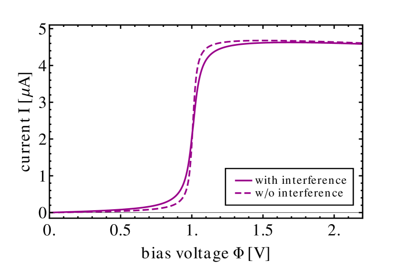
Figure 5: (Color online) Current-voltage characteristics of the branched molecular conductor described by model CON (see Figs. 1c and 1d). The solid purple line depicts the current-voltage characteristic of this junction, including quantum interference effects. The dashed purple line is obtained by discarding them.

Next, we consider model CON. It differs from the previous system only by the sign of the coupling strength $\nu_{\text{R},2}$ (see Tab. 1). The two electronic states of model CON are thus coupled to the right lead by the same coupling strengths ($\nu_{\text{R},1}=\nu_{\text{R},2}$). Due to the different sign, model CON and model DES describe very different types of molecular conductors. While model DES corresponds in the local representation to a linear molecular conductor, model CON describes a branched molecular conductor (cf. Figs. 1c and 1d). Similar to model DES, it can also be unitarily transformed and represented by two localized molecular states that are mutually coupled with each other by the coupling strength $\Delta=(\epsilon_{2}-\epsilon_{1})/2$. While in model DES, however, each of these states is coupled to a different lead, model CON can be mapped onto a delocalized state, which corresponds to the backbone of a molecular conductor that is connected to both electrodes, and a localized state, which corresponds to a side branch of the molecular conductor that is not directly connected to the electrodes of the junction.

The current-voltage characteristic of this junction is represented in Fig. 5 by the solid purple line. In contrast to model DES, it does not show pronounced quantum interference effects. The current flowing through this junction is almost the same as the incoherent sum of the currents that are flowing through each of the two states. This can be inferred by comparison with the dashed purple line, which depicts the respective incoherent sum current. The only difference between these two characteristics is an enhanced broadening of the step that separates the non-resonant and the resonant transport regime at $e\Phi\approx 2\epsilon_{1/2}$.

Figure 6: (Color online) The solid black line shows the transmission function of the branched molecular conductor CON (graphically illustrated in Figs. 1c and 1d). In addition, the corresponding incoherent (dashed orange line) and interference term (solid green line) are depicted.

To understand this result, we analyze the corresponding transmission function. As for model DES (cf. Eqs. 23), it can also be decomposed into an incoherent and an interference term (cf. App. B):

$$t_{\text{inc}}(\epsilon) = |\Lambda_{1}(\epsilon)|^{2}+|\Lambda_{2}(\epsilon)|^{2},$$ (31)

$$t_{\text{int}}(\epsilon) = \Lambda_{1}^{*}(\epsilon)\Lambda_{2}(\epsilon)+\Lambda_{2}^{*}(\epsilon)\Lambda_{1}(\epsilon).$$

with the transmission amplitudes

$$\Lambda_{1} = \frac{\Gamma}{\epsilon-\epsilon_{1}+i\Gamma\frac{2\epsilon-\epsilon_{1}-\epsilon_{2}}{\epsilon-\epsilon_{2}}},$$ (32)

$$\Lambda_{2} = \frac{\Gamma}{\epsilon-\epsilon_{2}+i\Gamma\frac{2\epsilon-\epsilon_{1}-\epsilon_{2}}{\epsilon-\epsilon_{1}}},$$ (33)

which, similar to the amplitudes (30), correctly describe electron transport through junction CON in the two limits $\epsilon_{2/1}\rightarrow\infty$. Fig. 6 depicts the transmission function of this system and the corresponding incoherent and interference term. For low energies $\epsilon<\epsilon_{1}$ as well as high energies $\epsilon>\epsilon_{2}$, constructive interference effects, which are associated with a positive interference term, are indeed active and double the transmittance of the junction. This leads to significantly larger current levels in the non-resonant transport regime, i.e. for $e\Phi<2\epsilon_{1}$ (cf. Fig. 5). For intermediate energies $\epsilon_{1}<\epsilon<\epsilon_{2}$, however, the interference term indicates a transition from constructive to destructive interference effects, similar as for an increased level spacing in model DES (see Fig. 4b). This is accompanied by a steep increase and decrease of the incoherent and the interference term, respectively. At $\epsilon=(\epsilon_{2}+\epsilon_{1})/2$, the two terms are exactly the same and cancel each other. The transmission function of model CON thus drops to zero at this energy, exhibiting an antiresonance. These strong destructive interference effects reduce the increase of the current level at the onset of the resonant transport regime ($e\Phi\approx(\epsilon_{2}+\epsilon_{1})$), leading, in conjunction with the increased current level in the non-resonant transport regime, to a much broader step in the current-voltage characteristic. At higher bias voltages, destructive and constructive interference effects cancel each other such that the same current level is obtained as if interference effects would play no role in this system.

III.2 Vibrationally Induced Decoherence in the Resonant Transport Regime

In this section, we study the influence of electronic-vibrational coupling on the quantum interference effects that we found in the resonant transport regime of model DES and model CON (i.e. for bias voltages $e\Phi\gtrsim 2\epsilon_{1/2}$, cf. Sec. III.1). The influence of this coupling on the corresponding effects in the non-resonant transport regime ($e\Phi<2\epsilon_{1/2}$) are addressed in Sec. III.3.

(a)

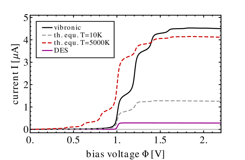
(b)

Figure 7: (Color online) Panel (a): Current-voltage characteristics of the linear molecular conductor DESVIB (solid black line). The dashed gray and red lines depict the current-voltage characteristic of junction DESVIB that is obtained with the vibrational degree of freedom kept in thermal equilibrium at $10$ and $5000$ K, respectively. The solid purple line shows the current-voltage characteristic of model DES. Comparison with this line shows the increase of the current level due to vibrationally induced decoherence in junction DESVIB. Panel (b): Vibrational excitation characteristic corresponding to the vibronic current-voltage characteristic shown in Panel (a).

To study vibrational effects in model DES and model CON, we extend these model systems by coupling to a single vibrational degree of freedom. Thereby, we consider first scenarios, where the vibrational mode is coupled to one of the states only, $\lambda_{11}=0$ eV and $\lambda_{21}=0.05$ eV. The resulting model systems are referred to as model DESVIB and model CONVIB (see Tab. 1 for the complete set of parameters). The specific choice of the electronic-vibrational coupling strengths in these systems is used to simplify the discussion of the corresponding decoherence mechanisms, where, in addition, the energy of the electronic states in models DESVIB and CONVIB have been chosen such that the polaron-shifted levels $\overline{\epsilon}_{m}$ agree with those of models DES and CON. This allows to separate static effects of the vibrations, due to a polaron shift of the energies, from dynamical decoherence effects (vide infra). In addition, we discuss results, where $\lambda_{11}\neq 0$. This may represent more realistic coupling scenarios but, as will be shown, the corresponding decoherence mechanism can be understood on the same grounds as for the simplified coupling scenario. Note that in Ref. Härtle et al. (2011) we have already studied and analyzed the transport characteristics of a single-molecule junction, which is very similar to junction DESVIB.

(a)	(b)	(c)	(d)

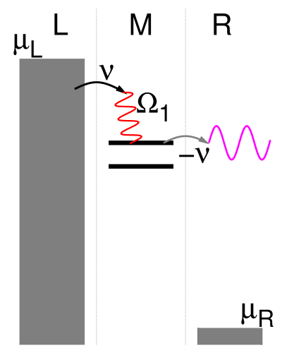
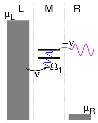
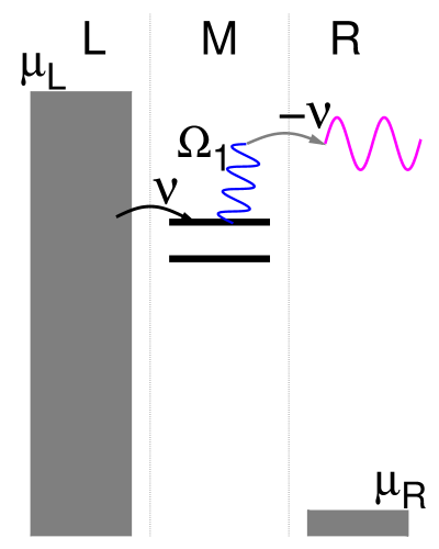
Figure 8: Examples for resonant inelastic electron transport processes, where the vibrational degree of freedom of the junction is singly excited (Panel (a) and (b)) and deexcited (Panel (c) and (d)) upon an electron transfer process from the left electrode onto the molecular bridge (Panel (a) and (c)) or from the molecular bridge to the right lead (Panel (b) and (d)).

The current-voltage characteristic of model DESVIB is represented in Fig. 7a by the solid black line. It is referred to as the vibronic current-voltage characteristic in the following. Similar to the current-voltage characteristic of model DES (solid purple line), it shows a step at $e\Phi=2\overline{\epsilon}_{1/2}$, which indicates the onset of resonant transport processes (cf. Sec. III.1). Besides this step, a number of additional steps can be seen at higher bias voltages, $e\Phi=2(\overline{\epsilon}_{1/2}+n\Omega_{1})$ ($n\in\mathbb{N}$). They correspond to the onset of resonant excitation processes Härtle et al. (2008); Härtle and Thoss (2011a), where electrons tunnel resonantly onto the molecular bridge, exciting the vibrational mode by $n$ vibrational quanta. An example of such an excitation process is graphically depicted in Fig. 8a.

It is also observed that the current level of model DESVIB is much larger than the one of model DES. This is caused by vibrationally induced decoherence that originates from the different vibronic coupling strengths $\lambda_{11}$ and $\lambda_{21}$. Since, in particular, the electronic-vibrational coupling of state $1$ is $\lambda_{11}=0$ eV, electrons traversing the junction can only interact with the vibrational degree of freedom if they pass through state $2$. The interaction with the vibrational mode thus provides ’which-path-information’ that destroys the coherence of the electrons Härtle et al. (2011). Without these decoherence effects, the current levels of model DESVIB would be an order of magnitude smaller and, actually, be the same as for model DES. This is not straightforwardly evident from the corresponding model parameters, since the level spacing in model DESVIB ($\epsilon_{2}-\epsilon_{1}=30$ meV) is larger than in model DES ($\epsilon_{2}-\epsilon_{1}=5$ meV). The polaron-shifted energy levels $\overline{\epsilon}_{1}$ and $\overline{\epsilon}_{2}$ of both model systems, however, are the same. As these are the relevant energies for electron tunneling, destructive quantum interference effects should be as pronounced in model DESVIB as in model DES. As this is not the case and the current level of model DESVIB even reaches the same values as the incoherent sum current of model DES (solid purple line in Fig. 2) at higher bias voltages ($\Phi\gtrsim 1.5$ V), we conclude that in model DESVIB electronic-vibrational coupling strongly quenches destructive quantum interference effects and that this quenching becomes stronger with increasing bias voltages.

The significantly enhanced electrical current of junction DESVIB is not the only manifestation of vibrationally induced decoherence in this system. Also, the relative step heights in the corresponding current-voltage characteristic are strongly influenced by quantum interference effects and vibrationally induced decoherence. Typically, the relative step heights are correlated with the Franck-Condon matrix elements $F_{0n}=\text{exp}(-\lambda_{21}^{2}/\Omega_{1}^{2})(\lambda_{21}^{2n}/\Omega_{1}^{2n})/n!$. These matrix elements determine the probability for a transition from the vibrational ground state to the $n$th excited state, which, for example, may be part of an inelastic excitation process (Figs. 8a). Indeed, there is no strict one to one correspondence between the step heights and the Franck-Condon factors $F_{0n}$, because other processes, like the ones depicted in Figs. 8b – Fig. 8d, and the respective nonequilibrium excitation of the vibrational mode lead, in general, to a suppression of the current level (see Ref. Härtle and Thoss (2011a)). But the first steps in the vibronic current-voltage characteristic of model DESVIB are, nevertheless, far too low. Instead of a ratio of $1:1.2$ between the first and the second step, as it is expected for transport through a single level Härtle and Thoss (2011a), one observes a ratio of $1:2.2$. The successive steps show a similar behavior. This indicates that at the onset of the resonant transport regime destructive quantum interference effects decrease the current level of this system and that, at higher bias voltages, these effects become gradually suppressed as more inelastic processes become active. This is due to an increase of both the number of active excitation and deexcitation processes (Figs. 8a – 8d), where the latter is particularly enhanced by the corresponding level of vibrational excitation (depicted in Fig. 7b), which increases rapidly with the applied bias voltage in the resonant transport regime.

(a)

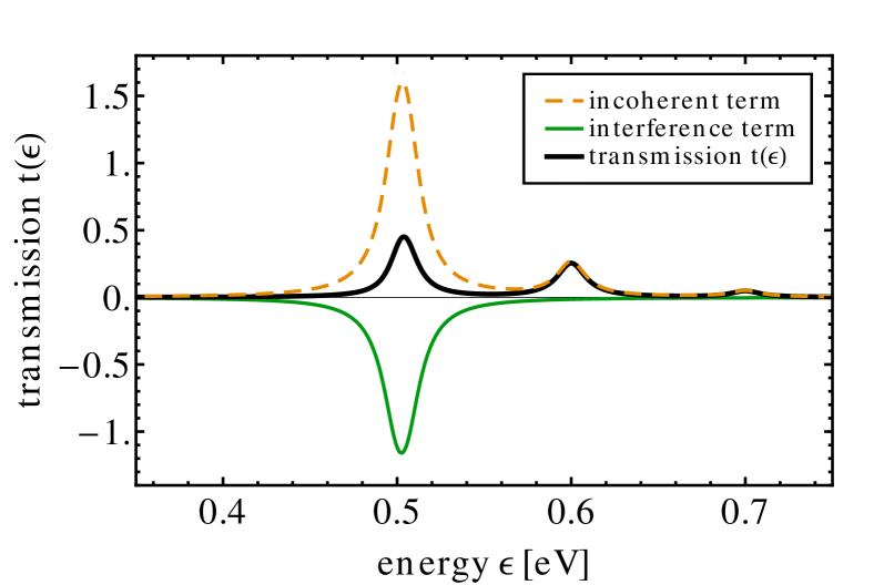
(b)

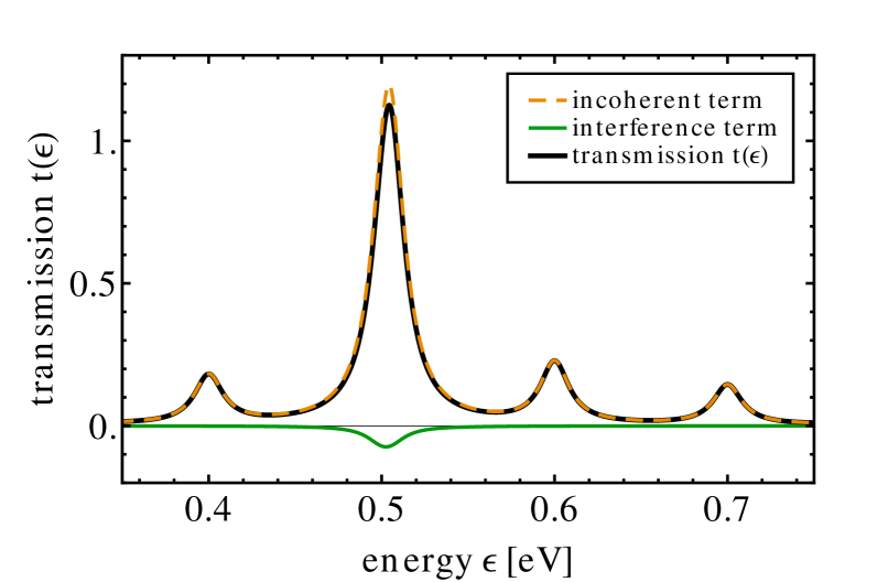
Figure 9: (Color online) Panel (a): The solid black line shows the transmission function of the linear molecular conductor DESVIB for an effective temperature of the vibrational degree of freedom of $10$ K. In addition, the corresponding incoherent (dashed orange lines) and interference terms (solid green lines) are depicted. Panel (b): The same as for Panel (a) but for an effective temperature of the vibrational degree of freedom of $5000$ K.

As before in Sec. III.1, these findings can be analyzed in more detail, considering the transmission function of this system. To define a transmission function in the presence of electronic-vibrational coupling, we restrict the vibrational degree of freedom to its thermal equilibrium state at temperature $T$, employ the wide-band approximation and consider high bias voltages ($e\Phi\gg\epsilon_{1/2}$). With these assumptions, the current through junction DESVIB can be expressed in a form similar to Landauer theory

$$I\approx 2e\int_{-\infty}^{\infty}(\text{d}\epsilon/2\pi)\,t(\epsilon),$$ (34)

with the transmission function

$$t(\epsilon)\equiv i\,\text{tr}\{\mathbf{\Gamma}_{\text{L}}\textbf{G}^{>}\}.$$ (35)

A decomposition of this transmission function in terms of transmission amplitudes is not obvious. Instead, we use the observation (cf. Sec. III.1) that the incoherent term of the transmission function can also be obtained by neglecting the off-diagonal elements of the self-energy matrix in the current formula (21). The interference term is then given by $t_{\text{int}}(\epsilon)=t(\epsilon)-t_{\text{inc}}(\epsilon)$. For our specific model system, we thus obtain (see App. A for details)

$$t_{\text{inc}}(\epsilon) = \frac{\Gamma^{2}}{\left|\epsilon-\overline{\epsilon}_{1}+i\Gamma\right|^{2}}+A^{2}\sum_{l=-\infty}^{\infty}I_{l}(x)\text{e}^{\beta l\Omega_{1}/2}\frac{\Gamma^{2}}{\left|\epsilon-\overline{\epsilon}_{2}-l\Omega_{1}+i\Gamma\right|^{2}},$$ (36a)

$$t_{\text{int}}(\epsilon) = -2A^{2}\Gamma^{2}\text{Re}\left[\frac{1}{(\epsilon-\overline{\epsilon}_{2}+i\Gamma)(\epsilon-\overline{\epsilon}_{1}-i\Gamma)}\right].$$ (36b)

Thereby, the prefactor $A=\text{e}^{-(\lambda_{21}^{2}/(2\Omega_{1}^{2}))(2N_{\text{vib}}+1)}$ is determined by the average vibrational excitation $N_{\text{vib}}=(\text{e}^{\beta\Omega_{1}}-1)^{-1}$ and the inverse temperature $\beta=(k_{\text{B}}T)^{-1}$, while $I_{l}(x)=I_{l}(2(\lambda_{21}^{2}/\Omega_{1}^{2})\sqrt{N_{\text{vib}}(N_{\text{vib}}+1)})$ denotes the $l$th modified Bessel function of the first kind.

The transmission function of model DESVIB, which is obtained according to this scheme, is depicted in Fig. 9 by the solid black line. The corresponding incoherent and interference terms are given by the dashed orange and solid green line, respectively. Thereby, two scenarios are distinguished: (i) the effective temperature of the vibrational degree of freedom is assumed to be $10$ K, i.e. it is effectively not excited, and (ii) the temperature is assumed to be $5000$ K, which results in a level of vibrational excitation that is comparable to the one obtained in the resonant transport regime (cf. Fig. 7b). In both cases, the interference term is significantly weaker with respect to the incoherent term than in the respective electronic transport scenario, which, due to the polaron shift of the electronic energy levels, is the one of model DES (cf. Fig. 4a). Accordingly, the transmittance of the junction is also larger and the corresponding current levels are higher. This can bee seen in Fig. 7a by comparison of the dashed gray and red line, which depict the current-voltage characteristic of model DESVIB with the vibrational mode kept in thermal equilibrium at $10$ and $5000$ K, respectively, with the solid purple line, which depicts the current-voltage characteristic of model DES.

The suppression of the interference term indicates a strong quenching of quantum interference effects in this system. This quenching originates from both a static mechanism that constitutes an effective renormalization of the level-width functions $\Gamma_{K,mm}$ and vibrationally induced decoherence. The factor $A^{2}$, which precedes the interference term (36b), includes both of these effects. It describes, on one hand, the suppression of electronic tunneling events (as, e.g., depicted in Fig. 3) due to electronic-vibrational coupling or, equivalently, the decreased overlap between the vibrational states of different charge states of the molecular bridge. At $10$ K, where the vibrational mode is effectively restricted to its ground state, this suppression corresponds to the Franck-Condon matrix element $F_{00}$. On the other hand, the prefactor $A^{2}$ also includes the effect of vibrationally induced decoherence, which originates from inelastic tunneling processes, where electrons tunnel resonantly through the junction at energies $\approx\overline{\epsilon}_{1/2}$. Examples for such processes are depicted in Figs. 8b and 8d. Inelastic processes, where electrons tunnel resonantly through the junction at energies $\epsilon\approx\overline{\epsilon}_{2}+n\Omega_{1}$ with $n\in\mathbb{Z}/{\{0\}}$ (see Figs. 8a and 8c), complement the effect of vibrationally induced decoherence and result in additional side peaks in the transmission function and the incoherent term but not in the interference term. Both the suppression of the interference term by the prefactor $A^{2}$ and the vibrational side peaks become stronger at higher levels of vibrational excitation, which increases the probability for inelastic processes, in particular deexcitation processes. As a result, the main peak in the interference term, which appears at $\epsilon\approx\overline{\epsilon}_{1/2}$ and is clearly visible in the electronic case, is somewhat reduced in the vibronic case with $10$ K and vanishes almost completely in the vibronic case with $5000$ K. Thus, vibrationally induced decoherence leads to a complete suppression of interference effects in this system as the effective temperature of the vibrational mode (or, equivalently, $N_{\text{vib}}$) increases.

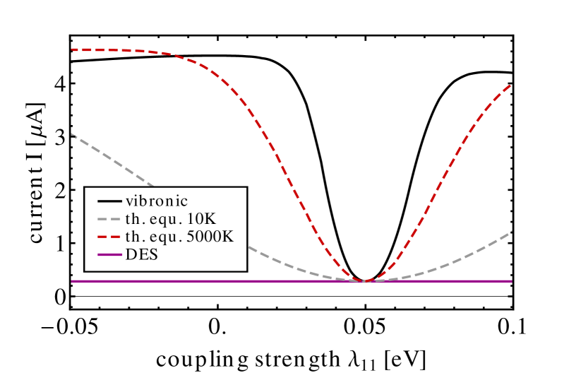
Figure 10: (Color online) Current flowing through junction DESVIB at a bias voltage of $\Phi=2$ V as a function of the electronic-vibrational coupling strength $\lambda_{11}$ (solid black line). All the other parameters of model DESVIB are fixed, in particular, $\lambda_{21}=0.05$ eV. Comparison to the current of model DES (solid purple line) shows that at $\lambda_{11}=\lambda_{21}=0.05$ eV interaction of the tunneling electrons with the vibrations gives no ’which-path’ information and, thus, quantum interference effects suppress the current level of both systems in the same way.

So far, we have restricted our discussion of decoherence effects in model DESVIB to the special scenario, where only one of the electronic states is coupled to the vibrational mode ($\lambda_{11}=0$ while $\lambda_{21}=0.05$ eV$\neq 0$). In most realistic situations both states will be coupled to the vibrational mode. If these couplings are similar, interaction of the tunneling electrons with the vibrational degree of freedom provides less accurate ’which-path’ information and, therefore, the quenching of destructive interference is also less pronounced. This is demonstrated in Fig. 10, where the current level of model DESVIB (at $\Phi=2$ V) is shown as a function of the electronic-vibrational coupling strength $\lambda_{11}$. While vibrationally induced decoherence results in an almost complete suppression of destructive quantum interference effects, if the electronic-vibrational coupling strengths of both states are very different, $|\lambda_{11}-\lambda_{21}|>0.02$ eV, destructive interference effects are active and lead to a strong suppression of the current level, if the coupling strengths of both states are similar, that is for $|\lambda_{11}-\lambda_{21}|<0.01$ eV. The magnitude of the current suppression is thereby determined by the ratio of the electronic parameters $\Delta=\epsilon_{1}-\epsilon_{2}/2$ and $\Gamma$ (as already discussed in Sec. III.1). The corresponding width is, to a large extent, determined by nonequilibrium effects. This can be seen by comparison of the solid black, the dashed gray and the dashed red lines, which correspond to a full nonequilibrium calculation and calculations where the vibrational degree of freedom is restricted to its thermal equilibrium state at $10$ and $5000$ K, respectively. For larger levels of vibrational excitation, the valley of current suppression around $\lambda_{11}\approx\lambda_{21}$ appears to be significantly narrower. This behavior can already be deduced from our analytical result, Eqs. (36). There, the interference term (36b) becomes strongly suppressed, as the prefactor $A$ becomes smaller for larger levels of vibrational excitation $N_{\text{vib}}$. Eqs. (36) also demonstrate that, besides the effective temperature of the vibration, vibrationally induced decoherence is more effective for larger differences of the dimensionless electronic-vibrational coupling strengths $|\lambda_{11}/\Omega_{1}-\lambda_{21}/\Omega_{1}|$. This can be seen by the dashed gray line, where the width of the associated current suppression is given by the frequency of the vibrational mode $\Omega_{1}$.

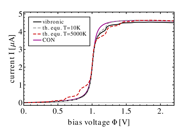
Figure 11: (Color online) Current-voltage characteristics of the branched molecular conductor CONVIB (solid black line). The dashed gray and red lines depict the current-voltage characteristics that are obtained by restricting the vibrational degree of freedom to its thermal equilibrium state at $10$ and $5000$ K, respectively. The solid purple line shows the current-voltage characteristic of model CON.

Next, we consider model CONVIB. The corresponding current-voltage characteristic is shown in Fig. 11. In contrast to model DESVIB, this characteristic does not exhibit pronounced decoherence effects, because in model CON interference effects play, a priori, a less significant role in the resonant transport regime (cf. Sec. III.1). The respective level of vibrational excitation (data not shown) is almost identical to the one of model DESVIB, since inelastic processes, due to the simplified electronic-vibrational coupling scenario ($\lambda_{11}=0$), are not influenced by interference effects in both systems. Analysis of the corresponding transmission function, however, reveals that electronic-vibrational coupling affects quantum interference effects that are active in model CONVIB in a very similar way as in model DESVIB.

Using the same scheme as before, the transmission function and the interference term of model CONVIB are given by (see App. B)

$$t(\epsilon) = c(\epsilon)\left[|\epsilon-\overline{\epsilon}_{2}+i\Gamma|^{2}+2A^{2}(\epsilon-\overline{\epsilon}_{1})(\epsilon-\overline{\epsilon}_{2})-2A^{2}\Gamma^{2}(2-A^{2})\right]$$

$$+A^{2}\sum_{l=-\infty}^{\infty}I_{l}(x)\text{e}^{\beta l\Omega_{1}/2}c(\epsilon-l\Omega_{1})\left(\left|\epsilon-\overline{\epsilon}_{1}-l\Omega_{1}+i\Gamma\right|^{2}-\Gamma^{2}A^{2}\right),$$

$$t_{\text{int}}(\epsilon) = 2A^{2}c(\epsilon)\left[(\epsilon-\overline{\epsilon}_{1})(\epsilon-\overline{\epsilon}_{2})-\Gamma^{2}(1-A^{2})\right],$$ (37b)

with

$$c(\epsilon) = \left|\frac{\Gamma}{(\epsilon-\overline{\epsilon}_{1}+i\Gamma)(\epsilon-\overline{\epsilon}_{2}+i\Gamma)+A^{2}\Gamma^{2}}\right|^{2}.$$ (38)

They are represented in Fig. 12, including the respective incoherent term. Vibrationally induced decoherence causes the same effects as outlined before, that is, a suppression of the interference term and the appearance of side peaks that are not counterbalanced by the interference term. As a result, the antiresonance at $\epsilon=(\overline{\epsilon}_{1}+\overline{\epsilon}_{2})/2$ is quenched and even vanishes as the level of vibrational excitation increases.

(a)

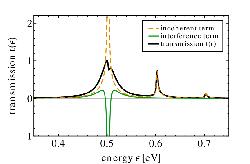
(b)

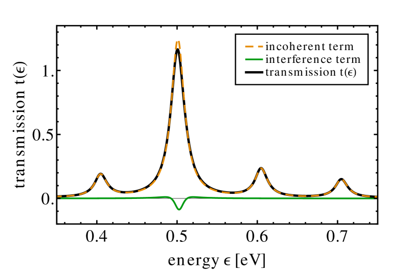
Figure 12: (Color online) Panel (a): The solid black line shows the transmission function of the branched molecular conductor CONVIB for an effective temperature of the vibrational degree of freedom of $10$ K. In addition, the corresponding incoherent (dashed orange lines) and interference terms (solid green lines) are depicted. Panel (b): The same as for Panel (a) but for an effective temperature of the vibrational degree of freedom of $5000$ K.

III.3 Vibrationally Induced Decoherence in the Non-Resonant Transport Regime

While in Sec. III.2 we have focused on the resonant transport regime of a molecular junction, here we investigate the effect of electronic-vibrational coupling on quantum interference effects in the non-resonant transport regime. To this end, we discuss the transport characteristics of the same model systems as in Sec. III.2 but for lower bias voltages: $e\Phi<0.25$ eV$\ll 2\epsilon_{1/2}$.

First, we consider model DESVIB. The corresponding conductance-voltage characteristic (i.e. the differential conductance $\text{d}I/\text{d}\Phi$) is represented by the solid black line in Fig. 13. In the non-resonant transport regime, the conductance of junction DESVIB is almost constant, because the probability of non-resonant transport processes, like the one depicted in Fig. 3b), does not significantly vary with the energy of the tunneling electrons and because the energy window, where these processes can occur, increases linearly with the applied bias voltage. Deviations of this constant behavior arise, whenever the bias voltage exceeds a multiple of the vibrational frequency, $e\Phi\approx n\Omega_{1}$ ($n\in\mathbb{N}$). At these bias voltages steps appear in the conductance-voltage characteristics that are related to the onset of inelastic channels, where electrons are tunneling through the junction non-resonantly by exciting the vibrational degree of freedom (an example process is depicted in Fig. 14a). This behavior is well known and is used, for example, to determine the frequency of vibrational modes in inelastic electron tunneling spectroscopy of molecular junctions Stipe et al. (1998); Lorente and Persson (2000); Troisi and Ratner (2006); Galperin et al. (2008a); Dash et al. (2012).

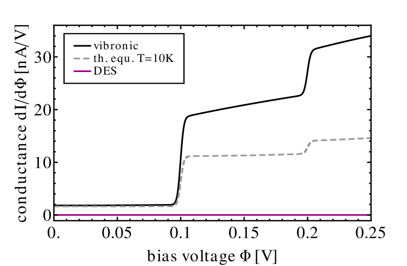
Figure 13: (Color online) Conductance-voltage characteristics of the linear molecular conductor DESVIB (solid black line). The solid purple line shows the conductance-voltage characteristic of junction DES. The dashed gray line depicts the conductance-voltage characteristic of junction DESVIB with the vibrational degree of freedom kept in thermal equilibrium at $10$ K.

(a)	(b)	(c)

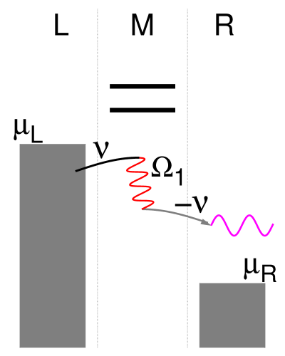
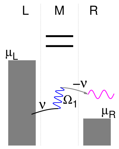
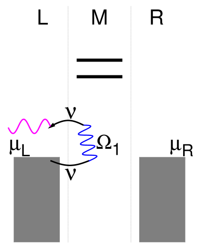
Figure 14: Examples of non-resonant inelastic processes, including transport (Panel (a) and (b)) and electron-hole pair creation processes (Panel (c)). Note that transport processes can occur at low temperatures (i.e. $k_{\text{B}}T_{\text{L/R}}\gg\Omega_{1}$) via the excitation (Panel (a), $e\Phi>\Omega_{1}$) or deexcitation of the vibrational degree of freedom (Panel (b)) while, in contrast, electron-hole pair creation processes involve predominantly deexcitation processes, because the respective excitation processes are suppressed by Pauli blocking.

Vibrationally induced decoherence modifies this picture in a very similar way as in the resonant transport regime. First of all, the current/conductance of junction DESVIB is significantly increased, as is evident by comparison with the conductance-voltage characteristics of junction DES (solid purple line). While, for $e\Phi<\Omega_{1}$, this increase can be solely attributed to the static effect of a decreased overlap between vibrational states of different charge states of the molecular bridge (see Sec. III.2), the opening of inelastic channels at $e\Phi\geq n\Omega_{1}$ leads to vibrationally induced decoherence effects that increase the conductance of junction DESVIB much more. Secondly, the relative step heights in the conductance-voltage characteristics, which should be correlated, in a similar way as the steps in the current-voltage characteristics, with the Franck-Condon matrix elements $F_{0n}$, appear far too large. This is again due to destructive quantum interference effects that suppress the current level at low bias voltages but become less effective the more inelastic processes become active. Thus, for example, the conductance ratio before and after the first step is roughly $1:10$ and not $1:1.3$, as for a comparable scenario with a single electronic state Härtle et al. (2008). Moreover, the conductance of junction DESVIB is not a constant after the onset of the first inelastic channel at $e\Phi=\Omega_{1}$. This is shown by the solid black and the dashed gray line, where nonequilibrium effects or the heating of the vibrational degree of freedom is taken into account and discarded, respectively. As non-resonant excitation processes (an example of which is depicted in Fig. 14a) become availabe for $e\Phi>\Omega_{1}$ and lead to a step-wise increase of the conductance, which is seen in both the black and the gray line, they also result in a finite level of vibrational excitation. Consequently, non-resonant deexcitation processes (Fig. 14b) occur and increase the conductance of the junction even further (which is only visible in the black line). As the number of excitation processes increases continuously for $e\Phi>\Omega_{1}$, the level of vibrational excitation also increases continuously and so does the current contribution of these non-resonant deexcitation processes.

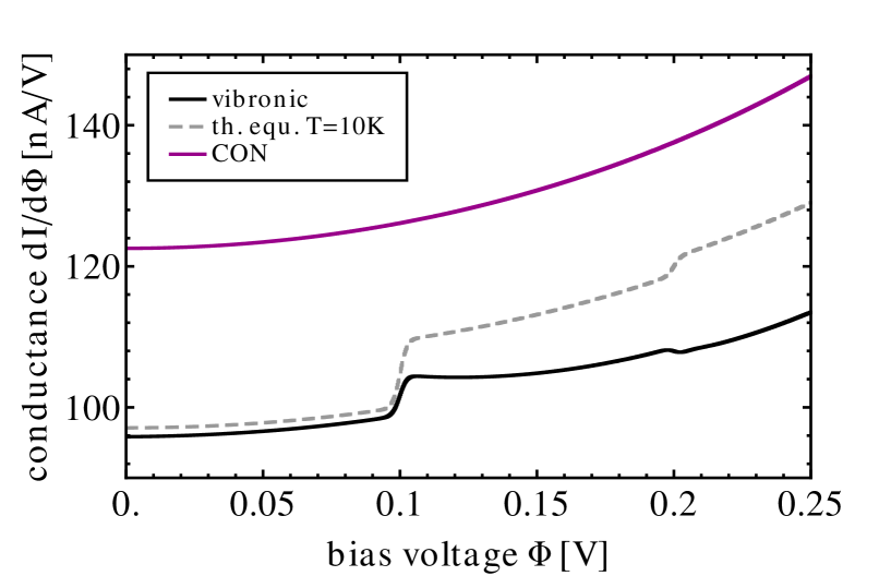
Figure 15: (Color online) Conductance-voltage characteristics of the branched molecular conductor CONVIB. The solid purple line shows the conductance-voltage characteristic of junction CON. The dashed gray line depicts the conductance-voltage characteristic of junction CONVIB, which is obtained by evaluating the vibrational degree of freedom by the thermal equilibrium state that it would acquire at $10$ K.

Next, we investigate non-resonant transport through model CONVIB. The corresponding conductance-voltage characteristics is depicted in Fig. 15. In contrast to junction DESVIB, the vibronic conductance-voltage characteristic exhibits overall smaller conductance values. This is due to both a reduction of the probability for electronic transfer events (Fig. 3b) as well as vibrationally induced decoherence, which quenches the constructive interference effects that are active in this system. Thereby, a higher level of vibrational excitation, due to a more important role of deexcitation processes, leads to a further reduction of conductance (compare the solid black and the dashed gray line). The steps, which appear very pronounced in the vibronic conductance-voltage characteristic of model DESVIB at $e\Phi\backsimeq n\Omega_{1}$ ($n\in\mathbb{N}$), are, therefore, substantially reduced. This reflects the competition between a reduction of conductance due to vibrationally induced decoherence and the increase of conductance due to the onset of non-resonant excitation processes.

Another effect of vibrationally induced decoherence is that the slope of the vibronic conductance-voltage characteristic can even be negative after the onset of an inelastic channel at $e\Phi\approx n\Omega_{1}$ ($n\in\mathbb{N}$). This can be seen, for example, after the first step in the solid black line of Fig. 15 and is related to the number of inelastic processes, which increases with the applied bias voltage $\Phi$. Recall that, for the same reasons, the slope of the conductance-voltage characteristic of junction DESVIB is positive at these bias voltages. In addition, at the opening of the second inelastic channel, $e\Phi\approx 2\Omega_{1}$, the reduction of conductance due to vibrationally induced decoherence may also prevail over the increase of conductance due to the onset of non-resonant excitation processes. This leads to a drop in the conductance of junction CONVIB at these bias voltages. It should be noted that such a decrease of conductance (due to the opening of inelastic transport channels) has been reported before Lorente and Persson (2000); Haupt et al. (2009); Avriller and Levy Yeyati (2009); Schmidt and Komnik (2009) but only for highly conducting molecular junctions ($\text{d}I/\text{d}\Phi\gtrsim 20$ $\mu$A/V). We thus conclude that quantum interference effects and vibrationally induced decoherence have a strong impact on the inelastic tunneling spectra of a molecular junction.

Note that antiresonances such as they appear in model CON have been studied extensively before and have already been considered in the context of molecular spintronics Herrmann et al. (2010, 2011) or thermoelectric devices Bergfield and Stafford (2009); Bergfield et al. (2010). Thereby, it is desirable that the antiresonance is located near the Fermi energy of the junction. Our results suggest that vibrationally induced decoherence puts a strong constraint on these applications. As dynamical excitation and deexcitation processes are weakening such antiresonances in both the resonant and the non-resonant transport regime, they should be located in a rather narrow range of energies around the Fermi energy of the junction, $[\epsilon_{\text{F}}-\Omega_{\text{low}},\epsilon_{\text{F}}+\Omega_{\text{low}}]$, which is determined by the frequency $\Omega_{\text{low}}$ of the low-frequency modes of the respective system.

III.4 Suppression of Local Heating by Destructive Quantum Interference Effects

In Secs. III.1–III.3, we have shown that destructive interference effects suppress the electrical current flowing through a molecular conductor. In this section, we demonstrate that the respective level of vibrational excitation may also be strongly suppressed, in particular in the resonant transport regime, where the level of current-induced vibrational excitation can be very high (cf. Figs. 7b or, e.g., Refs. Koch et al., 2006; Härtle et al., 2008, 2009; Romano et al., 2010; Härtle et al., 2010, 2010; Volkovich et al., 2011; Kast et al., 2011).

To understand the vibrational excitation characteristics of a molecular conductor, in general, one has to take into account excitation and deexcitation processes due to electron transport (cf. Figs. 8a – 8d for resonant transport processes and Figs. 14a – 14b for non-resonant transport processes) but also deexcitation processes, which are associated with electron-hole pair creation processes in the leads . Examples for such electron-hole pair creation processes are depicted in Fig. 14c and Fig. 16, where non-resonant and resonant pair creation processes are shown, respectively. In the course of a pair creation process, an electron is not transferred from one electrode to the other, as in corresponding transport processes, but transfers onto the molecular bridge and, from there, back to the electrode where it came from. Although these processes do not directly contribute to the electrical current that is flowing through the junction, they represent a very important cooling mechanism for the vibrational degrees of freedom Härtle et al. (2010); Härtle and Thoss (2011a, b); Volkovich et al. (2011). Therefore, as the efficiency of transport processes is, inter alia, determined by the level of vibrational excitation, they also have an indirect influence on the electrical transport properties of a molecular conductor. As we have already outlined in Ref. Härtle and Thoss (2011a), this influence can, nonetheless, be substantial.

(a)	(b)

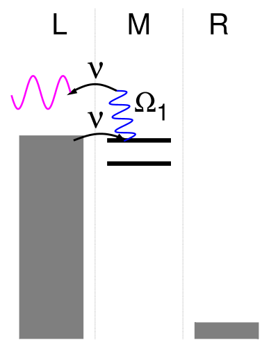
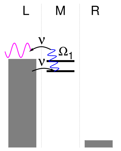
Figure 16: Examples of resonant electron-hole pair creation processes. In contrast to transport processes, which involve both electrodes, these processes involve just one of the leads. They are thus not subject to the destructive quantum interference effects that are active in model DESVIB and, consequently, if destructive interference effects are very pronounced, lead to a strong suppression of the current-induced level of vibrational excitation in such a system (which originates, e.g., from the resonant excitation processes depicted in Figs. 8a and 8b).

In the present context, it is important to note that in model DESVIB inelastic transport processes are not suppressed by destructive quantum interference effects due to the specific electronic-vibrational coupling scenario in this junction (i.e. because $\lambda_{11}=0$). Therefore, we consider another model system in this section, model DESVIB2. It is very similar to model DESVIB but, in contrast, includes electronic-vibrational coupling also in state $1$: $\lambda_{11}\approx\lambda_{21}$ but $\lambda_{11}\neq\lambda_{21}$ (see Tab. 1 for a complete list of parameters). As a consequence of the coupling to both states, inelastic transport processes are, similar to electronic transport processes, also suppressed by destructive quantum interference effects. In contrast, however, electron-hole pair creation processes are not suppressed, because they involve the coupling of an electronic state to just one of the electrodes and not to both, and, even if the respective coupling strength is negative, its square is not.

This has a strong impact on the excitation levels of junction DESVIB2. The corresponding vibrational excitation characteristic is shown in Fig. 17 by the solid black line. It exhibits very similar features as the one shown by model DESVIB but approximately only half of the corresponding vibrational excitation levels (cf. Fig. 7b). This is related to the fact that inelastic transport processes are suppressed by destructive quantum interference effects in this system while electron-hole pair creation processes are not. Thus, the ratio between heating and cooling processes, which is typically between 1:2 or 1:1 for resonant electron transport through a single electronic state Härtle and Thoss (2011b), is shifted towards much lower values, resulting in much lower levels of vibrational excitation.

This cooling effect is even more pronounced, if the level spacing between the two electronic states is smaller and, consequently, the suppression of inelastic transport processes is more pronounced. The solid blue and red line in Fig. 17, for example, show the excitation characteristics of model DESVIB2 for smaller splittings of the (polaron-shifted) energy levels. The corresponding excitation levels are substantially smaller. The only major contribution that remains in the limit $\overline{\epsilon}_{2}\rightarrow\overline{\epsilon}_{1}$ is the one due to the formation of a polaronic state, $\sum_{mn}(\lambda_{m1}\lambda_{n1}/\Omega_{1})\langle c_{m}^{\dagger}c_{m}c_{n}^{\dagger}c_{n}\rangle_{\overline{H}}$ (cf. Eq. (II.2)). This, however, is only a static contribution that originates from charging processes and cannot be used in deexcitation processes. In other words, the current-induced excitation of the vibrational mode is almost completely suppressed in this limit.

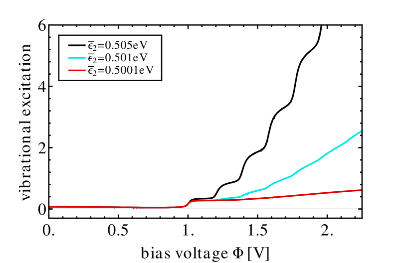
Figure 17: (Color online) Vibrational excitation characteristics of the linear molecular conductor DESVIB2 for different values of the polaron-shifted energy level of state $2$, $\overline{\epsilon}_{2}$.

Having in a mind that states $1$ and $2$ of model DESVIB2 may represent just symmetric and antisymmetric combinations of localized molecular orbitals (see Figs. 1a and 1b), their electronic structure may be very similar and, accordingly, also the respective electronic-vibrational coupling strengths. Indeed, such pairs of electronic states are often found in realistic models of single-molecule junctions Benesch et al. (2006, 2008); Härtle et al. (2011); Ballmann et al. (2012). The cooling mechanism described in this section can, therefore, be expected to occur in a large variety of single-molecule junctions.

III.5 Decoherence-Induced Temperature Dependence of the Current

In Sec. III.4, we have shown that electron-hole pair creation processes facilitate an important cooling mechanism for the vibrational degrees of freedom of a single-molecule contact Härtle et al. (2010); Härtle and Thoss (2011a, b); Volkovich et al. (2011), particularly in the presence of strong destructive quantum interference effects. Within the local representation of the linear molecular conductor by two localized molecular orbitals (as in Fig. 1b), this can be understood in an alternative way: If the intramolecular coupling $\Delta$ becomes very weak, $\Delta\rightarrow 0$, the left and the right part of the molecular conductor decouple. In that sense, the two parts of the molecule behave as being part of the left or right electrode, that is they also acquire the same equilibrium state. This thermalization is facilitated by electron-hole pair creation processes and is comparable to the thermalization of a molecule adsorbed on a surface with the substrate. Thus, the temperature in the electrodes can be used to control the excitation levels of the vibrational modes of the left and the right part of such a molecular conductor. Moreover, as higher levels of vibrational excitation enhance the effect of vibrationally induced decoherence (see Sec. III.2), the temperature in the electrodes can, in turn, be used to control quantum interference effects in single-molecule junctions. This will be demonstrated in this section.

In general, a variation of the temperature of the electrodes is accompanied by a change in the contact geometry of a single-molecule contact, either due to thermal expansion of the electrodes or irreversible drifts of single gold atoms. In experiments, the stability of the contact geometry can often only be maintained for low temperature variations Ballmann et al. (2012). In order to demonstrate control of quantum interference effects via the temperature of the electrodes, we therefore consider a model of a single-molecule contact that includes low-frequency vibrational modes, which, in the given range of temperatures, exhibit significant changes in their excitation levels. To this end, we consider a mode with a frequency of $\Omega_{1}=5$ meV, which represents a frequency value at the lower end of the vibrational spectrum of a larger molecule Benesch et al. (2006, 2008); Härtle et al. (2011). Moreover, we use a range from $10$ K to $100$ K for the temperature of the electrodes in the following, where the corresponding excitation level of the vibrational mode varies between $N_{\text{vib}}=0.003$ and $N_{\text{vib}}=1.3$, respectively. This model system is referred to as model DESCOOL (see Tab. 1 for a complete list of parameters). Besides the low-frequency mode, it includes two electronic states that are almost degenerate, that is $\overline{\epsilon}_{2}-\overline{\epsilon}_{1}\ll\Gamma$.

The current-temperature characteristic of this model system and the corresponding level of vibrational excitation are shown by the solid black lines in Fig. 18. Thereby, we have used a bias voltage of $e\Phi=0.2$ eV$\gg 2\overline{\epsilon}_{1/2}$, which corresponds to the resonant transport regime of this junction. Note that, at this bias voltage, the current level of junction DESCOOL is influenced neither by the thermal broadening of the Fermi distribution functions in the leads Selzer et al. (2004); Poot et al. (2006); Choi et al. (2008); Sedghi et al. (2011) nor vibrational sidepeaks that are associated with the onset of resonant excitation processes (Fig. 8a). As can be seen in Fig. 18, however, the current and the excitation level of the vibrational mode increases substantially with the temperature in the electrodes. We attribute this behavior to the quenching of destructive quantum interference effects by inelastic transport processes, which is enhanced, via the thermalization mechanism described above, for higher temperatures of the electrodes. This shows that the temperature in the electrodes can be used to control destructive quantum interference effects in a single-molecule junction. Note that, very recently, this control mechanism has been demonstrated by Ballmann et al. in mechanically controlled break junction experiments for a variety of different molecules Ballmann et al. (2012).

(a)

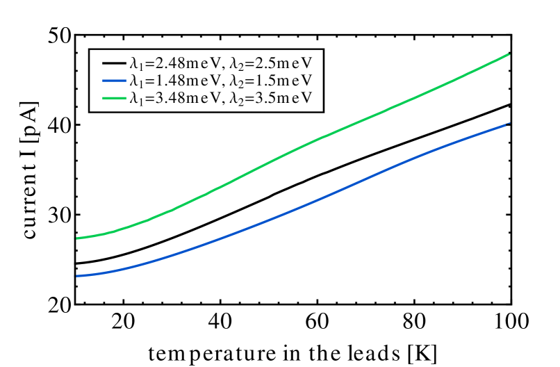
(b)

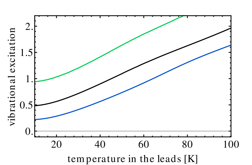
Figure 18: (Color online) Panel (a): Current-temperature characteristics of the linear molecular conductor DESCOOL. Panel (b): Vibrational excitation characteristic corresponding to the current-temperature characteristic shown in Panel (a).

It is interesting at this point to study the temperature dependence of model DESCOOL for different absolute values of the electronic-vibrational coupling strengths $\lambda_{11}$ and $\lambda_{21}$. Thereby, as we have seen in Sec. III.2, it is expedient to keep the difference in the dimensionless couplings constant, i.e. $|\lambda_{11}-\lambda_{21}|/\Omega_{1}$. Accordingly, the solid blue/green lines in Fig. 18 represent the temperature characteristics of model DESCOOL that we obtain by reducing/increasing the two coupling strengths by $1$ meV. These results corroborate that vibrationally induced decoherence is, to a large extent, driven by nonequilibrium effects (see, e.g., the discussion at the end of Sec. III.2), because for smaller electronic-vibrational coupling strengths we find lower levels of vibrational excitation and, due to the consequently less effective quenching of destructive interference effects, a more pronounced suppression of the current level. As a result, the relative temperature dependence $\Delta I=I(100\,\text{K})-I(10\,\text{K})$ is stronger for weaker electronic-vibrational coupling strengths in this system. It should be noted at this point that, in systems where destructive interference effects are not active, weaker electronic-vibrational coupling is typically associated with larger levels of vibrational excitation Härtle and Thoss (2011a). This counterintuitive phenomenon is related to the suppression electron-hole pair creation processes, which, in the resonant transport regime, is more pronounced for higher bias voltages but also for weaker electronic-vibrational coupling. This suppression of pair creation processes is counterbalanced in transport through junction DESCOOL due to the presence of destructive interference effects.

IV Conclusion

We have investigated the role of vibrations in electron transport through single-molecule junctions, which are governed by strong quantum interference effects. To this end, we have employed both analytical and numerical results that are obtained from nonequilibrium Green’s function theory Galperin et al. (2006); Härtle et al. (2008, 2009, 2010); Volkovich et al. (2011).

Our results show that electronic-vibrational coupling has a strong and non-trivial influence on the transport properties of a molecular conductor, in particular, if quantum interference effects play a dominant role. This has been demonstrated by investigating models of molecular junctions, where pronounced quantum interference effects arise due to the existence of quasidegenerate states. On one hand, these states provide different pathways for a tunneling electron, which gives rise to strong interference effects in the respective transport properties. On the other hand, however, each of these states is, in general, also very specifically coupled to the vibrational degrees of freedom of the junction such that interaction of the tunneling electrons with the vibrations gives information about their tunneling pathway. This which-path information quenches the interference effects that are inherent to transport through quasidegenerate states.

As we have shown, this decoherence mechanism is more pronounced for higher levels of vibrational excitation or, equivalently, higher effective temperatures of the vibrations, because the probability for an interaction of the tunneling electron with the vibrations increases with temperature. For example, at high bias voltages, where resonant transport processes may result in high levels of vibrational excitation, vibrationally induced decoherence is therefore very pronounced and quantum interference effects play only a minor role. At the onset of the resonant transport regime, however, interference effects may result in sizable effects, such as, for example, a reorganization of step heights in the current-voltage characteristics or a modification of the widths of these steps. At low bias voltages or in the non-resonant transport regime, where the excitation levels of the vibrational modes are typically rather low, vibrationally induced decoherence is less pronounced. In this regime, the interplay between interference and decoherence may, nevertheless, result in a strong modification of the signals that are associated with inelastic electron tunneling. For example, in the presence of destructive interference effects, the onset of inelastic processes is, in general, more pronounced, while in the presence of constructive interference effects the respective signals are suppressed or even reversed. As a result, negative jumps in the conductance-voltage characteristic can appear, although the conductance of the molecule is much smaller than the conductance quantum Lorente and Persson (2000); Haupt et al. (2009); Avriller and Levy Yeyati (2009); Schmidt and Komnik (2009). A correct and thorough analysis of vibrational signals in the transport characteristics of a single-molecule contact needs to take into account these effects, as they may lead to strong deviations from the commonly employed Franck-Condon picture.

We have also elucidated the role of electron-hole pair creation processes in the presence of strong destructive quantum interference effects. In contrast to transport processes, electron-hole pair creation processes are not suppressed by interference effects and, therefore, constitute the dominant inelastic processes in such junctions. At low temperatures of the electrodes, they are solely cooling the vibrational degrees of freedom. In this case, the effective temperature of the vibrational modes is only very weakly influenced by inelastic electron transport processes and rather determined by the temperature of the electrodes. Because the level of vibrational excitation determines, inter alia, the efficiency of vibrationally induced decoherence in such a junction, electron-hole pair creation processes thus facilitate an effective mechanism to control quantum interference effects in single-molecule junctions by an external control parameter, that is the temperature of the electrodes. This has recently been demonstrated in experiments on a variety of different molecular junctions by Ballmann et al. Ballmann et al. (2012).

While we have presented a comprehensive study of vibrationally induced decoherence in single-molecule junctions, further research is required that addresses not only the anti-adiabatic regime but also the adiabatic and the respective cross-over regime. As quantum interference effects appear in particular for quasi-degenerate electronic states, it is also interesting to investigate the effect of non-adiabatic electronic-vibrational coupling Domcke et al. (2004); Reckermann et al. (2008); Repp et al. (2010) in these systems. Moreover, the analysis should be extended to regimes, where the renormalized electron-electron interactions $\overline{U}_{mn}$ (cf. Sec. II.1) are not negligible. These extensions require the development of theoretical methods that allow a nonperturbative description of electron-electron interactions as well as electronic-vibrational coupling, including higher order effects and correlations.

Appendix A Transmission function for junction DESVIB

In this appendix, we derive the transmission function of model DESVIB and the corresponding incoherent and interference term (cf. Eqs. (36), Sec. III.2). To this end, we employ the wide-band approximation, $\Gamma\approx\Gamma_{\text{L},11}(\mu_{\text{L}})$, and consider large bias voltages ($\Phi\rightarrow\infty$). Furthermore, we evaluate the vibrational degree of freedom in thermal equilibrium, that is we restrict it to an effective (finite) temperature $T$. Given these assumptions, the real-time projections of the corresponding electronic self-energy matrices (11) can be written as

$$\Sigma^{<}_{\text{L}}(\epsilon) = \left(\begin{array}[]{cc}i\Gamma&i\Gamma A\\ iA\Gamma&i\Gamma\\ \end{array}\right),$$ (41)

$$\Sigma^{>}_{\text{L}}(\epsilon) = 0,$$ (42)

$$\Sigma^{<}_{\text{R}}(\epsilon) = 0,$$ (43)

$$\Sigma^{>}_{\text{R}}(\epsilon) = \left(\begin{array}[]{cc}-i\Gamma&i\Gamma A\\ iA\Gamma&-i\Gamma\\ \end{array}\right),$$ (46)

$$\Sigma^{\text{r}}_{\text{L}}(\epsilon) = \left(\begin{array}[]{cc}-i\Gamma&-i\Gamma A\\ -i\Gamma A&-i\Gamma\\ \end{array}\right)=\left(\Sigma^{\text{a}}_{\text{L}}(\epsilon)\right)^{\dagger},$$ (49)

$$\Sigma^{\text{r}}_{\text{R}}(\epsilon) = \left(\begin{array}[]{cc}-i\Gamma&i\Gamma A\\ i\Gamma A&-i\Gamma\\ \end{array}\right)=\left(\Sigma^{\text{a}}_{\text{R}}(\epsilon)\right)^{\dagger},$$ (52)

with

$$A = \text{e}^{-\frac{\lambda_{21}^{2}}{2\Omega_{1}}(2N_{\text{vib}}+1)},$$ (53)

$$N_{\text{vib}} = \frac{1}{\text{e}^{\frac{\Omega_{1}}{k_{\text{B}}T}}-1}.$$ (54)

The retarded/advanced projection of the electronic part of the single-particle Green’s function (cf. Eq. (12)) is therefore given by

$$\bar{G}^{\text{r/a}}(\epsilon) = \left(\begin{array}[]{cc}g_{1}^{\text{r/a}}(\epsilon)&0\\ 0&g_{2}^{\text{r/a}}(\epsilon)\\ \end{array}\right)=\left(\begin{array}[]{cc}\frac{1}{\epsilon-\overline{\epsilon}_{1}\pm i\Gamma}&0\\ 0&\frac{1}{\epsilon-\overline{\epsilon}_{2}\pm i\Gamma}\\ \end{array}\right)$$ (59)

and, according to the Keldysh equations (13), we write the corresponding greater Green’s function as

$$\bar{G}^{>}(\epsilon) = \left(\begin{array}[]{cc}-i\Gamma|g_{1}^{\text{r}}(\epsilon)|^{2}&i\Gamma Ag_{1}^{\text{r}}(\epsilon)g_{2}^{\text{a}}(\epsilon)\\ i\Gamma Ag_{2}^{\text{r}}(\epsilon)g_{1}^{\text{a}}(\epsilon)&-i\Gamma|g_{2}^{\text{r}}(\epsilon)|^{2}\\ \end{array}\right).$$ (62)

The greater projection of the single-particle Green’s function matrix (see Eq. (II.2)) thus reads

$$G^{>}(\epsilon) = \left(\begin{array}[]{cc}-i\Gamma|g_{1}^{\text{r}}(\epsilon)|^{2}&i\Gamma A^{2}g_{1}^{\text{r}}(\epsilon)g_{2}^{\text{a}}(\epsilon)\\ i\Gamma A^{2}g_{2}^{\text{r}}(\epsilon)g_{1}^{\text{a}}(\epsilon)&-i\Gamma A^{2}\sum_{l=-\infty}^{\infty}B_{l}|g_{2}^{\text{r}}(\epsilon-l\Omega_{1})|^{2}\\ \end{array}\right),$$ (65)

with

$$B_{l} = I_{l}\left(2\frac{\lambda_{21}^{2}}{\Omega_{1}^{2}}\sqrt{N_{\text{vib}}(N_{\text{vib}}+1)}\right)\text{e}^{\frac{l\Omega_{1}}{2k_{\text{B}}T}}$$ (66)

and $I_{l}$ the $l$th Bessel function of the first kind. Thereby, we have used the lesser projection of the shift operator correlation function Mahan (1981)

$$\langle X_{m}(t)X_{n}^{\dagger}(t^{\prime})\rangle_{\overline{H}}^{>} = \delta_{m2}\delta_{n2}\text{exp}\left[\frac{\lambda_{21}^{2}}{\Omega_{1}^{2}}\left(N_{\text{vib}}(\text{e}^{i\Omega_{1}(t-t^{\prime})}-1)+(1+N_{\text{vib}})(\text{e}^{-i\Omega_{1}(t-t^{\prime})}-1)\right)\right]$$ (67)

$$= \delta_{m2}\delta_{n2}A^{2}\sum_{l=-\infty}^{\infty}B_{l}\text{e}^{-il\Omega_{1}(t-t^{\prime})},$$

and convoluted this function with the lesser projection of the electronic part of the single-particle Green’s function according to Eq. (II.2). Finally, the transmission function is obtained using the Meir-Wingreen-like formula (21), which can be rewritten as

$$I = 2e\int\frac{\text{d}\epsilon}{2\pi}\,\sum_{mn}\left(\Sigma_{\text{L},mn}^{(0),<}(\epsilon)G^{>}_{nm}(\epsilon)-\Sigma_{\text{L},mn}^{(0),>}(\epsilon)G^{<}_{nm}(\epsilon)\right)$$ (68)

with

$$\Sigma^{(0),<}_{\text{L}}(\epsilon) = \left(\begin{array}[]{cc}i\Gamma&i\Gamma\\ i\Gamma&i\Gamma\\ \end{array}\right),$$ (71)

$$\Sigma^{(0),>}_{\text{L}}(\epsilon) = 0.$$ (72)

For large bias voltages, this expression can be used to define a transmission function by

$$I \stackrel{{\scriptstyle\Phi\rightarrow\infty}}{{=}} 2e\int_{\infty}^{\infty}\frac{\text{d}\epsilon}{2\pi}\,\text{Tr}\left[\Sigma_{\text{L}}^{(0),<}(\epsilon)G^{>}(\epsilon)\right]\equiv 2e\int_{\infty}^{\infty}\frac{\text{d}\epsilon}{2\pi}\,t(\epsilon).$$ (73)

This transmission function is given by

$$t(\epsilon) = \text{Tr}\left[\Sigma_{\text{L}}^{(0),<}(\epsilon)G^{>}(\epsilon)\right]$$ (74)

$$= \text{Tr}\left[\left(\begin{array}[]{cc}i\Gamma&i\Gamma\\ i\Gamma&i\Gamma\\ \end{array}\right)\left(\begin{array}[]{cc}-i\Gamma|g_{1}^{\text{r}}(\epsilon)|^{2}&i\Gamma A^{2}g_{1}^{\text{r}}(\epsilon)g_{2}^{\text{a}}(\epsilon)\\ i\Gamma A^{2}g_{2}^{\text{r}}(\epsilon)g_{1}^{\text{a}}(\epsilon)&-i\Gamma A^{2}\sum_{l=-\infty}^{\infty}B_{l}|g_{2}^{\text{r}}(\epsilon-l\Omega_{1})|^{2}\\ \end{array}\right)\right]$$

$$= \Gamma^{2}|g_{1}^{\text{r}}(\epsilon)|^{2}-\Gamma^{2}A^{2}\left(g_{2}^{\text{r}}(\epsilon)g_{1}^{\text{a}}(\epsilon)+g_{1}^{\text{r}}(\epsilon)g_{2}^{\text{a}}(\epsilon)\right)+\Gamma^{2}A^{2}\sum_{l=-\infty}^{\infty}B_{l}|g_{2}^{\text{r}}(\epsilon-l\Omega_{1})|^{2}.$$

The respective incoherent term is obtained by neglecting the off-diagonal elements of $\Sigma^{<,(0)}_{\text{L}}$ in Eq. (74) (cf. the discussion given in Sec. III.1)

$$t_{\text{inc}}(\epsilon) = \Gamma^{2}|g_{1}^{\text{r}}(\epsilon)|^{2}+\Gamma^{2}A^{2}\sum_{l=-\infty}^{\infty}B_{l}|g_{2}^{\text{r}}(\epsilon-l\Omega_{1})|^{2},$$ (80)

which also allows to identify the corresponding interference term as

$$t_{\text{int}}(\epsilon) = t(\epsilon)-t_{\text{inc}}(\epsilon)$$

$$= -\Gamma^{2}A^{2}\left(g_{2}^{\text{r}}(\epsilon)g_{1}^{\text{a}}(\epsilon)+g_{1}^{\text{r}}(\epsilon)g_{2}^{\text{a}}(\epsilon)\right).$$

Appendix B Transmission function for junction CONVIB

In this appendix, we derive the transmission function of model CONVIB and the corresponding incoherent and interference term (cf. Eqs. (37), Sec. III.2). To this end, we employ the same approximations as in appendix A. The corresponding real-time projections of the electronic self-energy matrices (11) are given by

$$\Sigma^{<}_{\text{L}}(\epsilon) = \left(\begin{array}[]{cc}i\Gamma&i\Gamma A\\ i\Gamma A&i\Gamma\\ \end{array}\right),$$ (84)

$$\Sigma^{>}_{\text{L}}(\epsilon) = 0,$$ (85)

$$\Sigma^{<}_{\text{R}}(\epsilon) = 0,$$ (86)

$$\Sigma^{>}_{\text{R}}(\epsilon) = \left(\begin{array}[]{cc}-i\Gamma&-i\Gamma A\\ -i\Gamma A&-i\Gamma\\ \end{array}\right),$$ (89)

$$\Sigma^{\text{r}}_{\text{L}}(\epsilon) = \left(\begin{array}[]{cc}-i\Gamma&-i\Gamma A\\ -i\Gamma A&-i\Gamma\\ \end{array}\right)=\left(\Sigma^{\text{a}}_{\text{L}}(\epsilon)\right)^{\dagger},$$ (92)

$$\Sigma^{\text{r}}_{\text{R}}(\epsilon) = \left(\begin{array}[]{cc}-i\Gamma&-i\Gamma A\\ -i\Gamma A&-i\Gamma\\ \end{array}\right)=\left(\Sigma^{\text{a}}_{\text{R}}(\epsilon)\right)^{\dagger},$$ (95)

leading to the following retarded/advanced projection of the electronic part of the single-particle Green’s function (cf. Eq. (12)):

$$\bar{G}^{\text{r}}(\epsilon) = \left(\begin{array}[]{cc}g_{11}^{\text{r}}(\epsilon)&g_{12}^{\text{r}}(\epsilon)\\ g_{21}^{\text{r}}(\epsilon)&g_{22}^{\text{r}}(\epsilon)\\ \end{array}\right)$$ (98)

$$= \frac{1}{(\epsilon-\overline{\epsilon}_{1}+i\Gamma)(\epsilon-\overline{\epsilon}_{2}+i\Gamma)+\Gamma^{2}A^{2}}\left(\begin{array}[]{cc}\epsilon-\overline{\epsilon}_{2}+i\Gamma&-i\Gamma A\\ -i\Gamma A&\epsilon-\overline{\epsilon}_{1}+i\Gamma\\ \end{array}\right).$$ (101)

According to the Keldysh equations (13), we can write the greater projection of the (electronic) Green’s function as

$$\bar{G}^{>}(\epsilon) = -i\Gamma\left|\frac{1}{(\epsilon-\overline{\epsilon}_{1}+i\Gamma)(\epsilon-\overline{\epsilon}_{2}+i\Gamma)+\Gamma^{2}A^{2}}\right|^{2}\cdot$$ (106)

$$\left(\begin{array}[]{cc}\epsilon-\overline{\epsilon}_{2}+i\Gamma&-i\Gamma A\\ -i\Gamma A&\epsilon-\overline{\epsilon}_{1}+i\Gamma\\ \end{array}\right)\left(\begin{array}[]{cc}\epsilon-\overline{\epsilon}_{2}-i\Gamma(1-A^{2})&A(\epsilon-\overline{\epsilon}_{1})\\ A(\epsilon-\overline{\epsilon}_{2})&\epsilon-\overline{\epsilon}_{1}-i\Gamma(1-A^{2})\\ \end{array}\right)$$

$$= -i\Gamma c(\epsilon)\left(\begin{array}[]{cc}Z_{11}(\epsilon)&Z_{12}(\epsilon)\\ Z_{21}(\epsilon)&Z_{22}(\epsilon)\\ \end{array}\right),$$ (109)

with

$$c(\epsilon) = \left|\frac{1}{(\epsilon-\overline{\epsilon}_{1}+i\Gamma)(\epsilon-\overline{\epsilon}_{2}+i\Gamma)+\Gamma^{2}A^{2}}\right|^{2},$$ (110)

$$Z_{11}(\epsilon) = |\epsilon-\overline{\epsilon}_{2}+i\Gamma|^{2}-\Gamma^{2}A^{2},$$ (111)

$$Z_{12}(\epsilon) = A(\epsilon-\overline{\epsilon}_{1})(\epsilon-\overline{\epsilon}_{2})-\Gamma^{2}A(1-A^{2}),$$ (112)

$$Z_{21}(\epsilon) = A(\epsilon-\overline{\epsilon}_{1})(\epsilon-\overline{\epsilon}_{2})-\Gamma^{2}A(1-A^{2}),$$ (113)

$$Z_{22}(\epsilon) = |\epsilon-\overline{\epsilon}_{1}+i\Gamma|^{2}-\Gamma^{2}A^{2}.$$ (114)

Convolution of this expression with the greater projection of the shift operator correlation functions (67) leads, according to Eq. (II.2), to the greater projection of the single-particle Green’s function matrix

$$G^{>}(\epsilon) = -i\Gamma\left(\begin{array}[]{cc}c(\epsilon)Z_{11}(\epsilon)&Ac(\epsilon)Z_{12}(\epsilon)\\ Ac(\epsilon)Z_{21}(\epsilon)&A^{2}\sum_{l=-\infty}^{\infty}B_{l}c(\epsilon-l\Omega_{1})Z_{22}(\epsilon-l\Omega_{1})\\ \end{array}\right).$$ (117)

The corresponding transmission function, as defined by Eq. (73), thus reads

$$t(\epsilon) = \text{Tr}\left[\Sigma_{\text{L}}^{(0),<}(\epsilon)G^{>}(\epsilon)\right]$$ (118)

$$= \Gamma^{2}\text{Tr}\left[\left(\begin{array}[]{cc}1&1\\ 1&1\\ \end{array}\right)\left(\begin{array}[]{cc}c(\epsilon)Z_{11}(\epsilon)&Ac(\epsilon)Z_{12}(\epsilon)\\ Ac(\epsilon)Z_{21}(\epsilon)&A^{2}\sum_{l=-\infty}^{\infty}B_{l}c(\epsilon-l\Omega_{1})Z_{22}(\epsilon-l\Omega_{1})\\ \end{array}\right)\right]$$

$$= \Gamma^{2}\left(c(\epsilon)Z_{11}(\epsilon)+Ac(\epsilon)Z_{21}(\epsilon)+Ac(\epsilon)Z_{12}(\epsilon)+A^{2}\sum_{l=-\infty}^{\infty}B_{l}c(\epsilon-l\Omega_{1})Z_{22}(\epsilon-l\Omega_{1})\right).$$

Considering the contributions of the off-diagonal elements of $\Sigma^{<,(0)}_{\text{L}}$ in Eq. (118) (cf. the discussion given in Sec. III.1), it can be decomposed into the interference term

$$t_{\text{int}}(\epsilon) = A\Gamma^{2}c(\epsilon)\left(Z_{21}(\epsilon)+Z_{12}(\epsilon)\right),$$ (124)

and the incoherent term

$$t_{\text{inc}}(\epsilon) = \Gamma^{2}\left(c(\epsilon)Z_{11}(\epsilon)+A^{2}\sum_{l=-\infty}^{\infty}B_{l}c(\epsilon-l\Omega_{1})Z_{22}(\epsilon-l\Omega_{1})\right).$$ (125)

References

- Nitzan (2001) A. Nitzan, Annu. Rev. Phys. Chem. 52, 681 (2001).
- Galperin et al. (2007a) M. Galperin, M. A. Ratner, and A. Nitzan, J. Phys.: Condens. Matter 19, 103201 (2007a).
- Cuevas and Scheer (2010) J. C. Cuevas and E. Scheer, Molecular Electronics: An Introduction To Theory And Experiment (World Scientific, Singapore, 2010).
- Zimbovskaya and Pederson (2011) N. A. Zimbovskaya and M. R. Pederson, Phys. Rep. 509, 1 (2011).
- Reed et al. (1997) M. A. Reed, C. Zhou, C. J. Muller, T. P. Burgin, and J. M. Tour, Science 278, 252 (1997).
- Reichert et al. (2002) J. Reichert, R. Ochs, D. Beckmann, H. B. Weber, M. Mayor, and H. v. Lohneysen, Phys. Rev. Lett. 88, 176804 (2002).
- Smit et al. (2002) R. H. M. Smit, Y. Noat, C. Untiedt, N. D. Lang, M. C. van Hemert, and J. M. van Ruitenbeek, Nature (London) 419, 906 (2002).
- Böhler et al. (2004) T. Böhler, J. Grebing, A. Mayer-Gindner, H. Löhneysen, and E. Scheer, Nanotechnology 15, 465 (2004).
- Elbing et al. (2005) M. Elbing, R. Ochs, M. Koentopp, M. Fischer, C. von Hänisch, F. Weigend, F. Evers, H. Weber, and M. Mayor, Proc. Natl. Acad. Sci. USA 102, 8815 (2005).
- Martin et al. (2010) C. A. Martin, J. M. van Ruitenbeek, and H. S. J. van der Zant, Nanotechnology 21, 265201 (2010).
- Secker et al. (2011) D. Secker, S. Wagner, S. Ballmann, R. Härtle, M. Thoss, and H. B. Weber, Phys. Rev. Lett. 106, 136807 (2011).
- Ballmann et al. (2010) S. Ballmann, W. Hieringer, D. Secker, Q. Zheng, J. A. Gladysz, A. Görling, and H. B. Weber, ChemPhysChem 11, 2256 (2010).
- Kim et al. (2011) Y. Kim, H. Song, F. Strigl, H.-F. Pernau, T. Lee, and E. Scheer, Phys. Rev. Lett. 106, 196804 (2011).
- Ballmann et al. (2012) S. Ballmann, R. Härtle, P. B. Coto, M. Elbing, M. Mayor, M. R. Bryce, M. Thoss, and H. B. Weber, Phys. Rev. Lett. 109, 056801 (2012).
- Stipe et al. (1998) B. C. Stipe, M. A. Rezai, and W. Ho, Science 280, 1732 (1998).
- Pascual et al. (2003) J. I. Pascual, N. Lorente, Z. Song, H. Conrad, and H. P. Rust, Nature 423, 525 (2003).
- Ogawa et al. (2007) N. Ogawa, G. Mikaelian, and W. Ho, Phys. Rev. Lett. 98, 166103 (2007).
- Repp et al. (2010) J. Repp, P. Liljeroth, and G. Meyer, Nature Physics 6, 975 (2010).
- Brumme et al. (2011) T. Brumme, O. A. Neucheva, C. Toher, R. Gutiérrez, C. Weiss, R. Temirov, A. Greuling, M. Kaczmarski, M. Rohlfing, F. S. Tautz, et al., Phys. Rev. B 84, 115449 (2011).
- Hihath et al. (2010) J. Hihath, C. Bruot, and N. Tao, ACS Nano 4, 3823 (2010).
- Arroyo et al. (2010) C. R. Arroyo, T. Frederiksen, G. Rubio-Bollinger, M. Vélez, A. Arnau, D. Sánchez-Portal, and N. Agrait, Phys. Rev. B 81, 075405 (2010).
- Cheng et al. (2011) Z.-L. Cheng, R. Skouta, H. Vazquez, J. R. Widawsky, S. Schneebeli, W. Chen, M. S. Hybertsen, R. Breslow, and L. Venkataraman, Nature Nanotechnology 6, 353 (2011).
- Toher et al. (2011) C. Toher, R. Temirov, A. Greuling, F. Pump, M. Kaczmarski, M. Rohlfing, G. Cuniberti, and F. S. Tautz, Phys. Rev. B 83, 155402 (2011).
- Heinrich et al. (2011) B. W. Heinrich, M. V. Rastei, D. J. Choi, T. Frederiksen, and L. Limot, Phys. Rev. Lett. 107, 246801 (2011).
- Fernández-Torrente et al. (2012) I. Fernández-Torrente, D. Kreikemeyer-Lorenzo, A. Strozecka, K. J. Franke, and J. I. Pascual, Phys. Rev. Lett. 108, 036801 (2012).
- Sapmaz et al. (2005) S. Sapmaz, P. Jarillo-Herrero, Y. M. Blanter, and H. S. J. van der Zant, New J. Phys. 7, 243 (2005).
- de Leon et al. (2008) N. P. de Leon, W. Liang, Q. Gu, and H. Park, Nano Lett. 8, 2963 (2008).
- Hüttel et al. (2009) A. K. Hüttel, B. Witkamp, M. Leijnse, M. R. Wegewijs, and H. S. J. van der Zant, Phys. Rev. Lett. 102, 225501 (2009).
- Osorio et al. (2010) E. A. Osorio, M. Ruben, J. S. Seldenthuis, J. M. Lehn, and H. S. J. van der Zant, Small 6, 174 (2010).
- Blum et al. (2005) A. Blum, J. Kushmerick, D. Long, C. Patterson, J. Jang, J. Henderson, Y. Yao, J. Tour, R. Shashidhar, and B. Ratna, Nature Materials 4, 167 (2005).
- Lörtscher et al. (2006) E. Lörtscher, J. W. Ciszek, J. Tour, and H. Riel, Small 2, 973 (2006).
- Choi et al. (2006) B. Y. Choi, S. J. Kahng, S. Kim, H. Kim, H. W. Kim, Y. J. Song, J. Ihm, and Y. Kuk, Phys. Rev. Lett. 96, 156106 (2006).
- Quek et al. (2009) S. Y. Quek, M. Kamenetska, M. L. Steigerwald, H. J. Choi, S. G. Louie, M. S. Hybertsen, J. B. Neaton, and L. Venkataraman, Nature Nanotechnology 4, 230 (2009).
- Wang et al. (2009) Y. Wang, J. Kröger, R. Berndt, and W. A. Hofer, J. Am. Chem. Soc. 131, 3639 (2009).
- Meded et al. (2009) V. Meded, A. Bagrets, A. Arnold, and F. Evers, Small 5, 2218 (2009).
- van der Molen and Liljeroth (2010) S. J. van der Molen and P. Liljeroth, J. Phys.: Condens. Matter 22, 133001 (2010).
- Mohn et al. (2010) F. Mohn, J. Repp, L. Gross, G. Meyer, M. S. Dyer, and M. Persson, Phys. Rev. Lett. 105, 266102 (2010).
- Pop et al. (2005) E. Pop, D. Mann, J. Cao, Q. Wang, K. Goodson, and H. Dai, Phys. Rev. Lett. 95, 155505 (2005).
- Tal et al. (2008) O. Tal, M. Krieger, B. Leerink, and J. M. van Ruitenbeek, Phys. Rev. Lett. 100, 196804 (2008).
- Yeganeh et al. (2007) S. Yeganeh, M. Galperin, and M. A. Ratner, J. Am. Chem. Soc. 129, 13313 (2007).
- Song et al. (2009) H. Song, Y. Kim, Y. H. Jang, H. Jeong, M. A. Reed, and T. Lee, Nature 462, 1039 (2009).
- Osorio et al. (2007) E. A. Osorio, K. O’Neill, M. Wegewijs, N. Stuhr-Hansen, J. Paaske, T. Bjørnholm, and H. S. J. van der Zant, Nano Lett. 7, 3336 (2007).
- Hybertsen et al. (2008) M. S. Hybertsen, L. Venkataraman, J. E. Klare, A. C. Whalley, M. L. Steigerwald, and C. Nuckolls, J. Phys.: Condens. Matter 20, 374115 (2008).
- Kiguchi et al. (2008) M. Kiguchi, O. Tal, S. Wohlthat, F. Pauly, M. Krieger, D. Djukic, J. C. Cuevas, and J. M. van Ruitenbeek, Phys. Rev. Lett. 101, 046801 (2008).
- Mayor (2009) M. Mayor, Angew. Chem. Int. Ed. 48, 5583 (2009).
- Chen et al. (2009) X. Chen, A. B. Braunschweig, M. J. Wiester, S. Yeganeh, M. A. Ratner, and C. A. Mirkin, Angew. Chem. 121, 5280 (2009).
- Lorente and Persson (2000) N. Lorente and M. Persson, Phys. Rev. Lett. 85, 2997 (2000).
- Troisi and Ratner (2006) A. Troisi and M. A. Ratner, Nano Lett. 6, 1784 (2006).
- Galperin et al. (2008a) M. Galperin, M. A. Ratner, A. Nitzan, and A. Troisi, Science 319, 1056 (2008a).
- Dash et al. (2012) L. K. Dash, H. Ness, M. J. Verstraete, and R. W. Godby, J. Chem. Phys. 136, 064708 (2012).
- Härtle et al. (2009) R. Härtle, C. Benesch, and M. Thoss, Phys. Rev. Lett. 102, 146801 (2009).
- Härtle et al. (2011) R. Härtle, M. Butzin, O. Rubio-Pons, and M. Thoss, Phys. Rev. Lett. 107, 046802 (2011).
- Alhassid (2000) Y. Alhassid, Rev. Mod. Phys. 72, 895 (2000).
- Ward et al. (2008) D. R. Ward, N. J. Halas, J. W. Ciszek, J. M. Tour, Y. Wu, P. Nordlander, and D. Natelson, Nano Lett. 8, 919 (2008).
- Jewell et al. (2010) A. D. Jewell, H. L. Tierney, A. E. Baber, E. V. Iski, M. M. Laha, and E. C. H. Sykes, J. Phys.: Condens. Matter 22, 264006 (2010).
- Ward et al. (2011) D. R. Ward, D. A. Corley, J. M. Tour, and D. Natelson, Nature Nanotechnology 6, 33 (2011).
- Härtle and Thoss (2011a) R. Härtle and M. Thoss, Phys. Rev. B 83, 115414 (2011a).
- Albrecht et al. (2012) K. F. Albrecht, H. Wang, L. Mühlbacher, M. Thoss, and A. Komnik, Phys. Rev. B 86, 081412 (2012).
- Guedon et al. (2012) C. M. Guedon, H. Valkenier, T. Marcussen, K. S. Thygesen, J. C. Hummelen, and S. J. van der Molen, Nature Nanotechnology 7, 305 (2012).
- van Ruitenbeek (2012) J. M. van Ruitenbeek, Physics 5, 85 (2012).
- Hod et al. (2006) O. Hod, R. Baer, and E. Rabani, Phys. Rev. Lett. 97, 266803 (2006).
- Begemann et al. (2008) G. Begemann, D. Darau, A. Donarini, and M. Grifoni, Phys. Rev. B 77, 201406 (2008).
- Solomon et al. (2008a) G. C. Solomon, D. Q. Andrews, R. P. Van Duyne, and M. A. Ratner, J. Am. Chem. Soc. 130, 7788 (2008a).
- Hod et al. (2008) O. Hod, R. Baer, and E. Rabani, J. Phys.: Cond. Mat. 20, 383201 (2008).
- Markussen et al. (2010) T. Markussen, R. Stadler, and K. S. Thygesen, Nano Lett. 10, 4260 (2010).
- Buks et al. (1998) E. Buks, R. Schuster, M. Heiblum, D. Mahalu, and V. Umansky, Nature 391, 871 (1998).
- Holleitner et al. (2001) A. W. Holleitner, C. R. Decker, H. Qin, K. Eberl, and R. H. Blick, Phys. Rev. Lett. 87, 256802 (2001).
- Ihn et al. (2007) T. Ihn, M. Sigrist, K. Ensslin, W. Wegscheider, and M. Reinwald, New J. Phys. 9, 111 (2007).
- Kubala and König (2002) B. Kubala and J. König, Phys. Rev. B 65, 245301 (2002).
- Kalyanaraman and Evans (2002) C. Kalyanaraman and D. G. Evans, Nano Lett. 2, 437 (2002).
- Collepardo-Guevara et al. (2004) R. Collepardo-Guevara, D. Waltera, D. Neuhauser, and R. Baer, Chem. Phys. Lett. 393, 367 (2004).
- Ernzerhof et al. (2005) M. Ernzerhof, M. Zhuang, and R. Rocheleau, J. Chem. Phys. 123, 134704 (2005).
- Goyer et al. (2007) F. Goyer, M. Ernzerhof, and M. Zhuang, J. Chem. Phys. 126, 144104 (2007).
- Solomon et al. (2008b) G. C. Solomon, D. Q. Andrews, T. Hansen, R. H. Goldsmith, M. R. Wasielewski, R. P. Van Duyne, and M. A. Ratner, J. Chem. Phys. 129, 054701 (2008b).
- Darau et al. (2009) D. Darau, G. Begemann, A. Donarini, and M. Grifoni, Phys. Rev. B 79, 235404 (2009).
- Stadler (2009) R. Stadler, Phys. Rev. B 80, 125401 (2009).
- Brisker-Klaiman and Peskin (2010) D. Brisker-Klaiman and U. Peskin, J. Phys. Chem. C 114, 19077 (2010).
- Schultz (2010) M. G. Schultz, Phys. Rev. B 82, 155408 (2010).
- Bergfield et al. (2011) J. P. Bergfield, G. C. Solomon, C. A. Stafford, and M. A. Ratner, Nano Lett. 11, 2759 (2011).
- Markussen et al. (2011) T. Markussen, R. Stadler, and K. S. Thygesen, Phys. Chem. Chem. Phys. 13, 14311 (2011).
- Sparks et al. (2011) R. E. Sparks, V. M. Garcia-Suarez, D. Z. Manrique, and C. J. Lambert, Phys. Rev. B 83, 075437 (2011).
- Brisker-Klaiman and Peskin (2012) D. Brisker-Klaiman and U. Peskin, Phys. Chem. Chem. Phys. 14, 13835 (2012).
- Stafford et al. (2007) C. A. Stafford, D. M. Cardamone, and S. Mazumdar, Nanotechnology 18, 424014 (2007).
- Stafford et al. (issued August 31, 2010) C. A. Stafford, D. M. Cardamone, and S. Mazumdar, Quantum Interference Effect Transistor (QuIET) U.S. Patent No. 7,786,472 (issued August 31, 2010).
- Bergfield and Stafford (2009) J. P. Bergfield and C. A. Stafford, Nano Lett. 9, 3072 (2009).
- Bergfield et al. (2010) J. P. Bergfield, M. A. Solis, and C. A. Stafford, ACS Nano 4, 5314 (2010).
- Herrmann et al. (2010) C. Herrmann, G. C. Solomon, and M. A. Ratner, J. Am. Chem. Soc. 132, 3682 (2010).
- Herrmann et al. (2011) C. Herrmann, G. C. Solomon, and M. A. Ratner, J. Chem. Phys. 134, 224306 (2011).
- Segal et al. (2000) D. Segal, A. Nitzan, W. B. Davis, M. R. Wasielewski, and M. A. Ratner, J. Phys. Chem. B 104, 3817 (2000).
- Lehmann et al. (2004) J. Lehmann, S. Kohler, V. May, and P. Hänggi, J. Chem. Phys. 121, 2278 (2004).
- Galperin et al. (2006) M. Galperin, A. Nitzan, and M. A. Ratner, Phys. Rev. B 73, 045314 (2006).
- Härtle et al. (2008) R. Härtle, C. Benesch, and M. Thoss, Phys. Rev. B 77, 205314 (2008).
- Härtle et al. (2010) R. Härtle, R. Volkovich, M. Thoss, and U. Peskin, J. Chem. Phys. 133, 081102 (2010).
- Volkovich et al. (2011) R. Volkovich, R. Härtle, M. Thoss, and U. Peskin, Phys. Chem. Chem. Phys. 13, 14333 (2011).
- Mitra et al. (2004) A. Mitra, I. Aleiner, and A. J. Millis, Phys. Rev. B 69, 245302 (2004).
- Galperin et al. (2004) M. Galperin, M. A. Ratner, and A. Nitzan, J. Chem. Phys. 121, 11965 (2004).
- Frederiksen et al. (2004) T. Frederiksen, M. Brandbyge, N. Lorente, and A. P. Jauho, Phys. Rev. Lett. 93, 256601 (2004).
- Haupt et al. (2009) F. Haupt, T. Novotný, and W. Belzig, Phys. Rev. Lett. 103, 136601 (2009).
- Avriller and Levy Yeyati (2009) R. Avriller and A. Levy Yeyati, Phys. Rev. B 80, 041309 (2009).
- Schmidt and Komnik (2009) T. L. Schmidt and A. Komnik, Phys. Rev. B 80, 041307 (2009).
- Urban et al. (2010) D. F. Urban, R. Avriller, and A. Levy Yeyati, Phys. Rev. B 82, 121414 (2010).
- Entin-Wohlman et al. (2010) O. Entin-Wohlman, Y. Imry, and A. Aharony, Phys. Rev. B 81, 113408 (2010).
- Flensberg (2003) K. Flensberg, Phys. Rev. B 68, 205323 (2003).
- Galperin et al. (2008b) M. Galperin, A. Nitzan, and M. A. Ratner, Phys. Rev. B 78, 125320 (2008b).
- Koch et al. (2010) T. Koch, J. Loos, A. Alvermann, A. R. Bishop, and H. Fehske, Journal of Physics: Conference Series 220, 012014 (2010).
- Cizek et al. (2004) M. Cizek, M. Thoss, and W. Domcke, Phys. Rev. B 70, 125406 (2004).
- Caspary Toroker and Peskin (2007) M. Caspary Toroker and U. Peskin, J. Chem. Phys. 127, 154706 (2007).
- Zimbovskaya and Kuklja (2009) N. A. Zimbovskaya and M. M. Kuklja, J. Chem. Phys. 131, 114703 (2009).
- Jorn and Seidemann (2009) R. Jorn and T. Seidemann, J. Chem. Phys. 131, 244114 (2009).
- May (2002) V. May, Phys. Rev. B 66, 245411 (2002).
- Pedersen and Wacker (2005) J. N. Pedersen and A. Wacker, Phys. Rev. B 72, 195330 (2005).
- Reckermann et al. (2008) F. Reckermann, M. Leijnse, M. R. Wegewijs, and H. Schoeller, EPL 83, 58001 (2008).
- Leijnse and Wegewijs (2008) M. Leijnse and M. R. Wegewijs, Phys. Rev. B 78, 235424 (2008).
- Esposito and Galperin (2010) M. Esposito and M. Galperin, J. Phys. Chem. C 114, 20362 (2010).
- Timm (2011) C. Timm, Phys. Rev. B 83, 115416 (2011).
- Dzhioev and Kosov (2012) A. A. Dzhioev and D. S. Kosov, J. Phys.: Condens. Matter 24, 225304 (2012).
- Han (2006) J. E. Han, Phys. Rev. B 73, 125319 (2006).
- Eckel et al. (2010) J. Eckel, F. Heidrich-Meisner, S. G. Jakobs, M. Thorwart, M. Pletyukhov, and R. Egger, New J. Phys. 12, 043042 (2010).
- Wang et al. (2011) H. Wang, I. Pshenichnyuk, R. Härtle, and M. Thoss, J. Chem. Phys. 135, 244506 (2011).
- Datta et al. (1997) S. Datta, W. Tian, S. Hong, R. Reifenberger, J. I. Henderson, and C. P. Kubiak, Phys. Rev. Lett. 79, 2530 (1997).
- Mujica et al. (2002) V. Mujica, M. A. Ratner, and A. Nitzan, Chem. Phys. 281, 147 (2002).
- Könemann et al. (2006) J. Könemann, B. Kubala, J. König, and R. J. Haug, Phys. Rev. B 73, 033313 (2006).
- Koch et al. (2006) J. Koch, M. Semmelhack, F. von Oppen, and A. Nitzan, Phys. Rev. B 73, 155306 (2006).
- Romano et al. (2010) G. Romano, A. Gagliardi, A. Pecchia, and A. Di Carlo, Phys. Rev. B 81, 115438 (2010).
- Härtle and Thoss (2011b) R. Härtle and M. Thoss, Phys. Rev. B 83, 125419 (2011b).
- Cederbaum and Domcke (1974) L. S. Cederbaum and W. Domcke, J. Chem. Phys. 60, 2878 (1974).
- Benesch et al. (2008) C. Benesch, M. Cizek, J. Klimes, M. Thoss, and W. Domcke, J. Phys. Chem. C 112, 9880 (2008).
- Han (2010) J. E. Han, Phys. Rev. B 81, 113106 (2010).
- Mahan (1981) G. D. Mahan, Many-Particle Physics (Plenum Press, New York, 1981).
- Fransson (2005) J. Fransson, Phys. Rev. B 72, 075314 (2005).
- Paaske and Flensberg (2005) J. Paaske and K. Flensberg, Phys. Rev. Lett. 94, 176801 (2005).
- Sela et al. (2006) E. Sela, Y. Oreg, F. von Oppen, and J. Koch, Phys. Rev. Lett. 97, 086601 (2006).
- Galperin et al. (2007b) M. Galperin, A. Nitzan, and M. A. Ratner, Phys. Rev. B 76, 035301 (2007b).
- Segal et al. (2011) D. Segal, A. J. Millis, and D. R. Reichman, Phys. Chem. Chem. Phys. 13, 14378 (2011).
- Gurvitz and Prager (1996) S. A. Gurvitz and Y. S. Prager, Phys. Rev. B 53, 15932 (1996).
- Gurvitz (1998) S. A. Gurvitz, Phys. Rev. B 57, 6602 (1998).
- König and Gefen (2001) J. König and Y. Gefen, Phys. Rev. Lett. 86, 3855 (2001).
- Aikawa et al. (2004) H. Aikawa, K. Kobayashi, A. Sano, S. Katsumoto, and Y. Iye, Phys. Rev. Lett. 92, 176802 (2004).
- König and Gefen (2002) J. König and Y. Gefen, Phys. Rev. B 65, 045316 (2002).
- Born and Oppenheimer (1927) M. Born and R. Oppenheimer, Ann. Phys. 389, 457 (1927).
- Domcke et al. (2004) W. Domcke, D. R. Yarkony, and H. Köppel, Conical Intersections: Electronic Structure, Dynamics and Spectroscopy (World Scientific, Singapore, 2004).
- Meir and Wingreen (1992) Y. Meir and N. S. Wingreen, Phys. Rev. Lett. 68, 2512 (1992).
- Selzer et al. (2004) Y. Selzer, M. A. Cabassi, T. S. Mayer, and D. L. Allara, J. Am. Chem. Soc. 126, 4052 (2004).
- Poot et al. (2006) M. Poot, E. A. Osorio, K. O’Neill, J. M. Thijssen, D. Vanmaekelbergh, C. A. van Walree, L. W. Jenneskens, and H. S. J. van der Zant, Nano Lett. 6, 1031 (2006).
- Choi et al. (2008) S. H. Choi, B. Kim, and C. Daniel Frisbie, Science 320, 1482 (2008).
- Sedghi et al. (2011) G. Sedghi, V. M. Garcia-Suarez, L. J. Esdaile, H. L. Anderson, C. J. Lambert, S. Martin, D. Bethell, S. J. Higgins, M. Elliott, N. Bennett, et al., Nature Nanotechnology 6, 517 (2011).
- Benesch et al. (2006) C. Benesch, M. Cizek, M. Thoss, and W. Domcke, Chem. Phys. Lett. 430, 355 (2006).
- Monturet et al. (2010) S. Monturet, M. Alducin, and N. Lorente, Phys. Rev. B 82, 085447 (2010).
- Bürkle et al. (2012) M. Bürkle, J. K. Viljas, D. Vonlanthen, A. Mishchenko, G. Schön, M. Mayor, T. Wandlowski, and F. Pauly, Phys. Rev. B 85, 075417 (2012).
- Ueda and Eto (2007) A. Ueda and M. Eto, New J. Phys. 9, 119 (2007).
- Goldstein and Berkovits (2007) M. Goldstein and R. Berkovits, New J. Phys. 9, 118 (2007).
- Bedkihal and Segal (2012) S. Bedkihal and D. Segal, Phys. Rev. B 85, 155324 (2012).
- Kast et al. (2011) D. Kast, L. Kecke, and J. Ankerhold, Beilstein J. Nanotechnol. 2, 416 (2011).