Gauge coupling beta functions in the Standard Model

Abstract:

We report about the computation of three-loop corrections to the gauge coupling beta functions in the Standard Model.

1 Introduction

Renormalization group functions play an important role in quantum field theory. They determine the energy scale dependence of the parameters of the Lagrange density and thus are important tools to combine predictions of the theory from different energy regions. An important example in this respect is the inspection of the gauge coupling unification at high energies where precise experimental data at the electroweak scale combined with accurate calculations of the renormalization constants yields precise predictions.

In this contribution we consider the renormalization group functions of the three gauge couplings in the Standard Model (SM) within the Modified Minimal Subtraction ($\overline{\rm MS}$) scheme. In this renormalization scheme the beta functions are independent of all mass scales present in the theory and it is thus relatively simple to solve the loop integrals. In fact, in the calculation presented here at most massless three-loop two-point functions have to be evaluated which are known for more than 30 years [1]. Actually the main difficulty of the calculation is the huge amount of contributing Feynman diagrams (about $10^{6}$) which result from the large number of vertices and propagators. This requires an automated setup which not only generates and computes all Feynman diagrams but also provides the Feynman rules in an automated way.

The results presented in these proceedings have been obtained in Refs. [2, 3]. There have been a number of publications where the one- and two-loop expressions have been computed [4, 5, 6, 7, 8, 9, 10, 11, 12, 13]. Also several three-loop results have been computed since the end of the seventies [14, 15, 16, 17, 18, 19]. Four-loop corrections to beta functions are only known for QCD [20, 21].

Let us in a first step define the couplings we want to consider. It is convenient to use instead of the fine structure constant $\alpha_{\rm QED}$ and the weak mixing angle $\theta_{W}$ the gauge couplings in a SU(5)-like normalization given by

$$\alpha_{1}=\frac{5}{3}\frac{\alpha_{\rm QED}}{\cos^{2}\theta_{W}}\,,\qquad\alpha_{2}=\frac{\alpha_{\rm QED}}{\sin^{2}\theta_{W}}\,,\qquad\alpha_{3}=\alpha_{s}\,.$$ (1)

Note that it is straightforward to obtain the beta functions for $\alpha_{\rm QED}$ and $\sin^{2}\theta_{W}$ once the $\beta_{\alpha_{i}}$ are know (see, e.g., Ref. [3]).

2 Calculation

We define the beta functions via

$$\mu^{2}\frac{d}{d\mu^{2}}\frac{\alpha_{i}(\mu)}{\pi}=\beta_{i}(\{\alpha_{j}(\mu)\},\epsilon)\,,$$ (2)

where $i=1,2,3$ labels the three gauge couplings. The index $j$ runs over all couplings in the SM, i.e., the gauge, Yukawa and Higgs boson self couplings. We furthermore have $\epsilon=(4-d)/2$ where $d$ is the space-time dimension used for the evaluation of the momentum integrals.

The functions $\beta_{i}(\{\alpha_{j}(\mu)\},\epsilon)$ are conveniently computed from the renormalization constants relating the bare and renormalized gauge couplings via

$$\alpha_{i}^{\rm bare} = \mu^{2\epsilon}Z_{\alpha_{i}}(\{\alpha_{j}\},\epsilon)\alpha_{i}\,.$$ (3)

Inserting this equation into (2) and exploiting the fact that $\alpha_{i}^{\rm bare}$ does not depend on $\mu$ leads to

$$\beta_{i} = -\left[\epsilon\frac{\alpha_{i}}{\pi}+\frac{\alpha_{i}}{Z_{\alpha_{i}}}\sum_{{j=1},{j\neq i}}\frac{\partial Z_{\alpha_{i}}}{\partial\alpha_{j}}\beta_{j}\right]\left(1+\frac{\alpha_{i}}{Z_{\alpha_{i}}}\frac{\partial Z_{\alpha_{i}}}{\partial\alpha_{i}}\right)^{-1}\,,$$ (4)

which constitutes the master formula for our enterprise. From this equation it is clear that it is sufficient to compute the renormalization constants $Z_{\alpha_{j}}$ in the $\overline{\rm MS}$ scheme in order to obtain $\beta_{i}$. In fact, we have to compute $Z_{\alpha_{1}}$, $Z_{\alpha_{2}}$ and $Z_{\alpha_{3}}$ to three-loop order and the renormalization constants for the Yukawa coupling to one-loop order. As far as the Higgs boson self coupling is concerned it is sufficient to have the leading term proportional to $\epsilon$ of the corresponding beta function. The discussion in the following is centered around the three-loop calculation of the gauge coupling renormalization constants.

The procedure for the calculation of $Z_{\alpha_{i}}$ ($i=1,2,3$) is as follows: (i) choose a vertex which contains the coupling $\alpha_{i}$; (ii) compute the renormalization constant of that vertex, $Z_{\rm vrtx}$; (iii) compute the wave function renormalization constant of the external particles, $Z_{k,{\rm wf}}$ ; and (iv) combine them according to $Z_{\alpha_{i}}=(Z_{\rm{vrtx}})^{2}/(\prod_{k}Z_{k,{\rm{wf}}})$.

We have used two independent approaches to compute the beta functions. The first one is based on the formulation of the SM using Lorenz gauge in the unbroken phase, i.e., all particles are still massless. Since the beta functions are mass independent this setup is quite convenient as the structure is simpler than after spontaneous symmetry breaking. The gauge bosons in this approach are the $B$ and $W$ bosons and the gluons.

For the computation of $Z_{\alpha_{2}}$ and $Z_{\alpha_{3}}$ it is convenient to choose the gauge boson ghost vertex since in that case the number of contributing diagrams is smallest. In order to have a cross check we have chosen the triple gauge boson vertex as a second option. For $Z_{\alpha_{2}}$ also the $\phi^{+}\phi^{-}W_{3}$ vertex as a third alternative has been used. Note that due to the Ward identity $Z_{\alpha_{1}}$ is solely obtained from the $B$ boson two-point function. Sample Feynman diagrams for all two- and three-point Green’s functions can be found in Fig. 1.

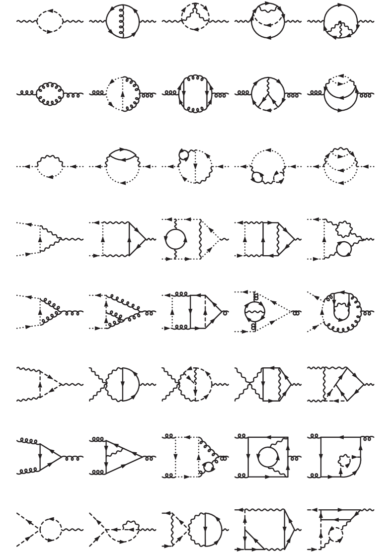
Figure 1: Sample Feynman diagrams contributing to the Green’s functions which have been used for the calculation of the renormalization constants of the gauge couplings. Solid, dashed, dotted, curly and wavy lines correspond to fermions, Higgs bosons, ghosts, gluons and electroweak gauge bosons, respectively.

In the second approach we have used the SM Lagrangian in the background field gauge (BFG) as a starting point (see, e.g., Ref. [22]). The advantage of this method is that only the gauge boson two-point functions and thus less different Green’s functions have to be considered. On the other hand more vertices are present and thus more Feynman diagrams contribute to the background gauge boson propagator as compared to the corresponding quantum version. We use the BFG in the broken phase of the SM. However, here we can also set the masses of all particles to zero. Sample Feynman diagrams for the gauge boson two-point functions are shown in the first and second row of Fig. 1 where the external lines correspond to background gluon, photon and $W$ or $Z$ bosons.

An important issue for all loop calculations involving electroweak gauge bosons is the treatment of $\gamma^{5}$ in $d\not=4$ dimensions. In our calculation we on purpose do not use Green’s functions involving external fermions. For all other two- and three-point functions we could show that a naive treatment of $\gamma^{5}$ leads to the correct result [3]. Note that Green’s functions with external fermions are unavoidable for the calculation of the beta functions for the Yukawa couplings. At two-loop order it is again possible to use a naive version of $\gamma_{5}$. Beyond two loops, however, a more careful treatment is required (see, e.g., Ref. [23]).

We have performed several checks which convinced us from the correctness of our results. In brief they are given by:

• comparison of the one- and two-loop results with the literature

• comparison of partial three-loop results with the literature

• computation of the beta function for the Higgs boson self-coupling to one-loop order and comparison with the literature

• computation of the Yukawa beta functions for the top and bottom quark, and the tau lepton to two-loop order and comparison with the literature

• computation of the $BBB$ vertex to three-loop order; we checked that the sum of all 358 716 diagrams gives zero

• computation for general gauge parameters; we checked that they drop out in the final result for $\beta$ functions

• check that no infra-red divergences are present in the loop integrals

As a last comment on the technical details of our calculation let us mention that we were able to obtain the final result for the gauge coupling beta functions for a general Yukawa structure involving all nine Yukawa couplings of the SM and the CKM matrix in the quark sector. Furthermore, it is straightforward to extend our final result for a SM with fourth family as will be explained in the next section.

3 Results

In this section we briefly discuss the final results for the gauge coupling beta functions. In order to show the structure of the analytical expressions we present the result for $\beta_{1}$ which is given by

$$\beta_{1} =\frac{\alpha_{1}^{2}}{\left(4\pi\right)^{2}}\bigg{\{}\frac{2}{5}+\frac{16n_{G}}{3}\bigg{\}}$$

$$+\frac{\alpha_{1}^{2}}{\left(4\pi\right)^{3}}\bigg{\{}\frac{18\alpha_{1}}{25}+\frac{18\alpha_{2}}{5}-\frac{34\text{tr}\hat{T}}{5}-2\text{tr}\hat{B}-6\text{tr}\hat{L}+n_{G}\bigg{[}\frac{76\alpha_{1}}{15}+\frac{12\alpha_{2}}{5}+\frac{176\alpha_{3}}{15}\bigg{]}\bigg{\}}$$

$$+\frac{\alpha_{1}^{2}}{\left(4\pi\right)^{4}}\bigg{\{}\frac{489\alpha_{1}^{2}}{2000}+\frac{783\alpha_{1}\alpha_{2}}{200}+\frac{3401\alpha_{2}^{2}}{80}+\frac{54\alpha_{1}\hat{\lambda}}{25}+\frac{18\alpha_{2}\hat{\lambda}}{5}-\frac{36\hat{\lambda}^{2}}{5}-\frac{2827\alpha_{1}\text{tr}\hat{T}}{200}$$

$$-\frac{471\alpha_{2}\text{tr}\hat{T}}{8}-\frac{116\alpha_{3}\text{tr}\hat{T}}{5}-\frac{1267\alpha_{1}\text{tr}\hat{B}}{200}-\frac{1311\alpha_{2}\text{tr}\hat{B}}{40}-\frac{68\alpha_{3}\text{tr}\hat{B}}{5}-\frac{2529\alpha_{1}\text{tr}\hat{L}}{200}$$

$$-\frac{1629\alpha_{2}\text{tr}\hat{L}}{40}+\frac{183\text{tr}\hat{B}^{2}}{20}+\frac{51(\text{tr}\hat{B})^{2}}{10}+\frac{157\text{tr}\hat{B}\text{tr}\hat{L}}{5}+\frac{261\text{tr}\hat{L}^{2}}{20}+\frac{99(\text{tr}\hat{L})^{2}}{10}$$

$$+\frac{3\text{tr}\hat{T}\hat{B}}{2}+\frac{339\text{tr}\hat{T}^{2}}{20}+\frac{177\text{tr}\hat{T}\text{tr}\hat{B}}{5}+\frac{199\text{tr}\hat{T}\text{tr}\hat{L}}{5}+\frac{303(\text{tr}\hat{T})^{2}}{10}$$

$$+n_{G}\bigg{[}-\frac{232\alpha_{1}^{2}}{75}-\frac{7\alpha_{1}\alpha_{2}}{25}+\frac{166\alpha_{2}^{2}}{15}-\frac{548\alpha_{1}\alpha_{3}}{225}-\frac{4\alpha_{2}\alpha_{3}}{5}+\frac{1100\alpha_{3}^{2}}{9}\bigg{]}$$

$$+n_{G}^{2}\bigg{[}-\frac{836\alpha_{1}^{2}}{135}-\frac{44\alpha_{2}^{2}}{15}-\frac{1936\alpha_{3}^{2}}{135}\bigg{]}\bigg{\}}\,,$$ (5)

where the limit $\epsilon\to 0$ has been taken. For each gauge coupling beta function we have that the one-loop contribution of $\beta_{i}$ is proportional to $\alpha_{i}^{2}$. Mixed contributions of order $\alpha_{i}^{2}\alpha_{j}$ and $\alpha_{i}^{2}\alpha_{k}\alpha_{l}$ only appear at two and three loops, respectively, where $\alpha_{j}$ are gauge or Yukawa and $\alpha_{k}$ and $\alpha_{l}$ are gauge, Yukawa or Higgs boson self couplings. Note that the latter appears for the first time at three-loop order.

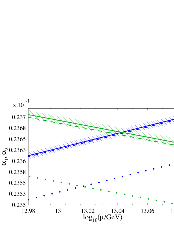
Figure 2: The running of the electroweak gauge couplings in the SM. The lines with positive slope correspond to $\alpha_{1}$, the lines with negative slope to $\alpha_{2}$. The dotted, dashed and solid lines correspond to one-, two- and three-loop precision, respectively. The bands around the three-loop curves visualize the experimental uncertainty.

The symbol $n_{G}$ in Eq. (5) stands for the number of generations; in the SM we have $n_{G}=3$. The quantities $\text{tr}\hat{B}$, $\text{tr}\hat{T}$ and $\text{tr}\hat{L}$ incorporate the Yukawa couplings where we refer to Ref. [3] for details. In this contribution we only want to mention that the replacements

$$\text{tr}\hat{L}^{n}\to\alpha_{\tau}^{n}\,,\quad\text{tr}\hat{T}^{n}\to\alpha_{t}^{n}\,,\quad\text{tr}\hat{B}^{n}\to\alpha_{b}^{n}\,,\quad\text{tr}\hat{T}\hat{B}\to\alpha_{t}\alpha_{b}\,,$$ (6)

leads to the result where only the Yukawa coupling of the third generation is kept non-zero.

In a similar way we can accommodate a fourth generation of fermions. In this case, the Yukawa matrices become $4\times 4$ dimensional. If we assume that the fourth is much heavier and if we neglect all SM Yukawa interactions it contains a $3\times 3$ zero matrix and we have

$$\hat{F_{4}}=\left(\begin{matrix}0_{3\times 3}&0\\ 0&\alpha_{F}\end{matrix}\right)\,,\quad\mbox{with}\quad F=T,B,L\,,$$ (7)

where $T$ and $B$ stand for the up- and down-type heavy quarks, and $L$ for the heavy charged and neutral leptons, while $\alpha_{F}=\frac{\alpha m_{F}^{2}}{2\sin^{2}\theta_{W}M_{W}^{2}}$ denotes the corresponding Yukawa couplings. Note that the contribution of a heavy neutrino is not contained in our formulae.

Let us finally briefly discuss the numerical impact of the new three-loop corrections. In Fig. 2 we show the running of $\alpha_{1}$ and $\alpha_{2}$ from $\mu=M_{Z}$ to the energy scales where these two coupling become equal. The dotted and dashed lines correspond to one- and two-loop running, respectively. One observes a significant change of the curves, which is in particular much bigger than the experimental uncertainty indicated by the dashed band. Thus in case only one- and two-loop perturbative corrections are included the theory uncertainty is much bigger than the experimental one. This changes with the inclusion of the three-loop terms. The results are shown as solid lines which are close to the corresponding dashed curves. The effect is small, however, still of the order of the experimental uncertainty, in particular for $\alpha_{2}$.

To conclude, the complete three-loop corrections to the gauge coupling beta functions have been computed [2, 3] using different methods and applying several cross checks. They constitute fundamental quantities of the SM and are important for high-precision experimental checks.

References

- [1] K. G. Chetyrkin and F. V. Tkachov, Nucl. Phys. B 192 (1981) 159.
- [2] L. N. Mihaila, J. Salomon and M. Steinhauser, Phys. Rev. Lett. 108 (2012) 151602 [arXiv:1201.5868 [hep-ph]].
- [3] L. N. Mihaila, J. Salomon and M. Steinhauser, [arXiv:1208.3357 [hep-ph]].
- [4] D. J. Gross and F. Wilczek, Phys. Rev. Lett. 30 (1973) 1343.
- [5] H. D. Politzer, Phys. Rev. Lett. 30 (1973) 1346.
- [6] D. R. T. Jones, Nucl. Phys. B 75, 531 (1974).
- [7] O. V. Tarasov and A. A. Vladimirov, Sov. J. Nucl. Phys. 25 (1977) 585 [Yad. Fiz. 25 (1977) 1104].
- [8] W. E. Caswell, Phys. Rev. Lett. 33 (1974) 244.
- [9] E. Egorian and O. V. Tarasov, Teor. Mat. Fiz. 41 (1979) 26 [Theor. Math. Phys. 41 (1979) 863].
- [10] D. R. T. Jones, Phys. Rev. D 25 (1982) 581.
- [11] M. S. Fischler and C. T. Hill, Nucl. Phys. B 193 (1981) 53.
- [12] M. E. Machacek and M. T. Vaughn, Nucl. Phys. B 222 (1983) 83.
- [13] I. Jack and H. Osborn, Nucl. Phys. B 249 (1985) 472.
- [14] T. Curtright, Phys. Rev. D 21 (1980) 1543.
- [15] D. R. T. Jones, Phys. Rev. D 22 (1980) 3140.
- [16] O. V. Tarasov, A. A. Vladimirov and A. Y. Zharkov, Phys. Lett. B 93 (1980) 429.
- [17] S. A. Larin and J. A. M. Vermaseren, Phys. Lett. B 303 (1993) 334 [hep-ph/9302208].
- [18] M. Steinhauser, Phys. Rev. D 59 (1999) 054005 [arXiv:hep-ph/9809507].
- [19] A. G. M. Pickering, J. A. Gracey and D. R. T. Jones, Phys. Lett. B 510 (2001) 347 [Phys. Lett. B 512 (2001 ERRAT,B535,377.2002) 230] [arXiv:hep-ph/0104247].
- [20] T. van Ritbergen, J. A. M. Vermaseren and S. A. Larin, Phys. Lett. B 400 (1997) 379 [hep-ph/9701390].
- [21] M. Czakon, Nucl. Phys. B 710 (2005) 485 [arXiv:hep-ph/0411261].
- [22] A. Denner, G. Weiglein and S. Dittmaier, Nucl. Phys. B 440 (1995) 95 [hep-ph/9410338].
- [23] K. G. Chetyrkin and M. F. Zoller, JHEP 1206 (2012) 033 [arXiv:1205.2892 [hep-ph]].