Dynamics of Dirac-Born-Infeld dark energy interacting with dark matter

Abstract

We study the dynamics of Dirac-Born-Infeld (DBI) dark energy interacting with dark matter. The DBI dark energy model considered here has a scalar field with a nonstandard kinetic energy term, and has potential and brane tension that are power-law functions. The new feature considered here is an interaction between the DBI dark energy and dark matter through a phenomenological interaction between the DBI scalar field and the dark matter fluid. We analyze two different types of interactions between the DBI scalar field and the dark matter fluid. In particular we study the phase-space diagrams of and look for critical points of the phase space that are both stable and lead to accelerated, late-time expansion. In general we find that the interaction between the two dark components does not appear to give rise to late-time accelerated expansion. However, the interaction can make the critical points in the phase space of the system stable. Whether such stabilization occurs or not depends on the form of the interaction between the two dark components.

I Introduction

In recent years much of the effort in theoretical physics has gone into the study of the observed present accelerated expansion of the Universe first reported in Perlmutter_1999 ; Riess_1998 through observational data from Type Ia supernovae. Subsequent work on Type Ia supernovae Hicken , the cosmic microwave background Komatsu;2009 , and baryon acoustic oscillations Percival;2007 , all support the initial observations that the expansion of the Universe is accelerating. This late-time acceleration of the Universe is driven by a fluid/field generically called dark energy. Very little is known about dark energy. Within the context of string theory there is a model for the early-time accelerated expansion of the Universe associated with inflation. This string-theory-motivated model for inflation is called Dirac-Born-Infield (DBI) inflation Silverstein_Tong;2004 ; Alishahiha_Silverstein_Tong;2004 ; Chen_prd;2005 ; Chen_jhep;2005 ; Shandera_Tye;2006 ; Gumjudpai;2004 , and it is driven by the open string sector through dynamical Dp-branes. DBI inflation is a special case of K-inflation models Armendariz;1999 . It was originally thought that DBI inflation models would yield large non-Gaussian perturbations which could be used to verify or falsify these models and by extension to test string theory Gumjudpai;2004 ; Chimento;2009 . However, subsequent work has shown that this may not be the case, and that the simplest DBI models are effectively indistinguishable from standard field-theoretic slow-roll models of inflation Lidsey;2007 .

In the present work we examine variants of these DBI models as a mechanism, not for the early-time acceleration of inflation, but for the observed late-time acceleration. Our DBI scalar field will play the role of dark energy. The action for our scalar DBI field is taken to have the form found in Ref. Chimento;2009 .

$$S_{DBI}=-\int\mathrm{d}^{4}x\sqrt{-g}\left[T(\phi)\sqrt{1-\frac{\dot{\phi}^{2}}{T}}+V(\phi)-T(\phi)\right]~{},$$ (1)

where we have assumed that the scalar DBI field , $\phi$, is spatially homogeneous so that its spatial derivatives can be ignored. This is in accord with the fact that dark energy seems to be very homogeneously distributed. Note that $\phi$ has a nonstandard kinetic energy term which yields a standard kinetic energy term if one expands the square root to first order in $\frac{\dot{\phi}^{2}}{T}$. For a pure AdS₅ geometry with radius $R$, the warped tension $T(\phi)=\tau\phi^{4}$ is the D3-brane tension with $\tau=1/(g_{s}\tilde{\lambda})$, where $g_{s}$ is the string coupling, $\alpha^{\prime}$ is the inverse string tension, and $\tilde{\lambda}=R^{4}/\alpha^{\prime}$ is the ’t Hooft coupling in the AdS/CFT correspondence. $V(\phi)$ is the potential arising from interactions with Ramond-Ramond fluxes or with other sectors Silverstein_Tong;2004 . Here we take the potential to be quadratic, $V(\phi)=m^{2}\phi^{2}$, and the associated D-brane is in the anti-de Sitter throat Guo_ Ohta;2008 .

In a spatially flat Friedmann-Robertson-Walker (FRW) metric with scale factor $a(t)$, it can be shown that the energy density $\rho_{\phi}$ and the pressure $p_{\phi}$ of the DBI scalar field are given by

$$\rho_{\phi}=\frac{\gamma^{2}}{\gamma+1}\,\dot{\phi}^{2}+V(\phi)\quad\mathrm{and}\quad p_{\phi}=\frac{\gamma}{\gamma+1}\,\dot{\phi}^{2}-V(\phi),$$ (2)

where $\gamma$ has the form of a Lorentz boost factor,

$$\gamma\equiv\frac{1}{\sqrt{1-\frac{\dot{\phi}^{2}}{T(\phi)}}}.$$ (3)

In this paper we analyze this system of a DBI dark energy field interacting with dark matter in terms of late-time scaling solutions. Such models are different from the original work in Ref. Copeland_Mizuno_Shaeri;2010 which studied the dynamics of a DBI field plus a perfect fluid but with no interaction between the DBI field and the perfect fluid. In the course of our analysis of this model of DBI dark energy interacting with dark matter, we find that for certain parameters there are late-time attractor solutions or fixed points in the phase space of the parameters.

The organization of the rest of the paper is as follows. In Sec. II, we write down two possible phenomenological interactions between the DBI dark energy scalar field with the dark matter fluid. In Sec. III, we analyze the autonomous equations in terms of the relevant variables of DBI dark energy interacting with dark matter. We find the fixed points in the phase-space flow of these variables. We also discuss the stability (i.e. stable fixed point, unstable fixed point or saddle fixed point) of fixed points and determine if the fixed points correspond to late-time accelerated expansion or not. Of particular importance will be stable fixed points which lead to late-time accelerated expansion. Finally, we summarize our results in Sec. IV.

II DBI dark energy scalar field interacting with dark matter

Cosmological evolution is thought to be largely dominated by dark energy and dark matter. Dark energy gives a gravitationally repulsive effect while dark matter is gravitationally attractive. Usually there is no interaction between these two components such as in the model in Ref.chaves-2007 where graded Lie algebras were used to give a unified theory with both dark energy and dark matter, but without any interaction between these two components.

There has been work such as the two measure cosmological model of Ref. guendelman where there is some interaction between the dark energy and dark matter components of the model. However, since the gravitational effects of dark energy and dark matter are opposite (i.e., gravitational repulsion versus gravitational attraction) and since dark energy appears to be very homogeneously distributed, while dark matter clumps around ordinary matter, one expects that any interaction between these two dark components of the Universe would be weak. In this paper we will consider models where there is an interaction between dark energy and dark matter. The dark energy component will come from the DBI scalar field in Eq. (1) with energy density $\rho_{\phi}$ and pressure $p_{\phi}$, and the dark matter component will come from a fluid with an equation of state $w_{m}\equiv p_{m}/\rho_{m}=0$. Considering a spatially flat Friedman-Robertson-Walker background with scale factor $a(t)$, and allowing for creation/annihilation between the DBI scalar field and the dark matter fluid at a rate $Q$, we can write down the equations for $\rho_{\phi}$ and $\rho_{m}$ as

$$\dot{\rho}_{\phi}+3H\left(1+w_{\phi}\right)\rho_{\phi} = -Q$$ (4)

$$\dot{\rho}_{m}+3H\rho_{m} = +Q~{}.$$ (5)

Here $H\equiv\dot{a}/a$ is the Hubble rate with derivatives with respect to cosmological time, $t$, being indicated by a dot. The DBI scalar field and the dark matter create/decay into one another via the common creation/annihilation rate $\pm Q$. $Q$ represents the interaction between these two fields. Although at this point this interaction is generic, one can say that if $Q>0$ dark energy converts to dark matter, and if $Q<0$ dark matter is converted to dark energy couplingmodels .

Since there is no fundamental theory which specifies a coupling between dark energy and dark matter, our coupling models will necessarily be phenomenological, although one might view some couplings as more physical or more natural than others. In this paper we consider two types of coupling:

$$\mathrm{Model~{}I}\quad Q =\sqrt{\frac{2}{3}}\beta\rho_{m}\dot{\phi},$$ (6)

$$\mathrm{Model~{}II}\quad Q =\alpha H\rho_{m}$$ (7)

where $\beta$ and $\alpha$ are dimensionless constants whose sign determines the direction of energy transfer. For positive values of the parameters $\alpha,\beta>0$ ($Q>0$) there is a transfer of energy from DBI dark energy to dark matter; for negative values of the parameters $\alpha,\beta<0$ ($Q<0$) there is a transfer of energy from dark matter to DBI dark energy.

The interaction given in Model I may be motivated within the context of scalar-tensor theories Wetterich;1995 ; Amendola;1999 ; Holden_Wards;2000 where similar interaction terms can be found. Generalizations of this model allow for $\beta=\beta(\phi)$ and more general forms of $V(\phi)$ (e.g., Refs. Huey_Wandelt;2006 ; Bean_Magueijo;2001 ). Interactions of the form given by Model II have been considered in Ref. Zimdahl_ Pavon;2001 which used $Q/H=\alpha_{m}\rho_{m}+\alpha_{\phi}\rho_{\phi}$ and in Ref. Guo_ Ohta;2007 , which used $Q/H=\alpha\Omega_{\phi}$.

The equation for the rate of change of the Hubble parameter is

$$\dot{H}=-\frac{1}{2}\left[\left(1+w_{\phi}\right)\rho_{\phi}+\rho_{m}\right]$$ (8)

The Hubble parameter is subject to the constraint

$$H^{2}=\frac{1}{3}(\rho_{\phi}+\rho_{m})~{}.$$ (9)

In this work we use the units such that $8\pi G=1$, where $G$ is Newton’s gravitational constant.

We define the fractional density of the DBI dark energy and dark matter via $\Omega_{\phi}\equiv\rho_{\phi}/3H^{2}$ and $\Omega_{m}\equiv\rho_{m}/3H^{2}$, with the condition that $\Omega_{\phi}+\Omega_{m}=1$ which comes from (9). The modified Klein-Gordon equation, which follows from Eqs.(2), (4), and (8) and gives the evolution of the DBI scalar field, takes the form

$$\ddot{\phi}+\frac{3H}{\gamma^{2}}\dot{\phi}+\frac{V_{,\phi}}{\gamma^{3}}-\frac{T_{,\phi}}{2T}\frac{(\gamma+2)(\gamma-1)}{(\gamma+1)\gamma}\,\dot{\phi}^{2}=-\frac{Q}{\gamma^{3}\dot{\phi}}~{},$$ (10)

where $V_{,\phi}\equiv\mathrm{d}V(\phi)/\mathrm{d}\phi$ and $T_{,\phi}\equiv\mathrm{d}T(\phi)/\mathrm{d}\phi$. Eqs. (5), (8), and (10) give a closed system of equations that determines the dynamics of the DBI dark energy scalar field, $\phi$, interacting with dark matter.

In order to find the fixed points of this system and to study the late-time attractor behavior of these two models we introduce the following set of dimensionless variables similar to those used in Ref. Copeland_Liddle;1998 :

$$x\equiv\frac{\gamma\dot{\phi}}{\sqrt{3(\gamma+1)}H},\quad y\equiv\frac{\sqrt{V}}{\sqrt{3}H}.$$ (11)

With $x$ and $y$ defined in this way we can recover the variables for the scalar field model originally proposed in Ref. Copeland_Liddle;1998 by taking the limit $\gamma\to 1$. The variable $x$ roughly corresponds to the the kinetic energy of the DBI field, while $y$ roughly corresponds to the potential energy of the DBI field. In addition to these dynamical variables $x$ and $y$ we introduce a third variable $\tilde{\gamma}=1/\gamma$ which is connected with the brane tension $T(\phi)$. Taking the inverse of $\gamma$ makes the final equations more compact. Thus we have exchanged the three variables $\phi$, $V(\phi)$, and $T(\phi)$ for $x$, $y$, and $\tilde{\gamma}$.

In terms of these variables, the Friedmann constraint from Eq. (8) can be expressed as

$$x^{2}+y^{2}+\Omega_{m}=\Omega_{\phi}+\Omega_{m}=1.$$ (12)

The equation of state of the DBI dark energy is given by

$$w_{\phi}=\frac{\rho_{\phi}}{p_{\phi}}=\frac{\tilde{\gamma}x^{2}-y^{2}}{x^{2}+y^{2}}.$$ (13)

Finally, we introduce two sets of variables related to the potential, $V(\phi)$, and the brane tension, $T(\phi)$. The first set, $\lambda_{1}$ and $\lambda_{2}$, are defined as

$$\lambda_{1}\equiv-\frac{V_{,\phi}}{V},\qquad\lambda_{2}\equiv-\frac{T_{,\phi}}{T}~{}.$$ (14)

The second set of variables, $\tilde{\lambda}_{1}$ and $\tilde{\lambda}_{2}$, are given by

$$\tilde{\lambda}_{1}\equiv-\frac{V_{,\phi}}{T^{-1/2}V^{3/2}},\qquad\tilde{\lambda}_{2}\equiv-\frac{T_{,\phi}}{T^{1/2}V^{1/2}}$$ (15)

The relationship between the two sets of variables (14) and (15) is given by

$$\lambda_{1}=\sqrt{\frac{(1-\tilde{\gamma})}{\tilde{\gamma}}}\frac{y}{x}\tilde{\lambda}_{1},\qquad\lambda_{2}=\sqrt{\frac{(1-\tilde{\gamma})}{\tilde{\gamma}}}\frac{y}{x}\tilde{\lambda}_{2}.$$ (16)

Combining the above definitions, the evolution equations for $x$, $y$ and ${\tilde{\gamma}}$ can be written as the following autonomous system:

$$\frac{\mathrm{d}x}{\mathrm{d}N}= \frac{\tilde{\lambda}_{1}y^{3}\sqrt{3(1-\tilde{\gamma}^{2})}}{2x}-\frac{Q}{6xH^{3}}+\frac{3x}{2}\left\{\tilde{\gamma}(x^{2}-1)-y^{2}\right\}$$

$$\frac{\mathrm{d}y}{\mathrm{d}N}= -\frac{\tilde{\lambda}_{1}y^{2}\sqrt{3(1-\tilde{\gamma}^{2})}}{2}+\frac{3y}{2}\left\{1+\tilde{\gamma}x^{2}-y^{2}\right\}$$ (18)

$$\frac{\mathrm{d}\tilde{\gamma}}{\mathrm{d}N}= \frac{\tilde{\gamma}(1-\tilde{\gamma}^{2})}{\sqrt{(1+\tilde{\gamma})}}\!\!\left[3\sqrt{(1+\tilde{\gamma})}\!\!-\!\!\sqrt{3(1-\tilde{\gamma})}\frac{y}{x^{2}}\!\left[\tilde{\lambda}_{1}y^{2}+\tilde{\lambda}_{2}x^{2}\right]\right.$$ (19)

$$\qquad\qquad\quad\quad\left.+\frac{Q}{x^{2}\sqrt{3(1+\tilde{\gamma})}H^{3}}\!\right]$$

where $N\equiv\ln{a}$ and $\frac{\mathrm{d}\,\,}{\mathrm{d}N}=\frac{1}{H}\frac{\mathrm{d}\,\,}{\mathrm{d}t}$. There are also two equations for $\lambda_{1}$ and $\lambda_{2}$

$$\frac{\mathrm{d}\lambda_{1}}{\mathrm{d}N}= -x\lambda_{1}^{2}\sqrt{3\tilde{\gamma}(1+\tilde{\gamma})}\left\{\frac{VV_{,\,\phi\phi}}{V^{2}_{,\,\phi}}-1\right\},$$ (20)

$$\frac{\mathrm{d}\lambda_{2}}{\mathrm{d}N}= -x\lambda_{2}^{2}\sqrt{3\tilde{\gamma}(1+\tilde{\gamma})}\left\{\frac{TT_{,\,\phi\phi}}{T^{2}_{,\,\phi}}-1\right\}\;.$$ (21)

Since $\mathrm{d}\lambda_{1}/\mathrm{d}N$ and $\mathrm{d}\lambda_{2}/\mathrm{d}N$ can be expressed in terms of $\mathrm{d}x/\mathrm{d}N$, $\mathrm{d}y/\mathrm{d}N$, $\mathrm{d}\tilde{\gamma}/\mathrm{d}N$ from Eqs. (LABEL:eq17) - (19), thus equations Eqs. (20) and (21) are not independent equations and we only need to solve three equations for $x$, $y$, and ${\tilde{\gamma}}$. The time evolution equation for $H$ given in Eq. (8) can be rewritten by differentiating the Hubble parameter with respect to $N$, which yields

$$\frac{1}{H}\frac{\mathrm{d}H}{\mathrm{d}N}=-\frac{3}{2}\left\{1+\tilde{\gamma}x^{2}-y^{2}\right\}.$$ (22)

The total effective equation of state for the DBI scalar field plus dark matter can be written as

$$w_{\mathrm{eff}}=\frac{p_{\phi}+p_{m}}{\rho_{\phi}+\rho_{m}}=\tilde{\gamma}x^{2}-y^{2}.$$ (23)

In the next section we will investigate the two different models, given by Eqs. (6) and (7), near critical points ($x_{c}$, $y_{c}$). Near a critical point the scale factor of the FRW space-time takes the form

$$a\propto t^{2/3(1+\tilde{\gamma}x^{2}_{c}-y^{2}_{c})}\;.$$ (24)

In order to have accelerated expansion (i.e. $\ddot{a}>0$) the above equation requires that $w_{\mathrm{eff}}=\tilde{\gamma}x^{2}_{c}-y^{2}_{c}<-\frac{1}{3}$. Combining Eq. (22) with Eq. (23), and recalling that $\frac{\mathrm{d}\,\,}{\mathrm{d}N}=\frac{1}{H}\frac{\mathrm{d}\,\,}{\mathrm{d}t}$, the Hubble parameter evolution equation becomes

$$\frac{\dot{H}}{H^{2}}=-\frac{3(1+w_{\mathrm{eff}})}{2}.$$ (25)

The energy balance equations (4) and (5) for Model I and Model II are independent of $H$ when expressed in terms of the variables $x(N)$ and $y(N)$, where $N=\ln a$. Thus the Hubble parameter evolution equation (25) is not needed for these particular interacting models, and the phase space of both models is a two-dimensional phase space involving $x$ and $y$.

III Critical points and stability analysis

In this section we find the critical or fixed points of the autonomous system Eqs. (LABEL:eq17) - (19) and perform a stability analysis of these fixed points. We are looking for the late-time attractor structure of this system of a DBI scalar field interacting with dark matter via an energy exchange given by $Q$. The fixed points for Eqs. (LABEL:eq17) - (19) are found by setting $dx/dN=dy/dN=d{\tilde{\gamma}}/dN=0$ and solving the resulting three algebraic equations for the critical $x_{c},y_{c},$ and ${\tilde{\gamma}}_{c}$. Additionally, we will focus on the case when ${\tilde{\gamma}}_{c}=0$ [from Eq. (3) this implies $\gamma=\infty$] or ${\tilde{\gamma}}_{c}=1$ [from Eq. (3) this implies $\gamma=1$]. Thus ${\tilde{\gamma}}$ is constant and the autonomous system reduces to only two dynamical variables: $x$ and $y$.

After finding the fixed points we study their stability with respect to small perturbations, $\delta x$ and $\delta y$, about the critical points $x_{c}$, $y_{c}$. Explicitly, these take the form

$$x=x_{c}+\delta x,\quad y=y_{c}+\delta y\;.$$ (26)

Substituting Eq. (26) into Eqs. (LABEL:eq17) and (18), and keeping terms up to first order in $\delta x$ and $\delta y$, leads to a system of first-order differential equations of the form

$$\frac{\mathrm{d}}{\mathrm{d}N}\left({\begin{array}[]{*{20}{c}}{\delta x}\\ {\delta y}\\ \end{array}}\right)=\mathcal{M}\left({\begin{array}[]{*{20}{c}}{\delta x}\\ {\delta y}\\ \end{array}}\right)\>,$$ (27)

where $\mathcal{M}$ is a $2\times 2$ matrix that depends on $x_{c}$ and $y_{c}$. To study the stability around the fixed points one calculates the eigenvalues of $\mathcal{M}$. We denote these eigenvalues as $\mu_{1}$ and $\mu_{2}$, and for every critical point $(x_{c},y_{c})$ there is an associated eigenvalue pair $(\mu_{1},\mu_{2})$. The stability of the critical point $(x_{c},y_{c})$ is then determined by its associated eigenvalue pair $(\mu_{1},\mu_{2})$ in the following way: (i) if $\mu_{1}<0$ and $\mu_{2}<0$, then the critical point is stable; (ii) if $\mu_{1}>0$ and $\mu_{2}>0$, then the critical point is unstable; (iii) if $\mu_{1}<0$ and $\mu_{2}>0$ or $\mu_{1}>0$ and $\mu_{2}<0$, then one has a saddle point; (iv) if the determinant of the matrix $\mathcal{M}$ is negative and the real parts of $\mu_{1}$ and $\mu_{2}$ are negative, then one has a limit cycle. For our two models, Model I and Model II, all the fixed points fall into cases (i), (ii), or (iii). None of the fixed point we found are limit cycles.

III.1 Interacting Model I $Q=\sqrt{\frac{2}{3}}\beta\rho_{m}\dot{\phi}$

Recalling that we are taking ${\tilde{\gamma}}$ to be a nondynamical constant with a value of $0$ or $1$ our autonomous system (LABEL:eq17) - (18) for Model I (6) becomes

$$\frac{\mathrm{d}x}{\mathrm{d}N}=\frac{\tilde{\lambda}_{1}y^{3}\sqrt{3(1-\tilde{\gamma}^{2})}}{2x}-\frac{\beta\sqrt{2\tilde{\gamma}(1+\tilde{\gamma})}[1-x^{2}-y^{2}]}{2}$$

$$\qquad+\frac{3x}{2}\left\{\tilde{\gamma}\left(x^{2}-1\right)-y^{2}\right\}$$ (28)

$$\frac{\mathrm{d}y}{\mathrm{d}N}=-\frac{\tilde{\lambda}_{1}y^{2}\sqrt{3(1-\tilde{\gamma}^{2})}}{2}+\frac{3y}{2}\left\{1+\tilde{\gamma}x^{2}-y^{2}\right\}$$ (29)

The dynamics of this autonomous system is determined by the parameters $\beta$ and $\tilde{\lambda}_{1}$.

The fixed points for Eqs. (28) and (29) are obtained by setting $dx/dN=0$ and $dy/dN=0$ and solving the resulting algebraic equations for $x_{c}$ and $y_{c}$. There are six fixed points and these are presented in the first two columns of Table 1.

Table 1: The fixed points for Model I with $Q=\sqrt{\frac{2}{3}}\beta\rho_{m}\dot{\phi}$.

Fixed point	$x_{c}$	$y_{c}$	$\tilde{\gamma}$	$\Omega_{\phi}$	$w_{\phi}$	$w_{\mathrm{eff}}$
(a1)	$-\sqrt{\frac{\tilde{\lambda}_{1}\left(\sqrt{\tilde{\lambda}^{2}_{1}+12}-\tilde{\lambda}_{1}\right)}{6}}$	$\frac{\sqrt{\tilde{\lambda}^{2}_{1}+12}-\tilde{\lambda}_{1}}{2\sqrt{3}}$	$0$	$1$	$-\frac{[\sqrt{\tilde{\lambda}^{2}_{1}+12}-\tilde{\lambda}_{1}]^{2}}{12}$	$-\frac{[\sqrt{\tilde{\lambda}^{2}_{1}+12}-\tilde{\lambda}_{1}]^{2}}{12}$
(a2)	$\sqrt{\frac{\tilde{\lambda}_{1}\left(\sqrt{\tilde{\lambda}^{2}_{1}+12}-\tilde{\lambda}_{1}\right)}{6}}$	$\frac{\sqrt{\tilde{\lambda}^{2}_{1}+12}-\tilde{\lambda}_{1}}{2\sqrt{3}}$	$0$	$1$	$-\frac{[\sqrt{\tilde{\lambda}^{2}_{1}+12}-\tilde{\lambda}_{1}]^{2}}{12}$	$-\frac{[\sqrt{\tilde{\lambda}^{2}_{1}+12}-\tilde{\lambda}_{1}]^{2}}{12}$
(b1)	$-1$	$0$	$1$	$1$	$1$	$1$
(b2)	$0$	$1$	$1$	$1$	$-1$	$-1$
(b3)	$1$	0	$1$	$1$	$1$	$1$
(b4)	$-\frac{2\beta}{3}$	0	$1$	$\frac{4\beta^{2}}{9}$	$1$	$\frac{4\beta^{2}}{9}$

We call the fixed points (a1)-(a2) “ultrarelativistic” fixed points since for them the Lorentz factor $\gamma$ [Eq. (3)] tends to infinity (which implies that $\tilde{\gamma}=0$). There are also an infinite number of “trivial” fixed points for which ${\tilde{\gamma}}_{c}=y_{c}=0$ and for which $x_{c}$ is arbitrary within the range constrained by $0<x_{c}<\sqrt{1-\Omega_{m}}$ ($\Omega_{m}$ is the previously defined fractional density of dark matter). These unstable, “trivial” critical points are shown along the $y=0$ axis in Fig. 1. The four other critical points (b1)-(b4) listed in Table 1 are “standard” fixed points since for these fixed points the Lorentz factor of Eq. (3) equals $1$ (so that $\tilde{\gamma}=1$), and the DBI field will mimic the behavior of a canonical scalar field.

III.1.1 Stability of the fixed points in Model I

For each of the six fixed points listed in Table 1 we found the eigenvalues $\mu_{1}$ and $\mu_{2}$ of the matrix $\mathcal{M}$ in Eq. (27). The results for each point are listed below along with whether the point is stable, unstable, or a saddle point

• Point (a1):
  $\mu_{1}=-\frac{1}{4}\left(\tilde{\lambda}_{1}-\sqrt{\tilde{\lambda}^{2}_{1}+12}\right)^{2}$ ,
  $\mu_{2}=\frac{1}{4}\left(-\tilde{\lambda}^{2}_{1}+\tilde{\lambda}_{1}\sqrt{\tilde{\lambda}^{2}_{1}+12}-12\right)$.
  This point is stable for all values of $\tilde{\lambda}_{1}$.

• Point (a2):
  $\mu_{1}=-\frac{1}{4}\left(\tilde{\lambda}_{1}-\sqrt{\tilde{\lambda}^{2}_{1}+12}\right)^{2}$,
  $\mu_{2}=\frac{1}{4}\left(-\tilde{\lambda}^{2}_{1}+\tilde{\lambda}_{1}\sqrt{\tilde{\lambda}^{2}_{1}+12}-12\right)$.
  This point is stable for all values of $\tilde{\lambda}_{1}$.

• Point (b1):
  $\mu_{1}=3$, $\mu_{2}=3-2\beta$.
  This point is a saddle point for $\beta>\frac{3}{2}$ and is unstable for $\beta<\frac{3}{2}$.

• Point (b2):
  $\mu_{1}=-3$, $\mu_{2}=-3$.
  This point is stable for all values of $\beta$ and $\tilde{\lambda}_{1}$.

• Point (b3):
  $\mu_{1}=3$, $\mu_{2}=2\beta+3$.
  This point is unstable for $\beta>-\frac{3}{2}$ and is a saddle point for $\beta>-\frac{3}{2}$.

• Point (b4):
  $\mu_{1}=\frac{1}{6}\left(4\beta^{2}-9\right)$, $\mu_{2}=\frac{1}{6}\left(4\beta^{2}+9\right)$.
  This point is unstable for $\beta>\frac{3}{2}$ or $\beta<-\frac{3}{2}$ and is a saddle point for -$\frac{3}{2}<\beta<\frac{3}{2}$.

Table 2: The conditions for stability, acceleration and existence of the fixed point for Model I in terms of the parameters $\beta$ and $\tilde{\lambda}_{1}$.

Fixed point	Stability	Acceleration	Existence
(a1)	Stable node for all values of $\tilde{\lambda}_{1}$	$\tilde{\lambda}_{1}<2$	all $\beta$, $\tilde{\lambda}_{1}$
(a2)	Stable node for all values of $\tilde{\lambda}_{1}$	$\tilde{\lambda}_{1}<2$	all $\beta$, $\tilde{\lambda}_{1}$
(b1)	Saddle point for $\beta>\frac{3}{2}$	No	$\beta>0$
	Unstable node for $\beta<\frac{3}{2}$
(b2)	Stable node for all values of $\beta$, $\tilde{\lambda}_{1}$	Yes	all $\beta$, $\tilde{\lambda}_{1}$
(b3)	Saddle point for $\beta<-\frac{3}{2}$	No	all $\beta$, $\tilde{\lambda}_{1}$
	Unstable node for $\beta>-\frac{3}{2}$
(b4)	Saddle point for $-\frac{3}{2}<\beta<\frac{3}{2}$	No	$\beta<0$
	Unstable node for $\beta<-\frac{3}{2}$ or $\beta>\frac{3}{2}$

III.1.2 Late-time behavior for model I

In this subsection we investigate the late-time behavior of the scale factor $a(t)$. We are interested in whether $a(t)$ is accelerating, which means that the total effective equation of state parameter for this model should satisfy $w_{\mathrm{eff}}<-\frac{1}{3}$. The six critical points from Table 1 are listed in Table 2 with the conditions under which they are stable, unstable, or saddle points (the second column), the conditions (if any) under which the critical point leads to accelerated expansion (the third column), and the conditions on $\beta,{\tilde{\lambda}}_{1}$ for the critical point to exist (the fourth column).

Table 2 shows that for Model I the two critical points (a1) and (a2) are stable for all values of $\tilde{\lambda}_{1}$ since $\mu_{1},\mu_{2}<0$. Further, these two points lead to accelerated expansion (i.e., $w_{\mathrm{eff}}<-\frac{1}{3}$) if $\tilde{\lambda}_{1}<2$. For these reasons these two attractors are of interest in explaining the observed late-time accelerated expansion of the Universe. The phase-space flow for these two points is shown in Fig. 1.

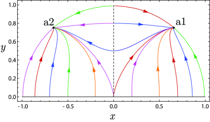
Figure 1: Model I: The $x-y$ phase plane for the DBI dark energy interacting with dark matter. We have taken the parameters as $\beta=1$, $\tilde{\lambda}_{1}=1$, and $\tilde{\gamma}=0$. There are two stable, critical points: a(1) and a(2). Both points lead to accelerated expansion. The dotted line is $x=0$, which is the singularity value of the nonallowed region.

The point (b2) is a stable critical point (i.e., $\mu_{1},\mu_{2}<0$) for all values of $\beta$ and $\tilde{\lambda}_{1}$. Additionally the point (b2) gives accelerated expansion for the Universe (i.e., $w_{\mathrm{eff}}<-\frac{1}{3}$) for all values of $\tilde{\lambda}_{1}$ and $\beta$. The $x-y$ phase-space behavior of the critical point (b2) is shown in Figs. 2 and 3. The remaining critical points -(b1), (b3), and (b4) - are of less interest phenomenologically since they do not lead to accelerated expansion. Thus, there are three fixed points - (a1), (a2), and (b2) - which are stable and lead to late-time accelerated expansion. However, in regard to the existence of these fixed points or their stability the specific value of $\beta$ (the parameter which characterizes the coupling between dark energy and dark matter) plays no role. All these fixed points would exist and be stable even if $\beta=0$, i.e., even in the absence of coupling between dark energy and dark matter. Thus for Model I the overall conclusion is that this coupling does not play a significant role in the late-time behavior of the system.

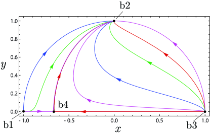
Figure 2: Model I: The $x-y$ phase plane for DBI dark energy interacting with dark matter with the parameters $\beta=1$, $\tilde{\lambda}_{1}=1$ and $\tilde{\gamma}=1$. The point $(b2)$ is a stable critical point which leads to late-time accelerated expansion.

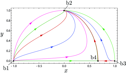
Figure 3: Model I: The $x-y$ phase plane for DBI dark energy interacting with dark matter with the parameters $\beta=-1$, $\tilde{\lambda}_{1}=1$ and $\tilde{\gamma}=1$. The point $(b2)$ is a stable critical point which leads to late-time accelerated expansion.

III.2 Interacting Model II: $Q=\alpha H\rho_{m}$

The autonomous system for the variables $x$ and $y$ is now

$$\frac{\mathrm{d}x}{\mathrm{d}N}=\frac{\tilde{\lambda}_{1}y^{3}\sqrt{3(1-\tilde{\gamma}^{2})}}{2x}-\frac{\alpha}{2x}[1-x^{2}-y^{2}]$$

$$\qquad+\frac{3x}{2}\left\{\tilde{\gamma}\left(x^{2}-1\right)-y^{2}\right\}$$ (30)

$$\frac{\mathrm{d}y}{\mathrm{d}N}=-\frac{\tilde{\lambda}_{1}y^{2}\sqrt{3(1-\tilde{\gamma}^{2})}}{2}+\frac{3y}{2}\left\{1+\tilde{\gamma}x^{2}-y^{2}\right\}$$ (31)

The fixed points are again obtained by setting $dx/dN=0$ and $dy/dN=0$ in Eqs. (30) and (31). For Model II there are eight fixed points - (d1) to (d4) and (e1) to (e4) - and these are listed in Table 3.

Table 3: The fixed points for Model II

Fixed point	$x_{c}$	$y_{c}$	$\tilde{\gamma}$	$\Omega_{\phi}$	$w_{\phi}$	$w_{\mathrm{eff}}$
(d1)	$-1$	0	$0$	$1$	$0$	$0$
(d2)	$1$	0	$0$	$1$	$0$	$0$
(d3)	$-\sqrt{\frac{\tilde{\lambda}_{1}\left(\sqrt{\tilde{\lambda}^{2}_{1}+12}-\tilde{\lambda}_{1}\right)}{6}}$	$\frac{\sqrt{\tilde{\lambda}^{2}_{1}+12}-\tilde{\lambda}_{1}}{2\sqrt{3}}$	$0$	$1$	$-\frac{[\sqrt{\tilde{\lambda}^{2}_{1}+12}-\tilde{\lambda}_{1}]^{2}}{12}$	$-\frac{[\sqrt{\tilde{\lambda}^{2}_{1}+12}-\tilde{\lambda}_{1}]^{2}}{12}$
(d4)	$\sqrt{\frac{\tilde{\lambda}_{1}\left(\sqrt{\tilde{\lambda}^{2}_{1}+12}-\tilde{\lambda}_{1}\right)}{6}}$	$\frac{\sqrt{\tilde{\lambda}^{2}_{1}+12}-\tilde{\lambda}_{1}}{2\sqrt{3}}$	$0$	$1$	$-\frac{[\sqrt{\tilde{\lambda}^{2}_{1}+12}-\tilde{\lambda}_{1}]^{2}}{12}$	$-\frac{[\sqrt{\tilde{\lambda}^{2}_{1}+12}-\tilde{\lambda}_{1}]^{2}}{12}$
(e1)	$-1$	0	$1$	$1$	$1$	$1$
(e2)	$1$	0	$1$	$1$	$1$	$1$
(e3)	$\sqrt{\frac{|\alpha|}{3}}$	0	$1$	$\frac{|\alpha|}{3}$	$1$	$\frac{|\alpha|}{3}$
(e4)	$-\sqrt{\frac{|\alpha|}{3}}$	0	$1$	$\frac{|\alpha|}{3}$	$1$	$\frac{|\alpha|}{3}$

The fixed points (d1)- (d4) are “ultrarelativistic” since the Lorentz factor $\gamma$ in Eq. (3) tends to infinity and thus $\tilde{\gamma}=0$. The other four fixed points (e1)-(e4) are “nonrelativistic” since the Lorentz factor $\gamma$ equals $1$ and thus $\tilde{\gamma}=1$. For these four “nonrelativistic” fixed points the DBI field mimics the behavior of a canonical scalar field.

III.2.1 Stability of the fixed points in Model II

The stability analysis of the eight fixed points of Model II follows the same procedure as for Model I. For each of the eight fixed points listed in Table 3 we found the eigenvalues $\mu_{1}$ and $\mu_{2}$ of the matrix $\mathcal{M}$ in Eq. (27). The results for each point are given below along with whether the point is stable, unstable, or a saddle point.

• Point (d1):
  $\mu_{1}=\frac{3}{2}$, $\mu_{2}=\alpha$.
  This point is either a saddle point (if $\alpha<0$) or unstable (if $\alpha>0$).

• Point (d2):
  $\mu_{1}=\frac{3}{2}$, $\mu_{2}=\alpha$.
  This point is either a saddle point (if $\alpha<0$) or unstable (if $\alpha>0$).

• Point (d3):
  $\mu_{1}=\frac{1}{4}\left(\tilde{\lambda}_{1}\left(\sqrt{\tilde{\lambda}^{2}_{1}+12}-\tilde{\lambda}_{1}\right)-12\right)$,
  $\mu_{2}=\frac{1}{2}\tilde{\lambda}_{1}\left(\sqrt{\tilde{\lambda}^{2}_{1}+12}-\tilde{\lambda}_{1}\right)+\alpha-3$.
  This point is either stable [if $\alpha<\frac{1}{2}(6+\tilde{\lambda}^{2}_{1})-\frac{1}{2}\sqrt{\frac{\alpha^{2}-6\alpha+9}{\alpha}}$  ] or unstable [if $\alpha>\frac{1}{2}(6+\tilde{\lambda}^{2}_{1})-\frac{1}{2}\sqrt{\frac{\alpha^{2}-6\alpha+9}{\alpha}}$  ]
  

• Point (d4):
  $\mu_{1}=\frac{1}{4}\left(\tilde{\lambda}_{1}\left(\sqrt{\tilde{\lambda}^{2}_{1}+12}-\tilde{\lambda}_{1}\right)-12\right)$,
  $\mu_{2}=\frac{1}{2}\tilde{\lambda}_{1}\left(\sqrt{\tilde{\lambda}^{2}_{1}+12}-\tilde{\lambda}_{1}\right)+\alpha-3$.
  This point is either stable [if $\alpha<\frac{1}{2}(6+\tilde{\lambda}^{2}_{1})-\frac{1}{2}\sqrt{\frac{\alpha^{2}-6\alpha+9}{\alpha}}$  ] or unstable [if $\alpha>\frac{1}{2}(6+\tilde{\lambda}^{2}_{1})-\frac{1}{2}\sqrt{\frac{\alpha^{2}-6\alpha+9}{\alpha}}$  ]
  

• Point (e1):
  $\mu_{1}=3$, $\mu_{2}=\alpha+3$.
  This point is either a saddle point (if $\alpha<-3$) or unstable (if $\alpha>-3$).
  

• Point (e2):
  $\mu_{1}=3$, $\mu_{2}=\alpha+3$.
  This point is either a saddle point (if $\alpha<-3$) or unstable (if $\alpha>-3$).
  

• Point (e3):
  $\mu_{1}=-\alpha-3$, $\mu_{2}=\frac{-3-\alpha}{2}$.
  This point is a stable (if $\alpha>3$ ), a saddle point (if $-3\leq\alpha\leq 3$) or unstable (if $\alpha<-3$).
  

• Point (e4):
  $\mu_{1}=-\alpha-3$, $\mu_{2}=\frac{-3-\alpha}{2}$.
  This point is a stable (if $\alpha>3$ ), a saddle point (if $-3\leq\alpha\leq 3$) or unstable (if $\alpha<-3$).
  

Table 4: The conditions for stability, acceleration, and existence for the eight critical points of Model II. We list the character of the fixed points as a function of the parameters $\alpha$ and $\tilde{\lambda}_{1}$.

Fixed point	Stability	Acceleration	Existence
(d1)	Saddle point for $\alpha<0$	No	for $\alpha>0$ and $\alpha<0$
	Unstable node for $\alpha>0$
(d2)	Saddle point for $\alpha<0$	No	for $\alpha>0$ and $\alpha<0$
	Unstable node for $\alpha>0$
(d3)	Stable node for $\alpha<\frac{1}{2}(6+\tilde{\lambda}^{2}_{1})-\frac{1}{2}\sqrt{\frac{\alpha^{2}-6\alpha+9}{\alpha}}$	$\tilde{\lambda}_{1}<2$	for $\alpha>0$ and $\alpha<0$
	Unstable node for $\alpha>\frac{1}{2}(6+\tilde{\lambda}^{2}_{1})-\frac{1}{2}\sqrt{\frac{\alpha^{2}-6\alpha+9}{\alpha}}$
(d4)	Stable point for $\alpha<\frac{1}{2}(6+\tilde{\lambda}^{2}_{1})-\frac{1}{2}\sqrt{\frac{\alpha^{2}-6\alpha+9}{\alpha}}$	$\tilde{\lambda}_{1}<2$	for $\alpha>0$ and $\alpha<0$
	Unstable node for $\alpha>\frac{1}{2}(6+\tilde{\lambda}^{2}_{1})-\frac{1}{2}\sqrt{\frac{\alpha^{2}-6\alpha+9}{\alpha}}$
(e1)	Saddle point for $\alpha<-3$	No	for $\alpha>0$ and $\alpha<0$
	Unstable node for $\alpha>-3$
(e2)	Stable point for $\alpha<-3$	No	for $\alpha>0$ and $\alpha<0$
	Unstable node for $\alpha>-3$
(e3)	Stable node for $\alpha>3$	No	for $\alpha<0$
	Saddle point for$-3\leq\alpha\leq 3$
	Unstable node for $\alpha<-3$
(e4)	Stable node for $\alpha>3$	No	for $\alpha<0$
	Saddle point for $-3\leq\alpha\leq 3$
	Unstable node for $\alpha<-3$

III.2.2 Late-time behavior of Model II

In this subsection we move on to the analysis of the late-time attractor structure of Model II as given by the autonomous system in Eqs. (30) - (31). The results for the eight fixed points of Model II are summarized in Tables 3 and 4. The behavior of the dynamics of the DBI scalar field interacting with dark matter via $Q=\alpha H\rho_{m}$ depends on the values of the parameters $\alpha$ and $\tilde{\lambda}_{1}$. We found that there are nontrivial “scaling solutions” where $x$, $y$, and $\tilde{\gamma}$ are finite constants depending on the model parameters $\alpha$ and $\tilde{\lambda}_{1}$.

Tables 3 and 4, show that in the interacting Model II, for “ultrarelativistic” fixed points (d1) and (d2), $\mu_{1}$ is always positive, while $\mu_{2}$ can be either positive or negative depending on the value of $\alpha$. In particular, (d1) and (d2) are saddles point for $\alpha<0$ and are unstable for $\alpha>0$. For the fixed points (d3) and (d4) $\mu_{1}$ is always negative while $\mu_{2}$ can be positive or negative depending on the value of $\alpha$ and $\tilde{\lambda}_{1}$. In particular, (d3) and (d4) are stable, fixed points when $\alpha<\frac{1}{2}(6+\tilde{\lambda}^{2}_{1})-\frac{1}{2}\sqrt{\frac{\alpha^{2}-6\alpha+9}{\alpha}}$ and are unstable points for $\alpha>\frac{1}{2}(6+\tilde{\lambda}^{2}_{1})-\frac{1}{2}\sqrt{\frac{\alpha^{2}-6\alpha+9}{\alpha}}$. These fixed points, (d3) and (d4), are the only critical points from Model II which can give rise to an accelerated expansion for the Universe. Accelerated expansion will occur for (d3) and (d4) if $\tilde{\lambda}_{1}<2$. Thus the fixed points (d3) and (d4) are good candidates for the late-time attractor solution under the requirement that the parameters $\alpha$ and $\tilde{\lambda}_{1}$ are such that these points are stable and that they meet the conditions for accelerated expansion. The $x-y$ phase-space flow of the points (d1) - (d4) are shown in Fig. 4.

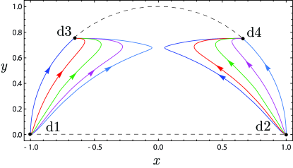
Figure 4: Model II: The phase plane for the DBI dark energy with interaction to dark matter corresponding to $\alpha=1$ for $\tilde{\lambda}_{1}=1$, $\tilde{\gamma}=0$. The late-time attractors, (d3) and (d4), are stable fixed points which lead to accelerated expansion.

For the “nonrelativistic” (i.e., $\tilde{\gamma}=1$) fixed points (e1) and (e2), $\mu_{1}$ is always positive, whereas $\mu_{2}$ can be either positive or negative depending on the value of $\alpha$. If $\alpha<-3$ then $\mu_{2}<0$ and (e1) and (e2) are saddle points. If $\alpha>-3$, then $\mu_{2}>0$ and (e1) and (e2) are unstable fixed points. For the points (e3) and (e4), $\mu_{1}$ and $\mu_{2}$ can be either positive or negative depending on the value of $\alpha$. These points are stable for $\alpha>3$, are saddle points for $-3\leq\alpha\leq 3$, and are unstable nodes for $\alpha<-3$. Thus none of the points (e1) - (e4) are stable, and from Table 4 none of these fixed points lead to accelerated expansion. Thus all of these points are not phenomenologically viable.

Only points (d3) and (d4) satisfy the criteria of accelerated expansion (for values of $\tilde{\lambda}_{1}<2$) and stability (for certain values of $\alpha$ and $\tilde{\lambda}_{1}$). Here, in contrast to the case for Model I, the coupling between dark energy and dark matter plays a significant role in the stability of the fixed points. Although fixed points (d3) and (d4) would still exist without the coupling between dark energy and dark matter characterized by the parameter $\alpha$, the stability of these points does depend crucially on $\alpha$ and therefore on the coupling between dark energy and dark matter. From Table 4 one can see that if one sets $\tilde{\lambda}_{1}=2$ (i.e., the maximum value for which one still gets accelerated expansion), then $\alpha$ is restricted as

$$2\alpha+\sqrt{\frac{\alpha^{2}-6\alpha+9}{\alpha}}<10.$$ (32)

Solving this gives the restriction that

$$0.088<\alpha<4.62~{}.$$ (33)

Only for this range of $\alpha$ (and also one needs $\tilde{\lambda}_{1}<2$) does one get both a stable critical point and accelerated expansion.

IV Summary and Conclusions

In this paper we studied the dynamics of dark energy (in the form of a Dirac-Born-Infeld scalar field) interacting with dark matter (in the form of a fluid) in standard, flat FRW cosmology. For the scalar potential and the brane tension of the DBI scalar field we took power-law functions. We analyzed two different models for the interaction between dark energy and dark matter. Starting with the general interaction equation (4) and (5) we considered $Q=\sqrt{2/3}\beta\rho_{m}\dot{\phi}$ (i.e., Model I) and $Q=\alpha H\rho_{m}$ (i.e., Model II). For each model of the dark energy-dark matter interaction we were interested in fixed points which had accelerated expansion (i.e., $w_{eff}<-1/3$) and for which the fixed points were stable.

For Model I, from Tables 1 and 2 one can see that points (a1), (a2), and (b2) satisfy these two conditions. However, none of these points had any dependence on the coupling parameter $\beta$ between the dark energy and dark matter. Thus for Model I there was no effect of adding the coupling between dark energy and dark matter or a model which only had a DBI scalar field. Thus while not ruled out, Model I is not really of interest since the coupling to dark matter does not lead to any different result from simply having a DBI scalar field.

For Model II we find two stable fixed points which have late time acceleration - points (d3) and (d4) - as can be seen in Tables 3 and 4. In addition from Table 4 one can see that whether or not one has accelerated expansion depends on $\tilde{\lambda}_{1}$, which from Eqs. (14) and (15) depends on the scalar field potential and the tension, but does not depend on the coupling between the DBI field and the dark matter fluid. Thus the addition of a coupling between dark energy, in the form of a DBI scalar field and the dark matter fluid does not appear to contribute to the existence of accelerated expansion for points (d3) and (d4) in Model II. A similar conclusion was reached for Model I where the stable fixed points with accelerated expansion did not depend on the parameter $\beta$ which was a measure of the coupling between dark energy and dark matter for this model. However, for Model II one can see, by looking at the “stability” column of Table 4 that whether or not a given fixed point is stable does depend on $\alpha$ and therefore on the coupling between the DBI field and the dark matter fluid. In particular in order for the critical points (d3) and (d4) to lead to accelerated expansion and to be stable one needs to restrict the coupling parameter $\alpha$ between the DBI dark energy and dark matter fluid via Eq. (33).

Although we have only examined two specific types of couplings between dark energy (in the guise of a DBI scalar field) and dark matter, we will tentatively advance some general conclusions about such models:

(i) The existence of fixed points with accelerated expansion does not depend on the coupling between the dark energy and the dark matter. One can make a general argument to support this conclusion. Dark matter will fall off like $[a(t)]^{-3}$, while if the dark energy is to lead to late-time acceleration it will act like a cosmological constant which falls off like $[a(t)]^{0}\rightarrow$ constant. At late times the $[a(t)]^{0}$ behavior will always dominate the $[a(t)]^{-3}$ behavior.

(ii) While the coupling to dark matter does not seem to play a role in the existence of fixed points with accelerated expansion it can play a role in their stability. For example, in Model II the stability of the fixed points (d3) and (d4), which had accelerated expansion, depended on the dark energy-dark matter coupling parameter $\alpha$. However for Model I none of the fixed points’ stability depended on $\beta$, the coupling parameter for this model. Thus it seems that whether coupling between dark energy and dark matter is important to the stability of the fixed points depends crucially on the type of coupling one chooses.

- (1) S. Perlmutter, Ap. J. 517, 565 (1999),
- (2) A.G. Riess, Astron. J. 116, 1009 (1998).
- (3) M. Hicken et al., arXiv:0901.4804 [astro-ph.CO].
- (4) E. Komatsu et al. [WMAP Collaboration], Astrophys. J. Suppl. 180, 330 (2009) [arXiv:0803.0547 [astro-ph]].
- (5) W. J. Percival, S. Cole, D. J. Eisenstein, R. C. Nichol, J. A. Peacock, A. C. Pope and A. S. Szalay, Mon. Not. Roy. Astron. Soc. 381, 1053 (2007) [arXiv:0705.3323 [astro-ph]].
- (6) E. Silverstein and D. Tong, Phys. Rev. D 70, 103505 (2004).
- (7) M. Alishahiha, E. Silverstein and D. Tong, Phys. Rev. D 70, 123505 (2004) [arXiv:hep-th/0404084].
- (8) X. Chen, Phys. Rev. D 71, 063506 (2005) [arXiv:hep-th/0408084].
- (9) X. Chen, JHEP 0508 (2005) 045 [arXiv:hep-th/0501184].
- (10) S. E. Shandera and S. H. Tye, JCAP 0605 (2006) 007 [arXiv:hep-th/0601099].
- (11) B. Gumjudpai and J. Ward, Phys. Rev. D 80 023528 (2009); J. Martin and M. Yamaguchi, Phys. Rev. D 77 123508 (2008).
- (12) C. Armendariz-Picon, T. Damour, and V. F. Mukhanov, Phys. Lett. B458 (1999) 209–218, [hep-th/9904075].
- (13) L. P. Chimento , R. Lazkoz, and I. Sendra, Gen. Relativ. Gravit. DOI:10.1007/s10714-009-0901-z (2009).
- (14) J. E. Lidsey and I. Huston, JCAP 0707 002 (2007); D. Baumann and L. McAllister, Phys. Rev. D 75 123508 (2007).
- (15) Z. K. Guo and N. Ohta, JCAP 0804, 035 (2008) [arXiv:0803.1013 [hep-th]].
- (16) E. J. Copeland, S. Mizuno and M. Shaeri, Phys. Rev. D. 81, 123501 (2010) arXiv:1003.2881v2 [hep-th].
- (17) E. J. Copeland, A. R. Liddle and D. Wands, Phys. Rev. D 57, 4686 (1998) [arXiv:gr-qc/9711068].
- (18) M. Chaves and D. Singleton Mod. Phys. Lett. A 22, 29 (2007)
- (19) E. Guendelman, D. Singleton, and N. Yongram, “A two measure model of dark energy and dark matter”, arXiv:1205.1056.
- (20) M. Quartin, M. O. Calvao, S. E. Joras, R. R. R. Reis, and I. Waga, JCAP 0805, 007 (2008), 0802.0546.; L. P. Chimento, A. S. Jakubi, D. Pavon, andW. Zimdahl, Phys. Rev. D67, 083513 (2003), astro-ph/0303145.; A. P. Billyard and A. A. Coley, Phys. Rev. D61, 083503 (2000), astro-ph/9908224.; J. Valiviita, E. Majerotto, and R. Maartens, JCAP 0807, 020 (2008), 0804.0232.; C. G. Boehmer, G. Caldera-Cabral, R. Lazkoz, and R. Maartens, Phys. Rev. D78, 023505 (2008), 0801.1565.; Z.-K. Guo, N. Ohta, and S. Tsujikawa, Phys. Rev. D76, 023508 (2007), astro-ph/0702015.; C. Wetterich, Astron. Astrophys. 301, 321 (1995), hep11 th/9408025.; L. Amendola, Phys. Rev. D60, 043501 (1999), astroph/ 9904120.; W. Zimdahl and D. Pavon, Phys. Lett. B521, 133 (2001), astro-ph/0105479.; G. R. Farrar and P. J. E. Peebles, Astrophys. J. 604, 1 (2004), astro-ph/0307316.; R.-G. Cai and A. Wang, JCAP 0503, 002 (2005), hepth/ 0411025.; G. Olivares, F. Atrio-Barandela, and D. Pavon, Phys. Rev. D71, 063523 (2005), astro-ph/0503242.; H. M. Sadjadi and M. Alimohammadi, Phys. Rev. D74, 103007 (2006), gr-qc/0610080.; C. Quercellini, M. Bruni, A. Balbi, and D. Pietrobon (2008), 0803.1976.; J.-H. He, B. Wang, and E. Abdalla (2008), 0807.3471.; X.-m. Chen, Y. Gong, and E. N. Saridakis (2008), 0812.1117.; N. Dalal, K. Abazajian, E. E. Jenkins, and A. V. Manohar, Phys. Rev. Lett. 87, 141302 (2001), astroph/ 0105317.; E. Majerotto, D. Sapone, and L. Amendola (2004), astroph/ 0410543.; H. Garcia-Compean, G. Garcia-Jimenez, O. Obregon, and C. Ramirez, JCAP 0807, 016 (2008), 0710.4283.; M. R. Setare and E. C. Vagenas (2007), 0704.2070.; N. J. Nunes and D. F. Mota, Mon. Not. Roy. Astron. Soc. 368, 751 (2006), astro-ph/0409481.
- (21) C. Wetterich, Astron. Astrophys. 301, 321 (1995) [arXiv:hep-th/9408025].
- (22) L. Amendola, Phys. Rev. D 60, 043501 (1999) [arXiv:astro-ph/9904120].
- (23) D. J. Holden and D. Wands, Phys. Rev. D 61, 043506 (2000) [arXiv:gr-qc/9908026].
- (24) G. Huey and B. D. Wandelt, Phys. Rev. D 74, 023519 (2006) [arXiv:astro-ph/0407196]; S. Das, P. S. Corasaniti and J. Khoury, Phys. Rev. D 73, 083509 (2006) [arXiv:astro-ph/0510628].
- (25) R. Bean and J. Magueijo, Phys. Lett. B 517, 177 (2001) [arXiv:astro-ph/0007199]; R. Bean, Phys. Rev. D 64, 123516 (2001) [arXiv:astro-ph/0104464]; L. Amendola, C. Quercellini, D. Tocchini-Valentini and A. Pasqui, Astrophys. J. 583, L53 (2003) [arXiv:astro-ph/0205097]; D. Comelli, M. Pietroni and A. Riotto, Phys. Lett. B 571, 115 (2003) [arXiv:hep-ph/0302080]; G. R. Farrar and P. J. E. Peebles, Astrophys. J. 604, 1 (2004) [arXiv:astro-ph/0307316]; M. B. Hoffman, arXiv:astro-ph/0307350; U. Franca and R. Rosenfeld, Phys. Rev. D 69, 063517 (2004) [arXiv:astro-ph/0308149]; R. Fardon, A. E. Nelson and N. Weiner, JCAP 0410, 005 (2004) [arXiv:astro-ph/0309800]; F. Vernizzi, Phys. Rev. D 69, 083526 (2004) [arXiv:astro-ph/0311167]; X. J. Bi, P. h. Gu, X. l. Wang and X. m. Zhang, Phys. Rev. D 69, 113007 (2004) [arXiv:hep-ph/0311022]; S. Lee, K. A. Olive and M. Pospelov, Phys. Rev. D 70, 083503 (2004) [arXiv:astro-ph/0406039]; A. W. Brookfield, C. van de Bruck, D. F. Mota and D. Tocchini-Valentini, Phys. Rev. Lett. 96, 061301 (2006) [arXiv:astro-ph/0503349]; T. Koivisto, Phys. Rev. D 72, 043516 (2005) [arXiv:astro-ph/0504571]; H. Wei and R. G. Cai, Phys. Rev. D 72, 123507 (2005) [arXiv:astro-ph/0509328]; R. Mainini and S. Bonometto, JCAP 0706, 020 (2007) [arXiv:astro-ph/0703303]; A. Fuzfa and J. M. Alimi, Phys. Rev. D 75 (2007) 123007 [arXiv:astro-ph/0702478]; R. Bean, E. E. Flanagan and M. Trodden, arXiv:0709.1124 [astro-ph]; ibid. arXiv:0709.1128 [astro-ph]; T. Gonzalez and I. Quiros, arXiv:0707.2089 [gr-qc].
- (26) W. Zimdahl and D. Pavon, Phys. Lett. B 521, 133 (2001) [arXiv:astro-ph/0105479]; L. P. Chimento, A. S. Jakubi, D. Pavon and W. Zimdahl, Phys. Rev. D 67, 083513 (2003) [arXiv:astro-ph/0303145]; J. D. Barrow and T. Clifton, Phys. Rev. D 73 (2006) 103520 [arXiv:gr-qc/0604063]; H. M. Sadjadi and M. Alimohammadi, Phys. Rev. D 74, 103007 (2006) [arXiv:gr-qc/0610080].
- (27) Z. K. Guo, N. Ohta and S. Tsujikawa, Phys. Rev. D 76 (2007) 023508 [arXiv:astro-ph/0702015].