A New Continuous-Time Equality-Constrained Optimization Method to Avoid Singularity

Abstract

In equality-constrained optimization, a standard regularity assumption is often associated with feasible point methods, namely the gradients of constraints are linearly independent. In practice, the regularity assumption may be violated. To avoid such a singularity, we propose a new projection matrix, based on which a feasible point method for the continuous-time, equality-constrained optimization problem is developed. First, the equality constraint is transformed into a continuous-time dynamical system with solutions that always satisfy the equality constraint. Then, the singularity is explained in detail and a new projection matrix is proposed to avoid singularity. An update (or say a controller) is subsequently designed to decrease the objective function along the solutions of the transformed system. The invariance principle is applied to analyze the behavior of the solution. We also propose a modified approach for addressing cases in which solutions do not satisfy the equality constraint. Finally, the proposed optimization approaches are applied to two examples to demonstrate its effectiveness.

I Introduction

According to the implementation of a differential equation, most approaches to continuous-time optimization can be classified as either a dynamical system [1],[2],[3] or a neural network [4],[5],[6],[7]. The dynamical system approach relies on the numerical integration of differential equations on a digital computer. Unlike discrete optimazation methods, the step sizes of dynamical system approaches can be controlled automatically in the integration process and can sometimes be made larger than usual. This advantage suggests that the dynamical system approach can in fact be comparable with currently available conventional discrete optimal methods and facilitate faster convergence [1],[3]. The application of a higher-order numerical integration process also enables us to avoid the zigzagging phenomenon, which is often encountered in typical linear extrapolation methods [1]. On the other hand, the neural network approach emphasizes implementation by analog circuits, very large scale integration, and optical technologies [8]. The major breakthrough of this approach is attributed to the seminal work of Hopfield, who introduced an artificial neural network to solve the traveling salesman problem (TSP) [9]. By employing analog hardware, the neural network approach offers low computational complexity and is suitable for parallel implementation.

For continuous-time equality-constrained optimization, existing methods can be classified into three categories [1]: feasible point method (or primal method), augmented function method (or penalty function method), and the Lagrangian multiplier method. Determining whether one method outperforms the others is difficult because each method possesses distinct advantages and disadvantages. Readers can refer to [1],[4],[7],[10] and the references therein for details. The feasible point method directly solves the original problem by searching through the feasible region for the optimal solution. Each point in the process is feasible, and the value of the objective function constantly decreases. Compared with the two other methods, the feasible point method offers three significant advantages that highlight its usefulness as a general procedure that is applicable to almost all nonlinear programming problems [10, p. 360]: i) the terminating point is feasible if the process is terminated before the solution is reached; ii) the limit point of the convergent sequence of solutions must be at least a local constrained minimum; and iii) the approach is applicable to general nonlinear programming problems because it does not rely on special problem structures such as convexity.

In this paper, a continuous-time feasible point approach is proposed for equality-constrained optimization. First, the equality constraint is transformed into a continuous-time dynamical system with solutions that always satisfy the equality constraint. Then, the singularity is explained in detail and a new projection matrix is proposed to avoid singularity. An update (or say a controller) is subsequently designed to decrease the objective function along the solutions of the transformed system. The invariance principle is applied to analyze the behavior of the solution. We also propose a modified approach for addressing cases in which solutions do not satisfy the equality constraint. Finally, the proposed optimization approach is applied to two examples to demonstrate its effectiveness.

Local convergence results do not assume convexity in the optimization problem to be solved. Compared with global optimization methods, local optimization methods are still necessary. First, they often server as a basic component for some global optimizations, such as the branch and bound method [11]. On the other hand, they can require less computation for online optimization. Compared with the discrete optimal methods offered by MATLAB, at least two illustrative examples show that the proposed approach avoids convergence to a singular point and facilitates faster convergence through numerical integration on a digital computer. In view of these, the contributions of this paper are clear and listed as follows.

i) A new projection matrix is proposed to remove a standard regularity assumption that is often associated with feasible point methods, namely that the gradients of constraints are linearly independent, see [1, p.158, Equ.(4)],[2, p.156, Equ.(2.3)],[7, p.1669, Assumption 1]. Compared with a commonly-used modified projection matrix, the proposed projection matrix has better precision. Moreover, its recursive form can be implemented more easily.

ii) Based on the proposed matrix, a continuous-time, equality-constrained optimization method is developed to avoid convergence to a singular point. The invariance principle is applied to analyze the behavior of the solution.

iii) The modified version of the proposed optimization is further developed to address cases in which solutions do not satisfy the equality constraint. This ensures its robustness against uncertainties caused by numerical error or realization by analog hardware.

We use the following notation. $\mathbb{R}^{n}$ is Euclidean space of dimension $n$. $\left\|\mathbf{\cdot}\right\|$ denotes the Euclidean vector norm or induced matrix norm. $I_{n}$ is the identity matrix with dimension $n.$ $0_{n_{1}\times n_{2}}$ denotes a zero vector or a zero matrix with dimension $n_{1}\times n_{2}.$ Direct product $\otimes$ and $\operatorname{vec}\left(\cdot\right)$ operation are defined in Appendix A. The function $\left[\cdot\right]_{\times}:\mathbb{R}^{3}$ $\rightarrow$ $\mathbb{R}^{3\times 3}\$with matrix $H\in\mathbb{R}^{9\times 3}$ is defined in Appendix B. Suppose $g:$ $\mathbb{R}^{n}\rightarrow\mathbb{R}.$ The gradient of the function $g$ is given by $\nabla g\left(x\right)=\nabla_{x}g\left(x\right)=[\partial g\left(x\right)\left/\partial x_{1}\right.$ $\cdots\ \partial g\left(x\right)\left/\partial x_{n}\right.]^{T}\in\mathbb{R}^{n}\$and the matrix of second partial derivatives of $g\left(x\right)$ known as Hessian is given by $\nabla_{xx}$ $:$ $\mathbb{R}$ $\rightarrow$ $\mathbb{R}^{n\times n}$ and $\nabla_{xx}g\left(x\right)=\left[\partial^{2}g\left(x\right)\left/\partial x_{i}\partial x_{j}\right.\right]_{ij}.$

II Problem Formulation

II-A Equality-Constrained Optimization

The class of equality-constrained optimization problems considered here is defined as follows:

$$\underset{x\in\mathbb{R}^{n}}{\min}v\left(x\right),\text{ s.t. }c\left(x\right)=0$$ (1)

where $v:$ $\mathbb{R}^{n}\rightarrow\mathbb{R}$ is the objective function and $c=[c_{1}$ $c_{2}$ $\cdots$ $c_{m}]^{T}\in\mathbb{R}^{m},$ $c_{i}:\mathbb{R}^{n}\rightarrow\mathbb{R}$ are the equality constraints. They are both twice continuously differentiable. Denote by $\nabla c\left(x\right)\triangleq\left[\begin{array}[c]{cccc}\nabla c_{1}\left(x\right)&\nabla c_{2}\left(x\right)&\cdots&\nabla c_{m}\left(x\right)\end{array}\right]\in\mathbb{R}^{n\times m}.$ To avoid a trivial case, suppose the constraint (or feasible set) $\mathcal{F=}\left\{\left.x\in\mathbb{R}^{n}\right|c\left(x\right)=0\right\}\mathcal{\neq\emptyset}$.

Definition 1 [12, pp. 316-317]. For the problem (1), a vector $x^{\ast}\in\mathcal{F}$ is a global minimum if $v\left(x^{\ast}\right)\leq v\left(x\right),$ $\forall x\in\mathcal{F};$ a vector $x^{\ast}\in\mathcal{F}$ is a local (strict local) minimum if there is a neighborhood $\mathcal{N}$ of $x^{\ast}$ such that $v\left(x^{\ast}\right)\leq v\left(x\right)\ (v\left(x^{\ast}\right)<v\left(x\right))$ for $x\in\mathcal{N\cap F}.$

Definition 2 [10, p. 325]. A vector $x^{\ast}\in\mathcal{F}$ is said to be a regular point if the gradient vectors $\nabla c_{1}\left(x^{\ast}\right),\nabla c_{2}\left(x^{\ast}\right),\cdots,\nabla c_{m}\left(x^{\ast}\right)$ are linearly independent. Otherwise, it is called a singular point.

This paper aims to propose an approach to continuous-time, equality-constrained optimization to identify the local minima based on a feedback control perspective.

Remark 1. Inequality-constrained optimizations can be transformed into equality-constrained optimizations by introducing new variables. For example, the inequality constraint $x\leq 1,x\in\mathbb{R}$ can be replaced with an equality constraint $x+z^{2}=1,z\in\mathbb{R}.$ Also, the inequality constraint $-1\leq x\leq 1,x\in\mathbb{R}$ can be replaced with an equality constraint $x=\sin\left(z\right),z\in\mathbb{R}.$ Here, we only focus on equality-constrained optimization.

II-B Equality Constraint Transformation

Optimization problems are often solved by using numerical iterative methods. For an equality-constrained optimization problem, the major difficulty lies in ensuring that each iteration satisfies the constraint and can further move toward the minimum. To address this difficulty, a transformation of the equality constraint is proposed, which is formulated as an assumption.

Assumption 1. For a given $x_{0}\in\mathcal{F},$ there exists a function $f:\mathbb{R}^{n}\rightarrow\mathbb{R}^{n\times l}$ such that

$$\dot{x}\left(t\right)=f\left(x\left(t\right)\right)u\left(t\right),x\left(0\right)=x_{0}$$ (2)

with solutions that satisfy $x\left(t\right)\in\mathcal{F}_{u}\left(x_{0}\right),$ where $\mathcal{F}_{u}\left(x_{0}\right)=\{x\left(t\right)\in\mathcal{F}|\dot{x}\left(t\right)=f\left(x\left(t\right)\right)u\left(t\right),$ $x\left(0\right)=x_{0}\in\mathcal{F},$ $\forall u\left(t\right)\in\mathbb{R}^{l},$ $t\geq 0\}$.

From a feedback control perspective, the update $u$ can be considered as a control input. The objective function $v\left(x\right)$ can be considered a Lyapunov-like function, although $v(x)$ is not required to be a Lyapunov function. Based on Assumption 1, the objective of this paper can be restated as: to design a control input $u$ to decrease $v(x)$ along the solutions of (2) until $x$ has achieved a local minimum. In the following, we will omit the variable $t$ except when necessary.

Remark 2. The proposition of Assumption 1 is motivated by the property of attitude kinematics [13, p. 200]: $\dot{x}=\frac{1}{2}E\left(x\right)w$, where $x=[q_{0}\ q^{T}]^{T}\in\mathbb{R}^{4},$ $q_{0}\in\mathbb{R},\ q,w\in\mathbb{R}^{3}$ and $E\left(x\right)=[-q$ $q_{0}I_{3}+[q]_{\times}^{T}]^{T}\in\mathbb{R}^{4\times 3}.$ The function $\left[\cdot\right]_{\times}:\mathbb{R}^{3}$ $\rightarrow$ $\mathbb{R}^{3\times 3}$ is defined in Appendix B. All solutions of the attitude kinematics satisfy the constraint $\left\|x\right\|^{2}=1$ driven by any $w\in\mathbb{R}^{3}$. The explanation is given as follows. It is easy to check that $x^{T}\dot{x}=\frac{1}{2}x^{T}E\left(x\right)w=0\$since $[q]_{\times}q=0$ for$\ \forall q\in\mathbb{R}^{3}.$ Therefore, the solution always satisfies the constraint $\left\|x\left(t\right)\right\|^{2}=1$ if $\left\|x\left(0\right)\right\|=1,$ $t\geq 0.$ Another representation of attitude kinematics is

$$\dot{R}=\left[w\right]_{\times}R$$ (3)

where $R\in\mathbb{R}^{3\times 3}$ is a rotation matrix satisfying the constraint $R^{T}R=I_{3}$. For (3), we have

$$\frac{d}{dt}\left(R^{T}R\right) =R^{T}\dot{R}+\dot{R}^{T}R$$

$$=R^{T}\left(\left[w\right]_{\times}+\left[w\right]_{\times}^{T}\right)R=0_{3\times 3}.$$

That is why the evolution of $R$ always lies on the constraint $R^{T}R=I_{3}.$

Remark 3. The best choice of $f\left(x\right)$ is to satisfy $\mathcal{F}_{u}\left(x_{0}\right)=\mathcal{F}.$ However, it is difficult to achieve. For example, if $c\left(x\right)=\left(x_{1}+1\right)\left(x_{1}-1\right)$, $x=[x_{1}$ $x_{2}]^{T}\in\mathbb{R}^{2},$ then $\mathcal{F}=\left\{\left.x\in\mathbb{R}^{2}\right|x_{1}=1,x_{1}=-1\right\}$. Since the two sets $\left\{\left.x\in\mathbb{R}^{2}\right|x_{1}=1\right\}$ and $\left\{\left.x\in\mathbb{R}^{2}\right|x_{1}=-1\right\}$ are not connected, the solution of (2) starting from either set cannot access the other. Although $\mathcal{F}_{u}\left(x_{0}\right)\neq\mathcal{F}$, we still expect the global minimum $x^{\ast}\in\mathcal{F}_{u}\left(x_{0}\right).$ That is why we often require that the initial value $x_{0}$ be close to the global minimum $x^{\ast}.$ Besides this, it is also expected that the function $f\left(x\right)$ is chosen to make the set $\mathcal{F}_{u}\left(x_{0}\right)$ as large as possible so that the probability of $x^{\ast}\in\mathcal{F}_{u}\left(x_{0}\right)$ is higher.

If $c\left(x\right)=Ax,$ $A\in\mathbb{R}^{m\times n}$, then the function $f\left(x\right)$ can be chosen to satisfy $\mathcal{F}=\mathcal{F}_{u}\left(x_{0}\right),$ $\forall x_{0}\in\mathcal{F}.$

Theorem 1. Suppose that $c\left(x\right)=Ax$ and $f\left(x\right)=A^{\bot},$ where $A^{\bot}$ is with full column rank, and the space spanned by the columns of $A^{\bot}$ is the null space of $A.$ Then $\mathcal{F}=\mathcal{F}_{u}\left(x_{0}\right),$ $\forall x_{0}\in\mathcal{F}.$

Proof. Since $\mathcal{F}_{u}\left(x_{0}\right)\subseteq\mathcal{F},$ the remaining task is to prove $\mathcal{F}\subseteq\mathcal{F}_{u}\left(x_{0}\right),$ $\forall x_{0}\in\mathcal{F},$ namely for any $\bar{x}\in\mathcal{F}$ there exists a control input $u\in\mathbb{R}^{l}$ that can transfer any initial state $x_{0}\in\mathcal{F}$ to $\bar{x}.$ Since $x_{0},\bar{x}\in\mathcal{F},$ there exist $u_{0},\bar{u}\in\mathbb{R}^{l}$ such that $\bar{x}=A^{\bot}\bar{u}$ and $x\left(0\right)=A^{\bot}u_{0}$ by the definition of $A^{\bot}.$ Design a control input

$$u\left(t\right)=\left\{\begin{array}[c]{c}\frac{1}{\bar{t}}\left(\bar{u}-u_{0}\right),\\ 0,\end{array}\begin{array}[c]{c}0\leq t\leq\bar{t}\\ t>\bar{t}.\end{array}\right..$$

With the control input above, we have

$$x\left(t\right)-x\left(0\right) ={\displaystyle\int\nolimits_{0}^{t}}A^{\bot}u\left(s\right)ds$$

$$={\displaystyle\int\nolimits_{0}^{\bar{t}}}A^{\bot}u\left(s\right)ds=A^{\bot}\bar{u}-A^{\bot}u_{0},$$

when $t\geq\bar{t}$. Then $x\left(t\right)=\bar{x},$ $t\geq\bar{t}.$ Hence $\mathcal{F}\subseteq\mathcal{F}_{u}\left(x_{0}\right),$ $\forall x_{0}\in\mathcal{F}.$ Consequently, $\mathcal{F}=\mathcal{F}_{u}\left(x_{0}\right),$ $\forall x_{0}\in\mathcal{F}.$ $\square$

From the proof of Theorem 1, the choice of $f\left(x\right)$ becomes a controllability problem. However, it is difficult to obtain a controllability condition of a general nonlinear system. Correspondingly, it is difficult to choose $f\left(x\right)$ for a general nonlinear function $c\left(x\right)$ to satisfy $\mathcal{F}=\mathcal{F}_{u}\left(x_{0}\right).$ Motivated by the linear case above, we aim to design a function $f\left(x\right)\$whose range is the null space of $\nabla c\left(x\right)^{T}$ for any fixed $x\in\mathbb{R}^{n}.$ This idea can be formulated as $\mathcal{V}_{1}\left(x\right)=\mathcal{V}_{2}\left(x\right)$, where

$$\mathcal{V}_{1}\left(x\right) =\{z\in\mathbb{R}^{n}|\nabla c\left(x\right)^{T}z=0\},$$

$$\mathcal{V}_{2}\left(x\right) =\{z\in\mathbb{R}^{n}|z=f\left(x\right)u,u\in\mathbb{R}^{l}\}.$$

III Singularity and A New Projection Matrix

III-A Singularity

The function $f$ is the projection matrix, which orthogonally projects a vector onto the null space of $\nabla c^{T}$. One well-known projection matrix is given as follows [1],[2],[7]:

$$f\left(x\right)=I_{n}-\left(\nabla c\left(\nabla c^{T}\nabla c\right)^{-1}\nabla c^{T}\right)\left(x\right).$$ (4)

We can easily verify that $\nabla c\left(x\right)^{T}f\left(x\right)\equiv 0.$ This projection matrix requires that $\nabla c\left(x\right)$ should have full column rank, i.e., every $x\in\mathcal{F}$ is a regular point. However, the assumption does not hold in cases where $\nabla c\left(x\right)^{T}\nabla c\left(x\right)$ is singular. This condition is the major motivation of this paper. For example, consider an equality constraint as

$$c\left(x\right)=\left(x_{1}-x_{2}+2\right)\left(x_{1}+x_{2}\right)=0,$$

where $x=\left[\begin{array}[c]{cc}x_{1}&x_{2}\end{array}\right]^{T}\in\mathbb{R}^{2}.$ The feasible set is either $\left\{\left.x\in\mathbb{R}^{2}\right|x_{1}-x_{2}+2=0\right\}$ or $\left\{\left.x\in\mathbb{R}^{2}\right|x_{1}+x_{2}=0\right\}.$ As shown in Fig.1, the point $x_{p_{1}}=\left[\begin{array}[c]{cc}-2&0\end{array}\right]^{T}$ has a unique feasible direction and the point $x_{p_{2}}=\left[\begin{array}[c]{cc}0&0\end{array}\right]^{T}$ also has a unique feasible direction. Whereas, the point $x_{p_{3}}=\left[\begin{array}[c]{cc}-1&1\end{array}\right]^{T}$ has two feasible directions. This causes the singular phenomena. The singularity often occurs at the intersection of the feasible sets, where exist non-unique feasible directions. Mathematically, $\nabla c\left(x\right)^{T}\nabla c\left(x\right)$ is singular. Concretely, the gradient vector of $c\left(x\right)$ is

$$\nabla c\left(x\right)=\left[\begin{array}[c]{c}2x_{1}+2\\ -2x_{2}+2\end{array}\right].$$

At the points $x_{p_{1}}$ and $x_{p_{2}},$ the gradient vector of $c\left(x\right)$ is

$$\nabla c\left(x_{p_{1}}\right)=\left[\begin{array}[c]{c}-2\\ 2\end{array}\right],\nabla c\left(x_{p_{2}}\right)=\left[\begin{array}[c]{c}2\\ 2\end{array}\right]$$

and by (4), the projection matrices are further

$$f\left(x_{p_{1}}\right)=\left[\begin{array}[c]{cc}0&1\\ 1&0\end{array}\right],f\left(x_{p_{2}}\right)=\left[\begin{array}[c]{cc}0&-1\\ -1&0\end{array}\right]$$

respectively. Whereas, at the point $x_{p_{3}},$ the gradient vector of $c\left(x_{p_{3}}\right)$ is

$$\nabla c\left(x_{p_{3}}\right)=\left[\begin{array}[c]{c}0\\ 0\end{array}\right].$$

For such a case, $\left(\nabla c\left(x_{p_{3}}\right)^{T}\nabla c\left(x_{p_{3}}\right)\right)^{-1}$ does not exist.

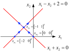
Figure 1: Singularity Example

To avoid singularity, a commonly-used modified projection matrix is given as follows

$$f\left(x\right)=I_{n}-\left(\nabla c\left(\varepsilon I_{m}+\nabla c^{T}\nabla c\right)^{-1}\nabla c^{T}\right)\left(x\right)$$ (5)

where $\varepsilon>0$ is a small positive scale. We have $\nabla c\left(x\right)^{T}f\left(x\right)\neq 0$ no matter how small $\varepsilon$ is. On the other hand, to obtain $f\left(x\right)$ by (5), a very small $\varepsilon$ will cause ill-conditioning problem especially for a low-precision processor. For example, consider the following gradient vectors:

$$\nabla c_{1} =\left[\begin{array}[c]{cccc}1&1&1&1\end{array}\right]$$ (7)

$$\nabla c_{2} =\left[\begin{array}[c]{cccc}2&1&1&1\end{array}\right]$$ (9)

$$\nabla c_{3} =\left[\begin{array}[c]{cccc}3&2&2&2\end{array}\right].$$ (11)

Taking $e_{p}=\left\|\nabla c^{T}f\right\|$ as the precision error, we employ (5) with different $\varepsilon=10^{-k},k=1,\cdots,15$ to obtain the projection matrix $f$. As shown in Fig.2, the error varies with different $k$. The best precision error can be achieved only at $\varepsilon=10^{-8}$ with a precision error around $10^{-8}$. Reducing $\varepsilon$ further will increase the numerical error.

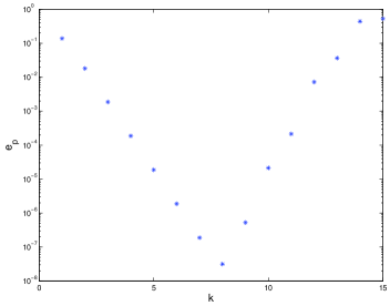
Figure 2: Precision error of a common-used modified projection matrix with different $\varepsilon=10^{-k}$

The best cure is to remove the linearly dependent vector directly from $\nabla c\left(x\right)$. For example, in $\nabla c\left(x\right)=\left[\begin{array}[c]{ccc}\nabla c_{1}\left(x\right)&\nabla c_{2}\left(x\right)&\nabla c_{3}\left(x\right)\end{array}\right]\in\mathbb{R}^{n\times 3}$, if $\nabla c_{3}\left(x\right)$ can be represented by a linear combination of $\nabla c_{1}\left(x\right)\$and $\nabla c_{2}\left(x\right),$ then $\nabla c\left(x\right)^{T}\nabla c\left(x\right)$ is singular. The best cure is to remove $\nabla c_{3}\left(x\right)$ from $\nabla c\left(x\right)$, resulting in

$$\nabla c_{new}\left(x\right)=\left[\begin{array}[c]{cc}\nabla c_{1}\left(x\right)&\nabla c_{2}\left(x\right)\end{array}\right]\in\mathbb{R}^{n\times 2}.$$

With it, the projection matrix becomes

$$f_{new}\left(x\right)=I_{n}-\left(\nabla c_{new}\left(\nabla c_{new}^{T}\nabla c_{new}\right)^{-1}\nabla c_{new}^{T}\right)\left(x\right).$$

It is easy to see that $\nabla c\left(x\right)^{T}f_{new}\left(x\right)\equiv 0.$ For a linear time-invariant matrix $\nabla c\left(x\right),$ namely independent of $x$, we can avoid singularity by removing dependent terms out of $\nabla c\left(x\right)$ before computing a projection matrix. However, this idea does not work for a general $\nabla c\left(x\right)$ depending on $x.$ Therefore, “the best cure” cannot be implemented continuously, which further cannot be realized by analog hardware. For such a purpose, we will propose a new projection matrix.

III-B A New Projection Matrix

For a special case $c:\mathbb{R}^{n}\rightarrow\mathbb{R},$ such a $f\left(x\right)$ is designed in Theorem 2. Consequently, a method is proposed to construct a projection matrix for a general case $c:\mathbb{R}^{n}\rightarrow\mathbb{R}^{m}$. Before the design, we have the following preliminary results.

Lemma 1. Let

$$\mathcal{W}_{1} =\{z\in\mathbb{R}^{n}|L^{T}z=0\}$$

$$\mathcal{W}_{2} =\{z\in\mathbb{R}^{n}|z=\left(I_{n}-\frac{LL^{T}}{\delta\left(\left\|L\right\|^{2}\right)+\left\|L\right\|^{2}}\right)u,u\in\mathbb{R}^{n}\},$$

where $L\in\mathbb{R}^{n}$ and $\delta\left(x\right)=\left\{\begin{array}[c]{c}1\\ 0\end{array}\right.\begin{array}[c]{c}x=0,x\in\mathbb{R}\\ x\neq 0,x\in\mathbb{R}\end{array}.$ Then $\mathcal{W}_{1}=\mathcal{W}_{2}.$

Proof. See Appendix C. $\square$

Theorem 2. Suppose that $c:\mathbb{R}^{n}\rightarrow\mathbb{R}$ and the function $f\left(x\right)$ is designed to be

$$f\left(x\right)=I_{n}-\frac{\nabla c\left(x\right)\nabla c\left(x\right)^{T}}{\delta\left(\left\|\nabla c\left(x\right)\right\|^{2}\right)+\left\|\nabla c\left(x\right)\right\|^{2}}.$$ (12)

Then Assumption 1 is satisfied with $u\in\mathbb{R}^{n}$ and $\mathcal{V}_{1}\left(x\right)=\mathcal{V}_{2}\left(x\right).$

Proof. Since $\dot{c}\left(x\right)=\nabla c\left(x\right)^{T}\dot{x}\$and$\ \dot{x}=f\left(x\right)u$, the function $f\left(x\right)$ is defined as in (12) so that $\dot{c}\left(x\right)\equiv 0$ by Lemma 1. Therefore, Assumption 1 is satisfied with $u\in\mathbb{R}^{n}.$ Further by Lemma 1, $\mathcal{V}_{1}\left(x\right)=\mathcal{V}_{2}\left(x\right).$ $\square$

Theorem 3. Suppose that $c:\mathbb{R}^{n}\rightarrow\mathbb{R}^{m}$ and the function $f\left(x\right)$ is in a recursive form as follows:

$$f_{0} =I_{n}$$

$$f_{k} =f_{k-1}\left(I_{n}-\frac{f_{k-1}^{T}\nabla c_{k}\nabla c_{k}^{T}f_{k-1}}{\delta\left(\left\|f_{k-1}^{T}\nabla c_{k}\right\|^{2}\right)+\left\|f_{k-1}^{T}\nabla c_{k}\right\|^{2}}\right),$$ (13)

$k=1,\cdots,m.$ Then Assumption 1 is satisfied with $f=f_{m}$ and $u\in\mathbb{R}^{n}$ and $\mathcal{V}_{1}\left(x\right)=\mathcal{V}_{2}\left(x\right).$

Proof. See Appendix D. $\square$

Remark 4. In (13), if $\left\|f_{k-1}^{T}\nabla c_{k}\right\|\neq 0,$ then $\delta\left(\left\|f_{k-1}^{T}\nabla c_{k}\right\|^{2}\right)=0,$ namely

$$f_{k}=f_{k-1}\left(I_{n}-\frac{f_{k-1}^{T}\nabla c_{k}\nabla c_{k}^{T}f_{k-1}}{\left\|f_{k-1}^{T}\nabla c_{k}\right\|^{2}}\right).$$

This is the normal way to construct a projection matrix. On the other hand, if $\nabla c_{k}$ can be represented by a linear combination of $\nabla c_{i},$ then $f_{k-1}^{T}\nabla c_{k}=0\$as $f_{k-1}^{T}\nabla c_{i}=0,i=1,\cdots,k-1.$ In this case, $\delta\left(\left\|f_{k-1}^{T}\nabla c_{k}\right\|^{2}\right)\neq 0.$ Consequently, the projection matrix will reduce to the previous one $f_{k}=f_{k-1}$, that is equivalent to removing the term $\nabla c_{k}.$ This is consistent with “the best way”.

Remark 5. In practice, the impulse function $\delta\left(x\right)$ is approximated by some continuous functions such as $\delta\left(x\right)\approx e^{-\gamma\left|x\right|}$, where $\gamma$ is a large positive scale. Let us revisit the example for the gradient vectors (11). Taking $e_{p}=\left\|\nabla c^{T}f\right\|$ as the error again, we employ (13) with $\gamma=30$ to obtain the projection matrix $f$ with $e_{p}=2.7629\ast 10^{-10}.$ This demonstrates the advantage of our proposed projection matrix over (5). Furthermore, compared with (4) or (5), the explicit recursive form of the proposed projection matrix is also easier for the designer to implement.

IV Update Design and Convergence Analysis

In this section, by using Lyapunov’s method, the update (or say controller) $u$ is designed to result in $\dot{v}\left(x\right)\leq 0$. However, the objective function $v\left(x\right)$ is not required to be positive definite. We base our analysis upon the LaSalle invariance theorem [14, pp. 126-129].

IV-A Controller Design

Taking the time derivative of $v\left(x\right)$ along the solutions of (2) results in

$$\dot{v}\left(x\right)=\nabla v\left(x\right)^{T}f\left(x\right)u$$ (14)

where $\nabla v\left(x\right)\in\mathbb{R}^{n}.$ In order to get $\dot{v}\left(x\right)\leq 0,$ a direct way of designing $u$ is proposed as follows

$$u=-Q\left(x\right)f\left(x\right)^{T}\nabla v\left(x\right)$$ (15)

where $Q:\mathbb{R}^{n}\rightarrow\mathbb{R}^{l\times l}$ and $Q\left(x\right)\geq\epsilon I_{l}>0,$ $\epsilon>0,$ $\forall x\in\mathbb{R}^{n}$. Then (14) becomes

$$\dot{v}\left(x\right)=-\nabla v\left(x\right)^{T}f\left(x\right)Q\left(x\right)f\left(x\right)^{T}\nabla v\left(x\right)\leq 0.$$ (16)

Substituting (15) into the continuous-time dynamical system (2) results in

$$\dot{x}=-f\left(x\right)Q\left(x\right)f\left(x\right)^{T}\nabla v\left(x\right)$$ (17)

with solutions which always satisfy the constraint $c\left(x\right)=0.$ The closed-loop system corresponding to the continuous-time dynamical system (2) and the controller (15) is depicted in Fig.3.

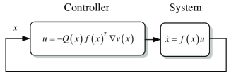
Figure 3: Closed-loop control system

IV-B Convergence Analysis

Unlike a Lyapunov function, the objective function $v\left(x\right)$ is not required to be positive definite. As a consequence, the conclusions for Lyapunov functions are not applicable. Instead, the invariance principle is applied to analyze the behavior of the solution of (17).

Theorem 4. Under Assumption 1, given $x_{0}\in\mathcal{F}$, if the set $\mathcal{K}$ $=$ $\{x\in\mathbb{R}^{n}|v\left(x\right)\leq v\left(x_{0}\right),c\left(x\right)=0\}$ is bounded, then the solution of (17) starting at $x_{0}$ approaches $x_{l}^{\ast}\in\mathcal{S}$, where $\mathcal{S}$ $=$ $\{x\in\mathcal{K}|\nabla v\left(x\right)^{T}f\left(x\right)=0\}.$ If in addition $\mathcal{V}_{1}\left(x_{l}^{\ast}\right)=\mathcal{V}_{2}\left(x_{l}^{\ast}\right),$ then there must exist a $\lambda^{\ast}$ $=$ $[\lambda_{1}^{\ast}\ \lambda_{2}^{\ast}$ $\cdots$ $\lambda_{m}^{\ast}$ $]^{T}$ $\in\mathbb{R}^{m}$ such that $\nabla v\left(x_{l}^{\ast}\right)=\sum_{i=1}^{m}\lambda_{i}^{\ast}\nabla c_{i}\left(x_{l}^{\ast}\right)\$and $c\left(x_{l}^{\ast}\right)=0,$ namely $x_{l}^{\ast}$ is a Karush–Kuhn–Tucker (KKT) point. Furthermore, if $z^{T}\nabla_{xx}L\left(x_{l}^{\ast},\lambda^{\ast}\right)z>0$, for all $z\in\mathcal{V}_{1}\left(x_{l}^{\ast}\right),z\neq 0,$ then $x_{l}^{\ast}$ is a strict local minimum, where $L\left(x,\lambda\right)=v\left(x\right)-\sum_{i=1}^{m}\lambda_{i}c_{i}\left(x\right).$

Proof. The proof is composed of three propositions: Proposition 1 is to show that $\mathcal{K}$ is compact and positively invariant with respect to (17); Proposition 2 is to show that the solution of (17) starting at $x_{0}$ approaches $x_{l}^{\ast}\in\mathcal{S}$; Proposition 3 is to show that $x_{l}^{\ast}\in\mathcal{S}$ is a KKT point, further a strict local minimum. The three propositions are proven in Appendix E. $\square$

Corollary 1. Suppose that $f\left(x\right)$ is chosen as (12) for $c:\mathbb{R}^{n}\rightarrow\mathbb{R}^{m}$ and the set $\mathcal{K}$ $=$ $\{x\in\mathbb{R}^{n}|v\left(x\right)\leq v\left(x_{0}\right),c\left(x\right)=0\}$ is bounded for given $x_{0}\in\mathcal{F}$. Then the solution of (17) starting at $x_{0}$ approaches $x_{l}^{\ast}\in\mathcal{S}$, where $\mathcal{S}$ $=$ $\{x\in\mathcal{K}|\nabla v\left(x\right)^{T}f\left(x\right)=0\},$ where$\ x_{l}^{\ast}$ is a KKT point. In addition, if $z^{T}\nabla_{xx}L\left(x_{l}^{\ast},\lambda^{\ast}\right)z>0$, for all $z\in\mathcal{V}_{1}\left(x_{l}^{\ast}\right),z\neq 0,$ then $x_{l}^{\ast}$ is a strict local minimum, where $L\left(x,\lambda\right)=v\left(x\right)-\sum_{i=1}^{m}\lambda_{i}c_{i}\left(x\right).$

Proof. Since $\mathcal{V}_{1}\left(x_{l}^{\ast}\right)=\mathcal{V}_{2}\left(x_{l}^{\ast}\right)$ by Theorem 3, the remainder of the proof is the same as that of Theorem 4. $\square$

Corollary 2. Consider the following equality-constrained optimization problem

$$\underset{x\in\mathbb{R}^{n}}{\min}v\left(x\right),\text{ s.t. }Ax=b.$$ (18)

If (i) $v\left(x\right)$ is convex and twice continuously differentiable, (ii) $A\in\mathbb{R}^{p\times n}$ with rank$A<n,$ (iii) $\mathcal{K=}\{x\in\mathbb{R}^{n}|v\left(x\right)\leq v\left(x_{0}\right),Ax=b\}$ is bounded, then the solution of (17) with $f\left(x\right)=A^{\bot}$ starting at any $x_{0}\in\mathcal{F}$ approaches $x^{\ast}$.

Proof. The solution of (17) starting at $x_{0}$ approaches $x_{l}^{\ast}\in\mathcal{S}.$ Since rank$A<n,$ we have $\mathcal{V}_{1}\left(x_{l}^{\ast}\right)=\mathcal{V}_{2}\left(x_{l}^{\ast}\right)\neq\varnothing.$ Since the equality constrained optimization problem (18) is convex, a KKT point $x_{l}^{\ast}$ is a global minimum $x^{\ast}$ of the problem (18). The remainder of proof is the same as that of Theorem 4. $\square$

Remark 6. If $\mathcal{K}$ is not a bounded set, then $\mathcal{S}$ defined in Theorem 4 may be empty. Therefore, the boundedness of the set $\mathcal{K}$ is necessary. For example, $v\left(x\right)=x_{1}+x_{2},$ s.t. $c\left(x\right)=x_{1}-x_{2}=0$. The set $\mathcal{K}=\left\{\left.x\in\mathbb{R}^{2}\right|x_{1}+x_{2}\leq v\left(x_{0}\right),x_{1}-x_{2}=0\right\}$ is unbounded. According to Theorem 1, we have $f\left(x\right)=[1$ $1]^{T}.$ In this case, $\nabla v\left(x\right)^{T}f\left(x\right)=2\neq 0\$and then the set $\mathcal{S}$ is empty.

IV-C A Modified Closed-Loop Dynamical System

Although the proposed approach ensures that the solutions satisfy the constraint, this approach may fail if $x_{0}\notin\mathcal{F}$ or if numerical algorithms are used to compute the solutions. Moreover, if the impulse function $\delta$ is approximated, then the constraints will also be violated. With these results, the following modified closed-loop dynamical system is proposed to amend this situation.

Similar to [2], we introduce the term $-\rho\nabla c\left(x\right)c\left(x\right)$ into (17), resulting in

$$\dot{x}=-\rho\nabla c\left(x\right)c\left(x\right)-f\left(x\right)Q\left(x\right)f\left(x\right)^{T}\nabla v\left(x\right),x\left(0\right)=x_{0}$$ (19)

where $\rho>0$. Define $v_{c}\left(x\right)=c\left(x\right)^{T}c\left(x\right).$ Then

$$\dot{v}_{c}\left(x\right)=-\rho c\left(x\right)^{T}\nabla c\left(x\right)^{T}\nabla c\left(x\right)c\left(x\right)\leq 0,$$

where $\nabla c\left(x\right)^{T}f\left(x\right)\equiv 0$ is utilized. If the impulse function $\delta$ is approximated, then $\nabla c\left(x\right)^{T}f\left(x\right)\approx 0$ and can be ignored in practice. Therefore, the solutions of (19) will tend to the feasible set $\mathcal{F}$ if $\nabla c\left(x\right)$ is of full column rank. Once $c\left(x\right)=0,$ the modified dynamical system (19) degenerates to (17). The self-correcting feature enables the step size to be automatically controlled in the numerical integration process or to tolerate uncertainties when the differential equation is realized by using analog hardware.

Remark 7. The matrix $Q\left(x\right)$ plays a role in coordinating the convergence rate of all states by minimizing the condition number of the matrix functions like $f\left(x\right)Q\left(x\right)f\left(x\right)^{T}$. Moreover, it also plays a role in avoiding instability in the numerical solution of differential equations by normalizing the Lipschitz condition of functions like $f\left(x\right)Q\left(x\right)f\left(x\right)^{T}\nabla v\left(x\right).$ Concrete examples are given in the following section.

V Illustrative Examples

V-A Estimate of Attraction Domain

For a given Lyapunov function, the crucial step in any procedure for estimating the attraction domain is determining the optimal estimate. Consider the system of differential equations:

$$\dot{x}=Ax+g\left(x\right)$$ (20)

where $x\in\mathbb{R}^{n}$ is the state vector, $A\in\mathbb{R}^{n\times n}$ is a Hurwitz matrix, and $g:\mathbb{R}^{n}\rightarrow\mathbb{R}^{n}$ is a vector function. Let $v\left(x\right)=x^{T}Px$ be a given quadratic Lyapunov function for the origin of (20), i.e., $P\in\mathbb{R}^{n\times n}$ is a positive-definite matrix such that $A^{T}P+PA<0$. Then the largest ellipsoidal estimate of the attraction domain of the origin can be computed via the following equality-constrained optimization problem [15]:

$$\underset{x\in\mathbb{R}^{n}\backslash\left\{0\right\}}{\min}x^{T}Px\text{ s.t. }x^{T}P\left[Ax+g\left(x\right)\right]=0.$$

Since $\{x\in\mathbb{R}^{n}|x^{T}Px\leq x_{0}^{T}Px_{0}\}$ is bounded, the subset

$$\mathcal{K}=\{x\in\mathbb{R}^{n}|x^{T}Px\leq x_{0}^{T}Px_{0},x^{T}P\left[Ax+g\left(x\right)\right]=0\}$$

is bounded no matter what $g$ is.

For simplicity, consider (20) with $x=[x_{1}$ $x_{2}]^{T}\in\mathbb{R}^{2},$ $A=-I_{2},$ $P=I_{2}$ and $g\left(x\right)=\left(\sigma\left(x\right)+1\right)[x_{1}$ $x_{2}]^{T},$ where $\sigma\left(x\right)=\left(x_{1}+x_{2}+2\right)\left(\left(x_{2}+1\right)-0.1\left(x_{1}+1\right)^{2}\right).$ Then the optimization problem is formulated as

$$\underset{x\in\mathbb{R}^{2}\backslash\left\{0\right\}}{\min}x_{1}^{2}+x_{2}^{2}\text{ s.t. }\left(x_{1}^{2}+x_{2}^{2}\right)\sigma\left(x\right)=0.$$

Since $x\neq 0,$ the problem is further formulated as

$$\underset{x\in\mathbb{R}^{2}}{\min}v\left(x\right)=x_{1}^{2}+x_{2}^{2}\text{ s.t. }\sigma\left(x\right)=0.$$

Then

$$\nabla v\left(x\right) =[2x_{1}2x_{2}]^{T}$$

$$\nabla c\left(x\right) =\left[\begin{array}[c]{c}d_{2}-0.1d_{1}^{2}-0.2d_{1}d_{3}\\ d_{2}-0.1d_{1}^{2}+d_{3}\end{array}\right]$$

$$d_{1} =x_{1}+1,d_{2}=x_{2}+1,d_{3}=x_{1}+x_{2}+2.$$

In this example, we adopt the modified dynamics (19), where $f$ is chosen as (12) with$\ \delta\left(x\right)=e^{-\gamma\left|x\right|},$  and the parameters  are chosen as$\ \gamma=10,\rho=Q=20\left/\left\|\nabla cc-ff^{T}\nabla v\right\|\right..$ We solve the differential equation (19) by using the MATLAB function “ode45” with “variable-step”. Compared with the MATLAB optimal constrained nonlinear multivariate function “fmincon”, we derive the comparisons in Table 1.

TABLE 1. COMPUTED RESULT FOR EXAMPLE 1

Method Initial Point Solution Optimal Value cpu time (sec.) Matlab fmincon [-3 1]$${}^{\text{{\scriptsize T}}} {}^{\text{{\scriptsize T}}} {}^{\text{{\scriptsize T}}} {}^{\text{{\scriptsize T}}} {}^{\text{{\scriptsize T}}} {}^{\text{{\scriptsize T}}} {}^{\text{{\scriptsize T}}} {}^{\text{{\scriptsize T}}} {}^{\text{{\scriptsize T}}} {}^{\text{{\scriptsize T}}} {}^{\text{{\scriptsize T}}} {}^{\text{{\scriptsize T}}}$$ [-1 -1] 2.0000 Not Available New method [-3 1] [0.2062 -0.8546] 0.7729 0.125 Matlab fmincon [2 -4] [-1 -1] 2.0000 Not Available New method [2 -4] [0.2062 -0.8545] 0.7726 0.0940 Matlab fmincon [1 -4] [0.2143 -0.8533] 0.7740 0.2030 New method [1 -4] [0.2056 -0.8550] 0.7733 0.1100 .

The point $x_{s}=[-1$ $-1]^{T}$ is a singular point, at which $\nabla c\left(x_{s}\right)=[0$ $0]^{T}.$ As shown in Table 1, under initial points $[-3$ $1]^{T}\in\mathcal{F}$ and $[2$ $-4]^{T}\in\mathcal{F},$ the MATLAB function fails to find the minimum and stops at the singular point, whereas the proposed approach still finds the minimum. Under initial point $[1$ $-4]^{T}\notin\mathcal{F},$ the proposed approach can still find the minimum, similar to the MATLAB function. Under a different initial value, the evolutions of (19) are shown in Fig.4. As shown, once close to the singular point $[-1$ $-1]^{T}$, the solutions of (19) change direction and then move to the minimum $x_{l}^{\ast}=[0.2061\ -0.8545]^{T}$. Compared with the discrete optimal methods offered by MATLAB, these results show that the proposed approach avoids convergence to a singular point. Moreover, the proposed approach is comparable with currently available conventional discrete optimal methods and facilitates even faster convergence. The latter conclusion is consistent with that proposed in [1],[3].

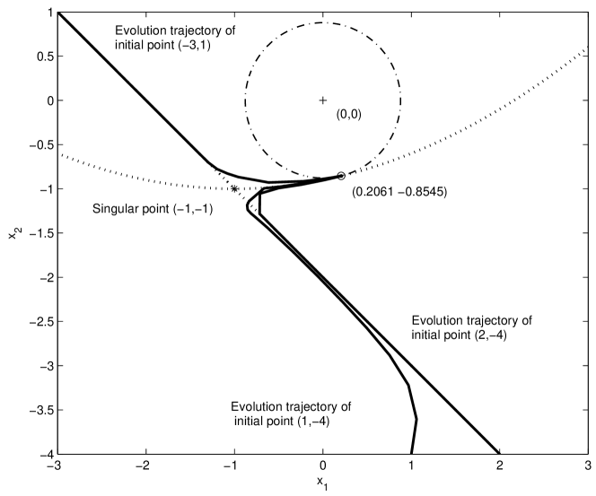
Figure 4: Optimization for estimate of attraction domain. Solution Evolution (solid line), Constraint (dot line), Objective (dash-dot line).

V-B Estimate of Essential Matrix

For simplicity, assume that images are taken by two identical pin-hole cameras with focal length equal to one. The two cameras are specified by the camera centers $C_{1},C_{2}\in\mathbb{R}^{3}$ and attached orthogonal camera frames $\left\{e_{1},e_{2},e_{3}\right\}$ and $\left\{e_{1}^{\prime},e_{2}^{\prime},e_{3}^{\prime}\right\}$, respectively. Denote $T=C_{2}-C_{1}\in\mathbb{R}^{3}$ to be the translation from the first camera to the second and $R\in\mathbb{R}^{3\times 3}$ to be the rotation matrix from the basis vectors $\left\{e_{1},e_{2},e_{3}\right\}$ to $\left\{e_{1}^{\prime},e_{2}^{\prime},e_{3}^{\prime}\right\}$, expressed with respect to the basis $\left\{e_{1},e_{2},e_{3}\right\}.$ Then, it is well known in the computer vision literature [16] that two corresponding image points are represented as follows:

$$m_{1,k} =\frac{1}{M_{k}\left(3\right)}M_{k},$$

$$m_{2,k} =\frac{1}{M_{k}^{\prime}\left(3\right)}M_{k}^{\prime},k=1,2,\cdots,N$$ (21)

where $M_{k},M_{k}^{\prime}$ represent the positions of the $k$th point expressed in the two camera frames $\left\{e_{1},e_{2},e_{3}\right\}$ to $\left\{e_{1}^{\prime},e_{2}^{\prime},e_{3}^{\prime}\right\},$ respectively; $M_{k}\left(3\right),M_{k}^{\prime}\left(3\right)$ represent the third element of vectors $M_{k},M_{k}^{\prime},$ respectively. They have the relationship $M_{k}=RM_{k}^{\prime}+T,$ $k=1,2,\cdots,N.$ These corresponding image points satisfy the socalled epipolar constraint [16, p. 257]:

$$m_{1,k}^{T}Em_{2,k}=0,k=1,2,\cdots,N$$ (22)

where $E=\left[T\right]_{\times}R\$is known as the essential matrix.

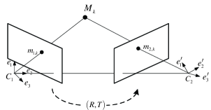
Figure 5: Epipolar geometry

By using the direct product $\otimes$ and the $\operatorname{vec}\left(\cdot\right)$ operation, the equations in (22) are equivalent to

$$A\varphi=0_{N\times 1}$$ (23)

where

$$A =\left[\begin{array}[c]{c}m_{2,1}^{T}\otimes m_{1,1}^{T}\\ \vdots\\ m_{2,N}^{T}\otimes m_{1,N}^{T}\end{array}\right]\in\mathbb{R}^{N\times 9},$$ (27)

$$\varphi =\text{vec}\left(\left[T\right]_{\times}R\right).$$ (28)

In practice, these image points $m_{1,k}$ and $m_{2,k}$ are subject to noise, $k=1,2,\cdots,N$. Therefore, $T$ and $R$ are often solved by the following optimization problem

$$\underset{x\in\mathbb{R}^{12}}{\min}v\left(x\right)=\frac{1}{2}\varphi\left(x\right)^{T}A^{T}A\varphi\left(x\right)$$

$$\text{s.t. }\frac{1}{2}\left(\left\|T\right\|^{2}-1\right)=0$$

$$\text{ \ \ \ \ }\frac{1}{2}\left(R^{T}R-I_{3}\right)=0_{3\times 3}$$ (29)

where $x=[T^{T}$ vec${}^{T}\left(R\right)]^{T}\in\mathbb{R}^{12}$. This is an equality-constrained optimization considered here. In the following, the proposed approach is applied to the optimization problem (29). By Theorem 2, the projection matrix for the constraint $\frac{1}{2}\left(\left\|T\right\|^{2}-1\right)=0$ is

$$f=I_{3}-\frac{TT^{T}}{\delta\left(\left\|T\right\|^{2}\right)+\left\|T\right\|^{2}}.$$

Since $\left\|T\right\|^{2}=1$ has to be satisfied exactly or approximately, then $\delta\left(\left\|T\right\|^{2}\right)=0.$ So, the projection matrix for the constraint is

$$f=I_{3}-T^{T}\left/\left\|T\right\|^{2}\right..$$

Then the constraint is transformed into

$$\dot{T}=\left(I_{3}-TT^{T}\left/\left\|T\right\|^{2}\right.\right)u_{1},$$

where$\ u_{1}\in\mathbb{R}^{3}$. By (3), the constraint $\frac{1}{2}\left(R^{T}R-I_{3}\right)=0_{3\times 3}\$is transformed into

$$\dot{R}=\left[u_{2}\right]_{\times}R,$$

where $u_{2}\in\mathbb{R}^{3}.$ Furthermore, the equation above is rewritten as

$$\text{vec}\left(\dot{R}\right)=\left(R^{T}\otimes I_{3}\right)Hu_{2}.$$

Then the continuous-time dynamical system, whose solutions always satisfy the equality constraints $\frac{1}{2}\left(\left\|T\right\|^{2}-1\right)$ $=$ $0\$and $\frac{1}{2}\left(R^{T}R-I_{3}\right)$ $=$ $0_{3\times 3}$, is expressed as (2) with

$$f\left(x\right) =\left[\begin{array}[c]{cc}I_{3}-TT^{T}\left/\left\|T\right\|^{2}\right.&0_{3\times 3}\\ 0_{9\times 3}&\left(R^{T}\otimes I_{3}\right)H\end{array}\right]\in\mathbb{R}^{12\times 6},$$ (32)

$$u =\left[\begin{array}[c]{c}u_{1}\\ u_{2}\end{array}\right]\in\mathbb{R}^{6}.$$ (35)

If the initial value $\left\|T\left(0\right)\right\|^{2}=1$ and $R\left(0\right)^{T}R\left(0\right)=I_{3},$ then all solutions of (2) satisfy the equality constraints. Since $\nabla v\left(x\right)=[\begin{array}[c]{cc}\left(R^{T}\otimes I_{3}\right)H&I_{3}\otimes\left[T\right]_{\times}\end{array}]^{T}A^{T}A\varphi,$ the time derivative of $v\left(x\right)$ along the solutions of (2) is

$$\dot{v}\left(x\right)=-\varphi^{T}A^{T}A\Theta\left(x\right)^{T}Q\left(x\right)\Theta\left(x\right)A^{T}A\varphi\leq 0,$$

where

$$\Theta\left(x\right)=\left[\begin{array}[c]{c}\left(I_{3}-TT^{T}\left/\left\|T\right\|^{2}\right.\right)^{T}H^{T}\left(R^{T}\otimes I_{3}\right)^{T}\\ H^{T}\left(R^{T}\otimes I_{3}\right)^{T}\left(I_{3}\otimes\left[T\right]_{\times}\right)^{T}\end{array}\right]\in\mathbb{R}^{6\times 9}.$$

The simplest way of choosing $Q\left(x\right)$ is $Q\left(x\right)\equiv I_{6}$. In this case, the eigenvalues of the matrix $A\Theta^{T}\left(x\right)\Theta\left(x\right)A^{T}$ are often ill-conditioned, namely

$$\lambda_{\text{min}}\left(A\Theta^{T}\left(x\right)\Theta\left(x\right)A^{T}\right)\ll\lambda_{\text{max}}\left(A\Theta^{T}\left(x\right)\Theta\left(x\right)A^{T}\right).$$

Convergence rates of the components of $A\varphi\left(x\right)$ depend on the eigenvalues of $A\Theta^{T}\left(x\right)Q\left(x\right)\Theta\left(x\right)A^{T}.$ As a consequence, some components of $A\varphi$ converge fast, while the other may converge slowly. This leads to poor asymptotic performance of the closed-loop system. It is expected that each component of $A\varphi$ can converge at the same speed as far as possible. Suppose that there exists a $\bar{Q}\left(x\right)$ such that

$$A\Theta^{T}\left(x\right)\bar{Q}\left(x\right)\Theta\left(x\right)A^{T}=I_{9}.$$

Then

$$\dot{v}\left(x\right)\leq-\varphi^{T}A^{T}A\varphi\leq 0.$$

By Theorem 4, $x\$will approach the set $\left\{\left.x\in\mathbb{R}^{n}\right|A\varphi\left(x\right)=0\right\},$ each element of which is a global minimum since $v\left(x\right)=0$ in the set. Moreover, each component of $A\varphi$ converges at a similar speed. However, it is difficult to obtain such a $\bar{Q}\left(x\right)$, since the number of degrees of freedom of $\bar{Q}\left(x\right)\in\mathbb{R}^{6\times 6}$ is less than the number of elements of $I_{9}$. A modified way is to make $A\Theta^{T}\left(x\right)Q\left(x\right)\Theta\left(x\right)A^{T}\approx I_{9}.$ A natural choice is proposed as follows

$$Q\left(x\right)=\mu\left(\left(\Theta\left(x\right)A^{T}A\Theta\left(x\right)^{T}\right)^{{\dagger}}+\epsilon I_{6}\right)$$ (36)

where $\mu>0,$ $\left(\Theta\left(x\right)A^{T}A\Theta^{T}\left(x\right)\right)^{{\dagger}}$ denotes the Moore Penrose inverse of $\Theta\left(x\right)A^{T}A\Theta^{T}\left(x\right)$. The matrix $\epsilon I_{6}$ is to make $Q\left(x\right)$ positive definite, where $\epsilon$ is a small positive real. From the procedure above, $\left(\Theta\left(x\right)A^{T}A\Theta^{T}\left(x\right)\right)^{{\dagger}}$ needs to be computed every time. This however will cost much time. A time-saving way is to update $Q\left(x\right)$ at a reasonable interval. Then (17) becomes

$$\dot{x}=-\mu f\left(x\right)\left(\left(\Theta\left(x\right)A^{T}A\Theta\left(x\right)^{T}\right)^{{\dagger}}+\epsilon I_{6}\right)\Theta\left(x\right)A^{T}A\varphi\left(x\right)$$ (37)

where $f\left(x\right)$ is defined in (35). The differential equation can be solved by Runge-Kutta methods, etc. The solutions of (37) satisfy the constraints, where $x=[T^{T}$ vec$\left(R\right)^{T}]^{T}.$ Moreover, the dynamic system will reach some final resting state eventually.

Suppose that there exist 6 points in the field of view, whose positions are expressed in the first camera frame as follows: $M_{1}=[-1$ $1$ $1]^{T},$ $M_{2}=[2$ $0$ $1]^{T},$ $M_{3}=[1$ $-1$ $1]^{T},$ $M_{4}=[-1$ $-1$ $1]^{T},$ $M_{5}=[1$ $1$ $1]^{T},$ $M_{6}=[-1$ $3$ $1]^{T}.$ Compared with the first camera frame, the second camera frame has translated and rotated with

$$\bar{T}=\left[\begin{array}[c]{c}1\\ 1\\ -1\end{array}\right],\bar{R}=\left[\begin{array}[c]{ccc}0.9900&-0.0894&0.1088\\ 0.0993&0.9910&-0.0894\\ -0.0998&0.0993&0.9900\end{array}\right].$$

The image points are generated by (21). Using the generated image points, we obtain $A$ by (28). Setting the initial value as follows $T\left(0\right)=[0$ $0$ $1]^{T},$ $R\left(0\right)=I_{3},$ $\mu=20,$ $\epsilon=0.01.$ We solve the differential equation (19) by using MATLAB function “ode45” with “variable-step”. Compared with MATLAB optimal constrained nonlinear multivariate function “fmincon”, we have the following comparisons:

TABLE 2. COMPUTED RESULT FOR EXAMPLE 2

Method $$\left\|R^{\ast T}\bar{R}-I_{3}\right\|$$ cpu time (sec.) MATLAB fmincon 1.2469e-004 0.2500 New Approach 1.8784e-005 0.1400 .

As shown in Table 2, the proposed approach requires less time to achieve a higher accuracy. Given that $v\left(x^{\ast}\right)=0$, the solution is a global minimum. The evolution of each element of $x$ is shown in Fig.5. The state eventually reaches a rest state at a similar speed. With different initial values, several other simulations are also implemented. Based on the results, the proposed algorithm has met the expectations.

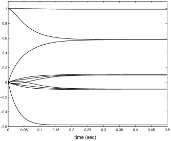
Figure 6: Evolvement of the state

VI Conclusions

An approach to continuous-time, equality-constrained optimization based on a new projection matrix is proposed for the determination of local minima. With the transformation of the equality constraint into a continuous-time dynamical system, the class of equality-constrained optimization is formulated as a control problem. The resultant approach is more general than the existing control theoretic approaches. Thus, the proposed approach serves as a potential bridge between the optimization and control theories. Compared with other standard discrete-time methods, the proposed approach avoids convergence to a singular point and facilitates faster convergence through numerical integration on a digital computer.

Appendix

A. Kronecker Product and Vec

The symbol vec$(X)$ is the column vector obtained by stacking the second column of $X$ under the first, and then the third, and so on. With $X=\left[x_{ij}\right]\in\mathbb{R}^{n\times m}$, the Kronecker product $X\otimes Y$ is the matrix

$$X\otimes Y=\left[\begin{array}[c]{ccc}x_{11}Y&\cdots&x_{1m}Y\\ \vdots&\ddots&\vdots\\ x_{n1}Y&\cdots&x_{nm}Y\end{array}\right].$$

In fact, we have the following relationships vec$(XYZ)=\left(Z^{T}\otimes X\right)$vec$(Y)$ [17, p. 318].

B. Skew-Symmetric Matrix

The cross product of two vectors $x\in\mathbb{R}^{3}$ and $y\in\mathbb{R}^{3}$ is denoted by $x\times y=\left[x\right]_{\times}y,$ where the symbol $\left[\cdot\right]_{\times}:$ $\mathbb{R}^{3}$ $\rightarrow$ $\mathbb{R}^{3\times 3}$ is defined as [13, p. 194]:

$$\left[x\right]_{\times}\triangleq\left[\begin{array}[c]{ccc}0&-x_{3}&x_{2}\\ x_{3}&0&-x_{1}\\ -x_{2}&x_{1}&0\end{array}\right]\in\mathbb{R}^{3\times 3}.$$

By the definition of $\left[x\right]_{\times},$ we have$\ x\times x=\left[x\right]_{\times}x=0_{3\times 1},$ $\forall x\in\mathbb{R}^{3}\$and

$$\text{vec}\left(\left[x\right]_{\times}\right) =Hx,$$

$$H =\left[\begin{array}[c]{ccccccccc}0&0&0&0&0&1&0&-1&0\\ 0&0&-1&0&0&0&1&0&0\\ 0&1&0&-1&0&0&0&0&0\end{array}\right]^{T}.$$

C. Proof of Lemma 1

Since $\delta\left(\left\|L\right\|^{2}\right)+\left\|L\right\|^{2}=1$ if $L=0$ and $\delta\left(\left\|L\right\|^{2}\right)+\left\|L\right\|^{2}=\left\|L\right\|^{2}$ if $L\neq 0,$ we have $\delta\left(\left\|L\right\|^{2}\right)+\left\|L\right\|^{2}\neq 0$, $\forall L\in\mathbb{R}^{n}.$ According to this, we have the following relationship

$$L^{T}\left(I_{n}-LL^{T}\left/\left(\delta\left(\left\|L\right\|^{2}\right)+\left\|L\right\|^{2}\right)\right.\right)$$

$$=L^{T}-L^{T}\left\|L\right\|^{2}\left/\left(\delta\left(\left\|L\right\|^{2}\right)+\left\|L\right\|^{2}\right)\right.$$

$$\equiv 0,\text{ }\forall L\in\mathbb{R}^{n}.$$

This implies that $L^{T}z=0,$ $\forall z\in\mathcal{W}_{2}$, namely $\mathcal{W}_{2}\subseteq\mathcal{W}_{1}$. On the other hand, any $z\in\mathcal{W}_{1}$ is rewritten as

$$z=\left(I_{n}-LL^{T}\left/\left(\delta\left(\left\|L\right\|^{2}\right)+\left\|L\right\|^{2}\right)\right.\right)z$$

where $L^{T}z=0$ is utilized. Hence $\mathcal{W}_{1}\subseteq\mathcal{W}_{2}.$ Consequently, $\mathcal{W}_{1}=\mathcal{W}_{2}.$

D. Proof of Theorem 3

Denote

$$\mathcal{V}_{1}^{j} =\{z\in\mathbb{R}^{n}|\nabla c_{i}^{T}z=0,i=1,\cdots,j,j\leq m\}$$

$$\mathcal{V}_{2}^{j} =\{z\in\mathbb{R}^{n}|z=f_{j}u_{j},u_{j}\in\mathbb{R}^{n},j\leq m\}.$$

First, by Theorem 2, it is easy to see that the conclusions are satisfied with $j=1$. Assume $\mathcal{V}_{1}^{k-1}$ $=$ $\mathcal{V}_{2}^{k-1}$ and then prove that $\mathcal{V}_{1}^{k}$ $=$ $\mathcal{V}_{2}^{k}$ holds. If so, then we can conclude this proof. By $\mathcal{V}_{1}^{k-1}\left(x\right)$ $=$ $\mathcal{V}_{2}^{k-1}\left(x\right),$ we have

$$\mathcal{V}_{1}^{k} =\{z\in\mathbb{R}^{n}|\nabla c_{k}^{T}z=0,z\in\mathcal{V}_{1}^{k-1}\}$$

$$=\{z\in\mathbb{R}^{n}|\nabla c_{k}^{T}z=0,z=f_{k-1}u_{k-1},u_{k-1}\in\mathbb{R}^{n}\}$$

$$=\{z\in\mathbb{R}^{n}|\nabla c_{k}^{T}f_{k-1}u_{k-1}=0,z=f_{k-1}u_{k-1},u_{k-1}\in\mathbb{R}^{n}\}.$$

By Lemma 1, we have

$$\nabla c_{k}^{T}f_{k-1}u_{k-1} =0\Leftrightarrow$$

$$u_{k-1} =\left(I_{n}-\frac{f_{k-1}^{T}\nabla c_{k}\nabla c_{k}^{T}f_{k-1}}{\delta\left(\left\|f_{k-1}^{T}\nabla c_{k}\right\|^{2}\right)+\left\|f_{k-1}^{T}\nabla c_{k}\right\|^{2}}\right)u_{k},$$

namely,

$$\mathcal{V}_{1}^{k}=\mathcal{V}_{2}^{k}=\left\{z\in\mathbb{R}^{n}\left|z=f_{k}u_{k},u_{k}\in\mathbb{R}^{n}\right.\right\}$$

where $f_{k}=f_{k-1}\left(I_{n}-\frac{f_{k-1}^{T}\nabla c_{k}\nabla c_{k}^{T}f_{k-1}}{\delta\left(\left\|f_{k-1}^{T}\nabla c_{k}\right\|^{2}\right)+\left\|f_{k-1}^{T}\nabla c_{k}\right\|^{2}}\right).$

E. Proof of Propositions in Theorem 3

(i) Proof of Proposition 1. In the space $\mathbb{R}^{n},$ the set $\mathcal{K}$ is compact iff it is bounded and closed by Theorem 8.2 in [18, p.41]. Hence, the remainder of work is to prove that $\mathcal{K}$ is closed. Suppose, to the contrary, $\mathcal{K\ }$is not closed. Then there exists a sequence $x\left(t_{n}\right)\in\mathcal{K}\rightarrow p\notin\mathcal{K}$ with $t_{n}\rightarrow\infty.$ Whereas, $v\left(p\right)=\underset{t_{n}\rightarrow\infty}{\lim}v\left(x\left(t_{n}\right)\right)\leq v\left(x_{0}\right)$ and $c\left(p\right)=\underset{t_{n}\rightarrow\infty}{\lim}c\left(x\left(t_{n}\right)\right)=0$ which imply $p\in\mathcal{K}.\$The contradiction implies that $\mathcal{K}$ is closed. Hence, the set $\mathcal{K}$ is compact. By (16), $v\left(x\right)\leq v\left(x_{0}\right)$ with respect to (17), $t\geq 0$. By Assumption 1, all solutions of (17) satisfy $c\left(x\right)=0.$ Therefore, $\mathcal{K}$ is positively invariant with respect to (17).

(ii) Proof of Proposition 2. Since $\mathcal{K}$ is compact and positively invariant with respect to (17), by Theorem 4.4 (invariance principle) in [14, p. 128], the solution of (17) starting at $x_{0}$ approaches $\dot{v}\left(x\right)=0,$ namely $\nabla v\left(x\right)^{T}f\left(x\right)=0.$ In addition, since (17) becomes$\ \dot{x}=0$ in $\mathcal{S}$, the solution approaches a constant vector $x_{l}^{\ast}\in\mathcal{S}.$

(iii) Proof of Proposition 3. Since $\mathcal{V}_{1}\left(x_{l}^{\ast}\right)=\mathcal{V}_{2}\left(x_{l}^{\ast}\right)$ and $x_{l}^{\ast}\in\mathcal{S}$ satisfy the following two equalities

$$\nabla v\left(x_{l}^{\ast}\right)^{T}f\left(x_{l}^{\ast}\right)=0,c\left(x_{l}^{\ast}\right)=0,$$

there exists a $u$ such that $z=f\left(x_{l}^{\ast}\right)u$ for any $z\in\mathcal{V}_{1}\left(x_{l}^{\ast}\right).$ As a consequence, for any $z\in\mathcal{V}_{1}\left(x_{l}^{\ast}\right),$ $\nabla v\left(x_{l}^{\ast}\right)^{T}z=\nabla v\left(x_{l}^{\ast}\right)^{T}f\left(x_{l}^{\ast}\right)u=0.$ There must exist $\lambda_{i}^{\ast}\in\mathbb{R},$ $i=1,\cdots,m$ such that $\nabla v\left(x_{l}^{\ast}\right)=\sum_{i=1}^{m}\lambda_{i}^{\ast}\nabla c_{i}\left(x_{l}^{\ast}\right)$. Otherwise $\exists\bar{z}\in\mathcal{V}_{1}\left(x_{l}^{\ast}\right)$,$\ \nabla v\left(x_{l}^{\ast}\right)^{T}\bar{z}\neq 0.$ Therefore, $x_{l}^{\ast}\in\mathcal{S}$ is a KKT point [12, p.328]. Furthermore, by Theorem 12.6 in [12, p.345], $x_{l}^{\ast}$ is a strict local minimum if $z^{T}\nabla_{xx}L\left(x_{l}^{\ast},\lambda^{\ast}\right)z>0$, for all $z\in\mathcal{V}_{1}\left(x_{l}^{\ast}\right),z\neq 0.$

References

- [1] K. Tanabe, A geometric method in nonlinear programming, Journal of Optimization Theory and Applications. 30(1980) 181–210.
- [2] H. Yamashita, A differential equation approach to nonlinear programming, Mathematical Programming, 18 (1980), 155–168.
- [3] A.A. Brown, M.C. Bartholomew-Biggs, ODE versus SQP methods for constrained optimization, Journal of Optimization Theory and Applications, 62 (1989), 371–386.
- [4] S. Zhang, A.G. Constantinides, Lagrange programming neural networks, IEEE Transactions on Circuits and Systems-II: Analog and Digital Signal Processing, 39 (1992), 441–452.
- [5] Z.-G. Hou, A hierarchical optimization neural network for large-scale dynamic systems, Automatica, 37 (2001), 1931–1940.
- [6] L.-Z. Liao, H. Qi, L. Qi, Neurodynamical optimization, Journal of Global Optimization, 28 (2004), 175–195.
- [7] M.P. Barbarosou, N.G. Maratos, A nonfeasible gradient projection recurrent neural network for equality-constrained optimization problems, IEEE Transactions on Neural Networks, 19 (2008), 1665–1677.
- [8] P.-A. Absi, Computation with continuous-time dynamical systems, in the Grand Challenge in Non-Classical Computation International Workshop, York, United Kingdom, 2005, Apr. 18–19.
- [9] J.J. Hopfield, D.W. Tank, Neural computation of decisions in optimization problems, Biological Cybernetics, 52 (1985), 141–152.
- [10] D.G. Luenberger, Y. Ye, Linear and Nonlinear Programming, third ed., Springer, Boston, 2008.
- [11] E.L. Lawler, D.E. Wood, Branch-and-bound methods: a survey, Operations Research, 14 (1966), 699–719.
- [12] J. Nocedal, S.J. Wright, Numerical Optimization, Springer-Verlag, New York, 1999.
- [13] A. Isidori, L. Marconi, A. Serrani, Robust Autonomous Guidance: An Internal Model-Based Approach, Springer-Verlag, London, 2003.
- [14] H.K. Khalil, Nonlinear Systems, third ed., Prentice-Hall, Upper Saddle River, New York, 2002.
- [15] G. Chesi, A. Garulli, A. Tesi, A. Vicino, Solving quadratic distance problems: an LMI-Based approach, IEEE Transaction on Automatic Control, 48 (2003), 200–212.
- [16] R. Hartley, A. Zisserman, Multiple View Geometry in Computer Vision, second ed., Cambridge University Press, Cambridge, 2003.
- [17] U. Helmke, J.B. Moore, Optimization and Dynamical Systems. Springer-Verlag, 1994.
- [18] F. Morgan, Real Analysis and Applications: Including Fourier Series and the Calculus of Variations. American Mathematical Society, 2005.