Exotic $QQ\bar{q}\bar{q}$, $QQ\bar{q}\bar{s}$, and $QQ\bar{s}\bar{s}$ states

Abstract

After constructing the possible $J^{P}=0^{-},0^{+},1^{-}$, and $1^{+}$ $QQ\bar{q}\bar{q}$ tetraquark interpolating currents in a systematic way, we investigate the two-point correlation functions and extract the corresponding masses with the QCD sum rule approach. We study the $QQ\bar{q}\bar{q}$, $QQ\bar{q}\bar{s}$, and $QQ\bar{s}\bar{s}$ systems with various isospins $I=0,1/2,1$. Our numerical analysis indicates that the masses of doubly bottomed tetraquark states are below the threshold of the two-bottom mesons, two-bottom baryons, and one doubly bottomed baryon plus one antinucleon. Very probably these doubly bottomed tetraquark states are stable.

I Introduction

In the past decade, many charmonium or charmoniumlike states were observed in the B factories, some of which do not fit in the conventional quark model and are considered as the candidates of the exotic states such as molecular states, tetraquark states, hybrid mesons, baryonium states, etc. For experimental reviews of these new states, see Refs. Swanson (2006); Zhu (2008); Bracko (2009); Yuan (2009); Rosner (2007).

Hadronic molecular states are loosely bound states composed of a pair of mesons. They are probably bound by the long-range, color-singlet pion exchange. These interesting states generally lie very close to the open-charm/bottom threshold. Some near-threshold charmoniumlike states such as X(3872) and Z(4430) are very good candidates of the molecular states composed of a pair of charmed and anticharmed mesons. In fact, such a possibility was studied extensively in Refs. Liu et al. (2009, 2008); Swanson (2004a, b); Close and Page (2004); Thomas and Close (2008); Fernandez-Carames et al. (2009).

Tetraquarks are composed of four quarks. They are bound by colored force between quarks. They decay through rearrangement. Some are charged. Some carry strangeness. There are many states within the same multiplet. The low-lying scalar mesons below 1 GeV have been considered good candidates of the tetraquark states. Some of the recently observed charmoniumlike states were also suggested to be candidates of the hidden-charm tetraquark states  Matheus et al. (2007); Maiani et al. (2007); Ebert et al. (2006); Chen and Zhu (2011, 2010); Du et al. (2012); Jiao et al. (2009). We have studied the possible pseudoscalar, scalar, vector, and axial-vector hidden-charm/bottom tetraquark states systematically in the framework of the QCD sum rule Chen and Zhu (2011, 2010); Du et al. (2012); Jiao et al. (2009).

Besides the hidden-charm/bottom $Q{\bar{Q}}q\bar{q}$-type tetraquark states, the doubly-charmed/bottomed tetraquark states $QQ\bar{q}\bar{q}$ are also very interesting, where Q denotes a heavy quark (beauty or charm) and q denotes one light quark (up, down, strange). Such a four-quark configuration is allowed in QCD. In QED we have the hydrogen atom. One light electron circles around the proton. When two electrons are shared by two protons, a hydrogen molecule is formed. In QCD we have the heavy meson. One light antiquark circles around the heavy quark. If the two light antiquarks were shared by the two heavy quarks in the doubly charmed/bottomed tetraquark system, we would have the QCD analogue of the hydrogen molecule!

On the other hand, if the heavy quark QQ pair is spatially close, it would act as a pointlike antiheavy quark color source $\bar{Q}$ and pick up two light quarks $\bar{q}\bar{q}$ to form the bound state $QQ\bar{q}\bar{q}$. The existence and stability of such systems have been studied in many different models, such as the MIT bag model Carlson et al. (1988), chiral quark model Zhang et al. (2008); Pepin et al. (1997), constituent quark model Vijande et al. (2006, 2009); Brink and Stancu (1998); Silvestre-Brac and Semay (1993); Zouzou et al. (1986), and chiral perturbation theory Manohar and Wise (1993). Some other useful references are Navarra et al. (2007); Cui et al. (2007); Gelman and Nussinov (2003); Moinester (1996); Bander and Subbaraman (1994); Ader et al. (1982); Richard (1991); Lipkin (1986, 1973); Carames (2011). However, their existence and stability are model dependent up to now. More theoretical investigations will be helpful in the clarification of the situation.

In this work, we will discuss the $QQ\bar{q}\bar{q}$ systems using the method of QCD sum rule. We first construct the $QQ\bar{q}\bar{q}$ currents with $J^{P}=0^{-}$, $0^{+}$, $1^{-}$, and $1^{+}$ in a systematic way. These currents have no definite C parity due to their special flavor structures. The isospins of these currents can be $I=0,1/2,1$ with specific quark contents. With the independent currents, we investigate the two-point correlation functions and spectral densities. After performing the QCD sum rule analysis, we extract the masses of the possible $0^{-}$, $0^{+}$, $1^{-}$, $1^{+}$ $QQ\bar{q}\bar{q}$, $QQ\bar{q}\bar{s}$, and $QQ\bar{s}\bar{s}$ states.

The paper is organized as follows. In Sec. II, we construct the $QQ\bar{q}\bar{q}$ currents with $J^{P}=0^{-}$, $0^{+}$, $1^{-}$, and $1^{+}$. In Sec. III, we calculate the correlation functions with the operator product expansion(OPE) method and extract the spectral densities. The results are collected in Appendix A. In Sec. IV, we perform the numerical analysis and extract the masses of these tetraquark states. We discuss the possible decay patterns of these doubly charmed/bottomed tetraquark states in Sec. V. The last section is a brief summary.

II tetraquark interpolating currents

In this section, we construct the diquark-antidiquark currents with $J^{P}=0^{-},0^{+},1^{-}$, and $1^{+}$ using the same technique in our previous works Chen and Zhu (2011, 2010). One can construct the tetraquark current with the $qq$ basis or $\bar{q}q$ basis, $(qq)(\bar{q}\bar{q})$ or $(\bar{q}q)(\bar{q}q)$. However, they can be related by the Fierz transformation. In this work, we consider the first set. Considering the Lorentz structures, there are five independent diquark fields without derivatives: $q^{T}_{a}Cq_{b}$, $q^{T}_{a}C\gamma_{5}q_{b}$, $q^{T}_{a}C\gamma_{\mu}q_{b}$, $q^{T}_{a}C\gamma_{\mu}\gamma_{5}q_{b}$, and $q^{T}_{a}C\sigma_{\mu\nu}q_{b}$, where a, b are the color indices. Since $q^{T}_{a}C\sigma_{\mu\nu}\gamma_{5}q_{b}$ and $q^{T}_{a}C\sigma_{\mu\nu}q_{b}$ carry different parity, we consider both operators although they are equivalent. These diquark bilinear can be in the symmetric $\mathbf{6}$ representation or antisymmetric $\mathbf{\bar{3}}$ representation in the color and flavor SU(3) space. Considering the Lorentz structures, we list the properties of these diquark operators in Table II.

$q\Gamma q$	$J^{P}$	States	(Flavor, Color)
$q_{a}^{T}C\gamma_{5}q_{b}$	$0^{+}$	${}^{1}S_{0}$	$(\mathbf{6_{f}},\mathbf{6_{c}}),(\mathbf{\bar{3}_{f}},\mathbf{\bar{3}_{c}})$
$q_{a}^{T}Cq_{b}$	$0^{-}$	${}^{3}P_{0}$	$(\mathbf{6_{f}},\mathbf{6_{c}}),(\mathbf{\bar{3}_{f}},\mathbf{\bar{3}_{c}})$
$q_{a}^{T}C\gamma_{\mu}\gamma_{5}q_{b}$	$1^{-}$	${}^{3}P_{1}$	$(\mathbf{6_{f}},\mathbf{6_{c}}),(\mathbf{\bar{3}_{f}},\mathbf{\bar{3}_{c}})$
$q_{a}^{T}C\gamma_{\mu}q_{b}$	$1^{+}$	${}^{3}S_{1}$	$(\mathbf{6_{f}},\mathbf{\bar{3}_{c}}),(\mathbf{\bar{3}_{f}},\mathbf{6_{c}})$
$q_{a}^{T}C\sigma_{\mu\nu}q_{b}$	$\begin{cases}1^{-},&\mbox{for}~{}\mu,\nu=1,2,3\\ 1^{+},&\mbox{for}~{}\mu=0,\nu=1,2,3\end{cases}$	$\begin{matrix}{}^{1}P_{1}\\ {}^{3}S_{1}\end{matrix}$	$(\mathbf{6_{f}},\mathbf{\bar{3}_{c}}),(\mathbf{\bar{3}_{f}},\mathbf{6_{c}})$
$q_{a}^{T}C\sigma_{\mu\nu}\gamma_{5}q_{b}$	$\begin{cases}1^{+},&\mbox{for}~{}\mu,\nu=1,2,3\\ 1^{-},&\mbox{for}~{}\mu=0,\nu=1,2,3\end{cases}$	$\begin{matrix}{}^{3}S_{1}\\ {}^{1}P_{1}\end{matrix}$	$(\mathbf{6_{f}},\mathbf{\bar{3}_{c}}),(\mathbf{\bar{3}_{f}},\mathbf{6_{c}})$

Table 1: Properties of the diquark operators.

Being composed of two quark (antiquark) fields, the diquark (antidiquark) fields should satisfy Fermi statistics. As shown in Table II, the flavor and color structures are entangled for every diquark operator. For example, the flavor and color structures of the scalar diquark operator $q_{a}^{T}C\gamma_{5}q_{b}$ are either $(\mathbf{6_{f}},\mathbf{6_{c}})$ or $(\mathbf{\bar{3}_{f}},\mathbf{\bar{3}_{c}})$. For $QQ\bar{q}\bar{q}$ systems, the heavy quark pair has the symmetric flavor structure $\mathbf{6_{f}}$. Its flavor and color structures are then fixed as $(\mathbf{6_{f}},\mathbf{6_{c}})$. To construct the color singlet $QQ\bar{q}\bar{q}$ currents, the heavy quark pair $QQ$ and the light antiquark pair $\bar{q}\bar{q}$ should have the same color structures.

According to Ref. Chen and Zhu (2011), there are ten color singlet $QQ\bar{q}\bar{q}$ currents with $J^{P}=0^{-}$:

$$\begin{split}S_{\pm}&=Q^{T}_{a}CQ_{b}(\bar{q}_{a}\gamma_{5}C\bar{q}^{T}_{b}\pm\bar{q}_{b}\gamma_{5}C\bar{q}^{T}_{a}),\\ V_{\pm}&=Q^{T}_{a}C\gamma_{5}Q_{b}(\bar{q}_{a}C\bar{q}^{T}_{b}\pm\bar{q}_{b}C\bar{q}^{T}_{a}),\\ T_{\pm}&=Q^{T}_{a}C\sigma_{\mu\nu}Q_{b}(\bar{q}_{a}\sigma^{\mu\nu}\gamma_{5}C\bar{q}^{T}_{b}\pm\bar{q}_{b}\sigma^{\mu\nu}\gamma_{5}C\bar{q}^{T}_{a}),\\ A_{\pm}&=Q^{T}_{a}C\gamma_{\mu}Q_{b}(\bar{q}_{a}\gamma^{\mu}\gamma_{5}C\bar{q}^{T}_{b}\pm\bar{q}_{b}\gamma^{\mu}\gamma_{5}C\bar{q}^{T}_{a}),\\ P_{\pm}&=Q^{T}_{a}C\gamma_{\mu}\gamma_{5}Q_{b}(\bar{q}_{a}\gamma^{\mu}C\bar{q}^{T}_{b}\pm\bar{q}_{b}\gamma^{\mu}C\bar{q}^{T}_{a}).\end{split}$$ (1)

where “+” denotes the symmetric color structure $[\mathbf{6_{c}}]_{QQ}\otimes[\mathbf{\bar{6}_{c}}]_{\bar{q}\bar{q}}$ and “-” denotes the antisymmetric color structure $[\mathbf{\bar{3}_{c}}]_{QQ}\otimes[\mathbf{3_{c}}]_{\bar{q}\bar{q}}$. Due to the symmetry constraint, it’s enough to keep one light diquark piece only in the bracket of Eq. (1) within the calculation. We keep two terms in Eq. (1) to illustrate the color symmetry explicitly.

By considering the symmetric flavor structure for heavy quark pair $QQ$ , only the currents which satisfy the Pauli principle survive. For the pseudoscalar currents in Eq. (1), $S_{+},V_{+},T_{-},A_{-}$, and $P_{+}$ survive and all the other currents vanish. According to Table II, the $QQ\bar{q}\bar{q}$ ($q=u,d$) operators $S_{+},V_{+},T_{-}$ are isovector currents and $A_{-},P_{+}$ are isoscalar currents. Finally, we obtain the following $QQ\bar{q}\bar{q}$ interpolating currents with $J^{P}=0^{-}$, $0^{+}$, $1^{-}$, and $1^{+}$:

• The tetraquark interpolating currents with $J^{P}=0^{-}$ are

  $$\begin{split}\eta_{1}&=Q^{T}_{a}CQ_{b}(\bar{q}_{a}\gamma_{5}C\bar{q}_{b}^{T}+\bar{q}_{b}\gamma_{5}C\bar{q}^{T}_{a}),\\ \eta_{2}&=Q^{T}_{a}C\gamma_{5}Q_{b}(\bar{q}_{a}C\bar{q}_{b}^{T}+\bar{q}_{b}C\bar{q}^{T}_{a}),\\ \eta_{3}&=Q^{T}_{a}C\sigma_{\mu\nu}Q_{b}(\bar{q}_{a}\sigma^{\mu\nu}\gamma_{5}C\bar{q}^{T}_{b}-\bar{q}_{b}\sigma^{\mu\nu}\gamma_{5}C\bar{q}^{T}_{a}),\\ \eta_{4}&=Q^{T}_{a}C\gamma_{\mu}Q_{b}(\bar{q}_{a}\gamma^{\mu}\gamma_{5}C\bar{q}^{T}_{b}-\bar{q}_{b}\gamma^{\mu}\gamma_{5}C\bar{q}^{T}_{a}),\\ \eta_{5}&=Q^{T}_{a}C\gamma_{\mu}\gamma_{5}Q_{b}(\bar{q}_{a}\gamma^{\mu}C\bar{q}^{T}_{b}+\bar{q}_{b}\gamma^{\mu}C\bar{q}^{T}_{a}).\end{split}$$ (2)

  in which $\eta_{1},\eta_{2},\eta_{3}$ are isovector currents with $[\mathbf{\bar{6}_{f}}]_{\bar{q}\bar{q}}$ and $I=1$, $\eta_{4},\eta_{5}$ are isoscalar currents with $[\mathbf{3_{f}}]_{\bar{q}\bar{q}}$ and $I=0$.

• The tetraquark interpolating currents with $J^{P}=0^{+}$ are

  $$\begin{split}\eta_{1}&=Q^{T}_{a}CQ_{b}(\bar{q}_{a}C\bar{q}_{b}^{T}+\bar{q}_{b}C\bar{q}^{T}_{b}),\\ \eta_{2}&=Q^{T}_{a}C\gamma_{5}Q_{b}(\bar{q}_{a}\gamma_{5}C\bar{q}_{b}^{T}+\bar{q}_{b}\gamma_{5}C\bar{q}^{T}_{b}),\\ \eta_{3}&=Q^{T}_{a}C\gamma_{\mu}Q_{b}(\bar{q}_{a}\gamma^{\mu}C\bar{q}_{b}^{T}-\bar{q}_{b}\gamma^{\mu}C\bar{q}^{T}_{b}),\\ \eta_{4}&=Q^{T}_{a}C\gamma_{\mu}\gamma_{5}Q_{b}(\bar{q}_{a}\gamma^{\mu}\gamma_{5}C\bar{q}_{b}^{T}+\bar{q}_{b}\gamma^{\mu}\gamma_{5}C\bar{q}^{T}_{b}),\\ \eta_{5}&=Q^{T}_{a}C\sigma_{\mu\nu}Q_{b}(\bar{q}_{a}\sigma^{\mu\nu}C\bar{q}^{T}_{b}-\bar{q}_{b}\sigma^{\mu\nu}C\bar{q}^{T}_{a}).\end{split}$$ (3)

  and all the scalar interpolating currents are isovector currents with $[\mathbf{\bar{6}_{f}}]_{\bar{q}\bar{q}}$ and $I=1$.

• The tetraquark interpolating currents with $J^{P}=1^{-}$ are

  $$\begin{split}\eta_{1}&=Q^{T}_{a}C\gamma_{\mu}\gamma_{5}Q_{b}(\bar{q}_{a}\gamma_{5}C\bar{q}_{b}^{T}+\bar{q}_{b}\gamma_{5}C\bar{q}^{T}_{a}),\\ \eta_{2}&=Q^{T}_{a}C\gamma_{5}Q_{b}(\bar{q}_{a}\gamma_{\mu}\gamma_{5}C\bar{q}_{b}^{T}+\bar{q}_{b}\gamma_{\mu}\gamma_{5}C\bar{q}_{a}^{T}),\\ \eta_{3}&=Q^{T}_{a}C\sigma_{\mu\nu}Q_{b}(\bar{q}_{a}\gamma^{\nu}C\bar{q}^{T}_{b}-\bar{q}_{b}\gamma^{\nu}C\bar{q}^{T}_{a}),\\ \eta_{4}&=Q^{T}_{a}C\gamma^{\nu}Q_{b}(\bar{q}_{a}\sigma_{\mu\nu}C\bar{q}^{T}_{b}-\bar{q}_{b}\sigma_{\mu\nu}C\bar{q}^{T}_{a}),\\ \eta_{5}&=Q^{T}_{a}C\gamma_{\mu}Q_{b}(\bar{q}_{a}C\bar{q}_{b}^{T}-\bar{q}_{b}C\bar{q}^{T}_{a}),\\ \eta_{6}&=Q^{T}_{a}CQ_{b}(\bar{q}_{a}\gamma_{\mu}C\bar{q}_{b}^{T}+\bar{q}_{b}\gamma_{\mu}C\bar{q}_{a}^{T}),\\ \eta_{7}&=Q^{T}_{a}C\sigma_{\mu\nu}\gamma_{5}Q_{b}(\bar{q}_{a}\gamma^{\nu}\gamma_{5}C\bar{q}^{T}_{b}-\bar{q}_{b}\gamma^{\nu}\gamma_{5}C\bar{q}^{T}_{a}),\\ \eta_{8}&=Q^{T}_{a}C\gamma^{\nu}\gamma_{5}Q_{b}(\bar{q}_{a}\sigma_{\mu\nu}\gamma_{5}C\bar{q}^{T}_{b}+\bar{q}_{b}\sigma_{\mu\nu}\gamma_{5}C\bar{q}^{T}_{a}).\end{split}$$ (4)

  in which $\eta_{1},\eta_{2},\eta_{3},\eta_{4}$ are isovector currents with $[\mathbf{\bar{6}_{f}}]_{\bar{q}\bar{q}}$ and $I=1$, $\eta_{5},\eta_{6},\eta_{7},\eta_{8}$ are isoscalar currents with $[\mathbf{3_{f}}]_{\bar{q}\bar{q}}$ and $I=0$.

• The tetraquark interpolating currents with $J^{P}=1^{+}$ are

  $$\begin{split}\eta_{1}&=Q^{T}_{a}C\gamma_{\mu}\gamma_{5}Q_{b}(\bar{q}_{a}C\bar{q}_{b}^{T}+\bar{q}_{b}C\bar{q}^{T}_{a}),\\ \eta_{2}&=Q^{T}_{a}CQ_{b}(\bar{q}_{a}\gamma_{\mu}\gamma_{5}C\bar{q}_{b}^{T}+\bar{q}_{b}\gamma_{\mu}\gamma_{5}C\bar{q}_{a}^{T}),\\ \eta_{3}&=Q^{T}_{a}C\sigma_{\mu\nu}\gamma_{5}Q_{b}(\bar{q}_{a}\gamma^{\nu}C\bar{q}^{T}_{b}-\bar{q}_{b}\gamma^{\nu}C\bar{q}^{T}_{a}),\\ \eta_{4}&=Q^{T}_{a}C\gamma^{\nu}Q_{b}(\bar{q}_{a}\sigma_{\mu\nu}\gamma_{5}C\bar{q}^{T}_{b}-\bar{q}_{b}\sigma_{\mu\nu}\gamma_{5}C\bar{q}^{T}_{a}),\\ \eta_{5}&=Q^{T}_{a}C\gamma_{\mu}Q_{b}(\bar{q}_{a}\gamma_{5}C\bar{q}_{b}^{T}-\bar{q}_{b}\gamma_{5}C\bar{q}^{T}_{a}),\\ \eta_{6}&=Q^{T}_{a}C\gamma_{5}Q_{b}(\bar{q}_{a}\gamma_{\mu}C\bar{q}_{b}^{T}+\bar{q}_{b}\gamma_{\mu}C\bar{q}_{a}^{T}),\\ \eta_{7}&=Q^{T}_{a}C\sigma_{\mu\nu}Q_{b}(\bar{q}_{a}\gamma^{\nu}\gamma_{5}C\bar{q}^{T}_{b}-\bar{q}_{b}\gamma^{\nu}\gamma_{5}C\bar{q}^{T}_{a}),\\ \eta_{8}&=Q^{T}_{a}C\gamma^{\nu}\gamma_{5}Q_{b}(\bar{q}_{a}\sigma_{\mu\nu}C\bar{q}^{T}_{b}+\bar{q}_{b}\sigma_{\mu\nu}C\bar{q}^{T}_{a}).\end{split}$$ (5)

  in which $\eta_{1},\eta_{2},\eta_{3},\eta_{4}$ are isovector currents with $[\mathbf{\bar{6}_{f}}]_{\bar{q}\bar{q}}$ and $I=1$, $\eta_{5},\eta_{6},\eta_{7},\eta_{8}$ are isoscalar currents with $[\mathbf{3_{f}}]_{\bar{q}\bar{q}}$ and $I=0$.

For the isovector ($I=1$) currents, we do not differentiate the up and down quarks in our analysis and denote them by $q$. However, they should be differentiated for the isoscalar ($I=0$) currents because the flavor structures of the light anti-diquark $\bar{q}\bar{q}$ are antisymmetric. The quark contents are $QQ\bar{u}\bar{d}$ for these currents. For the $QQ\bar{s}\bar{s}$ systems , only the currents with $[\mathbf{\bar{6}_{f}}]_{\bar{q}\bar{q}}$ flavor structures survive. The isospins for these systems are $I=0$. We will also discuss the $QQ\bar{q}\bar{s}$ systems ($I=1/2$) by using all the currents in Eq. (2)$-$(5). We pick up the interpolating currents with different quark contents in Table. II. To calculate the two-point correlation functions, the Wick contractions of the currents for $QQ\bar{u}\bar{d}$ and $QQ\bar{q}\bar{s}$ systems are different from those for the $QQ\bar{q}\bar{q}$ and $QQ\bar{s}\bar{s}$ systems.

Quark Content	$[\bar{q}\bar{q}]_{\mathbf{f}}$	I	$J^{P}=0^{-}$	$J^{P}=0^{+}$	$J^{P}=1^{-}$	$J^{P}=1^{+}$
$QQ\bar{q}\bar{q}$	$\mathbf{\bar{6}_{f}}$	1	$\eta_{1},\eta_{2},\eta_{3}$	$\eta_{1},\eta_{2},\eta_{3},\eta_{4},\eta_{5}$	$\eta_{1},\eta_{2},\eta_{3},\eta_{4}$	$\eta_{1},\eta_{2},\eta_{3},\eta_{4}$
$QQ\bar{s}\bar{s}$	$\mathbf{\bar{6}_{f}}$	0	$\eta_{1},\eta_{2},\eta_{3}$	$\eta_{1},\eta_{2},\eta_{3},\eta_{4},\eta_{5}$	$\eta_{1},\eta_{2},\eta_{3},\eta_{4}$	$\eta_{1},\eta_{2},\eta_{3},\eta_{4}$
$QQ\bar{q}\bar{s}$	$\mathbf{\bar{6}_{f}}$	$1/2$	$\eta_{1},\eta_{2},\eta_{3},$	$\eta_{1},\eta_{2},\eta_{3},\eta_{4},\eta_{5}$	$\eta_{1},\eta_{2},\eta_{3},\eta_{4},$	$\eta_{1},\eta_{2},\eta_{3},\eta_{4},$
	$\mathbf{3_{f}}$		$\eta_{4},\eta_{5}$		$\eta_{5},\eta_{6},\eta_{7},\eta_{8}$	$\eta_{5},\eta_{6},\eta_{7},\eta_{8}$
$QQ\bar{u}\bar{d}$	$\mathbf{3_{f}}$	0	$\eta_{4},\eta_{5}$	$-$	$\eta_{5},\eta_{6},\eta_{7},\eta_{8}$	$\eta_{5},\eta_{6},\eta_{7},\eta_{8}$

Table 2: The quark contents and isospins of the tetraquark currents.

III QCD sum rule

In QCD sum rule Shifman et al. (1979); Reinders et al. (1985); Colangelo (2000), we consider the two-point correlation functions of the interpolation currents. For the scalar and pseudoscalar currents, the two-point correlation functions read

$$\Pi(q^{2})\equiv i\int d^{4}xe^{iqx}\langle 0|T\eta(x)\eta^{\dagger}(0)|0\rangle,$$ (6)

where $\eta(x)$ is the corresponding interpolating current. The two-point correlation functions of the vector and axial-vector currents are

$$\begin{split}\Pi_{\mu\nu}(q^{2})&=i\int d^{4}xe^{iqx}\langle 0|T\eta_{\mu}(x)\eta_{\nu}^{\dagger}(0)|0\rangle\\ &=\Pi(q^{2})(\frac{q_{\mu}q_{\nu}}{q^{2}}-g_{\mu\nu})+\Pi_{0}(q^{2})\frac{q_{\mu}q_{\nu}}{q^{2}}.\end{split}$$ (7)

There are two parts of $\Pi_{\mu\nu}$ with different Lorentz structures because $\eta_{\mu}$ is not a conserved current. $\Pi(q^{2})$ is related to the vector and axial-vector meson, while $\Pi_{0}$ is the scalar and pseudoscalar current polarization function. At the hadron level, we express the correlation function in the form of the dispersion relation with spectral function,

$$\Pi(q^{2})=(q^{2})^{N}\int_{4(m_{q}+m_{Q})^{2}}^{\infty}\frac{\rho(s)}{s^{N}(s-q^{2}-i\varepsilon)}ds+\sum^{N-1}_{n=0}b_{n}(q^{2})^{n},$$ (8)

where

$$\begin{split}\rho(s)\equiv&\sum_{n}\delta(s-m^{2}_{n})\langle 0|\eta|n\rangle\langle n|\eta^{{\dagger}}|0\rangle\\ =&f^{2}_{X}\delta(s-m^{2}_{X})+\mbox{continuum}\;,\end{split}$$ (9)

where $m_{X}$ is the mass of the resonance $X$ and $f_{X}$ is the decay constant of the meson,

$$\begin{split}&\langle 0|\eta|X\rangle=f_{X},\\ &\langle 0|\eta_{\mu}|X\rangle=f_{X}\epsilon_{\mu}^{X},\end{split}$$ (10)

where $\epsilon_{\mu}^{X}$ is the polarization vector of X ($\epsilon^{X}\cdot q=0$).

One can calculate the correlation functions at the quark-gluon level via the operator product expansion(OPE) method. Using the same technique as in Refs. Chen and Zhu (2011, 2010); Du et al. (2012); Albuquerque and Nielsen (2009); Bracco et al. (2009); Matheus et al. (2007), we calculate the Wilson coefficients while the light quark propagator and heavy quark propagator are adopted as

$$\begin{split}iS_{q}^{ab}&=\frac{i\delta^{ab}}{2\pi^{2}x^{4}}\hat{x}+\frac{i}{32\pi^{2}}\frac{\lambda^{n}_{ab}}{2}g_{s}G^{n}_{\mu\nu}\frac{1}{x^{2}}(\sigma^{\mu\nu}\hat{x}+\hat{x}\sigma^{\mu\nu})-\frac{\delta^{ab}}{12}\langle\bar{q}q\rangle\\ &+\frac{\delta^{ab}x^{2}}{192}\langle g_{s}\bar{q}\sigma\cdot Gq\rangle-\frac{m_{q}\delta^{ab}}{4\pi^{2}x^{2}}+\frac{i\delta^{ab}m_{q}\langle\bar{q}q\rangle}{48}\hat{x},\\ iS_{Q}^{ab}&=\frac{i\delta^{ab}}{\hat{p}-m_{Q}}+\frac{i}{4}g_{s}\frac{\lambda^{n}_{ab}}{2}G^{n}_{\mu\nu}\frac{\sigma^{\mu\nu}(\hat{p}+m_{Q})+(\hat{p}+m_{Q})\sigma^{\mu\nu}}{(p^{2}-m_{Q}^{2})^{2}}\\ &+\frac{i\delta^{ab}}{12}\langle g^{2}_{s}GG\rangle m_{Q}\frac{p^{2}+m_{Q}\hat{p}}{(p^{2}-m_{Q}^{2})^{4}},\end{split}$$ (11)

where $\hat{x}=\gamma_{\mu}x^{\mu}$, $\hat{p}=\gamma_{\mu}p^{\mu}$, $\langle\bar{q}g_{s}\sigma\cdot Gq\rangle=\langle g_{s}\bar{q}\sigma^{\mu\nu}G_{\mu\nu}q\rangle$, $\langle g_{s}^{2}GG\rangle=\langle g_{s}^{2}G_{\mu\nu}G^{\mu\nu}\rangle$. The spectral density is obtained with: $\rho(s)=\frac{1}{\pi}\mbox{Im}\Pi(q^{2})$.

In order to suppress the higher-state contributions and remove the subtraction terms in Eq. (8), we perform the Borel transformation to the correlation function,

$$L_{M_{B}}\Pi(p^{2})=\lim_{{-p^{2},n\to\infty\atop-p^{2}/n\equiv M_{B}^{2}}}\frac{1}{n!}(-p^{2})^{n+1}(\frac{d}{dp^{2}})^{n}\Pi(p^{2}).$$ (12)

After performing the Borel transformation and equating the two representations of the correlation function with the quark-hadron duality, we obtain

$$\Pi(M_{B}^{2})=f_{X}^{2}e^{-m_{X}^{2}/M_{B}^{2}}=\int_{4(m_{q}+m_{Q})^{2}}^{s_{0}}dse^{-s/M_{B}^{2}}\rho(s),$$ (13)

where $s_{0}$ is the threshold parameter, and $M_{B}$ is the Borel parameter. We can extract the meson mass $m_{X}$,

$$m_{X}^{2}=\frac{\int_{4(m_{q}+m_{Q})^{2}}^{s_{0}}dse^{-s/M_{B}^{2}}s\rho^{OPE}(s)}{\int_{4(m_{q}+m_{Q})^{2}}^{s_{0}}dse^{-s/M_{B}^{2}}\rho^{OPE}(s)}.$$ (14)

For all the tetraquark currents in Eq. (2)$-$(5), we collect the spectral densities $\rho(s)$ in Appendix A, respectively. We neglect the three-gluon condensate $\langle g_{s}^{3}fGGG\rangle$ because their contribution is negligible.

IV Numerical Analysis

In the QCD sum rule analysis, we use the following values of the parameters Shifman et al. (1979); Nakamura et al. (2010); Eidemuller and Jamin (2001); Jamin and Pich (1999); Jamin et al. (2002) in the chiral limit ($m_{u}=m_{d}=0$):

$$\begin{split}&m_{s}(1\mbox{GeV})=125\pm 20\mbox{MeV},\\ &m_{c}(m_{c})=(1.23\pm 0.09)~{}\mbox{GeV},\\ &m_{b}(m_{b})=(4.2\pm 0.07)~{}\mbox{GeV},\\ &\langle\bar{q}q\rangle=-(0.23\pm 0.03)^{3}~{}\mbox{GeV}^{3},\\ &\langle\bar{s}s\rangle=(0.8\pm 0.1)\langle\bar{q}q\rangle,\\ &\langle\bar{q}g_{s}\sigma\cdot Gq\rangle=-M_{0}^{2}\langle\bar{q}q\rangle,\\ &M_{0}^{2}=(0.8\pm 0.2)~{}\mbox{GeV},\\ &\langle g_{s}^{2}GG\rangle=(0.48\pm 0.14)~{}\mbox{GeV}^{4}.\end{split}$$ (15)

The Borel mass $M_{B}$ and the threshold value $s_{0}$ are two pivotal parameters. Requiring the convergence of the OPE leads to the lower bound $M^{2}_{Bmin}$ of the Borel parameter. In the present work, we require that the most important condensate contribution be less than one fourth of the perturbative term. We require that the pole contribution be larger than $30\%$, which determines the upper bound $M^{2}_{Bmax}$ of the Borel parameter. The pole contribution (PC) is defined as

$$\mbox{PC}=\frac{\int_{0}^{s_{0}}dse^{-s/M_{B}^{2}}\rho(s)}{\int_{0}^{\infty}dse^{-s/M_{B}^{2}}\rho(s)},$$ (16)

which depends on both the Borel mass $M^{2}_{B}$ and the threshold value $s_{0}$. $s_{0}$ is chosen around the region where the variation of $m_{X}$ with $M_{B}$ is minimum in the Borel working region. For a genuine hadron state, the extracted mass from the sum rule analysis is expected to be stable with the reasonable variation of the Borel parameter $M_{B}^{2}$ and threshold $s_{0}$.

For all the isovector $cc\bar{q}\bar{q}$ and isoscalar $cc\bar{u}\bar{d}$ systems, the most important nonperturbative corrections come from the four-quark condensate $\langle\bar{q}q\rangle^{2}$. Both the quark condensate $\langle\bar{q}q\rangle$ and the quark-gluon mixed condensate $\langle\bar{q}g_{s}\sigma\cdot Gq\rangle$ vanish when we let $m_{u}=m_{d}=m_{q}=0$. For the $(I,J^{P})=(1,0^{-})$ $cc\bar{q}\bar{q}$ system, only the interpolating currents $\eta_{1}$ and $\eta_{3}$ lead to a stable mass sum rule after performing the QCD sum rule analysis. In Fig. IV, we show the mass curves of the extracted hadron mass $m_{X}$ with $M_{B}^{2}$ and $s_{0}$ for the current $\eta_{3}$ with $(I,J^{P})=(1,0^{-})$. The variation of $m_{X}$ with the Borel mass $M_{B}$ is very weak around $s_{0}\sim 23$ GeV². For $\eta_{2}$, the stability of the mass curves is much worse and $m_{X}$ grows monotonically with $s_{0}$ and $M_{B}$. The situation is very similar for the $(I,J^{P})=(0,0^{-})$ $cc\bar{s}\bar{s}$ systems. Now we keep the $m_{s}$ related terms in the spectral densities. These terms are very important corrections for the OPE series. The dominant nonperturbative contribution is the quark condensate $\langle\bar{s}s\rangle$ for $\eta_{2}^{s}$ and $\eta_{3}^{s}$. We show the variations of $m_{X^{s}}$ with the Borel mass $M_{B}^{2}$ and threshold parameter $s_{0}$ for the current $\eta_{3}^{s}$ in Fig. IV.

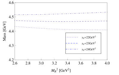
Figure 1: The variation of $m_{X}$ with $M_{B}$ and $s_{0}$ for the current $\eta_{3}$ with $(I,J^{P})=(1,0^{-})$ for $cc\bar{q}\bar{q}$ system.

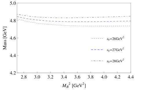
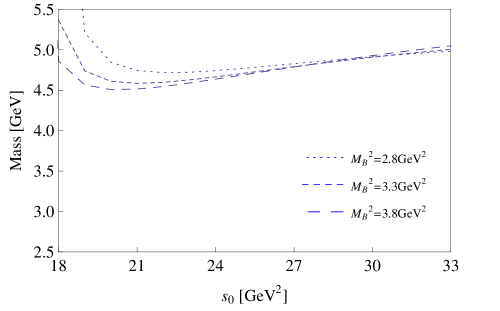
Figure 2: The variation of $m_{X^{s}}$ with $M_{B}$ and $s_{0}$ for the current $\eta_{3}^{s}$ with $(I,J^{P})=(0,0^{-})$ for $cc\bar{s}\bar{s}$ system.

With the parameters in Eq. (15), we list the working region of the Borel parameters, threshold value $s_{0}$, the extracted masses for the currents with $J^{P}=0^{-}$ in Table IV. The pole contribution and the masses are extracted using the corresponding threshold values $s_{0}$ and Borel parameters $M_{B}^{2}$ listed in the table. For the isovector currents $\eta_{1},\eta_{2}$, and $\eta_{3}$, one can also investigate the $QQ\bar{u}\bar{d}$ systems besides the $QQ\bar{u}\bar{u}$ and $QQ\bar{d}\bar{d}$ systems. As mentioned in Sec. II, the Wick contractions of the currents for the $QQ\bar{u}\bar{d}$ systems are different from those for the $QQ\bar{d}\bar{d}$ and $QQ\bar{u}\bar{u}$ systems. However, the correlation functions are the same in the chiral limit ($m_{u}=m_{d}=m_{q}=0$) except for a constant coefficient. We denote them as $QQ\bar{q}\bar{q}$ when we discuss the isovector systems. We take into account the uncertainty of the values of the threshold parameter and variation of the Borel mass to obtain the errors. The other possible error sources are the truncation of the OPE series and the uncertainty of the quark masses. The uncertainty of the condensate values are not included.

Replacing $m_{c}$ with $m_{b}$ in the correlation functions and repeating the same analysis procedures, we obtain the results of the doubly bottomed systems. We also collect the numerical results of the $bb\bar{q}\bar{q}$, $bb\bar{q}\bar{s}$, and $bb\bar{s}\bar{s}$ systems with $J^{P}=0^{-}$ in Table IV.

The derivation and analysis of the QCD sum rules of the $J^{P}=0^{+},1^{-},1^{+}$ $QQ\bar{q}\bar{q}$, $QQ\bar{q}\bar{s}$, and $QQ\bar{s}\bar{s}$ systems are very similar to the $J^{P}=0^{-}$ case. We omit details and collect the numerical results in Table IV, Table IV, and Table IV for the $J^{P}=0^{+},1^{-}$ and $1^{+}$ systems, respectively.

There are no stable sum rules for the $0^{+}$ and $1^{+}$ $cc\bar{q}\bar{q}$ and $cc\bar{u}\bar{d}$ systems. These tetraquarks probably do not exist. The doubly bottomed systems are more stable as the heavy quark mass increases.

In the $J^{P}=1^{+}$ $cc\bar{s}\bar{s}$ system, the extracted mass is about $5.03\sim 5.12$ GeV from the currents $\eta_{1}^{s}$ and $\eta_{2}^{s}$. In contrast, the mass extracted from currents $\eta_{3}^{s}$ and $\eta_{4}^{s}$ is around $4.17$ GeV, which is much lower than that from $\eta_{1}^{s}$ and $\eta_{2}^{s}$. The same situations occur in the $J^{P}=1^{+}$ $cc\bar{q}\bar{s}$, $bb\bar{q}\bar{s}$ and $bb\bar{s}\bar{s}$ cases. According to Table. II, the diquark fields $Q_{a}^{T}C\gamma_{\mu}\gamma_{5}Q_{b}$ and $Q_{a}^{T}CQ_{b}$ are P-wave operators while $Q_{a}^{T}C\gamma_{\mu}Q_{b}$ and $Q_{a}^{T}C\sigma_{\mu\nu}\gamma_{5}Q_{b}$ are S-wave operators. So the interpolating currents $\eta_{1}^{s}$ and $\eta_{2}^{s}$ contain two P-wave operators, whereas $\eta_{3}^{s}$ and $\eta_{4}^{s}$ contain two S-wave operators. In other words, the extracted masses from the currents $\eta_{3}^{s}$ and $\eta_{4}^{s}$ correspond to the ground state mass of the $J^{P}=1^{+}$ $cc\bar{s}\bar{s}$ system while the masses of $\eta_{1}^{s}$ and $\eta_{2}^{s}$ correspond to the orbitally excited state. That is the underlying mechanism which renders the extracted mass from $\eta_{1}^{s}$ and $\eta_{2}^{s}$ is much higher than that from $\eta_{3}^{s}$ and $\eta_{4}^{s}$. The similar situation occurs in the current $\eta_{1}^{s}$ with $J^{P}=0^{+}$ for the $cc\bar{s}\bar{s}$ and $bb\bar{s}\bar{s}$ systems.

There is another intuitive way to understand the difference of the various interpolating currents. According to textbook knowledge about the quark model, the interaction between the quark pair for the symmetric color structure $[\mathbf{6_{c}}]_{QQ}\otimes[\mathbf{\bar{6}_{c}}]_{\bar{q}\bar{q}}$ is repulsive, whereas the interaction for the antisymmetric color structure $[\mathbf{\bar{3}_{c}}]_{QQ}\otimes[\mathbf{3_{c}}]_{\bar{q}\bar{q}}$ is attractive. Thus, the currents with the symmetric color structure will result in higher mass than those with the antisymmetric color structure. There were similar observations of the effect of the color structure on the tetraquark spectrum in Refs. Pepin et al. (1997); Zouzou et al. (1986).

	Current	$s_{0}$	[$M^{2}_{Bmin},M^{2}_{Bmax}$]	$M^{2}_{B}$	$m_{X}$	PC	$f_{X}$	open charm/bottom
		($\mbox{GeV}^{2}$)	($\mbox{GeV}^{2}$)	($\mbox{GeV}^{2}$)	$(\mbox{GeV})$	(%)	($\mbox{GeV}^{5}$)	threshold $(\mbox{GeV})$
$cc\bar{q}\bar{q}$	$\eta_{1}$	24	$3.0\sim 3.9$	3.4	$4.43\pm 0.12$	41.2	0.0674
	$\eta_{3}$	23	$2.6\sim 3.6$	3.1	$4.47\pm 0.12$	42.6	0.312	3.872
$cc\bar{u}\bar{d}$	$\eta_{4}$	22	$2.7\sim 3.4$	3.0	$4.43\pm 0.13$	38.4	0.0870
	$\eta_{5}$	23	$2.5\sim 3.7$	3.2	$4.41\pm 0.14$	41.5	0.106
	$\eta_{1}$	24	$2.9\sim 3.8$	3.4	$4.45\pm 0.16$	40.1	0.0489
	$\eta_{2}$	24	$2.7\sim 3.7$	3.4	$4.68\pm 0.12$	43.1	0.106
$cc\bar{q}\bar{s}$	$\eta_{3}$	26	$3.0\sim 4.4$	3.8	$4.71\pm 0.14$	40.6	0.245	3.975
	$\eta_{4}$	25	$2.6\sim 4.1$	3.4	$4.64\pm 0.13$	44.9	0.136
	$\eta_{5}$	24	$2.6\sim 4.1$	3.4	$4.50\pm 0.16$	45.9	0.124
$cc\bar{s}\bar{s}$	$\eta_{1}$	25	$2.8\sim 4.0$	3.4	$4.46\pm 0.13$	44.3	0.0731	4.081
	$\eta_{3}$	27	$2.7\sim 4.3$	3.4	$4.79\pm 0.17$	47.7	0.558
$bb\bar{q}\bar{q}$	$\eta_{1}$	125	$7.0\sim 9.6$	8.0	$10.6\pm 0.3$	48.6	0.207
	$\eta_{3}$	120	$6.8\sim 9.4$	8.0	$10.5\pm 0.3$	43.7	1.60	10.60
$bb\bar{u}\bar{d}$	$\eta_{5}$	115	$7.0\sim 8.1$	7.5	$10.3\pm 0.2$	36.5	0.367
	$\eta_{1}$	124	$7.2\sim 9.6$	8.5	$10.6\pm 0.2$	40.8	0.188
$bb\bar{q}\bar{s}$	$\eta_{3}$	120	$7.2\sim 9.1$	8.0	$10.6\pm 0.2$	40.2	0.853	10.69
	$\eta_{5}$	115	$7.0\sim 7.9$	7.5	$10.4\pm 0.2$	33.8	0.378
$bb\bar{s}\bar{s}$	$\eta_{1}$	125	$6.7\sim 9.6$	8.0	$10.6\pm 0.3$	47.9	0.286	10.78
	$\eta_{3}$	120	$6.6\sim 8.9$	8.0	$10.6\pm 0.3$	38.0	1.74

Table 3: The numerical results for the doubly-charmed/bottomed $QQ\bar{q}\bar{q}$, $QQ\bar{q}\bar{s}$ and $QQ\bar{s}\bar{s}$ systems with $J^{P}=0^{-}$.

	Current	$s_{0}$	[$M^{2}_{Bmin},M^{2}_{Bmax}$]	$M^{2}_{B}$	$m_{X}$	PC	$f_{X}$	open charm/bottom
		($\mbox{GeV}^{2}$)	($\mbox{GeV}^{2}$)	($\mbox{GeV}^{2}$)	$(\mbox{GeV})$	(%)	($\mbox{GeV}^{5}$)	threshold $(\mbox{GeV})$
$cc\bar{q}\bar{s}$	$\eta_{2}$	22	$2.8\sim 3.6$	3.2	$4.16\pm 0.14$	39.0	0.0548	3.833
	$\eta_{3}$	20	$2.6\sim 3.4$	3.0	$4.02\pm 0.18$	39.3	0.0561
$cc\bar{s}\bar{s}$	$\eta_{1}$	28	$3.2\sim 4.1$	3.4	$5.05\pm 0.15$	43.3	0.136	3.937
	$\eta_{2}$	22	$2.6\sim 3.8$	3.2	$4.27\pm 0.11$	43.2	0.0933
	$\eta_{2}$	120	$7.0\sim 9.8$	8.2	$10.3\pm 0.3$	48.2	0.590
$bb\bar{q}\bar{q}$	$\eta_{3}$	115	$6.9\sim 9.0$	8.0	$10.2\pm 0.3$	40.3	0.539	10.56
	$\eta_{5}$	115	$6.7\sim 8.8$	8.0	$10.2\pm 0.3$	39.4	1.10
	$\eta_{3}$	115	$6.5\sim 8.8$	8.0	$10.2\pm 0.3$	40.3	0.398
$bb\bar{q}\bar{s}$	$\eta_{4}$	115	$5.8\sim 8.6$	7.2	$10.2\pm 0.3$	45.6	0.337	10.65
	$\eta_{5}$	120	$6.2\sim 9.8$	8.0	$10.3\pm 0.3$	49.3	0.806
	$\eta_{1}$	130	$7.5\sim 9.8$	8.5	$11.0\pm 0.2$	41.4	0.391
	$\eta_{2}$	120	$6.4\sim 9.8$	8.0	$10.4\pm 0.3$	49.7	0.632
$bb\bar{s}\bar{s}$	$\eta_{3}$	115	$6.3\sim 9.0$	8.0	$10.2\pm 0.3$	40.5	0.560	10.73
	$\eta_{4}$	120	$6.2\sim 8.4$	8.0	$10.4\pm 0.3$	41.9	0.486
	$\eta_{5}$	115	$6.2\sim 8.8$	8.0	$10.2\pm 0.3$	38.9	1.14

Table 4: The numerical results for the doubly-charmed/bottomed $QQ\bar{q}\bar{q}$, $QQ\bar{q}\bar{s}$ and $QQ\bar{s}\bar{s}$ systems with $J^{P}=0^{+}$.

	Current	$s_{0}$	[$M^{2}_{Bmin},M^{2}_{Bmax}$]	$M^{2}_{B}$	$m_{X}$	PC	$f_{X}$	open charm/bottom
		($\mbox{GeV}^{2}$)	($\mbox{GeV}^{2}$)	($\mbox{GeV}^{2}$)	$(\mbox{GeV})$	(%)	($\mbox{GeV}^{5}$)	threshold $(\mbox{GeV})$
$cc\bar{q}\bar{q}$	$\eta_{1}$	23	$3.0\sim 3.6$	3.3	$4.35\pm 0.14$	38.6	0.0490
$cc\bar{u}\bar{d}$	$\eta_{6}$	23	$3.1\sim 3.7$	3.4	$4.34\pm 0.16$	37.9	0.0395	3.730
	$\eta_{7}$	22	$2.6\sim 3.4$	3.0	$4.41\pm 0.12$	39.4	0.0690
	$\eta_{8}$	23	$2.6\sim 3.5$	3.0	$4.42\pm 0.14$	41.1	0.0940
	$\eta_{1}$	23	$2.7\sim 3.6$	3.2	$4.37\pm 0.17$	39.1	0.0357
	$\eta_{2}$	24	$2.9\sim 3.8$	3.2	$4.59\pm 0.13$	43.0	0.0838
	$\eta_{6}$	23	$2.9\sim 3.7$	3.4	$4.35\pm 0.16$	37.7	0.0353	3.833
$cc\bar{q}\bar{s}$	$\eta_{7}$	24	$2.4\sim 3.9$	3.4	$4.58\pm 0.14$	39.8	0.105
	$\eta_{8}$	24	$2.4\sim 3.9$	3.4	$4.52\pm 0.13$	41.1	0.114
	$\eta_{1}$	24	$2.8\sim 3.7$	3.3	$4.47\pm 0.13$	40.7	0.0603
$cc\bar{s}\bar{s}$	$\eta_{3}$	23	$2.5\sim 3.5$	3.0	$4.47\pm 0.14$	40.9	0.101	3.937
	$\eta_{4}$	26	$2.8\sim 4.2$	3.3	$4.74\pm 0.17$	49.1	0.196
$bb\bar{q}\bar{q}$	$\eta_{1}$	125	$7.0\sim 9.6$	8.0	$10.6\pm 0.3$	47.8	0.229
$bb\bar{u}\bar{d}$	$\eta_{6}$	120	$7.2\sim 8.9$	8.0	$10.4\pm 0.2$	40.5	0.142	10.56
	$\eta_{8}$	120	$8.2\sim 9.4$	8.8	$10.5\pm 0.2$	35.9	0.492
	$\eta_{1}$	120	$7.2\sim 8.8$	8.0	$10.5\pm 0.2$	37.9	0.124
$bb\bar{q}\bar{s}$	$\eta_{6}$	120	$7.2\sim 8.9$	8.0	$10.4\pm 0.2$	40.6	0.145	10.65
	$\eta_{8}$	120	$7.6\sim 9.3$	8.4	$10.5\pm 0.2$	37.8	0.491
	$\eta_{1}$	125	$6.6\sim 9.6$	8.0	$10.6\pm 0.3$	47.1	0.240
$bb\bar{s}\bar{s}$	$\eta_{3}$	120	$6.7\sim 9.0$	8.0	$10.5\pm 0.3$	40.1	0.490	10.73
	$\eta_{4}$	120	$6.8\sim 8.9$	8.0	$10.6\pm 0.3$	38.8	0.655

Table 5: The numerical results for the doubly-charmed/bottomed $QQ\bar{q}\bar{q}$, $QQ\bar{q}\bar{s}$ and $QQ\bar{s}\bar{s}$ systems with $J^{P}=1^{-}$.

	Current	$s_{0}$	[$M^{2}_{Bmin},M^{2}_{Bmax}$]	$M^{2}_{B}$	$m_{X}$	PC	$f_{X}$	open charm/bottom
		($\mbox{GeV}^{2}$)	($\mbox{GeV}^{2}$)	($\mbox{GeV}^{2}$)	$(\mbox{GeV})$	(%)	($\mbox{GeV}^{5}$)	threshold $(\mbox{GeV})$
	$\eta_{1}$	28	$3.0\sim 4.2$	3.6	$4.96\pm 0.11$	42.1	0.0801
	$\eta_{2}$	27	$3.1\sim 4.0$	3.6	$4.87\pm 0.11$	38.5	0.0726
$cc\bar{q}\bar{s}$	$\eta_{3}$	21	$2.4\sim 3.4$	2.8	$4.12\pm 0.17$	47.5	0.0571
	$\eta_{4}$	21	$2.5\sim 3.4$	2.8	$4.13\pm 0.16$	47.9	0.0574	3.975
	$\eta_{5}$	21	$2.8\sim 3.7$	3.2	$4.12\pm 0.16$	41.7	0.0378
	$\eta_{6}$	21	$3.0\sim 3.7$	3.2	$4.17\pm 0.12$	41.5	0.0718
	$\eta_{7}$	21	$2.2\sim 3.3$	2.8	$4.15\pm 0.17$	42.9	0.0465
	$\eta_{1}$	29	$3.2\sim 4.5$	3.8	$5.03\pm 0.13$	42.5	0.138
	$\eta_{2}$	30	$3.2\sim 4.6$	3.8	$5.12\pm 0.14$	45.9	0.150	4.081
$cc\bar{s}\bar{s}$	$\eta_{3}$	21	$2.2\sim 3.4$	2.8	$4.17\pm 0.16$	45.4	0.0838
	$\eta_{4}$	21	$2.2\sim 3.4$	2.8	$4.19\pm 0.16$	45.7	0.0849
$bb\bar{q}\bar{q}$	$\eta_{3}$	115	$6.5\sim 8.8$	7.8	$10.2\pm 0.3$	41.4	0.459
	$\eta_{4}$	115	$6.8\sim 8.8$	7.8	$10.2\pm 0.3$	41.7	0.454
$bb\bar{u}\bar{d}$	$\eta_{5}$	115	$7.0\sim 9.0$	8.0	$10.2\pm 0.3$	42.8	0.215	10.60
	$\eta_{6}$	115	$7.0\sim 9.2$	8.0	$10.2\pm 0.3$	42.0	0.304
	$\eta_{7}$	115	$6.5\sim 8.6$	7.6	$10.2\pm 0.3$	43.2	0.241
	$\eta_{8}$	115	$6.8\sim 8.8$	7.6	$10.2\pm 0.3$	41.7	0.343
	$\eta_{1}$	125	$6.9\sim 8.6$	7.6	$10.7\pm 0.3$	42.1	0.155
	$\eta_{2}$	125	$6.9\sim 8.8$	7.6	$10.7\pm 0.4$	44.5	0.170
$bb\bar{q}\bar{s}$	$\eta_{3}$	120	$6.2\sim 9.8$	8.0	$10.4\pm 0.3$	48.9	0.452
	$\eta_{4}$	120	$6.5\sim 9.8$	8.0	$10.4\pm 0.3$	49.3	0.446	10.69
	$\eta_{5}$	120	$6.6\sim 9.8$	8.0	$10.3\pm 0.3$	52.3	0.298
	$\eta_{6}$	120	$6.6\sim 9.8$	8.0	$10.3\pm 0.4$	52.1	0.418
	$\eta_{7}$	120	$6.2\sim 9.6$	8.0	$10.4\pm 0.3$	48.1	0.342
	$\eta_{8}$	120	$5.8\sim 9.6$	8.0	$10.4\pm 0.3$	46.3	0.491
	$\eta_{1}$	130	$7.0\sim 9.7$	8.5	$11.0\pm 0.3$	40.8	0.336
	$\eta_{2}$	130	$7.2\sim 9.9$	8.5	$10.9\pm 0.3$	42.9	0.370	10.78
$bb\bar{s}\bar{s}$	$\eta_{3}$	120	$6.2\sim 9.8$	8.0	$10.4\pm 0.3$	48.1	0.657
	$\eta_{4}$	120	$6.2\sim 9.8$	8.0	$10.4\pm 0.3$	48.5	0.651

Table 6: The numerical results for the doubly-charmed/bottomed $QQ\bar{q}\bar{q}$, $QQ\bar{q}\bar{s}$ and $QQ\bar{s}\bar{s}$ systems with $J^{P}=1^{+}$.

V Decay Patterns of the $QQ\bar{q}\bar{q}$ and $QQ\bar{s}\bar{s}$ States

In this section, we study the decay patterns of the possible doubly charmed/bottomed states. From the numerical results of Tables IV$-$IV, the extracted masses of the $cc\bar{q}\bar{q}$, $cc\bar{q}\bar{s}$, and $cc\bar{s}\bar{s}$ doubly charmed states are above the $D^{(*)(+/0)}_{(0/1)}D^{(*)(+/0)}_{(0/1)}$, $D^{(*)+}_{(0/1)}D^{(*)+}_{s(0/1)}$, and $D^{(*)+}_{s(0/1)}D^{(*)+}_{s(0/1)}$ thresholds. The possible decay modes of the $cc\bar{q}\bar{q}$, $cc\bar{q}\bar{s}$, and $cc\bar{s}\bar{s}$ states with different quantum numbers are listed in Table V. Both the S-wave and P-wave decay patterns are allowed. These $cc\bar{q}\bar{q}$, $cc\bar{q}\bar{s}$, and $cc\bar{s}\bar{s}$ tetraquarks will decay easily through rearrangement or the so-called fall-apart mechanism. They are very broad resonances. It may be difficult to observe them experimentally.

The situation is very different for the doubly bottomed states. As we emphasize in the previous section, the $\eta_{1}^{s}$ current with $J^{P}=0^{+}$ and the $\eta_{1}^{s},\eta_{2}^{s}$ currents with $J^{P}=1^{+}$ explore the excited tetraquark states because of their special diquark structure. We focus on the doubly bottomed ground states. The extracted masses of these states as shown in Tables IV$-$IV are lower than the open bottom thresholds $\bar{B^{0}}\bar{B^{0}}=10.56$ GeV and $\bar{B^{0}_{s}}\bar{B^{0}_{s}}=10.73$ GeV. These doubly bottomed states cannot decay into the two $b\bar{q}$ or $b\bar{s}$ mesons, which implies the existence of the doubly bottomed bound states $bb\bar{q}\bar{q}$ and $bb\bar{s}\bar{s}$. This observation is consistent with the conclusions of Refs. Carlson et al. (1988); Manohar and Wise (1993); Zhang et al. (2008).

$J^{P}$	S-wave	P-wave
	$D^{0}+D_{0}^{*}(2400)^{0}$,$D^{+}+D_{0}^{*}(2400)^{0}$,	$D^{0}+D^{*}(2007)^{0}$,$D^{+}+D^{*}(2007)^{0}$, $D^{0}+D^{*}(2010)^{+}$,
$0^{-}$	$D^{0}+D_{s0}^{*}(2317)^{+}$,$D^{+}+D_{s0}^{*}(2317)^{+}$,	$D^{+}+D^{*}(2010)^{+}$, $D^{*}(2007)^{0}+D^{*}(2007)^{0}$,
	$D_{0}^{*}(2400)^{0}+D_{s}^{+}$,$D^{*}(2007)^{0}+D_{s1}^{+}$,	$D^{*}(2010)^{+}+D^{*}(2010)^{+}$,$D^{*}(2007)^{0}+D^{*}(2010)^{+}$,
	$D_{1}(2420)^{0}+D^{*}_{s}(2112)^{+}$,$D_{s0}^{*}(2317)^{+}+D_{s}^{+}$,	$D^{*}(2007)^{0}+D^{+}_{s}$,$D^{*}(2010)^{+}+D^{+}_{s}$,$D^{+}+D^{*}_{s}(2112)^{+}$
	…	$D^{+}_{s}+D^{*}_{s}(2112)^{+}$,$D^{*}_{s}(2112)^{+}+D^{*}_{s}(2112)^{+}$,…
	$D^{+}+D_{s}^{+}$,$D^{0}+D_{s}^{+}$,$D_{s}^{+}+D_{s}^{+}$,	$D_{s0}^{*}(2317)^{+}+D^{*}_{s}(2112)^{+}$,
$0^{+}$	$D_{s}^{*+}+D_{s}^{*+}$,$D_{s0}^{*+}+D_{s0}^{*+}$,	$D_{s}^{+}+D_{s1}(2460)^{+}$,$D_{s}^{+}+D_{s1}(2536)^{+}$,
	$D_{s1}^{+}(2460)+D_{s1}^{+}(2460)$,…	…
	$D^{0}+D_{1}^{0}$,$D^{+}+D_{1}^{0}$,	$D^{0}+D^{0}$,$D^{+}+D^{+}$,$D^{0}+D^{+}$,$D^{*0}+D^{*0}$,$D^{*+}+D^{*+}$,
$1^{-}$	$D^{*0}+D_{s0}^{*+}$,$D^{*+}+D_{s0}^{*+}$,	$D^{0}+D^{*0}$,$D^{0}+D^{*+}$,$D^{+}+D^{*0}$,$D^{+}+D^{*+}$,
	$D_{s}^{+}+D_{s1}^{+}$,	$D^{+}+D_{s}^{*+}$,$D^{0}+D_{s}^{*+}$,$D^{*0}+D_{s}^{+}$,$D^{*+}+D_{s}^{+}$,
	…	$D_{s}^{+}+D_{s}^{+}$,$D_{s}^{*+}+D_{s}^{*+}$,…
	$D^{+}+D^{*+}_{s}$,$D^{0}+D^{*+}_{s}$,$D^{*0}+D_{s}^{+}$,	$D^{0}+D_{s0}^{*+}$,$D^{+}+D_{s0}^{*+}$,$D_{0}^{*0}+D_{s}^{+}$,
	$D^{*+}+D_{s}^{+}$,$D_{s}^{+}+D^{*+}_{s}$,	$D^{*0}+D_{s1}^{+}$,$D^{*+}+D_{s1}^{+}$,$D_{1}^{0}+D^{*+}_{s}$,
$1^{+}$	$D_{s0}^{*+}+D_{s1}^{+}$,$D_{s0}^{*+}+D_{s1}^{+}$,$D_{s1}^{+}+D_{s1}^{+}$,…	$D_{s}^{+}+D_{s0}^{*+}$, $D_{s0}^{*+}+D^{*+}_{s}$,$D_{s}^{+}+D_{s1}^{+}$, $D_{s}^{+}+D_{s1}^{+}$,…

Table 7: The possible two-meson decay modes of the $cc\bar{q}\bar{q}$ and $cc\bar{s}\bar{s}$ states.

Except for the two-meson decay modes, these doubly charmed/bottomed tetraquark states may also decay into the two-baryon final states: a pair of bottom and antibottom baryons or one doubly bottomed baryon plus one antinucleon. The lightest bottom baryon is $\Lambda_{b}$. Its mass is 5.62 GeV. In other words, these doubly bottomed tetraquark states do not decay into a pair of bottom and antibottom baryons.

The mass of the doubly charmed baryons discovered by the SELEX Collaboration is $m_{\Xi_{cc}}=3519\pm 1$ MeV. For the other doubly charmed/bottomed baryons, their masses have been estimated in the quark model, $m_{\Omega_{cc}}=3.8$ GeV, $m_{\Xi_{bb}}=10.2$ GeV Bagan et al. (1994); Moinester (1996). The possible two-baryon decay patterns of the doubly charmed tetraquark states are listed in Table V. In contrast, the doubly bottomed $bb\bar{q}\bar{q}$ states cannot decay into $\bar{N}\Xi_{bb}$ because their masses in Tables IV$-$IV are below $m_{\bar{N}}+m_{\Xi_{bb}}$. The above analysis also supports the existence of the doubly bottomed tetraquark states.

$J^{P}$	S-wave	P-wave
$0^{-}$		$\bar{N}+\Xi_{cc}$
$0^{+}$	$\bar{N}+\Omega_{cc}$
$1^{-}$		-
$1^{+}$	$\bar{N}+\Omega_{cc}$

Table 8: The possible two-baryon decay modes of the $cc\bar{q}\bar{q}$ and $cc\bar{s}\bar{s}$ states.

VI Summary

In order to explore the possible $QQ\bar{q}\bar{q}$, $QQ\bar{q}\bar{s}$, and $QQ\bar{s}\bar{s}$ states with $J^{P}=0^{-},0^{+},1^{-}$, and $1^{+}$, we have constructed the possible tetraquark interpolating operators without derivatives in a systematic way. Because of Fermi statistics, the wave functions of $(QQ)$ and $\bar{q}\bar{q}$ should be antisymmetric (color $\times$ flavor $\times$ orbital $\times$ spin). We obtain 26 color-singlet interpolating currents with these quantum numbers, in which 16 currents possess symmetric light quark flavor structure $[\mathbf{\bar{6}_{f}}]_{\bar{q}\bar{q}}$ and the other 10 currents belong to $[\mathbf{3_{f}}]_{\bar{q}\bar{q}}$. The properties of these currents, such as the isospins, the flavor structures, and the $J^{P}$ quantum numbers, are summarized in Table II.

Then we make the operator product expansion and extract the spectral densities for every interpolating current. Because of the special Lorentz structures of the currents, the quark condensate $\langle\bar{q}q\rangle$ and $\langle\bar{q}g_{s}\sigma\cdot Gq\rangle$ vanishes for $QQ\bar{q}\bar{q}$ systems. For the $QQ\bar{q}\bar{s}$ and $QQ\bar{s}\bar{s}$ systems, we keep the $m_{s}$-related terms in the spectral densities. These terms give important contributions to the correlation functions. Now the most important corrections come from the quark condensate and the four-quark condensate.

In the working range of the Borel parameter, only $0^{-}$ and $1^{-}$ $cc\bar{q}\bar{q}$ systems give a stable mass sum rule. The masses of the possible $0^{-}$ and $1^{-}$ $cc\bar{q}\bar{q}$ states are $4.45\pm 0.12$ GeV and $4.35\pm 0.14$ GeV. There does not exist a stable mass sum rule for the $0^{+}$ and $1^{+}$ $cc\bar{q}\bar{q}$ systems. The QCD sum rules of the tetraquark systems become more stable as the quark mass increases. According to our analysis, stable QCD sum rules exist for the following channels: $cc\bar{q}\bar{s}$, $cc\bar{s}\bar{s}$, $bb\bar{q}\bar{q}$, $bb\bar{q}\bar{s}$, and $bb\bar{s}\bar{s}$.

Unfortunately, the doubly charmed tetraquark states are found to lie above the two-meson threshold. These states will decay very rapidly through the fall-apart mechanism. Very probably they may be too broad to be identified as a resonance experimentally. In contrast, it’s very interesting to note that the masses of the doubly bottomed tetraquark states are below the open bottom thresholds and the $\bar{N}+\Omega_{bb}$ threshold. In other words, the tetraquark states $bb\bar{q}\bar{q}$, $bb\bar{q}\bar{s}$, and $bb\bar{s}\bar{s}$ are stable. Once produced, they decay via electromagnetic and weak interactions only. The $bb\bar{q}\bar{q}$, $bb\bar{q}\bar{s}$, and $bb\bar{s}\bar{s}$ states may be searched for at facilities such as LHCb and RHIC in the future, where plenty of heavy quarks are produced Cho et al. (2011).

Appendix A The Spectral Densities

In this appendix, we list the spectral densities of the tetraquark interpolating currents with different quantum numbers, respectively. The spectral densities read

$$\rho^{OPE}(s)=\rho^{pert}(s)+\rho^{\langle\bar{q}q\rangle}(s)+\rho^{\langle GG\rangle}(s)+\rho^{\langle\bar{q}Gq\rangle}(s)+\rho^{\langle\bar{q}q\rangle^{2}}(s).$$ (17)

The Borel transformation of the correlation functions reads

$$\Pi(M_{B}^{2})=\int_{4(m_{Q}+m_{q})^{2}}^{\infty}ds\rho^{OPE}(s)e^{-s/M_{B}^{2}}+\Pi^{\langle\bar{q}q\rangle\langle\bar{q}g_{s}\sigma\cdot Gq\rangle}(M_{B}^{2}).$$ (18)

For the interpolating currents with symmetric light quark flavor structure $[\mathbf{\bar{6}_{f}}]_{\bar{q}\bar{q}}$, there are two types of Wick contraction when we calculate the two-point correlations for the $QQ\bar{q}\bar{q}$ and $QQ\bar{q}\bar{s}$ systems, as mentioned in Sec. II and Sec. IV. We list the spectral densities for both of them. For the currents with antisymmetric light quark flavor structure $[\mathbf{3_{f}}]_{\bar{q}\bar{q}}$, we just list the spectral densities for the $QQ\bar{q}\bar{s}$ systems while keeping the $m_{s}$-related terms. The spectral densities for the $QQ\bar{s}\bar{s}$ and $QQ\bar{u}\bar{d}$ systems can be obtained from the expressions of the $QQ\bar{q}\bar{q}$ and $QQ\bar{q}\bar{s}$ systems, respectively, by replacing the corresponding parameters.

A.1 The spectral densities for the currents in the $QQ\bar{q}\bar{q}$ systems

For the interpolating currents with $J^{P}=0^{-}$,

$$\begin{split}\rho^{pert}_{1}(s)=&\int_{\alpha_{min}}^{\alpha_{max}}d\alpha\int_{\beta_{min}}^{\beta_{max}}d\beta\frac{(1-\alpha-\beta)\left(m^{2}(\alpha+\beta-2)+\alpha\beta s\right)\left(\alpha\beta s-m^{2}(\alpha+\beta)\right)^{3}}{64\pi^{6}\alpha^{3}\beta^{3}},\\ \rho^{\langle\bar{q}q\rangle}_{1}(s)=&-m_{q}\langle\bar{q}q\rangle\int_{\alpha_{min}}^{\alpha_{max}}d\alpha\int_{\beta_{min}}^{\beta_{max}}d\beta\frac{\left(m^{2}(\alpha+\beta)-\alpha\beta s\right)\left(m^{2}(\alpha+\beta+1)-2\alpha\beta s\right)}{2\pi^{4}\alpha\beta},\\ \rho^{\langle GG\rangle}_{1}(s)=&\langle g_{s}^{2}GG\rangle\int_{\alpha_{min}}^{\alpha_{max}}d\alpha\int_{\beta_{min}}^{\beta_{max}}d\beta\Big{\{}\frac{m^{2}(1-\alpha-\beta)^{2}\big{(}2m^{2}(\alpha+\beta)+m^{2}-3\alpha\beta s\big{)}}{192\pi^{6}\alpha^{3}}+\\ &(m^{2}(\alpha+\beta)-\alpha\beta s)\Big{[}\frac{(1-\alpha-\beta)^{2}\big{(}2\alpha^{2}\beta s-m^{2}(\alpha(\alpha+\beta+2)-8\beta)\big{)}}{512\pi^{6}\alpha^{3}\beta^{2}}-\frac{m^{2}(\alpha+\beta+1)-2\alpha\beta s}{256\pi^{6}\alpha\beta}\Big{]}\Big{\}},\\ \rho^{\langle\bar{q}Gq\rangle}_{1}(s)=&-\frac{m_{q}\langle\bar{q}\sigma\cdot Gq\rangle(s-4m^{2})}{8\pi^{4}}\sqrt{1-\frac{4m^{2}}{s}},\\ \rho^{\langle\bar{q}q\rangle^{2}}_{1}(s)=&\frac{\langle\bar{q}q\rangle^{2}(s-4m^{2})}{3\pi^{2}}\sqrt{1-\frac{4m^{2}}{s}},\\ \Pi_{1}^{\langle\bar{q}q\rangle\langle\bar{q}Gq\rangle}(M_{B}^{2})=&\frac{\langle\bar{q}q\rangle\langle\bar{q}\sigma\cdot Gq\rangle}{3\pi^{2}}\int^{1}_{0}dx\Big{\{}\frac{m^{4}(2x-1)}{M_{B}^{2}(1-x)x^{2}}+\frac{m^{2}}{x(1-x)}+M_{B}^{2}\Big{\}}e^{-\frac{m^{2}}{M^{2}_{B}(1-x)x}}.\end{split}$$ (19)

$$\begin{split}\rho^{pert}_{2}(s)=&\int_{\alpha_{min}}^{\alpha_{max}}d\alpha\int_{\beta_{min}}^{\beta_{max}}d\beta\frac{(1-\alpha-\beta)\big{(}m^{2}(\alpha+\beta)-\alpha\beta s\big{)}^{3}\big{(}m^{2}(3\alpha+3\beta-2)-\alpha\beta s\big{)}}{64\pi^{6}\alpha^{3}\beta^{3}},\\ \rho^{\langle\bar{q}q\rangle}_{2}(s)=&m_{q}\langle\bar{q}q\rangle\int_{\alpha_{min}}^{\alpha_{max}}d\alpha\int_{\beta_{min}}^{\beta_{max}}d\beta\frac{3\big{(}m^{2}(\alpha+\beta-1)-2\alpha\beta s\big{)}\big{(}m^{2}(\alpha+\beta)-\alpha\beta s\big{)}}{2\pi^{4}\alpha\beta},\\ \rho^{\langle GG\rangle}_{2}(s)=&\langle g_{s}^{2}GG\rangle\int_{\alpha_{min}}^{\alpha_{max}}d\alpha\int_{\beta_{min}}^{\beta_{max}}d\beta\Big{\{}\frac{m^{2}(1-\alpha-\beta)^{2}\big{(}m^{2}(2\alpha+2\beta-1)+m^{2}-3\alpha\beta s\big{)}}{192\pi^{6}\alpha^{3}}+\\ &(m^{2}(\alpha+\beta)-\alpha\beta s)\Big{[}\frac{(1-\alpha-\beta)^{2}\big{(}2\alpha^{2}\beta s-m^{2}(\alpha(\alpha+\beta-2)+8\beta)\big{)}}{512\pi^{6}\alpha^{3}\beta^{2}}-\frac{m^{2}(\alpha+\beta-1)-2\alpha\beta s}{256\pi^{6}\alpha\beta}\Big{]}\Big{\}},\\ \rho^{\langle\bar{q}Gq\rangle}_{2}(s)=&\frac{m_{q}\langle\bar{q}\sigma\cdot Gq\rangle s}{8\pi^{4}}\sqrt{1-\frac{4m^{2}}{s}},\\ \rho^{\langle\bar{q}q\rangle^{2}}_{2}(s)=&-\frac{\langle\bar{q}q\rangle^{2}s}{3\pi^{2}}\sqrt{1-\frac{4m^{2}}{s}},\\ \Pi_{2}^{\langle\bar{q}q\rangle\langle\bar{q}Gq\rangle}(M_{B}^{2})=&-\frac{\langle\bar{q}q\rangle\langle\bar{q}\sigma\cdot Gq\rangle}{3\pi^{2}}\int^{1}_{0}dx\Big{\{}\frac{m^{4}}{M_{B}^{2}(1-x)x^{2}}+\frac{m^{2}}{x(1-x)}+M_{B}^{2}\Big{\}}e^{-\frac{m^{2}}{M^{2}_{B}(1-x)x}}.\end{split}$$ (20)

$$\begin{split}\rho^{pert}_{3}(s)=&\int_{\alpha_{min}}^{\alpha_{max}}d\alpha\int_{\beta_{min}}^{\beta_{max}}d\beta\frac{3(1-\alpha-\beta)\big{(}m^{2}(\alpha+\beta)-\alpha\beta s\big{)}^{4}}{16\pi^{6}\alpha^{3}\beta^{3}},\\ \rho^{\langle\bar{q}q\rangle}_{3}(s)=&m_{q}\langle\bar{q}q\rangle\int_{\alpha_{min}}^{\alpha_{max}}d\alpha\int_{\beta_{min}}^{\beta_{max}}d\beta\frac{6\big{(}m^{2}(\alpha+\beta-2)-2\alpha\beta s\big{)}\big{(}m^{2}(\alpha+\beta)-\alpha\beta s\big{)}}{\pi^{4}\alpha\beta},\\ \rho^{\langle GG\rangle}_{3}(s)=&\langle g_{s}^{2}GG\rangle\int_{\alpha_{min}}^{\alpha_{max}}d\alpha\int_{\beta_{min}}^{\beta_{max}}d\beta\Big{\{}\frac{m^{2}(1-\alpha-\beta)^{2}\big{(}2m^{2}(\alpha+\beta)-3\alpha\beta s\big{)}}{16\pi^{6}\alpha^{3}}\\ &-\frac{\big{(}\alpha(\alpha+12\beta-2)+\beta(9\beta-10)+1\big{)}\big{(}m^{2}(\alpha+\beta)-2\alpha\beta s\big{)}\big{(}m^{2}(\alpha+\beta)-\alpha\beta s\big{)}}{64\pi^{6}\alpha^{2}\beta^{2}}\Big{\}},\\ \rho^{\langle\bar{q}Gq\rangle}_{3}(s)=&\frac{m_{q}\langle\bar{q}\sigma\cdot Gq\rangle}{\pi^{4}}\Big{\{}3m^{2}\sqrt{1-\frac{4m^{2}}{s}}-\int_{\alpha_{min}}^{\alpha_{max}}d\alpha\int_{\beta_{min}}^{\beta_{max}}d\beta\frac{2m^{2}}{\alpha}\Big{\}},\\ \rho^{\langle\bar{q}q\rangle^{2}}_{3}(s)=&-\frac{8\langle\bar{q}q\rangle^{2}m^{2}}{\pi^{2}}\sqrt{1-\frac{4m^{2}}{s}},\\ \Pi_{3}^{\langle\bar{q}q\rangle\langle\bar{q}Gq\rangle}(M_{B}^{2})=&-\frac{4m^{2}\langle\bar{q}q\rangle\langle\bar{q}\sigma\cdot Gq\rangle}{3\pi^{2}}\int^{1}_{0}dx\Big{\{}\frac{3m^{2}-2xM_{B}^{2}}{x^{2}M_{B}^{2}}\Big{\}}e^{-\frac{m^{2}}{M^{2}_{B}(1-x)x}}.\end{split}$$ (21)

For the interpolating currents with $J^{P}=0^{+}$,

$$\begin{split}\rho^{pert}_{1}(s)=&\int_{\alpha_{min}}^{\alpha_{max}}d\alpha\int_{\beta_{min}}^{\beta_{max}}d\beta\frac{(1-\alpha-\beta)\big{(}m^{2}(\alpha+\beta-2)+\alpha\beta s\big{)}\big{(}\alpha\beta s-m^{2}(\alpha+\beta)\big{)}^{3}}{64\pi^{6}\alpha^{3}\beta^{3}},\\ \rho^{\langle\bar{q}q\rangle}_{1}(s)=&3m_{q}\langle\bar{q}q\rangle\int_{\alpha_{min}}^{\alpha_{max}}d\alpha\int_{\beta_{min}}^{\beta_{max}}d\beta\frac{\big{(}m^{2}(\alpha+\beta)-\alpha\beta s\big{)}\big{(}m^{2}(\alpha+\beta+1)-2\alpha\beta s\big{)}}{2\pi^{4}\alpha\beta},\\ \rho^{\langle GG\rangle}_{1}(s)=&\langle g_{s}^{2}GG\rangle\int_{\alpha_{min}}^{\alpha_{max}}d\alpha\int_{\beta_{min}}^{\beta_{max}}d\beta\Big{\{}\frac{m^{2}(1-\alpha-\beta)^{2}\big{(}2m^{2}(\alpha+\beta)+m^{2}-3\alpha\beta s\big{)}}{192\pi^{6}\alpha^{3}}+\\ &(m^{2}(\alpha+\beta)-\alpha\beta s)\Big{[}\frac{(1-\alpha-\beta)^{2}\big{(}2\alpha^{2}\beta s-m^{2}(\alpha(\alpha+\beta+2)-8\beta)\big{)}}{512\pi^{6}\alpha^{3}\beta^{2}}-\frac{m^{2}(\alpha+\beta+1)-2\alpha\beta s}{256\pi^{6}\alpha\beta}\Big{]}\Big{\}},\\ \rho^{\langle\bar{q}Gq\rangle}_{1}(s)=&\frac{m_{q}\langle\bar{q}\sigma\cdot Gq\rangle(s-4m^{2})}{8\pi^{4}}\sqrt{1-\frac{4m^{2}}{s}},\\ \rho^{\langle\bar{q}q\rangle^{2}}_{1}(s)=&\frac{\langle\bar{q}q\rangle^{2}(s-4m^{2})}{3\pi^{2}}\sqrt{1-\frac{4m^{2}}{s}},\\ \Pi_{1}^{\langle\bar{q}q\rangle\langle\bar{q}Gq\rangle}(M_{B}^{2})=&-\frac{\langle\bar{q}q\rangle\langle\bar{q}\sigma\cdot Gq\rangle}{3\pi^{2}}\int^{1}_{0}dx\Big{\{}\frac{m^{4}(2x-1)}{M_{B}^{2}(1-x)x^{2}}+\frac{m^{2}}{x(1-x)}+M_{B}^{2}\Big{\}}e^{-\frac{m^{2}}{M^{2}_{B}(1-x)x}}.\end{split}$$ (22)

$$\begin{split}\rho^{pert}_{2}(s)=&\int_{\alpha_{min}}^{\alpha_{max}}d\alpha\int_{\beta_{min}}^{\beta_{max}}d\beta\frac{(1-\alpha-\beta)\big{(}m^{2}(\alpha+\beta)-\alpha\beta s\big{)}^{3}\big{(}m^{2}(3\alpha+3\beta-2)-\alpha\beta s\big{)}}{64\pi^{6}\alpha^{3}\beta^{3}},\\ \rho^{\langle\bar{q}q\rangle}_{2}(s)=&-m_{q}\langle\bar{q}q\rangle\int_{\alpha_{min}}^{\alpha_{max}}d\alpha\int_{\beta_{min}}^{\beta_{max}}d\beta\frac{\big{(}m^{2}(\alpha+\beta-1)-2\alpha\beta s\big{)}\big{(}m^{2}(\alpha+\beta)-\alpha\beta s\big{)}}{2\pi^{4}\alpha\beta},\\ \rho^{\langle GG\rangle}_{2}(s)=&\langle g_{s}^{2}GG\rangle\int_{\alpha_{min}}^{\alpha_{max}}d\alpha\int_{\beta_{min}}^{\beta_{max}}d\beta\Big{\{}\frac{m^{2}(1-\alpha-\beta)^{2}\big{(}m^{2}(2\alpha+2\beta-1)+m^{2}-3\alpha\beta s\big{)}}{192\pi^{6}\alpha^{3}}+\\ &(m^{2}(\alpha+\beta)-\alpha\beta s)\Big{[}\frac{(1-\alpha-\beta)^{2}\big{(}2\alpha^{2}\beta s-m^{2}(\alpha(\alpha+\beta-2)+8\beta)\big{)}}{512\pi^{6}\alpha^{3}\beta^{2}}-\frac{m^{2}(\alpha+\beta-1)-2\alpha\beta s}{256\pi^{6}\alpha\beta}\Big{]}\Big{\}},\\ \rho^{\langle\bar{q}Gq\rangle}_{2}(s)=&-\frac{m_{q}\langle\bar{q}\sigma\cdot Gq\rangle s}{8\pi^{4}}\sqrt{1-\frac{4m^{2}}{s}},\\ \rho^{\langle\bar{q}q\rangle^{2}}_{2}(s)=&\frac{\langle\bar{q}q\rangle^{2}s}{3\pi^{2}}\sqrt{1-\frac{4m^{2}}{s}},\\ \Pi_{2}^{\langle\bar{q}q\rangle\langle\bar{q}Gq\rangle}(M_{B}^{2})=&\frac{\langle\bar{q}q\rangle\langle\bar{q}\sigma\cdot Gq\rangle}{3\pi^{2}}\int^{1}_{0}dx\Big{\{}\frac{m^{4}}{M_{B}^{2}(1-x)x^{2}}+\frac{m^{2}}{x(1-x)}+M_{B}^{2}\Big{\}}e^{-\frac{m^{2}}{M^{2}_{B}(1-x)x}}.\end{split}$$ (23)

$$\begin{split}\rho^{pert}_{3}(s)=&\int_{\alpha_{min}}^{\alpha_{max}}d\alpha\int_{\beta_{min}}^{\beta_{max}}d\beta\frac{(1-\alpha-\beta)\big{(}m^{2}(2\alpha+2\beta-1)-\alpha\beta s\big{)}\big{(}m^{2}(\alpha+\beta)-\alpha\beta s\big{)}}{32\pi^{6}\alpha^{3}\beta^{3}},\\ \rho^{\langle\bar{q}q\rangle}_{3}(s)=&m_{q}\langle\bar{q}q\rangle\int_{\alpha_{min}}^{\alpha_{max}}d\alpha\int_{\beta_{min}}^{\beta_{max}}d\beta\frac{3m^{2}\big{(}m^{2}(\alpha+\beta)-\alpha\beta s\big{)}}{2\pi^{4}\alpha\beta},\\ \rho^{\langle GG\rangle}_{3}(s)=&\langle g_{s}^{2}GG\rangle\int_{\alpha_{min}}^{\alpha_{max}}d\alpha\int_{\beta_{min}}^{\beta_{max}}d\beta\Big{\{}\frac{m^{2}(1-\alpha-\beta)^{2}\big{(}m^{2}(4\alpha\beta-3\alpha+4\beta^{2}-4\beta)+3\alpha(1-2\beta)\beta s\big{)}}{192\pi^{6}\alpha^{3}\beta}\\ &+\big{(}m^{2}(\alpha+\beta)-\alpha\beta s\big{)}\Big{[}\frac{(1-\alpha-\beta)\big{(}m^{2}(\alpha+\beta-1)-2\alpha\beta s\big{)}}{64\pi^{6}\alpha^{2}\beta}+\frac{m^{2}\big{(}m^{2}(\alpha+\beta)-\alpha\beta s\big{)}}{128\pi^{6}\alpha\beta}\Big{]}\Big{\}},\\ \rho^{\langle\bar{q}Gq\rangle}_{3}(s)=&-\frac{m_{q}\langle\bar{q}\sigma\cdot Gq\rangle}{8\pi^{4}}\Big{\{}\big{(}2m^{2}+s\big{)}\sqrt{1-\frac{4m^{2}}{s}}-\int_{\alpha_{min}}^{\alpha_{max}}d\alpha\int_{\beta_{min}}^{\beta_{\max}}d\beta\frac{2m^{2}(\alpha+\beta-1)-3\alpha\beta s}{\alpha}\Big{\}},\\ \rho^{\langle\bar{q}q\rangle^{2}}_{3}(s)=&\frac{\langle\bar{q}q\rangle^{2}\big{(}2m^{2}+s\big{)}}{3\pi^{2}}\sqrt{1-\frac{4m^{2}}{s}},\\ \Pi_{3}^{\langle\bar{q}q\rangle\langle\bar{q}Gq\rangle}(M_{B}^{2})=&\frac{\langle\bar{q}q\rangle\langle\bar{q}\sigma\cdot Gq\rangle}{6\pi^{2}}\int^{1}_{0}dx\Big{\{}\frac{2m^{4}(2-x)}{M_{B}^{2}(1-x)x^{2}}+\frac{m^{2}}{1-x}+2M_{B}^{2}(1-x)\Big{\}}e^{-\frac{m^{2}}{M^{2}_{B}(1-x)x}}.\end{split}$$ (24)

$$\begin{split}\rho^{pert}_{4}(s)=&\int_{\alpha_{min}}^{\alpha_{max}}d\alpha\int_{\beta_{min}}^{\beta_{max}}d\beta\frac{(1-\alpha-\beta)(m^{2}-\alpha\beta s)\big{(}m^{2}(\alpha+\beta)-\alpha\beta s\big{)}^{3}}{16\pi^{6}\alpha^{3}\beta^{3}},\\ \rho^{\langle\bar{q}q\rangle}_{4}(s)=&m_{q}\langle\bar{q}q\rangle\int_{\alpha_{min}}^{\alpha_{max}}d\alpha\int_{\beta_{min}}^{\beta_{max}}d\beta\frac{\big{(}m^{2}(\alpha+\beta)-\alpha\beta s\big{)}\big{(}m^{2}(4\alpha+4\beta+5)-8\alpha\beta s\big{)}}{\pi^{4}\alpha\beta},\\ \rho^{\langle GG\rangle}_{4}(s)=&\langle g_{s}^{2}GG\rangle\int_{\alpha_{min}}^{\alpha_{max}}d\alpha\int_{\beta_{min}}^{\beta_{max}}d\beta\Big{\{}\frac{m^{2}(1-\alpha-\beta)^{2}\big{(}m^{2}(4\alpha\beta+3\alpha+4\beta^{2}+4\beta)-3\alpha\beta(2\beta+1)s\big{)}}{96\pi^{6}\alpha^{2}\beta}\\ &+\big{(}m^{2}(\alpha+\beta)-\alpha\beta s\big{)}\Big{[}\frac{5(1-\alpha-\beta)\big{(}m^{2}(\alpha+\beta+1)-2\alpha\beta s\big{)}}{64\pi^{6}\alpha^{2}\beta}+\frac{m^{2}}{128\pi^{6}\alpha\beta}\Big{]}\Big{\}},\\ \rho^{\langle\bar{q}Gq\rangle}_{4}(s)=&\frac{m_{q}\langle\bar{q}\sigma\cdot Gq\rangle}{4\pi^{4}}\Big{\{}\big{(}s-6m^{2}\big{)}\sqrt{1-\frac{4m^{2}}{s}}+\int_{\alpha_{min}}^{\alpha_{max}}d\alpha\int_{\beta_{min}}^{\beta_{max}}d\beta\frac{10m^{2}(\alpha+\beta+1)-15\alpha\beta s}{2\alpha}\Big{\}},\\ \rho^{\langle\bar{q}q\rangle^{2}}_{4}(s)=&-\frac{2\langle\bar{q}q\rangle^{2}\big{(}s-6m^{2}\big{)}}{3\pi^{2}}\sqrt{1-\frac{4m^{2}}{s}},\\ \Pi_{4}^{\langle\bar{q}q\rangle\langle\bar{q}Gq\rangle}(M_{B}^{2})=&\frac{\langle\bar{q}q\rangle\langle\bar{q}\sigma\cdot Gq\rangle}{6\pi^{2}}\int^{1}_{0}dx\Big{\{}\frac{4m^{4}(2-3x)}{M_{B}^{2}(1-x)x^{2}}+\frac{m^{2}(15x-14)}{x(1-x)}-2M_{B}^{2}\frac{5x^{2}-7x+2}{1-x}\Big{\}}e^{-\frac{m^{2}}{M^{2}_{B}(1-x)x}}.\end{split}$$ (25)

$$\begin{split}\rho^{pert}_{5}(s)=&\int_{\alpha_{min}}^{\alpha_{max}}d\alpha\int_{\beta_{min}}^{\beta_{max}}d\beta\frac{3(1-\alpha-\beta)\big{(}m^{2}(\alpha+\beta)-\alpha\beta s\big{)}^{4}}{16\pi^{6}\alpha^{3}\beta^{3}},\\ \rho^{\langle\bar{q}q\rangle}_{5}(s)=&m_{q}\langle\bar{q}q\rangle\int_{\alpha_{min}}^{\alpha_{max}}d\alpha\int_{\beta_{min}}^{\beta_{max}}d\beta\frac{6\big{(}m^{2}(\alpha+\beta+2)-2\alpha\beta s\big{)}\big{(}m^{2}(\alpha+\beta)-\alpha\beta s\big{)}}{\pi^{4}\alpha\beta},\\ \rho^{\langle GG\rangle}_{5}(s)=&\langle g_{s}^{2}GG\rangle\int_{\alpha_{min}}^{\alpha_{max}}d\alpha\int_{\beta_{min}}^{\beta_{max}}d\beta\Big{\{}\frac{m^{2}(1-\alpha-\beta)^{2}\big{(}2m^{2}(\alpha+\beta)-3\alpha\beta s\big{)}}{16\pi^{6}\alpha^{3}}\\ &-\frac{\big{(}\alpha(\alpha+12\beta-2)+\beta(9\beta-10)+1\big{)}\big{(}m^{2}(\alpha+\beta)-2\alpha\beta s\big{)}\big{(}m^{2}(\alpha+\beta)-\alpha\beta s\big{)}}{64\pi^{6}\alpha^{2}\beta^{2}}\Big{\}},\\ \rho^{\langle\bar{q}Gq\rangle}_{5}(s)=&-\frac{m_{q}\langle\bar{q}\sigma\cdot Gq\rangle}{\pi^{4}}\Big{\{}3m^{2}\sqrt{1-\frac{4m^{2}}{s}}-\int_{\alpha_{min}}^{\alpha_{max}}d\alpha\int_{\beta_{min}}^{\beta_{max}}d\beta\frac{2m^{2}}{\alpha}\Big{\}},\\ \rho^{\langle\bar{q}q\rangle^{2}}_{5}(s)=&\frac{8\langle\bar{q}q\rangle^{2}m^{2}}{\pi^{2}}\sqrt{1-\frac{4m^{2}}{s}},\\ \Pi_{5}^{\langle\bar{q}q\rangle\langle\bar{q}Gq\rangle}(M_{B}^{2})=&\frac{4m^{2}\langle\bar{q}q\rangle\langle\bar{q}\sigma\cdot Gq\rangle}{3\pi^{2}}\int^{1}_{0}dx\Big{\{}\frac{3m^{2}-2xM_{B}^{2}}{x^{2}M_{B}^{2}}\Big{\}}e^{-\frac{m^{2}}{M^{2}_{B}(1-x)x}}.\end{split}$$ (26)

For the interpolating currents with $J^{P}=1^{-}$,

$$\begin{split}\rho^{pert}_{1}(s)=&\int_{\alpha_{min}}^{\alpha_{max}}d\alpha\int_{\beta_{min}}^{\beta_{max}}d\beta\Big{\{}\frac{(1-\alpha-\beta)^{2}\big{(}\alpha\beta s-m^{2}(\alpha+\beta-4)\big{)}\big{(}m^{2}(\alpha+\beta)-\alpha\beta s\big{)}^{3}}{128\pi^{6}\alpha^{3}\beta^{3}}\\ &+\frac{(1-\alpha-\beta)\big{(}m^{2}(\alpha+\beta)-\alpha\beta s\big{)}^{4}}{64\pi^{6}\alpha^{3}\beta^{3}}\Big{\}},\\ \rho^{\langle\bar{q}q\rangle}_{1}(s)=&-m_{q}\langle\bar{q}q\rangle\int_{\alpha_{min}}^{\alpha_{max}}d\alpha\int_{\beta_{min}}^{\beta_{max}}d\beta\frac{\big{(}m^{2}(\alpha+\beta)-\alpha\beta s\big{)}\big{(}m^{2}(\alpha+\beta+2)-3\alpha\beta s\big{)}}{4\pi^{4}\alpha\beta},\\ \rho^{\langle GG\rangle}_{1}(s)=&\langle g_{s}^{2}GG\rangle\int_{\alpha_{min}}^{\alpha_{max}}d\alpha\int_{\beta_{min}}^{\beta_{max}}d\beta\Big{\{}\frac{\big{(}m^{2}(\alpha+\beta+2)-\alpha\beta s\big{)}\big{(}\alpha\beta s-m^{2}(\alpha+\beta)\big{)}}{512\pi^{6}\alpha\beta}\\ &+(1-\alpha-\beta)^{2}\Big{[}\frac{\big{(}m^{2}(\alpha+\beta)-\alpha\beta s\big{)}\big{(}m^{2}(3\alpha^{2}+3\alpha\beta-16\beta^{3}+48\beta)-5\alpha^{2}\beta s\big{)}}{3072\pi^{6}\alpha^{3}\beta^{2}}\\ &+\frac{m^{2}\big{(}2m^{2}(\alpha+\beta)+m^{2}-3\alpha\beta s\big{)}}{192\pi^{6}\alpha^{3}}\Big{]}\Big{\}},\\ \rho^{\langle\bar{q}Gq\rangle}_{1}(s)=&-\frac{m_{q}\langle\bar{q}\sigma\cdot Gq\rangle\big{(}s-4m^{2})}{12\pi^{4}}\sqrt{1-\frac{4m^{2}}{s}},\\ \rho^{\langle\bar{q}q\rangle^{2}}_{1}(s)=&\frac{2\langle\bar{q}q\rangle^{2}\big{(}s-4m^{2}\big{)}}{9\pi^{2}}\sqrt{1-\frac{4m^{2}}{s}},\\ \Pi_{1}^{\langle\bar{q}q\rangle\langle\bar{q}Gq\rangle}(M_{B}^{2})=&\frac{\langle\bar{q}q\rangle\langle\bar{q}\sigma\cdot Gq\rangle}{3\pi^{2}}\int^{1}_{0}dx\Big{\{}\frac{m^{4}(2x-1)}{M_{B}^{2}x^{2}(1-x)}+\frac{m^{2}(2-x)}{1-x}+M_{B}^{2}x\Big{\}}e^{-\frac{m^{2}}{M^{2}_{B}(1-x)x}}.\end{split}$$ (27)

$$\begin{split}\rho^{pert}_{2}(s)=&\int_{\alpha_{min}}^{\alpha_{max}}d\alpha\int_{\beta_{min}}^{\beta_{max}}d\beta\\ &\frac{(1-\alpha-\beta)\big{(}m^{2}(\alpha+\beta)-\alpha\beta s\big{)}^{3}\big{(}m^{2}(7(\alpha+\beta)(\alpha+\beta+1)-8)-3\alpha\beta s(\alpha+\beta+1)\big{)}}{384\pi^{6}\alpha^{3}\beta^{3}},\\ \rho^{\langle\bar{q}q\rangle}_{2}(s)=&m_{q}\langle\bar{q}q\rangle\int_{\alpha_{min}}^{\alpha_{max}}d\alpha\int_{\beta_{min}}^{\beta_{max}}d\beta\frac{3\big{(}m^{2}(\alpha+\beta)-\alpha\beta s\big{)}\big{(}m^{2}(\alpha+\beta-1)-2\alpha\beta s\big{)}}{2\pi^{4}\alpha\beta}\\ &+\frac{(1-\alpha-\beta)\big{(}m^{2}(\alpha+\beta)-\alpha\beta s\big{)}\big{(}5\alpha\beta s-m^{2}(3\alpha+3\beta-2)\big{)}}{4\pi^{4}\alpha\beta},\\ \rho^{\langle GG\rangle}_{2}(s)=&\langle g_{s}^{2}GG\rangle\int_{\alpha_{min}}^{\alpha_{max}}d\alpha\int_{\beta_{min}}^{\beta_{max}}d\beta\\ &\Big{\{}\frac{(1-\alpha-\beta)^{3}\big{(}m^{2}(\alpha+\beta)-\alpha\beta s\big{)}\big{(}5\alpha^{2}\beta s-m^{2}(3\alpha^{2}+3\alpha\beta-4\alpha+16\beta)\big{)}}{3072\pi^{6}\alpha^{3}\beta^{2}}\\ &-\frac{(1-\alpha-\beta)^{2}\big{(}m^{2}(\alpha+\beta)-\alpha\beta s\big{)}\big{(}m^{2}(\alpha^{2}+\alpha\beta-2\alpha+8\beta)\big{)}}{512\pi^{6}\alpha^{3}\beta^{2}}\\ &+\frac{m^{2}(1-\alpha-\beta)^{2}\big{(}m^{2}(3\alpha^{2}+6\alpha\beta+2\alpha+3\beta^{2}+2\beta-2)-\alpha\beta s(4\alpha+4\beta+5)\big{)}}{576\pi^{6}\alpha^{3}}\\ &+\frac{(1-\alpha-\beta)\big{(}m^{2}(\alpha+\beta)-\alpha\beta s\big{)}\big{(}m^{2}(3\alpha+3\beta-2)-5\alpha\beta s\big{)}}{1536\pi^{6}\alpha\beta}\\ &+\frac{\big{(}m^{2}(\alpha+\beta)-\alpha\beta s\big{)}\big{(}m^{2}(\alpha+\beta-1)-2\alpha\beta s\big{)}}{768\pi^{6}\alpha\beta}\Big{\}},\\ \rho^{\langle\bar{q}Gq\rangle}_{2}(s)=&\frac{m_{q}\langle\bar{q}\sigma\cdot Gq\rangle s}{8\pi^{4}}\sqrt{1-\frac{4m^{2}}{s}},\\ \rho^{\langle\bar{q}q\rangle^{2}}_{2}(s)=&-\frac{2\langle\bar{q}q\rangle^{2}s}{3\pi^{2}}\sqrt{1-\frac{4m^{2}}{s}},\\ \Pi_{2}^{\langle\bar{q}q\rangle\langle\bar{q}Gq\rangle}(M_{B}^{2})=&-\frac{\langle\bar{q}q\rangle\langle\bar{q}\sigma\cdot Gq\rangle}{3\pi^{2}}\int^{1}_{0}dx\Big{\{}\frac{m^{4}}{M_{B}^{2}x^{2}(1-x)}+\frac{m^{2}}{(1-x)x}+M_{B}^{2}\Big{\}}e^{-\frac{m^{2}}{M^{2}_{B}(1-x)x}}.\end{split}$$ (28)

$$\begin{split}\rho^{pert}_{3}(s)=&\int_{\alpha_{min}}^{\alpha_{max}}d\alpha\int_{\beta_{min}}^{\beta_{max}}d\beta\Big{\{}\frac{(1-\alpha-\beta)^{3}\big{(}m^{2}(\alpha+\beta)-\alpha\beta s\big{)}\big{(}m^{2}(3\alpha+3\beta+1)-7\alpha\beta s\big{)}}{192\pi^{6}\alpha^{3}\beta^{3}}\\ &+\frac{(1-\alpha-\beta)\big{(}m^{2}(\alpha+\beta)-\alpha\beta s\big{)}\big{(}\alpha\beta s(\alpha+\beta-7)-m^{2}(\alpha^{2}+2\alpha\beta-3\alpha+\beta^{3}-3\beta-4)\big{)}}{256\pi^{6}\alpha^{3}\beta^{3}}\Big{\}},\\ \rho^{\langle\bar{q}q\rangle}_{3}(s)=&m_{q}\langle\bar{q}q\rangle\int_{\alpha_{min}}^{\alpha_{max}}d\alpha\int_{\beta_{min}}^{\beta_{max}}d\beta\Big{\{}\frac{(1-\alpha-\beta)\big{(}m^{2}(\alpha+\beta)-\alpha\beta s\big{)}\big{(}m^{2}(15\alpha+15\beta+2)-25\alpha\beta s\big{)}}{8\pi^{4}\alpha\beta}\\ &+\frac{\big{(}m^{2}(\alpha+\beta)-\alpha\beta s\big{)}\big{(}m^{2}(3\alpha+3\beta-5)-4\alpha\beta s\big{)}}{4\pi^{4}\alpha\beta}\Big{\}},\\ \rho^{\langle GG\rangle}_{3}(s)=&\langle g_{s}^{2}GG\rangle\int_{\alpha_{min}}^{\alpha_{max}}d\alpha\int_{\beta_{min}}^{\beta_{max}}d\beta\Big{\{}\frac{m^{2}(1-\alpha-\beta)^{3}\big{(}m^{2}(15\alpha+15\beta+1)-20\alpha\beta s\big{)}}{1152\pi^{6}\alpha^{3}}\\ &+\frac{(1-\alpha-\beta)^{3}\big{(}m^{2}(\alpha+\beta)-\alpha\beta s\big{)}\big{(}25\alpha^{2}\beta s-m^{2}(15\alpha^{2}+15\alpha\beta+4\alpha-24\beta)\big{)}}{9126\pi^{6}\alpha^{3}\beta^{2}}\\ &+\frac{(1-\alpha-\beta)^{2}\big{(}m^{2}(\alpha+\beta)^{2}-\alpha\beta s\big{)}\big{(}m^{2}(15\alpha^{2}\beta-3\alpha^{2}+15\alpha\beta^{2}+\alpha\beta-2\alpha+12\beta)+\alpha^{2}(6-25\beta)\beta s\big{)}}{1536\pi^{6}\alpha^{3}\beta^{2}}\\ &+\frac{(\alpha+\beta-1)\left(m^{2}(\alpha+\beta)-\alpha\beta s\right)\left(\alpha(25\alpha+14)\beta s-m^{2}\left(15\alpha^{2}+\alpha(15\beta+8)+6\beta+8\right)\right)}{1536\pi^{6}\alpha^{2}\beta}\\ &+\frac{m^{2}(\alpha+\beta-1)^{2}\left(m^{2}(6\alpha+6\beta+1)-9\alpha\beta s\right)}{384\pi^{6}\alpha^{3}}+\frac{\left(m^{2}(\alpha+\beta)-\alpha\beta s\right)\left(m^{2}(3\alpha+3\beta-5)-4\alpha\beta s\right)}{768\pi^{6}\alpha\beta}\Big{\}},\\ \rho^{\langle\bar{q}Gq\rangle}_{3}(s)=&\frac{m_{q}\langle\bar{q}\sigma\cdot Gq\rangle s}{8\pi^{4}}\Big{\{}\frac{16m^{2}-s}{6}\sqrt{1-\frac{4m^{2}}{s}}+\int_{\alpha_{min}}^{\alpha_{max}}d\alpha\int_{\beta_{min}}^{\beta_{max}}d\beta\frac{\alpha\beta s-3m^{2}}{3\alpha}\Big{\}},\\ \rho^{\langle\bar{q}q\rangle^{2}}_{3}(s)=&\frac{\langle\bar{q}q\rangle^{2}\big{(}s-16m^{2}\big{)}}{18\pi^{2}}\sqrt{1-\frac{4m^{2}}{s}},\\ \Pi_{3}^{\langle\bar{q}q\rangle\langle\bar{q}Gq\rangle}(M_{B}^{2})=&\frac{\langle\bar{q}q\rangle\langle\bar{q}\sigma\cdot Gq\rangle}{18\pi^{2}}\int^{1}_{0}dx\Big{\{}\frac{m^{4}(12x-9)}{M_{B}^{2}x^{2}(1-x)}-\frac{2m^{2}(3x-4)}{(1-x)}-\frac{3M_{B}^{2}(2x^{2}-3x+1)}{1-x}\Big{\}}e^{-\frac{m^{2}}{M^{2}_{B}(1-x)x}}.\end{split}$$ (29)

$$\begin{split}\rho^{pert}_{4}(s)=&\int_{\alpha_{min}}^{\alpha_{max}}d\alpha\int_{\beta_{min}}^{\beta_{max}}d\beta\Big{\{}\frac{(1-\alpha-\beta)^{3}\big{(}m^{2}(\alpha+\beta)-\alpha\beta s\big{)}^{3}\big{(}m^{2}(3\alpha+3\beta+2)-7\alpha\beta s\big{)}}{192\pi^{6}\alpha^{3}\beta^{3}},\\ \rho^{\langle\bar{q}q\rangle}_{4}(s)=&m_{q}\langle\bar{q}q\rangle\int_{\alpha_{min}}^{\alpha_{max}}d\alpha\int_{\beta_{min}}^{\beta_{max}}d\beta\Big{\{}\frac{(1-\alpha-\beta)\big{(}m^{2}(\alpha+\beta)-\alpha\beta s\big{)}\big{(}5\alpha\beta s-m^{2}(3\alpha+3\beta+1)\big{)}}{2\pi^{4}\alpha\beta}\\ &+\frac{\big{(}m^{2}(\alpha+\beta)-\alpha\beta s\big{)}\big{(}m^{2}(13\alpha+13\beta-14)-23\alpha\beta s\big{)}}{8\pi^{4}\alpha\beta}\Big{\}},\\ \rho^{\langle GG\rangle}_{4}(s)=&\langle g_{s}^{2}GG\rangle\int_{\alpha_{min}}^{\alpha_{max}}d\alpha\int_{\beta_{min}}^{\beta_{max}}d\beta\Big{\{}\frac{(1-\alpha-\beta)^{3}\big{(}m^{2}(\alpha+\beta)-\alpha\beta s\big{)}\big{(}5\alpha^{2}\beta s-3m^{2}(\alpha^{2}+\alpha\beta+2\beta)\big{)}}{1152\pi^{6}\alpha^{3}\beta^{2}}\\ &+\frac{(1-\alpha-\beta)^{2}\big{(}m^{2}(\alpha+\beta)-\alpha\beta s\big{)}\big{(}5\alpha^{2}\beta(6\beta+1)s-m^{2}(18\alpha^{2}\beta+3\alpha^{2}+18\alpha\beta^{2}+19\alpha\beta+8\beta^{2}-24\beta)\big{)}}{3072\pi^{6}\alpha^{3}\beta^{2}}\\ &-\frac{(1-\alpha-\beta)\big{(}m^{2}(\alpha+\beta)-\alpha\beta s\big{)}\big{(}m^{2}(-6\alpha^{2}+3\alpha-6\alpha\beta+5\beta-4)+\alpha(10\alpha-9)\beta s\big{)}}{768\pi^{6}\alpha^{2}\beta}\\ &+\frac{\big{(}m^{2}\alpha+\beta)-\alpha\beta s\big{)}\big{(}m^{2}(7\alpha+7\beta-2)-13\alpha\beta s\big{)}}{1536\pi^{6}\alpha\beta}\\ &-\frac{(1-\alpha-\beta)^{2}m^{2}}{1152\pi^{6}\alpha^{3}}\Big{[}2(1-\alpha-\beta)\big{(}m^{2}(6\alpha+6\beta+1)-8\alpha\beta s\big{)}+3\big{(}m^{2}(6\alpha+6\beta-1)-9\alpha\beta s\big{)}\Big{]}\Big{\}},\\ \rho^{\langle\bar{q}Gq\rangle}_{4}(s)=&\frac{m_{q}\langle\bar{q}\sigma\cdot Gq\rangle s}{12\pi^{4}}\Big{\{}(2m^{2}+s)\sqrt{1-\frac{4m^{2}}{s}}+\int_{\alpha_{min}}^{\alpha_{max}}d\alpha\int_{\beta_{min}}^{\beta_{max}}d\beta\frac{3m^{2}(\alpha+\beta-1)-4\alpha\beta s}{2\alpha}\Big{\}},\\ \rho^{\langle\bar{q}q\rangle^{2}}_{4}(s)=&\frac{2\langle\bar{q}q\rangle^{2}\big{(}2m^{2}+s\big{)}}{9\pi^{2}}\sqrt{1-\frac{4m^{2}}{s}},\\ \Pi_{4}^{\langle\bar{q}q\rangle\langle\bar{q}Gq\rangle}(M_{B}^{2})=&\frac{\langle\bar{q}q\rangle\langle\bar{q}\sigma\cdot Gq\rangle}{18\pi^{2}}\int^{1}_{0}dx\Big{\{}\frac{m^{4}(6x-9)}{M_{B}^{2}x^{2}(1-x)}-\frac{m^{2}(3x^{2}-4x+3)}{x(1-x)}-6M_{B}^{2}(1-x)\Big{\}}e^{-\frac{m^{2}}{M^{2}_{B}(1-x)x}}.\end{split}$$ (30)

For the interpolating currents with $J^{P}=1^{+}$,

$$\begin{split}\rho^{pert}_{1}(s)=&\int_{\alpha_{min}}^{\alpha_{max}}d\alpha\int_{\beta_{min}}^{\beta_{max}}d\beta\\ &\Big{\{}\frac{(1-\alpha-\beta)^{2}\big{(}\alpha\beta s-m^{2}(\alpha+\beta-4)\big{)}\big{(}m^{2}(\alpha+\beta)-\alpha\beta s\big{)}^{3}}{128\pi^{6}\alpha^{3}\beta^{3}}\\ &+\frac{(1-\alpha-\beta)\big{(}m^{2}(\alpha+\beta)-\alpha\beta s\big{)}^{4}}{64\pi^{6}\alpha^{3}\beta^{3}}\Big{\}},\\ \rho^{\langle\bar{q}q\rangle}_{1}(s)=&3m_{q}\langle\bar{q}q\rangle\int_{\alpha_{min}}^{\alpha_{max}}d\alpha\int_{\beta_{min}}^{\beta_{max}}d\beta\frac{\big{(}m^{2}(\alpha+\beta)-\alpha\beta s\big{)}\big{(}m^{2}(\alpha+\beta+2)-3\alpha\beta s\big{)}}{4\pi^{4}\alpha\beta},\\ \rho^{\langle GG\rangle}_{1}(s)=&\langle g_{s}^{2}GG\rangle\int_{\alpha_{min}}^{\alpha_{max}}d\alpha\int_{\beta_{min}}^{\beta_{max}}d\beta\\ &\Big{\{}\frac{\big{(}m^{2}(\alpha+\beta+2)-\alpha\beta s\big{)}\big{(}\alpha\beta s-m^{2}(\alpha+\beta)\big{)}}{512\pi^{6}\alpha\beta}\\ &+(1-\alpha-\beta)^{2}\Big{[}\frac{\big{(}m^{2}(\alpha+\beta)-\alpha\beta s\big{)}\big{(}m^{2}(3\alpha^{2}+3\alpha\beta-16\beta^{3}+48\beta)-5\alpha^{2}\beta s\big{)}}{3072\pi^{6}\alpha^{3}\beta^{2}}\\ &+\frac{m^{2}\big{(}2m^{2}(\alpha+\beta)+m^{2}-3\alpha\beta s\big{)}}{192\pi^{6}\alpha^{3}},\\ \rho^{\langle\bar{q}Gq\rangle}_{1}(s)=&\frac{m_{q}\langle\bar{q}\sigma\cdot Gq\rangle\big{(}s-4m^{2})}{12\pi^{4}}\sqrt{1-\frac{4m^{2}}{s}},\\ \rho^{\langle\bar{q}q\rangle^{2}}_{1}(s)=&-\frac{2\langle\bar{q}q\rangle^{2}\big{(}s-4m^{2}\big{)}}{9\pi^{2}}\sqrt{1-\frac{4m^{2}}{s}},\\ \Pi_{1}^{\langle\bar{q}q\rangle\langle\bar{q}Gq\rangle}(M_{B}^{2})=&-\frac{\langle\bar{q}q\rangle\langle\bar{q}\sigma\cdot Gq\rangle}{3\pi^{2}}\int^{1}_{0}dx\Big{\{}\frac{m^{4}(2x-1)}{M_{B}^{2}x^{2}(1-x)}+\frac{m^{2}(2-x)}{1-x}+M_{B}^{2}x\Big{\}}e^{-\frac{m^{2}}{M^{2}_{B}(1-x)x}}.\end{split}$$ (31)

$$\begin{split}\rho^{pert}_{2}(s)=&\int_{\alpha_{min}}^{\alpha_{max}}d\alpha\int_{\beta_{min}}^{\beta_{max}}d\beta\frac{(1-\alpha-\beta)\big{(}\alpha\beta s-m^{2}(\alpha+\beta)\big{)}\big{(}m^{2}(\alpha+\beta+1)(\alpha+\beta)-8)+3\alpha\beta s(\alpha+\beta+1)\big{)}}{384\pi^{6}\alpha^{3}\beta^{3}},\\ \rho^{\langle\bar{q}q\rangle}_{2}(s)=&m_{q}\langle\bar{q}q\rangle\int_{\alpha_{min}}^{\alpha_{max}}d\alpha\int_{\beta_{min}}^{\beta_{max}}d\beta\Big{\{}\frac{(1-\alpha\beta s)\big{(}m^{2}(\alpha+\beta)-\alpha\beta s\big{)}\big{(}5\alpha\beta s-m^{2}(3\alpha+3\beta+2)\big{)}}{4\pi^{4}\alpha\beta}\\ &+\frac{3\big{(}m^{2}(\alpha+\beta)-\alpha\beta s\big{)}\big{(}m^{2}(\alpha+\beta+1)-2\alpha\beta s\big{)}}{2\pi^{4}\alpha\beta},\\ \rho^{\langle GG\rangle}_{2}(s)=&\langle g_{s}^{2}GG\rangle\int_{\alpha_{min}}^{\alpha_{max}}d\alpha\int_{\beta_{min}}^{\beta_{max}}d\beta\\ &\Big{\{}\frac{m^{2}(\alpha+\beta-1)^{2}\left(m^{2}(3\alpha^{2}+6\alpha\beta+4\alpha+3\beta^{2}+4\beta-1)-\alpha\beta s(4\alpha+4\beta+5)\right)}{576\pi^{6}\alpha^{3}}\\ &+\big{(}m^{2}(\alpha+\beta)-\alpha\beta s\big{)}\Big{[}\frac{(1-\alpha-\beta)^{3}(\alpha-4\beta)}{768\pi^{6}\alpha^{3}\beta^{2}}-\frac{(1-\alpha-\beta)^{2}\big{(}m^{2}(\alpha^{2}+\alpha\beta+2\alpha-8\beta)-2\alpha\beta s\big{)}}{512\pi^{6}\alpha^{3}\beta^{2}}\\ &+\frac{(1-\alpha-\beta)\big{(}m^{2}(3\alpha+3\beta+2)-5\alpha\beta s\big{)}}{1536\pi^{6}\alpha\beta}-\frac{m^{2}(\alpha+\beta+1)-2\alpha\beta s}{768\pi^{6}\alpha\beta}\Big{]}\Big{\}},\\ \rho^{\langle\bar{q}Gq\rangle}_{2}(s)=&\frac{m_{q}\langle\bar{q}\sigma\cdot Gq\rangle\big{(}s-4m^{2})}{8\pi^{4}}\sqrt{1-\frac{4m^{2}}{s}},\\ \rho^{\langle\bar{q}q\rangle^{2}}_{2}(s)=&-\frac{\langle\bar{q}q\rangle^{2}\big{(}s-4m^{2}\big{)}}{3\pi^{2}}\sqrt{1-\frac{4m^{2}}{s}},\\ \Pi_{2}^{\langle\bar{q}q\rangle\langle\bar{q}Gq\rangle}(M_{B}^{2})=&\frac{\langle\bar{q}q\rangle\langle\bar{q}\sigma\cdot Gq\rangle}{3\pi^{2}}\int^{1}_{0}dx\Big{\{}\frac{m^{4}(1-2x)}{M_{B}^{2}x^{2}(1-x)}-\frac{m^{2}}{x(1-x)}-M_{B}^{2}\Big{\}}e^{-\frac{m^{2}}{M^{2}_{B}(1-x)x}}.\end{split}$$ (32)

$$\begin{split}\rho^{pert}_{3}(s)=&\int_{\alpha_{min}}^{\alpha_{max}}d\alpha\int_{\beta_{min}}^{\beta_{max}}d\beta(1-\alpha-\beta)\big{(}m^{2}(\alpha+\beta)-\alpha\beta s\big{)}\Big{[}\frac{(7-\alpha-\beta)\big{(}m^{2}(\alpha+\beta)-\alpha\beta s\big{)}}{256\pi^{6}\alpha^{3}\beta^{3}}\\ &+\frac{(1-\alpha-\beta)\big{(}m^{2}(3\alpha^{2}+6\alpha\beta-4\alpha+3\beta^{2}-4\beta-4)-7(\alpha+\beta-1)\alpha\beta s\big{)}}{192\pi^{6}\alpha^{3}\beta^{3}}\Big{]},\\ \rho^{\langle\bar{q}q\rangle}_{3}(s)=&m_{q}\langle\bar{q}q\rangle\int_{\alpha_{min}}^{\alpha_{max}}d\alpha\int_{\beta_{min}}^{\beta_{max}}d\beta\\ &\frac{m^{2}(\alpha+\beta)-\alpha\beta s}{8\pi^{4}\alpha\beta}\Big{[}2\big{(}m^{2}(3\alpha+3\beta+5)-4\alpha\beta s\big{)}\\ &-(1-\alpha-\beta)\big{(}m^{2}(-15\alpha-15\beta+2)+25\alpha\beta s\big{)}\Big{]},\\ \rho^{\langle GG\rangle}_{3}(s)=&\langle g_{s}^{2}GG\rangle\int_{\alpha_{min}}^{\alpha_{max}}d\alpha\int_{\beta_{min}}^{\beta_{max}}d\beta\Big{\{}\big{(}m^{2}(\alpha+\beta)-\alpha\beta s\big{)}\Big{[}\frac{(1-\alpha-\beta)^{3}\big{(}25\alpha^{2}\beta s-m^{2}(15\alpha^{2}+15\alpha\beta-4\alpha+24\beta)\big{)}}{9216\pi^{6}\alpha^{3}\beta^{2}}\\ &+\frac{(1-\alpha-\beta)\big{(}m^{2}(15\alpha^{2}\beta-3\alpha^{2}+15\alpha\beta^{2}-7\alpha\beta+2\alpha-12\beta)+\alpha^{2}(6-25\beta)\beta s\big{)}}{1536\pi^{6}\alpha^{3}\beta^{2}}\\ &+\frac{(1-\alpha-\beta)\big{(}m^{2}(3\alpha^{2}+3\alpha\beta+4\alpha+6\beta-8)-\alpha^{2}(5\alpha+14\beta)\beta s\big{)}}{1536\pi^{6}\alpha^{2}\beta}+\frac{m^{2}(3\alpha+3\beta+5)-4\alpha\beta s}{768\pi^{6}\alpha\beta}\Big{]}\\ &+\frac{m^{2}(\alpha+\beta-1)^{2}\left(\alpha\beta s(20\alpha+20\beta-47)-m^{2}\left(15\alpha^{2}+\alpha(30\beta-34)+15\beta^{2}-34\beta+4\right)\right)}{1152\pi^{6}\alpha^{3}}\Big{\}},\\ \rho^{\langle\bar{q}Gq\rangle}_{3}(s)=&\frac{m_{q}\langle\bar{q}\sigma\cdot Gq\rangle s}{48\pi^{4}}\Big{\{}(16m^{2}-s)\sqrt{1-\frac{4m^{2}}{s}}+\int_{\alpha_{min}}^{\alpha_{max}}d\alpha\int_{\beta_{min}}^{\beta_{max}}d\beta\frac{6m^{2}+2\alpha\beta s}{\alpha}\Big{\}},\\ \rho^{\langle\bar{q}q\rangle^{2}}_{3}(s)=&\frac{\langle\bar{q}q\rangle^{2}\big{(}s+20m^{2}\big{)}}{18\pi^{2}}\sqrt{1-\frac{4m^{2}}{s}},\\ \Pi_{3}^{\langle\bar{q}q\rangle\langle\bar{q}Gq\rangle}(M_{B}^{2})=&\frac{\langle\bar{q}q\rangle\langle\bar{q}\sigma\cdot Gq\rangle}{18\pi^{2}}\int^{1}_{0}dx\Big{\{}\frac{m^{4}(9-6x)}{M_{B}^{2}x^{2}(1-x)}-\frac{2m^{2}(3x^{2}-7x+3)}{x(1-x)}-\frac{3M_{B}^{2}(2x^{2}-3x+1)}{1-x}\Big{\}}e^{-\frac{m^{2}}{M^{2}_{B}(1-x)x}}.\end{split}$$ (33)

$$\begin{split}\rho^{pert}_{4}(s)=&\int_{\alpha_{min}}^{\alpha_{max}}d\alpha\int_{\beta_{min}}^{\beta_{max}}d\beta\Big{\{}\frac{(1-\alpha-\beta)^{3}\big{(}m^{2}(\alpha+\beta)-\alpha\beta s\big{)}^{3}\big{(}m^{2}(3\alpha+3\beta+2)-7\alpha\beta s\big{)}}{192\pi^{6}\alpha^{3}\beta^{3}},\\ \rho^{\langle\bar{q}q\rangle}_{4}(s)=-&m_{q}\langle\bar{q}q\rangle\int_{\alpha_{min}}^{\alpha_{max}}d\alpha\int_{\beta_{min}}^{\beta_{max}}d\beta\Big{\{}\frac{(1-\alpha-\beta)\big{(}m^{2}(\alpha+\beta)-\alpha\beta s\big{)}\big{(}5\alpha\beta s-m^{2}(3\alpha+3\beta+1)\big{)}}{2\pi^{4}\alpha\beta}\\ &-\frac{\big{(}m^{2}(\alpha+\beta)-\alpha\beta s\big{)}\big{(}m^{2}(\alpha+\beta+10)-3\alpha\beta s\big{)}}{8\pi^{4}\alpha\beta}\Big{\}},\\ \rho^{\langle GG\rangle}_{4}(s)=&\langle g_{s}^{2}GG\rangle\int_{\alpha_{min}}^{\alpha_{max}}d\alpha\int_{\beta_{min}}^{\beta_{max}}d\beta\Big{\{}\frac{(1-\alpha-\beta)^{3}\big{(}m^{2}(\alpha+\beta)-\alpha\beta s\big{)}\big{(}5\alpha^{2}\beta s-3m^{2}(\alpha^{2}+\alpha\beta+2\beta)\big{)}}{1152\pi^{6}\alpha^{3}\beta^{2}}\\ &+\frac{(1-\alpha-\beta)^{2}\big{(}m^{2}(\alpha+\beta)-\alpha\beta s\big{)}\big{(}5\alpha^{2}\beta(6\beta+1)s-m^{2}(18\alpha^{2}\beta+3\alpha^{2}+18\alpha\beta^{2}+19\alpha\beta+8\beta^{2}-24\beta)\big{)}}{3072\pi^{6}\alpha^{3}\beta^{2}}\\ &-\frac{(1-\alpha-\beta)\big{(}m^{2}(\alpha+\beta)-\alpha\beta s\big{)}\big{(}m^{2}(-6\alpha^{2}+3\alpha-6\alpha\beta+5\beta-4)+\alpha(10\alpha-9)\beta s\big{)}}{768\pi^{6}\alpha^{2}\beta}\\ &+\frac{\big{(}m^{2}\alpha+\beta)-\alpha\beta s\big{)}\big{(}m^{2}(7\alpha+7\beta-2)-13\alpha\beta s\big{)}}{1536\pi^{6}\alpha\beta}\\ &-\frac{(1-\alpha-\beta)^{2}m^{2}}{1152\pi^{6}\alpha^{3}}\Big{[}2(1-\alpha-\beta)\big{(}m^{2}(6\alpha+6\beta+1)-8\alpha\beta s\big{)}+3\big{(}m^{2}(6\alpha+6\beta-1)-9\alpha\beta s\big{)}\Big{]}\Big{\}},\\ \rho^{\langle\bar{q}Gq\rangle}_{4}(s)=&-\frac{m_{q}\langle\bar{q}\sigma\cdot Gq\rangle s}{12\pi^{4}}\Big{\{}(2m^{2}+s)\sqrt{1-\frac{4m^{2}}{s}}+\int_{\alpha_{min}}^{\alpha_{max}}d\alpha\int_{\beta_{min}}^{\beta_{max}}d\beta\frac{3m^{2}(\alpha+\beta-1)-4\alpha\beta s)}{2\alpha}\Big{\}},\\ \rho^{\langle\bar{q}q\rangle^{2}}_{4}(s)=&\frac{2\langle\bar{q}q\rangle^{2}\big{(}2m^{2}+s\big{)}}{9\pi^{2}}\sqrt{1-\frac{4m^{2}}{s}},\\ \Pi_{4}^{\langle\bar{q}q\rangle\langle\bar{q}Gq\rangle}(M_{B}^{2})=&\frac{\langle\bar{q}q\rangle\langle\bar{q}\sigma\cdot Gq\rangle}{18\pi^{2}}\int^{1}_{0}dx\Big{\{}\frac{m^{4}(9-6x)}{M_{B}^{2}x^{2}(1-x)}+\frac{m^{2}(3x^{2}-4x+3)}{x(1-x)}+6M_{B}^{2}(1-x)\Big{\}}e^{-\frac{m^{2}}{M^{2}_{B}(1-x)x}}.\end{split}$$ (34)

A.2 The spectral densities for the currents in the $QQ\bar{q}\bar{s}$ systems

For the interpolating currents with $J^{P}=0^{-}$,

$$\rho^{pert}_{1}(s) = \frac{1}{2^{7}\pi^{6}}\int^{\alpha_{max}}_{\alpha_{min}}d\alpha\int^{\beta_{max}}_{\beta_{min}}d\beta\frac{(1-\alpha-\beta)[(2-\alpha-\beta)m^{2}-\alpha\beta s][(\alpha+\beta)m^{2}-\alpha\beta s]^{3}}{\alpha^{3}\beta^{3}}\,,$$

$$\rho^{\langle\bar{q}q\rangle}_{1}(s) = -\frac{m_{s}(2\langle\bar{q}q\rangle-\langle\bar{s}s\rangle)}{8\pi^{4}}\int^{\alpha_{max}}_{\alpha_{min}}d\alpha\int^{\beta_{max}}_{\beta_{min}}d\beta\frac{[(1+\alpha+\beta)m^{2}-2\alpha\beta s][(\alpha+\beta)m^{2}-\alpha\beta s]}{\alpha\beta}\,,$$

$$\rho^{\langle GG\rangle}_{1}(s) = \frac{\langle g_{s}^{2}GG\rangle}{3\times 2^{10}\pi^{6}}\int^{\alpha_{max}}_{\alpha_{min}}d\alpha\int^{\beta_{max}}_{\beta_{min}}d\beta$$

$$\bigg{\{}\frac{8(1-\alpha-\beta)^{2}m^{2}}{\alpha^{3}}\bigg{[}\frac{[(3\alpha+4\beta)m^{2}-3\alpha\beta s]}{\beta}+[(2\alpha+2\beta)m^{2}-3\alpha\beta s]\bigg{]}-$$

$$\frac{3[(\alpha+\beta)m^{2}-\alpha\beta s]}{\alpha\beta}\bigg{[}\frac{(1-\alpha-\beta)^{2}[(2+\alpha+\beta)m^{2}-2\alpha\beta s]}{\alpha\beta}+2[(1+\alpha+\beta)m^{2}-2\alpha\beta s]\bigg{]}\bigg{\}}\,,$$

$$\rho^{\langle\bar{q}Gq\rangle}_{1}(s) = \frac{m_{s}\langle\bar{q}\sigma\cdot Gq\rangle(4m^{2}-s)}{32\pi^{4}}\sqrt{1-4m^{2}/s}\,,$$

$$\rho^{\langle\bar{q}q\rangle^{2}}_{1}(s) = -\frac{\langle\bar{q}q\rangle\langle\bar{s}s\rangle(4m^{2}-s)}{6\pi^{2}}\sqrt{1-4m_{c}^{2}/s}\,,$$ (35)

$$\Pi^{\langle\bar{q}Gq\rangle\langle\bar{q}q\rangle}_{1}(M_{B}^{2}) = \frac{\langle\bar{q}\sigma\cdot Gq\rangle\langle\bar{s}s\rangle+\langle\bar{s}\sigma\cdot Gs\rangle\langle\bar{q}q\rangle}{12\pi^{2}}\int_{0}^{1}d\alpha\bigg{\{}\frac{m^{4}(2\alpha-1)}{M_{B}^{2}\alpha^{2}(1-\alpha)}+\frac{m^{2}}{\alpha(1-\alpha)}+M_{B}^{2}\bigg{\}}e^{-\frac{m^{2}}{\alpha(1-\alpha)M_{B}^{2}}}\,.$$

$$\rho^{pert}_{2}(s) = \frac{1}{2^{7}\pi^{6}}\int^{\alpha_{max}}_{\alpha_{min}}d\alpha\int^{\beta_{max}}_{\beta_{min}}d\beta\frac{(1-\alpha-\beta)[(3\alpha+3\beta-2)m^{2}-\alpha\beta s][(\alpha+\beta)m^{2}-\alpha\beta s]^{3}}{\alpha^{3}\beta^{3}}\,,$$

$$\rho^{\langle\bar{q}q\rangle}_{2}(s) = \frac{m_{s}(2\langle\bar{q}q\rangle+\langle\bar{s}s\rangle)}{8\pi^{4}}\int^{\alpha_{max}}_{\alpha_{min}}d\alpha\int^{\beta_{max}}_{\beta_{min}}d\beta\frac{[(\alpha+\beta-1)m^{2}-2\alpha\beta s][(\alpha+\beta)m^{2}-\alpha\beta s]}{\alpha\beta}\,,$$

$$\rho^{\langle GG\rangle}_{2}(s) = -\frac{\langle g_{s}^{2}GG\rangle}{3\times 2^{10}\pi^{6}}\int^{\alpha_{max}}_{\alpha_{min}}d\alpha\int^{\beta_{max}}_{\beta_{min}}d\beta$$

$$\bigg{\{}\frac{8(1-\alpha-\beta)^{2}m^{2}}{\alpha^{3}}\bigg{[}\frac{[(3\alpha+4\beta)m^{2}-3\alpha\beta s]}{\beta}-[(2\alpha+2\beta)m^{2}-3\alpha\beta s]\bigg{]}+$$

$$\frac{3[(\alpha+\beta)m^{2}-\alpha\beta s]}{\alpha\beta}\bigg{[}\frac{(1-\alpha-\beta)^{2}[(\alpha+\beta-2)m^{2}-2\alpha\beta s]}{\alpha\beta}+2[(\alpha+\beta-1)m^{2}-2\alpha\beta s]\bigg{]}\bigg{\}}\,,$$

$$\rho^{\langle\bar{q}Gq\rangle}_{2}(s) = \frac{m_{s}\langle\bar{q}\sigma\cdot Gq\rangle s}{32\pi^{4}}\sqrt{1-4m^{2}/s}\,,$$

$$\rho^{\langle\bar{q}q\rangle^{2}}_{2}(s) = -\frac{\langle\bar{q}q\rangle\langle\bar{s}s\rangle s}{6\pi^{2}}\sqrt{1-4m_{c}^{2}/s}\,,$$ (36)

$$\Pi^{\langle\bar{q}Gq\rangle\langle\bar{q}q\rangle}_{2}(M_{B}^{2}) = -\frac{\langle\bar{q}\sigma\cdot Gq\rangle\langle\bar{s}s\rangle+\langle\bar{s}\sigma\cdot Gs\rangle\langle\bar{q}q\rangle}{12\pi^{2}}\int_{0}^{1}d\alpha\bigg{\{}\frac{m^{4}}{M_{B}^{2}\alpha^{2}(1-\alpha)}+\frac{m^{2}}{\alpha(1-\alpha)}+M_{B}^{2}\bigg{\}}e^{-\frac{m^{2}}{\alpha(1-\alpha)M_{B}^{2}}}\,.$$

$$\rho^{pert}_{3}(s) = \frac{3}{2^{6}\pi^{6}}\int^{\alpha_{max}}_{\alpha_{min}}d\alpha\int^{\beta_{max}}_{\beta_{min}}d\beta\frac{(1-\alpha-\beta)[(\alpha+\beta)m^{2}-\alpha\beta s]^{4}}{\alpha^{3}\beta^{3}}\,,$$

$$\rho^{\langle\bar{q}q\rangle}_{3}(s) = \frac{3m_{s}}{4\pi^{4}}\int^{\alpha_{max}}_{\alpha_{min}}d\alpha\int^{\beta_{max}}_{\beta_{min}}d\beta\frac{[(\alpha+\beta)m^{2}-\alpha\beta s]}{\alpha\beta}\Big{[}[(\alpha+\beta)m^{2}-2\alpha\beta s]\langle\bar{s}s\rangle-2m^{2}\langle\bar{q}q\rangle\Big{]}\,,$$

$$\rho^{\langle GG\rangle}_{3}(s) = \frac{\langle g_{s}^{2}GG\rangle}{2^{7}\pi^{6}}\int^{\alpha_{max}}_{\alpha_{min}}d\alpha\int^{\beta_{max}}_{\beta_{min}}d\beta\bigg{\{}\frac{4(1-\alpha-\beta)^{2}[2(\alpha+\beta)m^{2}-3\alpha\beta s]m^{2}}{\alpha^{3}}+$$

$$\frac{[(\alpha+\beta)m^{2}-2\alpha\beta s][(\alpha+\beta)m^{2}-\alpha\beta s]}{\alpha\beta}\bigg{[}\frac{(1-\alpha-\beta)(\alpha+9\beta-1)}{\alpha\beta}-2\bigg{]}\bigg{\}}\,,$$

$$\rho^{\langle\bar{q}Gq\rangle}_{3}(s) = \frac{3m_{s}\langle\bar{q}\sigma\cdot Gq\rangle m^{2}}{8\pi^{4}}\sqrt{1-4m^{2}/s}+\frac{m_{s}\langle\bar{q}\sigma\cdot Gq\rangle m^{2}}{2\pi^{4}}\int^{\alpha_{max}}_{\alpha_{min}}d\alpha\int^{\beta_{max}}_{\beta_{min}}d\beta\frac{1}{\alpha}\,,$$

$$\rho^{\langle\bar{q}q\rangle^{2}}_{3}(s) = -\frac{2\langle\bar{q}q\rangle\langle\bar{s}s\rangle m^{2}}{\pi^{2}}\sqrt{1-4m_{c}^{2}/s}\,,$$ (37)

$$\Pi^{\langle\bar{q}Gq\rangle\langle\bar{q}q\rangle}_{3}(M_{B}^{2}) = \frac{\langle\bar{q}\sigma\cdot Gq\rangle\langle\bar{s}s\rangle+\langle\bar{s}\sigma\cdot Gs\rangle\langle\bar{q}q\rangle}{6\pi^{2}}\int_{0}^{1}d\alpha\bigg{\{}\frac{2m^{2}}{3\alpha}-\frac{m^{4}}{2M_{B}^{2}\alpha^{2}}\bigg{\}}e^{-\frac{m^{2}}{\alpha(1-\alpha)M_{B}^{2}}}\,.$$

$$\rho^{pert}_{4}(s) = \frac{1}{2^{6}\pi^{6}}\int^{\alpha_{max}}_{\alpha_{min}}d\alpha\int^{\beta_{max}}_{\beta_{min}}d\beta\frac{(1-\alpha-\beta)[(2\alpha+2\beta-1)m^{2}-\alpha\beta s][(\alpha+\beta)m^{2}-\alpha\beta s]^{3}}{\alpha^{3}\beta^{3}}\,,$$

$$\rho^{\langle\bar{q}q\rangle}_{4}(s) = \frac{m_{s}}{8\pi^{4}}\int^{\alpha_{max}}_{\alpha_{min}}d\alpha\int^{\beta_{max}}_{\beta_{min}}d\beta\frac{[(\alpha+\beta)m^{2}-\alpha\beta s]}{\alpha\beta}\bigg{\{}2(\langle\bar{q}q\rangle+\langle\bar{s}s\rangle)[(\alpha+\beta)m^{2}-2\alpha\beta s]-(4\langle\bar{q}q\rangle+\langle\bar{s}s\rangle)m^{2}\bigg{\}}\,,$$

$$\rho^{\langle GG\rangle}_{4}(s) = -\frac{\langle g_{s}^{2}GG\rangle}{3\times 2^{7}\pi^{6}}\int^{\alpha_{max}}_{\alpha_{min}}d\alpha\int^{\beta_{max}}_{\beta_{min}}d\beta$$

$$\bigg{\{}\frac{(1-\alpha-\beta)^{2}m^{2}}{\alpha^{3}}\bigg{[}\frac{3[(\alpha+\beta)m^{2}-\alpha\beta s]}{\beta}-[(4\alpha+4\beta-1)m^{2}-6\alpha\beta s]\bigg{]}-$$

$$\frac{[(\alpha+\beta)m^{2}-\alpha\beta s]}{\alpha\beta}\bigg{[}\frac{3(1-\alpha-\beta)[(\alpha+\beta-1)m^{2}-2\alpha\beta s]}{\alpha}+\frac{3m^{2}}{2}\bigg{]}\bigg{\}}\,,$$

$$\rho^{\langle\bar{q}Gq\rangle}_{4}(s) = \frac{m_{s}\langle\bar{q}\sigma\cdot Gq\rangle(2m^{2}+s)}{32\pi^{4}}\sqrt{1-4m^{2}/s}-\frac{m_{s}\langle\bar{q}\sigma\cdot Gq\rangle}{32\pi^{4}}\int^{\alpha_{max}}_{\alpha_{min}}d\alpha\int^{\beta_{max}}_{\beta_{min}}d\beta\frac{[2(\alpha+\beta-1)m^{2}-3\alpha\beta s]}{\alpha}\,,$$

$$\rho^{\langle\bar{q}q\rangle^{2}}_{4}(s) = -\frac{\langle\bar{q}q\rangle\langle\bar{s}s\rangle(2m^{2}+s)}{6\pi^{2}}\sqrt{1-4m_{c}^{2}/s}\,,$$ (38)

$$\Pi^{\langle\bar{q}Gq\rangle\langle\bar{q}q\rangle}_{4}(M_{B}^{2}) = -\frac{\langle\bar{q}\sigma\cdot Gq\rangle\langle\bar{s}s\rangle+\langle\bar{s}\sigma\cdot Gs\rangle\langle\bar{q}q\rangle}{12\pi^{2}}\int_{0}^{1}d\alpha\bigg{\{}\frac{m^{4}(2-\alpha)}{M_{B}^{2}\alpha^{2}(1-\alpha)}-\frac{m^{2}(1-3\alpha)}{2\alpha(1-\alpha)}+(1-\alpha)M_{B}^{2}\bigg{\}}e^{-\frac{m^{2}}{\alpha(1-\alpha)M_{B}^{2}}}\,.$$

$$\rho^{pert}_{5}(s) = \frac{1}{2^{5}\pi^{6}}\int^{\alpha_{max}}_{\alpha_{min}}d\alpha\int^{\beta_{max}}_{\beta_{min}}d\beta\frac{(1-\alpha-\beta)(m^{2}-\alpha\beta s)[(\alpha+\beta)m^{2}-\alpha\beta s]^{3}}{\alpha^{3}\beta^{3}}\,,$$

$$\rho^{\langle\bar{q}q\rangle}_{5}(s) = -\frac{m_{s}}{4\pi^{4}}\int^{\alpha_{max}}_{\alpha_{min}}d\alpha\int^{\beta_{max}}_{\beta_{min}}d\beta\frac{[(\alpha+\beta)m^{2}-\alpha\beta s]}{\alpha\beta}\bigg{\{}2(\langle\bar{q}q\rangle-\langle\bar{s}s\rangle)[(\alpha+\beta)m^{2}-2\alpha\beta s]+(4\langle\bar{q}q\rangle-\langle\bar{s}s\rangle)m^{2}\bigg{\}}\,,$$

$$\rho^{\langle GG\rangle}_{5}(s) = \frac{\langle g_{s}^{2}GG\rangle}{3\times 2^{8}\pi^{6}}\int^{\alpha_{max}}_{\alpha_{min}}d\alpha\int^{\beta_{max}}_{\beta_{min}}d\beta$$

$$\bigg{\{}\frac{4(1-\alpha-\beta)^{2}m^{2}}{\alpha^{3}}\bigg{[}\frac{3[(\alpha+\beta)m^{2}-\alpha\beta s]}{\beta}+[(4\alpha+4\beta+1)m^{2}-6\alpha\beta s]\bigg{]}+$$

$$\frac{3[(\alpha+\beta)m^{2}-\alpha\beta s]}{\alpha\beta}\bigg{[}\frac{10(1-\alpha-\beta)[(\alpha+\beta+1)m^{2}-2\alpha\beta s]}{\alpha}+m^{2}\bigg{]}\bigg{\}}\,,$$

$$\rho^{\langle\bar{q}Gq\rangle}_{5}(s) = \frac{m_{s}\langle\bar{q}\sigma\cdot Gq\rangle(6m^{2}-s)}{16\pi^{4}}\sqrt{1-4m^{2}/s}+\frac{5m_{s}\langle\bar{q}\sigma\cdot Gq\rangle}{32\pi^{4}}\int^{\alpha_{max}}_{\alpha_{min}}d\alpha\int^{\beta_{max}}_{\beta_{min}}d\beta\frac{[2(\alpha+\beta+1)m^{2}-3\alpha\beta s]}{\alpha}\,,$$

$$\rho^{\langle\bar{q}q\rangle^{2}}_{5}(s) = -\frac{\langle\bar{q}q\rangle\langle\bar{s}s\rangle(6m^{2}-s)}{3\pi^{2}}\sqrt{1-4m_{c}^{2}/s}\,,$$ (39)

$$\Pi^{\langle\bar{q}Gq\rangle\langle\bar{q}q\rangle}_{5}(M_{B}^{2}) = \frac{\langle\bar{q}\sigma\cdot Gq\rangle\langle\bar{s}s\rangle+\langle\bar{s}\sigma\cdot Gs\rangle\langle\bar{q}q\rangle}{24\pi^{2}}\int_{0}^{1}d\alpha\bigg{\{}\frac{m^{4}(12\alpha-8)}{M_{B}^{2}\alpha^{2}(1-\alpha)}+\frac{m^{2}(9-5\alpha)}{\alpha(1-\alpha)}+(4-10\alpha)M_{B}^{2}\bigg{\}}e^{-\frac{m^{2}}{\alpha(1-\alpha)M_{B}^{2}}}\,.$$

For the interpolating currents with $J^{P}=0^{+}$,

$$\begin{split}\rho^{pert}_{1}(s)=&\int_{\alpha_{min}}^{\alpha_{max}}d\alpha\int_{\beta_{min}}^{\beta_{max}}d\beta\frac{(1-\alpha-\beta)\big{(}m^{2}(\alpha+\beta-2)+\alpha\beta s\big{)}\big{(}\alpha\beta s-m^{2}(\alpha+\beta)\big{)}^{3}}{128\pi^{6}\alpha^{3}\beta^{3}},\\ \rho^{\langle\bar{q}q\rangle}_{1}(s)=&m_{q}(2\langle\bar{q}q\rangle+\langle\bar{s}s\rangle)\int_{\alpha_{min}}^{\alpha_{max}}d\alpha\int_{\beta_{min}}^{\beta_{max}}d\beta\frac{\big{(}m^{2}(\alpha+\beta)-\alpha\beta s\big{)}\big{(}m^{2}(\alpha+\beta+1)-2\alpha\beta s\big{)}}{8\pi^{4}\alpha\beta},\\ \rho^{\langle GG\rangle}_{1}(s)=&\frac{\langle g_{s}^{2}GG\rangle}{2}\int_{\alpha_{min}}^{\alpha_{max}}d\alpha\int_{\beta_{min}}^{\beta_{max}}d\beta\Big{\{}\frac{m^{2}(1-\alpha-\beta)^{2}\big{(}2m^{2}(\alpha+\beta)+m^{2}-3\alpha\beta s\big{)}}{192\pi^{6}\alpha^{3}}+\\ &(m^{2}(\alpha+\beta)-\alpha\beta s)\Big{[}\frac{(1-\alpha-\beta)^{2}\big{(}2\alpha^{2}\beta s-m^{2}(\alpha(\alpha+\beta+2)-8\beta)\big{)}}{512\pi^{6}\alpha^{3}\beta^{2}}-\frac{m^{2}(\alpha+\beta+1)-2\alpha\beta s}{256\pi^{6}\alpha\beta}\Big{]}\Big{\}},\\ \rho^{\langle\bar{q}Gq\rangle}_{1}(s)=&\frac{m_{q}(4\langle\bar{q}\sigma\cdot Gq\rangle+\langle\bar{s}\sigma\cdot Gs\rangle)(s-4m^{2})}{128\pi^{4}}\sqrt{1-\frac{4m^{2}}{s}},\\ \rho^{\langle\bar{q}q\rangle^{2}}_{1}(s)=&\frac{\langle\bar{q}q\rangle\langle\bar{s}s\rangle(s-4m^{2})}{6\pi^{2}}\sqrt{1-\frac{4m^{2}}{s}},\\ \Pi_{1}^{\langle\bar{q}q\rangle\langle\bar{q}Gq\rangle}(M_{B}^{2})=&-\frac{\langle\bar{q}q\rangle\langle\bar{s}\sigma\cdot Gs\rangle+\langle\bar{s}s\rangle\langle\bar{q}\sigma\cdot Gq\rangle}{12\pi^{2}}\int^{1}_{0}dx\Big{\{}\frac{m^{4}(2x-1)}{M_{B}^{2}(1-x)x^{2}}+\frac{m^{2}}{x(1-x)}+M_{B}^{2}\Big{\}}e^{-\frac{m^{2}}{M^{2}_{B}(1-x)x}}.\end{split}$$ (40)

$$\begin{split}\rho^{pert}_{2}(s)=&\int_{\alpha_{min}}^{\alpha_{max}}d\alpha\int_{\beta_{min}}^{\beta_{max}}d\beta\frac{(1-\alpha-\beta)\big{(}m^{2}(\alpha+\beta)-\alpha\beta s\big{)}^{3}\big{(}m^{2}(3\alpha+3\beta-2)-\alpha\beta s\big{)}}{128\pi^{6}\alpha^{3}\beta^{3}},\\ \rho^{\langle\bar{q}q\rangle}_{2}(s)=&-m_{q}(2\langle\bar{q}q\rangle-\langle\bar{s}s\rangle)\int_{\alpha_{min}}^{\alpha_{max}}d\alpha\int_{\beta_{min}}^{\beta_{max}}d\beta\frac{\big{(}m^{2}(\alpha+\beta-1)-2\alpha\beta s\big{)}\big{(}m^{2}(\alpha+\beta)-\alpha\beta s\big{)}}{8\pi^{4}\alpha\beta},\\ \rho^{\langle GG\rangle}_{2}(s)=&\frac{\langle g_{s}^{2}GG\rangle}{2}\int_{\alpha_{min}}^{\alpha_{max}}d\alpha\int_{\beta_{min}}^{\beta_{max}}d\beta\Big{\{}\frac{m^{2}(1-\alpha-\beta)^{2}\big{(}m^{2}(2\alpha+2\beta-1)+m^{2}-3\alpha\beta s\big{)}}{192\pi^{6}\alpha^{3}}+\\ &(m^{2}(\alpha+\beta)-\alpha\beta s)\Big{[}\frac{(1-\alpha-\beta)^{2}\big{(}2\alpha^{2}\beta s-m^{2}(\alpha(\alpha+\beta-2)+8\beta)\big{)}}{512\pi^{6}\alpha^{3}\beta^{2}}-\frac{m^{2}(\alpha+\beta-1)-2\alpha\beta s}{256\pi^{6}\alpha\beta}\Big{]}\Big{\}},\\ \rho^{\langle\bar{q}Gq\rangle}_{2}(s)=&-\frac{m_{q}(4\langle\bar{q}\sigma\cdot Gq\rangle-\langle\bar{s}\sigma\cdot Gs\rangle)s}{128\pi^{4}}\sqrt{1-\frac{4m^{2}}{s}},\\ \rho^{\langle\bar{q}q\rangle^{2}}_{2}(s)=&\frac{\langle\bar{q}q\rangle\langle\bar{s}s\rangle s}{6\pi^{2}}\sqrt{1-\frac{4m^{2}}{s}},\\ \Pi_{2}^{\langle\bar{q}q\rangle\langle\bar{q}Gq\rangle}(M_{B}^{2})=&\frac{\langle\bar{q}q\rangle\langle\bar{s}\sigma\cdot Gs\rangle+\langle\bar{s}s\rangle\langle\bar{q}\sigma\cdot Gq\rangle}{12\pi^{2}}\int^{1}_{0}dx\Big{\{}\frac{m^{4}}{M_{B}^{2}(1-x)x^{2}}+\frac{m^{2}}{x(1-x)}+M_{B}^{2}\Big{\}}e^{-\frac{m^{2}}{M^{2}_{B}(1-x)x}}.\end{split}$$ (41)

$$\begin{split}\rho^{pert}_{3}(s)=&\int_{\alpha_{min}}^{\alpha_{max}}d\alpha\int_{\beta_{min}}^{\beta_{max}}d\beta\frac{(1-\alpha-\beta)\big{(}m^{2}(2\alpha+2\beta-1)-\alpha\beta s\big{)}\big{(}m^{2}(\alpha+\beta)-\alpha\beta s\big{)}}{64\pi^{6}\alpha^{3}\beta^{3}},\\ \rho^{\langle\bar{q}q\rangle}_{3}(s)=&\int_{\alpha_{min}}^{\alpha_{max}}d\alpha\int_{\beta_{min}}^{\beta_{max}}d\beta\frac{m_{q}m^{2}\big{(}m^{2}(\alpha+\beta)-\alpha\beta s\big{)}}{8\pi^{4}\alpha\beta}\\ &\qquad\times\big{(}\langle\bar{q_{2}}q_{2}\rangle(m^{2}(2\alpha+2\beta-1)-4\alpha\beta s)-2\langle\bar{q_{1}}q_{1}\rangle(m^{2}(\alpha+\beta-2)-2\alpha\beta s\big{)},\\ \rho^{\langle GG\rangle}_{3}(s)=&\frac{\langle g_{s}^{2}GG\rangle}{2}\int_{\alpha_{min}}^{\alpha_{max}}d\alpha\int_{\beta_{min}}^{\beta_{max}}d\beta\Big{\{}\frac{m^{2}(1-\alpha-\beta)^{2}\big{(}m^{2}(4\alpha\beta-3\alpha+4\beta^{2}-4\beta)+3\alpha(1-2\beta)\beta s\big{)}}{192\pi^{6}\alpha^{3}\beta}\\ &+\big{(}m^{2}(\alpha+\beta)-\alpha\beta s\big{)}\Big{[}\frac{(1-\alpha-\beta)\big{(}m^{2}(\alpha+\beta-1)-2\alpha\beta s\big{)}}{64\pi^{6}\alpha^{2}\beta}+\frac{m^{2}\big{(}m^{2}(\alpha+\beta)-\alpha\beta s\big{)}}{128\pi^{6}\alpha\beta}\Big{]}\Big{\}},\\ \rho^{\langle\bar{q}Gq\rangle}_{3}(s)=&\int_{\alpha_{min}}^{\alpha_{max}}d\alpha\int_{\beta_{min}}^{\beta_{max}}d\beta\\ &\frac{m_{q}\big{(}\langle\bar{s}\sigma\cdot Gs\rangle\big{(}m^{2}(2\alpha+2\beta-1)-3\alpha\beta s\big{)}+\langle\bar{q}\sigma\cdot Gq\rangle\big{(}3\alpha\beta s-2m^{2}(\alpha+\beta-1)\big{)}\big{)}}{32\pi^{4}\alpha}\\ &+\frac{m_{q}\big{(}m^{2}\langle\bar{s}\sigma\cdot Gs\rangle-\langle\bar{q}\sigma\cdot Gq\rangle(2m^{2}+s)\big{)}}{32\pi^{4}},\\ \rho^{\langle\bar{q}q\rangle^{2}}_{3}(s)=&\frac{\langle\bar{q}q\rangle\langle\bar{s}s\rangle\big{(}2m^{2}+s\big{)}}{6\pi^{2}}\sqrt{1-\frac{4m^{2}}{s}},\\ \Pi_{3}^{\langle\bar{q}q\rangle\langle\bar{q}Gq\rangle}(M_{B}^{2})=&\frac{\langle\bar{q}q\rangle\langle\bar{s}\sigma\cdot Gs\rangle+\langle\bar{s}s\rangle\langle\bar{q}\sigma\cdot Gq\rangle}{24\pi^{2}}\int^{1}_{0}dx\Big{\{}\frac{2m^{4}(2-x)}{M_{B}^{2}(1-x)x^{2}}+\frac{m^{2}}{1-x}+2M_{B}^{2}(1-x)\Big{\}}e^{-\frac{m^{2}}{M^{2}_{B}(1-x)x}}.\end{split}$$ (42)

$$\begin{split}\rho^{pert}_{4}(s)=&\int_{\alpha_{min}}^{\alpha_{max}}d\alpha\int_{\beta_{min}}^{\beta_{max}}d\beta\frac{(1-\alpha-\beta)(m^{2}-\alpha\beta s)\big{(}m^{2}(\alpha+\beta)-\alpha\beta s\big{)}^{3}}{32\pi^{6}\alpha^{3}\beta^{3}},\\ \rho^{\langle\bar{q}q\rangle}_{4}(s)=&\int_{\alpha_{min}}^{\alpha_{max}}d\alpha\int_{\beta_{min}}^{\beta_{max}}d\beta\frac{m_{q}m^{2}\big{(}m^{2}(\alpha+\beta)-\alpha\beta s\big{)}}{4\pi^{4}\alpha\beta}\\ &\qquad\times\big{(}\langle\bar{q_{2}}q_{2}\rangle(m^{2}(2\alpha+2\beta+1)-4\alpha\beta s)+2\langle\bar{q_{1}}q_{1}\rangle(m^{2}(\alpha+\beta+2)-2\alpha\beta s\big{)},\\ \rho^{\langle GG\rangle}_{4}(s)=&\frac{\langle g_{s}^{2}GG\rangle}{2}\int_{\alpha_{min}}^{\alpha_{max}}d\alpha\int_{\beta_{min}}^{\beta_{max}}d\beta\Big{\{}\frac{m^{2}(1-\alpha-\beta)^{2}\big{(}m^{2}(4\alpha\beta+3\alpha+4\beta^{2}+4\beta)-3\alpha\beta(2\beta+1)s\big{)}}{96\pi^{6}\alpha^{2}\beta}\\ &+\big{(}m^{2}(\alpha+\beta)-\alpha\beta s\big{)}\Big{[}\frac{5(1-\alpha-\beta)\big{(}m^{2}(\alpha+\beta+1)-2\alpha\beta s\big{)}}{64\pi^{6}\alpha^{2}\beta}+\frac{m^{2}}{128\pi^{6}\alpha\beta}\Big{]}\Big{\}},\\ \rho^{\langle\bar{q}Gq\rangle}_{4}(s)=&\int_{\alpha_{min}}^{\alpha_{max}}d\alpha\int_{\beta_{min}}^{\beta_{max}}d\beta\\ &\frac{5m_{q}\big{(}\langle\bar{s}\sigma\cdot Gs\rangle\big{(}m^{2}(2\alpha+2\beta+1)-3\alpha\beta s\big{)}+\langle\bar{q}\sigma\cdot Gq\rangle\big{(}2m^{2}(\alpha+\beta+1)-3\alpha\beta s\big{)}\big{)}}{32\pi^{4}\alpha}\\ &+\frac{m_{q}\big{(}m^{2}\langle\bar{s}\sigma\cdot Gs\rangle+\langle\bar{q}\sigma\cdot Gq\rangle(s-6m^{2})\big{)}}{32\pi^{4}}\sqrt{1-\frac{4m^{2}}{s}},\\ \rho^{\langle\bar{q}q\rangle^{2}}_{4}(s)=&-\frac{\langle\bar{q}q\rangle\langle\bar{s}s\rangle\big{(}s-6m^{2}\big{)}}{3\pi^{2}}\sqrt{1-\frac{4m^{2}}{s}},\\ \Pi_{4}^{\langle\bar{q}q\rangle\langle\bar{q}Gq\rangle}(M_{B}^{2})=&\frac{\langle\bar{q}q\rangle\langle\bar{s}\sigma\cdot Gs\rangle+\langle\bar{s}s\rangle\langle\bar{q}\sigma\cdot Gq\rangle}{24\pi^{2}}\\ &\qquad\times\int^{1}_{0}dx\Big{\{}\frac{4m^{4}(2-3x)}{M_{B}^{2}(1-x)x^{2}}+\frac{m^{2}(15x-14)}{x(1-x)}-2M_{B}^{2}\frac{5x^{2}-7x+2}{1-x}\Big{\}}e^{-\frac{m^{2}}{M^{2}_{B}(1-x)x}}.\end{split}$$ (43)

$$\begin{split}\rho^{pert}_{5}(s)=&\int_{\alpha_{min}}^{\alpha_{max}}d\alpha\int_{\beta_{min}}^{\beta_{max}}d\beta\frac{3(1-\alpha-\beta)\big{(}m^{2}(\alpha+\beta)-\alpha\beta s\big{)}^{4}}{32\pi^{6}\alpha^{3}\beta^{3}},\\ \rho^{\langle\bar{q}q\rangle}_{5}(s)=&\int_{\alpha_{min}}^{\alpha_{max}}d\alpha\int_{\beta_{min}}^{\beta_{max}}d\beta\frac{3m_{q}\big{(}m^{2}(\alpha+\beta)-\alpha\beta s\big{)}\big{(}(m^{2}(\alpha+\beta)-2\alpha\beta s)\langle\bar{s}s\rangle+2m^{2}\langle\bar{q}q\rangle\big{)}}{2\pi^{4}\alpha\beta},\\ \rho^{\langle GG\rangle}_{5}(s)=&\frac{\langle g_{s}^{2}GG\rangle}{2}\int_{\alpha_{min}}^{\alpha_{max}}d\alpha\int_{\beta_{min}}^{\beta_{max}}d\beta\Big{\{}\frac{m^{2}(1-\alpha-\beta)^{2}\big{(}2m^{2}(\alpha+\beta)-3\alpha\beta s\big{)}}{16\pi^{6}\alpha^{3}}\\ &-\frac{\big{(}\alpha(\alpha+12\beta-2)+\beta(9\beta-10)+1\big{)}\big{(}m^{2}(\alpha+\beta)-2\alpha\beta s\big{)}\big{(}m^{2}(\alpha+\beta)-\alpha\beta s\big{)}}{64\pi^{6}\alpha^{2}\beta^{2}}\Big{\}},\\ \rho^{\langle\bar{q}Gq\rangle}_{5}(s)=&\int_{\alpha_{min}}^{\alpha_{max}}d\alpha\int_{\beta_{min}}^{\beta_{max}}d\beta\frac{m_{q}\big{(}2m^{2}(\alpha+\beta)-3\alpha\beta s\big{)}\langle\bar{s}\sigma\cdot Gs\rangle+2m^{2}\langle\bar{q}\sigma\cdot Gq\rangle}{4\pi^{4}\alpha}\\ &\frac{m_{q}\langle\bar{s}\sigma\cdot Gs\rangle(s-2m^{2})-12m_{q}m^{2}\langle\bar{q}\sigma\cdot Gq\rangle}{16\pi^{4}}\sqrt{1-\frac{4m^{2}}{s}},\\ \rho^{\langle\bar{q}q\rangle^{2}}_{5}(s)=&\frac{4\langle\bar{q}q\rangle\langle\bar{s}s\rangle m^{2}}{\pi^{2}}\sqrt{1-\frac{4m^{2}}{s}},\\ \Pi_{5}^{\langle\bar{q}q\rangle\langle\bar{q}Gq\rangle}(M_{B}^{2})=&\frac{m^{2}(\langle\bar{q}q\rangle\langle\bar{s}\sigma\cdot Gs\rangle+\langle\bar{s}s\rangle\langle\bar{q}\sigma\cdot Gq\rangle)}{3\pi^{2}}\int^{1}_{0}dx\Big{\{}\frac{3m^{2}-2xM_{B}^{2}}{x^{2}M_{B}^{2}}\Big{\}}e^{-\frac{m^{2}}{M^{2}_{B}(1-x)x}}.\end{split}$$ (44)

For the interpolating currents with $J^{P}=1^{-}$,

$$\rho^{pert}_{1}(s) = \frac{1}{2^{8}\pi^{6}}\int^{\alpha_{max}}_{\alpha_{min}}d\alpha\int^{\beta_{max}}_{\beta_{min}}d\beta$$

$$\frac{(1-\alpha-\beta)[(\alpha+\beta)m^{2}-\alpha\beta s]^{3}}{\alpha^{3}\beta^{3}}\Big{\{}(1+\alpha+\beta)[(\alpha+\beta)m^{2}-\alpha\beta s]+4(1-\alpha-\beta)m^{2}\Big{\}}\,,$$

$$\rho^{\langle\bar{q}q\rangle}_{1}(s) = -\frac{m_{s}(2\langle\bar{q}q\rangle-\langle\bar{s}s\rangle)}{16\pi^{4}}\int^{\alpha_{max}}_{\alpha_{min}}d\alpha\int^{\beta_{max}}_{\beta_{min}}d\beta\frac{[(2+\alpha+\beta)m^{2}-3\alpha\beta s][(\alpha+\beta)m^{2}-\alpha\beta s]}{\alpha\beta}\,,$$

$$\rho^{\langle GG\rangle}_{1}(s) = \frac{\langle g_{s}^{2}GG\rangle}{3\times 2^{11}\pi^{6}}\int^{\alpha_{max}}_{\alpha_{min}}d\alpha\int^{\beta_{max}}_{\beta_{min}}d\beta$$

$$\bigg{\{}\frac{16(1-\alpha-\beta)^{2}m^{2}}{\alpha^{3}}\bigg{[}\frac{[(3\alpha+4\beta)m^{2}-3\alpha\beta s]}{\beta}+[(\alpha+\beta)m^{2}-2\alpha\beta s]\bigg{]}+$$

$$\frac{[(\alpha+\beta)m^{2}-\alpha\beta s]}{\alpha\beta}\bigg{[}\frac{(1-\alpha-\beta)^{2}[3(\alpha+\beta)m^{2}-5\alpha\beta s]}{\alpha\beta}-6[(2+\alpha+\beta)m^{2}-3\alpha\beta s]\bigg{]}\bigg{\}}\,,$$

$$\rho^{\langle\bar{q}Gq\rangle}_{1}(s) = \frac{m_{s}\langle\bar{q}\sigma\cdot Gq\rangle(4m^{2}-s)}{48\pi^{4}}\sqrt{1-4m^{2}/s}\,,$$

$$\rho^{\langle\bar{q}q\rangle^{2}}_{1}(s) = -\frac{\langle\bar{q}q\rangle\langle\bar{s}s\rangle(4m^{2}-s)}{9\pi^{2}}\sqrt{1-4m_{c}^{2}/s}\,,$$ (45)

$$\Pi^{\langle\bar{q}Gq\rangle\langle\bar{q}q\rangle}_{1}(M_{B}^{2}) = \frac{\langle\bar{q}\sigma\cdot Gq\rangle\langle\bar{s}s\rangle+\langle\bar{s}\sigma\cdot Gs\rangle\langle\bar{q}q\rangle}{12\pi^{2}}\int_{0}^{1}d\alpha\bigg{\{}\frac{m^{4}(2\alpha-1)}{M_{B}^{2}\alpha^{2}(1-\alpha)}+\frac{m^{2}(2-\alpha)}{(1-\alpha)}+M_{B}^{2}\alpha\bigg{\}}e^{-\frac{m^{2}}{\alpha(1-\alpha)M_{B}^{2}}}\,.$$

$$\rho^{pert}_{2}(s) = \frac{1}{3\times 2^{8}\pi^{6}}\int^{\alpha_{max}}_{\alpha_{min}}d\alpha\int^{\beta_{max}}_{\beta_{min}}d\beta\frac{(1-\alpha-\beta)[(\alpha+\beta)m^{2}-\alpha\beta s]^{3}}{\alpha^{3}\beta^{3}}$$

$$\Big{\{}3(1+\alpha+\beta)[(\alpha+\beta)m^{2}-\alpha\beta s]-4(1-\alpha-\beta)(2+\alpha+\beta)m^{2}\Big{\}}\,,$$

$$\rho^{\langle\bar{q}q\rangle}_{2}(s) = -\frac{m_{s}}{16\pi^{4}}\int^{\alpha_{max}}_{\alpha_{min}}d\alpha\int^{\beta_{max}}_{\beta_{min}}d\beta\frac{[(\alpha+\beta)m^{2}-\alpha\beta s]}{\alpha\beta}$$

$$\Big{\{}[(\alpha+\beta)m^{2}+3\alpha\beta s]\langle\bar{s}s\rangle-4[(\alpha+\beta-1)m^{2}-2\alpha\beta s]\langle\bar{q}q\rangle\Big{\}}\,,$$

$$\rho^{\langle GG\rangle}_{2}(s) = -\frac{\langle g_{s}^{2}GG\rangle}{3^{2}\times 2^{11}\pi^{6}}\int^{\alpha_{max}}_{\alpha_{min}}d\alpha\int^{\beta_{max}}_{\beta_{min}}d\beta$$

$$\bigg{\{}\frac{16(1-\alpha-\beta)^{2}m^{2}}{\alpha^{3}}\bigg{[}\frac{[(3\alpha+4\beta)m^{2}-3\alpha\beta s](2+\alpha+\beta)}{\beta}-3[(\alpha+\beta)m^{2}-2\alpha\beta s]\bigg{]}-$$

$$\frac{3[(\alpha+\beta)m^{2}-\alpha\beta s]}{\alpha\beta}\bigg{[}\frac{(1-\alpha-\beta)^{2}[(\alpha+\beta+8)m^{2}+9\alpha\beta s]}{\alpha\beta}+2[(5\alpha+5\beta-4)m^{2}-5\alpha\beta s]\bigg{]}\bigg{\}}\,,$$

$$\rho^{\langle\bar{q}Gq\rangle}_{2}(s) = \frac{m_{s}\langle\bar{q}\sigma\cdot Gq\rangle s}{32\pi^{4}}\sqrt{1-4m^{2}/s}\,,$$

$$\rho^{\langle\bar{q}q\rangle^{2}}_{2}(s) = -\frac{\langle\bar{q}q\rangle\langle\bar{s}s\rangle s}{6\pi^{2}}\sqrt{1-4m_{c}^{2}/s}\,,$$ (46)

$$\Pi^{\langle\bar{q}Gq\rangle\langle\bar{q}q\rangle}_{2}(M_{B}^{2}) = -\frac{\langle\bar{q}\sigma\cdot Gq\rangle\langle\bar{s}s\rangle+\langle\bar{s}\sigma\cdot Gs\rangle\langle\bar{q}q\rangle}{12\pi^{2}}\int_{0}^{1}d\alpha\bigg{\{}\frac{m^{4}}{M_{B}^{2}\alpha^{2}(1-\alpha)}+\frac{m^{2}}{(1-\alpha)}+M_{B}^{2}\bigg{\}}e^{-\frac{m^{2}}{\alpha(1-\alpha)M_{B}^{2}}}\,.$$

$$\rho^{pert}_{3}(s) = -\frac{1}{3\times 2^{9}\pi^{6}}\int^{\alpha_{max}}_{\alpha_{min}}d\alpha\int^{\beta_{max}}_{\beta_{min}}d\beta\frac{(1-\alpha-\beta)[(\alpha+\beta)m^{2}-\alpha\beta s]^{3}}{\alpha^{3}\beta^{3}}$$

$$\Big{\{}9(1+\alpha+\beta)[(\alpha+\beta)m^{2}-\alpha\beta s]+4(1-\alpha-\beta)(4-\alpha-\beta)m^{2}\Big{\}}\,,$$

$$\rho^{\langle\bar{q}q\rangle}_{3}(s) = -\frac{m_{s}}{32\pi^{4}}\int^{\alpha_{max}}_{\alpha_{min}}d\alpha\int^{\beta_{max}}_{\beta_{min}}d\beta\frac{[(\alpha+\beta)m^{2}-\alpha\beta s]}{\alpha\beta}\Big{\{}[(\alpha+\beta+4)m^{2}-9\alpha\beta s]\langle\bar{s}s\rangle-4(3m^{2}-\alpha\beta s)\langle\bar{q}q\rangle\Big{\}}\,,$$

$$\rho^{\langle GG\rangle}_{3}(s) = \frac{\langle g_{s}^{2}GG\rangle}{3^{2}\times 2^{11}\pi^{6}}\int^{\alpha_{max}}_{\alpha_{min}}d\alpha\int^{\beta_{max}}_{\beta_{min}}d\beta$$

$$\bigg{\{}\frac{8(1-\alpha-\beta)^{2}m^{2}}{\alpha^{3}}\bigg{[}\frac{[(3\alpha+4\beta)m^{2}-3\alpha\beta s](\alpha+\beta-4)}{\beta}-9[(\alpha+\beta)m^{2}-2\alpha\beta s]\bigg{]}+$$

$$\frac{[(\alpha+\beta)m^{2}-\alpha\beta s]}{\alpha\beta}\bigg{[}\frac{(1-\alpha-\beta)^{2}[(5\alpha+5\beta+16)m^{2}-27\alpha\beta s]}{\alpha\beta}$$

$$-\frac{72(1-\alpha-\beta)[(\alpha+\beta+1)m^{2}-2\alpha\beta s]}{\alpha}-6[(\alpha+\beta-8)m^{2}-5\alpha\beta s]\bigg{]}\bigg{\}}\,,$$

$$\rho^{\langle\bar{q}Gq\rangle}_{3}(s) = \frac{m_{s}\langle\bar{q}\sigma\cdot Gq\rangle(16m^{2}-s)}{192\pi^{4}}\sqrt{1-4m^{2}/s}+\frac{m_{s}\langle\bar{q}\sigma\cdot Gq\rangle}{96\pi^{4}}\int^{\alpha_{max}}_{\alpha_{min}}d\alpha\int^{\beta_{max}}_{\beta_{min}}d\beta\frac{(3m^{2}-\alpha\beta s)}{\alpha}\,,$$

$$\rho^{\langle\bar{q}q\rangle^{2}}_{3}(s) = -\frac{\langle\bar{q}q\rangle\langle\bar{s}s\rangle(16m^{2}-s)}{36\pi^{2}}\sqrt{1-4m_{c}^{2}/s}\,,$$ (47)

$$\Pi^{\langle\bar{q}Gq\rangle\langle\bar{q}q\rangle}_{3}(M_{B}^{2}) = \frac{\langle\bar{q}\sigma\cdot Gq\rangle\langle\bar{s}s\rangle+\langle\bar{s}\sigma\cdot Gs\rangle\langle\bar{q}q\rangle}{72\pi^{2}}\int_{0}^{1}d\alpha$$

$$\bigg{\{}\frac{3(3-4\alpha)m^{4}}{M_{B}^{2}\alpha^{2}(1-\alpha)}-\frac{3m^{2}}{\alpha(1-\alpha)}+\frac{m^{2}(4-6\alpha)}{(1-\alpha)}+(3-6\alpha)M_{B}^{2}\bigg{\}}e^{-\frac{m^{2}}{\alpha(1-\alpha)M_{B}^{2}}}\,.$$

$$\rho^{pert}_{4}(s) = -\frac{1}{3\times 2^{9}\pi^{6}}\int^{\alpha_{max}}_{\alpha_{min}}d\alpha\int^{\beta_{max}}_{\beta_{min}}d\beta\frac{(1-\alpha-\beta)[(\alpha+\beta)m^{2}-\alpha\beta s]^{3}}{\alpha^{3}\beta^{3}}$$

$$\Big{\{}9(1+\alpha+\beta)[(\alpha+\beta)m^{2}-\alpha\beta s]-4(1-\alpha-\beta)(1+2\alpha+2\beta)m^{2}\Big{\}}\,,$$

$$\rho^{\langle\bar{q}q\rangle}_{4}(s) = \frac{m_{s}}{16\pi^{4}}\int^{\alpha_{max}}_{\alpha_{min}}d\alpha\int^{\beta_{max}}_{\beta_{min}}d\beta$$

$$\frac{[(\alpha+\beta)m^{2}-\alpha\beta s]}{\alpha\beta}\Big{\{}[(2\alpha+2\beta-1)m^{2}+3\alpha\beta s]\langle\bar{s}s\rangle-[3(\alpha+\beta-2)m^{2}-5\alpha\beta s]\langle\bar{q}q\rangle\Big{\}}\,,$$

$$\rho^{\langle GG\rangle}_{4}(s) = \frac{\langle g_{s}^{2}GG\rangle}{3^{2}\times 2^{11}\pi^{6}}\int^{\alpha_{max}}_{\alpha_{min}}d\alpha\int^{\beta_{max}}_{\beta_{min}}d\beta$$

$$\bigg{\{}\frac{8(1-\alpha-\beta)^{2}m^{2}}{\alpha^{3}}\bigg{[}\frac{3[(3\alpha+4\beta)m^{2}-3\alpha\beta s]}{\beta}+2(1-\alpha-\beta)[3(\alpha+\beta)m^{2}-4\alpha\beta s]$$

$$-9[(\alpha+\beta)m^{2}-2\alpha\beta s]\bigg{]}-\frac{3[(\alpha+\beta)m^{2}-\alpha\beta s]}{\alpha\beta}\bigg{[}\frac{(1-\alpha-\beta)^{2}[7(\alpha+\beta)m^{2}-13\alpha\beta s]}{\alpha\beta}$$

$$+\frac{16(1-\alpha-\beta)[(\alpha+\beta-3)m^{2}-3\alpha\beta s]}{\alpha}+2[(19\alpha+19\beta-2)m^{2}-33\alpha\beta s]\bigg{]}\bigg{\}}\,,$$

$$\rho^{\langle\bar{q}Gq\rangle}_{4}(s) = \frac{m_{s}\langle\bar{q}\sigma\cdot Gq\rangle(2m^{2}+s)}{48\pi^{4}}\sqrt{1-4m^{2}/s}-\frac{m_{s}\langle\bar{q}\sigma\cdot Gq\rangle}{96\pi^{4}}\int^{\alpha_{max}}_{\alpha_{min}}d\alpha\int^{\beta_{max}}_{\beta_{min}}d\beta\frac{[3(\alpha+\beta-1)m^{2}-4\alpha\beta s]}{\alpha}\,,$$

$$\rho^{\langle\bar{q}q\rangle^{2}}_{4}(s) = -\frac{\langle\bar{q}q\rangle\langle\bar{s}s\rangle(2m^{2}+s)}{9\pi^{2}}\sqrt{1-4m_{c}^{2}/s}\,,$$ (48)

$$\Pi^{\langle\bar{q}Gq\rangle\langle\bar{q}q\rangle}_{4}(M_{B}^{2}) = \frac{\langle\bar{q}\sigma\cdot Gq\rangle\langle\bar{s}s\rangle+\langle\bar{s}\sigma\cdot Gs\rangle\langle\bar{q}q\rangle}{72\pi^{2}}\int_{0}^{1}d\alpha$$

$$\bigg{\{}\frac{3(3-2\alpha)m^{4}}{M_{B}^{2}\alpha^{2}(1-\alpha)}+\frac{(2+\alpha)m^{2}}{\alpha(1-\alpha)}-3m^{2}+6(1-\alpha)M_{B}^{2}\bigg{\}}e^{-\frac{m^{2}}{\alpha(1-\alpha)M_{B}^{2}}}\,.$$

$$\rho^{pert}_{5}(s) = \frac{1}{2^{9}\pi^{6}}\int^{\alpha_{max}}_{\alpha_{min}}d\alpha\int^{\beta_{max}}_{\beta_{min}}d\beta$$

$$\frac{(1-\alpha-\beta)[(\alpha+\beta)m^{2}-\alpha\beta s]^{3}}{\alpha^{3}\beta^{3}}\Big{\{}(1+\alpha+\beta)[(\alpha+\beta)m^{2}-\alpha\beta s]-4(1-\alpha-\beta)m^{2}\Big{\}}\,,$$

$$\rho^{\langle\bar{q}q\rangle}_{5}(s) = \frac{m_{s}(2\langle\bar{q}q\rangle+\langle\bar{s}s\rangle)}{32\pi^{4}}\int^{\alpha_{max}}_{\alpha_{min}}d\alpha\int^{\beta_{max}}_{\beta_{min}}d\beta\frac{[(\alpha+\beta-2)m^{2}-3\alpha\beta s][(\alpha+\beta)m^{2}-\alpha\beta s]}{\alpha\beta}\,,$$

$$\rho^{\langle GG\rangle}_{5}(s) = -\frac{\langle g_{s}^{2}GG\rangle}{3\times 2^{11}\pi^{6}}\int^{\alpha_{max}}_{\alpha_{min}}d\alpha\int^{\beta_{max}}_{\beta_{min}}d\beta$$

$$\bigg{\{}\frac{8(1-\alpha-\beta)^{2}m^{2}}{\alpha^{3}}\bigg{[}\frac{3[(\alpha+\beta)m^{2}-\alpha\beta s]}{\beta}-[(\alpha+\beta-1)m^{2}-2\alpha\beta s]\bigg{]}+$$

$$\frac{[(\alpha+\beta)m^{2}-\alpha\beta s]}{\alpha\beta}\bigg{[}\frac{(1-\alpha-\beta)^{2}[3(\alpha+\beta)m^{2}-5\alpha\beta s]}{\alpha\beta}-6[(\alpha+\beta-2)m^{2}-3\alpha\beta s]\bigg{]}\bigg{\}}\,,$$

$$\rho^{\langle\bar{q}Gq\rangle}_{5}(s) = \frac{m_{s}\langle\bar{q}\sigma\cdot Gq\rangle(2m^{2}+s)}{96\pi^{4}}\sqrt{1-4m^{2}/s}\,,$$

$$\rho^{\langle\bar{q}q\rangle^{2}}_{5}(s) = -\frac{\langle\bar{q}q\rangle\langle\bar{s}s\rangle(2m^{2}+s)}{18\pi^{2}}\sqrt{1-4m_{c}^{2}/s}\,,$$ (49)

$$\Pi^{\langle\bar{q}Gq\rangle\langle\bar{q}q\rangle}_{5}(M_{B}^{2}) = -\frac{\langle\bar{q}\sigma\cdot Gq\rangle\langle\bar{s}s\rangle+\langle\bar{s}\sigma\cdot Gs\rangle\langle\bar{q}q\rangle}{24\pi^{2}}\int_{0}^{1}d\alpha\bigg{\{}\frac{m^{4}}{M_{B}^{2}\alpha^{2}(1-\alpha)}+\frac{m^{2}(2-\alpha)}{(1-\alpha)}+M_{B}^{2}\alpha\bigg{\}}e^{-\frac{m^{2}}{\alpha(1-\alpha)M_{B}^{2}}}\,.$$

$$\rho^{pert}_{6}(s) = -\frac{1}{3\times 2^{8}\pi^{6}}\int^{\alpha_{max}}_{\alpha_{min}}d\alpha\int^{\beta_{max}}_{\beta_{min}}d\beta\frac{(1-\alpha-\beta)[(\alpha+\beta)m^{2}-\alpha\beta s]^{3}}{\alpha^{3}\beta^{3}}$$

$$\Big{\{}3(1+\alpha+\beta)[(\alpha+\beta)m^{2}-\alpha\beta s]+4(1-\alpha-\beta)(2+\alpha+\beta)m^{2}\Big{\}}\,,$$

$$\rho^{\langle\bar{q}q\rangle}_{6}(s) = -\frac{m_{s}}{16\pi^{4}}\int^{\alpha_{max}}_{\alpha_{min}}d\alpha\int^{\beta_{max}}_{\beta_{min}}d\beta\frac{[(\alpha+\beta)m^{2}-\alpha\beta s]}{\alpha\beta}$$

$$\Big{\{}3[(\alpha+\beta)m^{2}-\alpha\beta s]\langle\bar{s}s\rangle-4[(\alpha+\beta+1)m^{2}-2\alpha\beta s]\langle\bar{q}q\rangle\Big{\}}\,,$$

$$\rho^{\langle GG\rangle}_{6}(s) = -\frac{\langle g_{s}^{2}GG\rangle}{3^{2}\times 2^{11}\pi^{6}}\int^{\alpha_{max}}_{\alpha_{min}}d\alpha\int^{\beta_{max}}_{\beta_{min}}d\beta$$

$$\bigg{\{}\frac{16(1-\alpha-\beta)^{2}m^{2}}{\alpha^{3}}\bigg{[}\frac{3(2+\alpha+\beta)[(\alpha+\beta)m^{2}-\alpha\beta s]}{\beta}+2[(2\alpha+2\beta+1)m^{2}-3\alpha\beta s]\bigg{]}-$$

$$\frac{3[(\alpha+\beta)m^{2}-\alpha\beta s]}{\alpha\beta}\bigg{[}\frac{(1-\alpha-\beta)^{2}[(7\alpha+7\beta+8)m^{2}-9\alpha\beta s]}{\alpha\beta}-2[(\alpha+\beta+4)m^{2}-5\alpha\beta s]\bigg{]}\bigg{\}}\,,$$

$$\rho^{\langle\bar{q}Gq\rangle}_{6}(s) = \frac{m_{s}\langle\bar{q}\sigma\cdot Gq\rangle(4m^{2}-s)}{32\pi^{4}}\sqrt{1-4m^{2}/s}\,,$$

$$\rho^{\langle\bar{q}q\rangle^{2}}_{6}(s) = -\frac{\langle\bar{q}q\rangle\langle\bar{s}s\rangle(4m^{2}-s)}{6\pi^{2}}\sqrt{1-4m_{c}^{2}/s}\,,$$ (50)

$$\Pi^{\langle\bar{q}Gq\rangle\langle\bar{q}q\rangle}_{6}(M_{B}^{2}) = -\frac{\langle\bar{q}\sigma\cdot Gq\rangle\langle\bar{s}s\rangle+\langle\bar{s}\sigma\cdot Gs\rangle\langle\bar{q}q\rangle}{12\pi^{2}}\int_{0}^{1}d\alpha\bigg{\{}\frac{m^{4}(1-2\alpha)}{M_{B}^{2}\alpha^{2}(1-\alpha)}-\frac{m^{2}}{\alpha(1-\alpha)}-M_{B}^{2}\bigg{\}}e^{-\frac{m^{2}}{\alpha(1-\alpha)M_{B}^{2}}}\,.$$

$$\rho^{pert}_{7}(s) = -\frac{1}{3\times 2^{9}\pi^{6}}\int^{\alpha_{max}}_{\alpha_{min}}d\alpha\int^{\beta_{max}}_{\beta_{min}}d\beta\frac{(1-\alpha-\beta)[(\alpha+\beta)m^{2}-\alpha\beta s]^{3}}{\alpha^{3}\beta^{3}}$$

$$\Big{\{}9(1+\alpha+\beta)[(\alpha+\beta)m^{2}-\alpha\beta s]-4(1-\alpha-\beta)(4-\alpha-\beta)m^{2}\Big{\}}\,,$$

$$\rho^{\langle\bar{q}q\rangle}_{7}(s) = -\frac{m_{s}}{32\pi^{4}}\int^{\alpha_{max}}_{\alpha_{min}}d\alpha\int^{\beta_{max}}_{\beta_{min}}d\beta\frac{[(\alpha+\beta)m^{2}-\alpha\beta s]}{\alpha\beta}\Big{\{}[(5\alpha+5\beta-4)m^{2}-9\alpha\beta s]\langle\bar{s}s\rangle-4(3m^{2}+\alpha\beta s)\langle\bar{q}q\rangle\Big{\}}\,,$$

$$\rho^{\langle GG\rangle}_{7}(s) = \frac{\langle g_{s}^{2}GG\rangle}{3^{2}\times 2^{11}\pi^{6}}\int^{\alpha_{max}}_{\alpha_{min}}d\alpha\int^{\beta_{max}}_{\beta_{min}}d\beta$$

$$\bigg{\{}\frac{8(1-\alpha-\beta)^{2}m^{2}}{\alpha^{3}}\bigg{[}\frac{3(4-\alpha-\beta)[(\alpha+\beta)m^{2}-\alpha\beta s]}{\beta}-[(10\alpha+10\beta-4)m^{2}-18\alpha\beta s]\bigg{]}+$$

$$\frac{[(\alpha+\beta)m^{2}-\alpha\beta s]}{\alpha\beta}\bigg{[}\frac{(1-\alpha-\beta)^{2}[(13\alpha+13\beta-16)m^{2}-27\alpha\beta s]}{\alpha\beta}$$

$$-\frac{24(1-\alpha-\beta)[(5\alpha+5\beta-3)m^{2}-6\alpha\beta s]}{\alpha}-6[(5\alpha+5\beta+8)m^{2}-5\alpha\beta s]\bigg{]}\bigg{\}}\,,$$

$$\rho^{\langle\bar{q}Gq\rangle}_{7}(s) = \frac{m_{s}\langle\bar{q}\sigma\cdot Gq\rangle(20m^{2}+s)}{192\pi^{4}}\sqrt{1-4m^{2}/s}+\frac{m_{s}\langle\bar{q}\sigma\cdot Gq\rangle}{96\pi^{4}}\int^{\alpha_{max}}_{\alpha_{min}}d\alpha\int^{\beta_{max}}_{\beta_{min}}d\beta\frac{(3m^{2}+\alpha\beta s)}{\alpha}\,,$$

$$\rho^{\langle\bar{q}q\rangle^{2}}_{7}(s) = -\frac{\langle\bar{q}q\rangle\langle\bar{s}s\rangle(20m^{2}+s)}{36\pi^{2}}\sqrt{1-4m_{c}^{2}/s}\,,$$ (51)

$$\Pi^{\langle\bar{q}Gq\rangle\langle\bar{q}q\rangle}_{7}(M_{B}^{2}) = -\frac{\langle\bar{q}\sigma\cdot Gq\rangle\langle\bar{s}s\rangle+\langle\bar{s}\sigma\cdot Gs\rangle\langle\bar{q}q\rangle}{72\pi^{2}}\int_{0}^{1}d\alpha$$

$$\bigg{\{}\frac{3(3-2\alpha)m^{4}}{M_{B}^{2}\alpha^{2}(1-\alpha)}-\frac{(7-10\alpha)m^{2}}{\alpha(1-\alpha)}+6m^{2}+(3-6\alpha)M_{B}^{2}\bigg{\}}e^{-\frac{m^{2}}{\alpha(1-\alpha)M_{B}^{2}}}\,.$$

$$\rho^{pert}_{8}(s) = -\frac{1}{3\times 2^{8}\pi^{6}}\int^{\alpha_{max}}_{\alpha_{min}}d\alpha\int^{\beta_{max}}_{\beta_{min}}d\beta\frac{(1-\alpha-\beta)[(\alpha+\beta)m^{2}-\alpha\beta s]^{3}}{\alpha^{3}\beta^{3}}$$

$$\Big{\{}9(1+\alpha+\beta)[(\alpha+\beta)m^{2}-\alpha\beta s]+4(1-\alpha-\beta)(1+2\alpha+2\beta)m^{2}\Big{\}}\,,$$

$$\rho^{\langle\bar{q}q\rangle}_{8}(s) = -\frac{m_{s}}{16\pi^{4}}\int^{\alpha_{max}}_{\alpha_{min}}d\alpha\int^{\beta_{max}}_{\beta_{min}}d\beta\frac{[(\alpha+\beta)m^{2}-\alpha\beta s]}{\alpha\beta}$$

$$\Big{\{}[(7\alpha+7\beta-2)m^{2}-9\alpha\beta s]\langle\bar{s}s\rangle-2[3(\alpha+\beta+2)m^{2}-5\alpha\beta s]\langle\bar{q}q\rangle\Big{\}}\,,$$

$$\rho^{\langle GG\rangle}_{8}(s) = -\frac{\langle g_{s}^{2}GG\rangle}{3^{2}\times 2^{11}\pi^{6}}\int^{\alpha_{max}}_{\alpha_{min}}d\alpha\int^{\beta_{max}}_{\beta_{min}}d\beta$$

$$\bigg{\{}\frac{16(1-\alpha-\beta)^{2}m^{2}}{\alpha^{3}}\bigg{[}\frac{3(1+2\alpha+2\beta)[(\alpha+\beta)m^{2}-\alpha\beta s]}{\beta}+[(11\alpha+11\beta+1)m^{2}-18\alpha\beta s]\bigg{]}-$$

$$\frac{3[(\alpha+\beta)m^{2}-\alpha\beta s]}{\alpha\beta}\bigg{[}\frac{(1-\alpha-\beta)^{2}[3(\alpha+\beta)m^{2}-5\alpha\beta s]}{\alpha\beta}$$

$$-\frac{240(1-\alpha-\beta)[(\alpha+\beta)m^{2}-\alpha\beta s]}{\alpha}-2[(7\alpha+7\beta-2)m^{2}-9\alpha\beta s]\bigg{]}\bigg{\}}\,,$$

$$\rho^{\langle\bar{q}Gq\rangle}_{8}(s) = \frac{m_{s}\langle\bar{q}\sigma\cdot Gq\rangle(7m^{2}-s)}{24\pi^{4}}\sqrt{1-4m^{2}/s}+\frac{5m_{s}\langle\bar{q}\sigma\cdot Gq\rangle}{96\pi^{4}}\int^{\alpha_{max}}_{\alpha_{min}}d\alpha\int^{\beta_{max}}_{\beta_{min}}d\beta\frac{[3(\alpha+\beta+1)m^{2}-4\alpha\beta s]}{\alpha}\,,$$

$$\rho^{\langle\bar{q}q\rangle^{2}}_{8}(s) = -\frac{2\langle\bar{q}q\rangle\langle\bar{s}s\rangle(7m^{2}-s)}{9\pi^{2}}\sqrt{1-4m_{c}^{2}/s}\,,$$ (52)

$$\Pi^{\langle\bar{q}Gq\rangle\langle\bar{q}q\rangle}_{8}(M_{B}^{2}) = -\frac{\langle\bar{q}\sigma\cdot Gq\rangle\langle\bar{s}s\rangle+\langle\bar{s}\sigma\cdot Gs\rangle\langle\bar{q}q\rangle}{72\pi^{2}}\int_{0}^{1}d\alpha$$

$$\bigg{\{}\frac{6(3-4\alpha)m^{4}}{M_{B}^{2}\alpha^{2}(1-\alpha)}+\frac{2(2\alpha-11)m^{2}}{\alpha(1-\alpha)}-\frac{6(\alpha-3)m^{2}}{(1-\alpha)}+(21\alpha-12)M_{B}^{2}\bigg{\}}e^{-\frac{m^{2}}{\alpha(1-\alpha)M_{B}^{2}}}\,.$$

For the interpolating currents with $J^{P}=1^{+}$,

$$\begin{split}\rho^{pert}_{1}(s)=&\int_{\alpha_{min}}^{\alpha_{max}}d\alpha\int_{\beta_{min}}^{\beta_{max}}d\beta\Big{\{}\frac{(1-\alpha-\beta)^{2}\big{(}\alpha\beta s-m^{2}(\alpha+\beta-4)\big{)}\big{(}m^{2}(\alpha+\beta)-\alpha\beta s\big{)}^{3}}{256\pi^{6}\alpha^{3}\beta^{3}}\\ &+\frac{(1-\alpha-\beta)\big{(}m^{2}(\alpha+\beta)-\alpha\beta s\big{)}^{4}}{128\pi^{6}\alpha^{3}\beta^{3}}\Big{\}},\\ \rho^{\langle\bar{q}q\rangle}_{1}(s)=&m_{q}(\langle\bar{q}q\rangle+\langle\bar{s}s\rangle)\int_{\alpha_{min}}^{\alpha_{max}}d\alpha\int_{\beta_{min}}^{\beta_{max}}d\beta\frac{\big{(}m^{2}(\alpha+\beta)-\alpha\beta s\big{)}\big{(}m^{2}(\alpha+\beta+2)-3\alpha\beta s\big{)}}{16\pi^{4}\alpha\beta},\\ \rho^{\langle GG\rangle}_{1}(s)=&\frac{\langle g_{s}^{2}GG\rangle}{2}\int_{\alpha_{min}}^{\alpha_{max}}d\alpha\int_{\beta_{min}}^{\beta_{max}}d\beta\Big{\{}\frac{\big{(}m^{2}(\alpha+\beta+2)-\alpha\beta s\big{)}\big{(}\alpha\beta s-m^{2}(\alpha+\beta)\big{)}}{512\pi^{6}\alpha\beta}\\ &+(1-\alpha-\beta)^{2}\Big{[}\frac{\big{(}m^{2}(\alpha+\beta)-\alpha\beta s\big{)}\big{(}m^{2}(3\alpha^{2}+3\alpha\beta-16\beta^{3}+48\beta)-5\alpha^{2}\beta s\big{)}}{3072\pi^{6}\alpha^{3}\beta^{2}}\\ &+\frac{m^{2}\big{(}2m^{2}(\alpha+\beta)+m^{2}-3\alpha\beta s\big{)}}{192\pi^{6}\alpha^{3}},\\ \rho^{\langle\bar{q}Gq\rangle}_{1}(s)=&\frac{m_{q}(4\langle\bar{q}\sigma\cdot Gq\rangle+\langle\bar{s}\sigma\cdot Gs\rangle)\big{(}s-4m^{2})}{192\pi^{4}}\sqrt{1-\frac{4m^{2}}{s}},\\ \rho^{\langle\bar{q}q\rangle^{2}}_{1}(s)=&-\frac{\langle\bar{q}q\rangle\langle\bar{s}s\rangle\big{(}s-4m^{2}\big{)}}{9\pi^{2}}\sqrt{1-\frac{4m^{2}}{s}},\\ \Pi_{1}^{\langle\bar{q}q\rangle\langle\bar{q}Gq\rangle}(M_{B}^{2})=&-\frac{\langle\bar{q}q\rangle\langle\bar{s}\sigma\cdot Gs\rangle+\langle\bar{s}s\rangle\langle\bar{q}\sigma\cdot Gq\rangle}{12\pi^{2}}\int^{1}_{0}dx\Big{\{}\frac{m^{4}(2x-1)}{M_{B}^{2}x^{2}(1-x)}+\frac{m^{2}(2-x)}{1-x}+M_{B}^{2}x\Big{\}}e^{-\frac{m^{2}}{M^{2}_{B}(1-x)x}}.\end{split}$$ (53)

$$\begin{split}\rho^{pert}_{2}(s)=&\int_{\alpha_{min}}^{\alpha_{max}}d\alpha\int_{\beta_{min}}^{\beta_{max}}d\beta\\ &\frac{(1-\alpha-\beta)\big{(}\alpha\beta s-m^{2}(\alpha+\beta)\big{)}\big{(}m^{2}(\alpha+\beta+1)(\alpha+\beta)-8)+3\alpha\beta s(\alpha+\beta+1)\big{)}}{768\pi^{6}\alpha^{3}\beta^{3}},\\ \rho^{\langle\bar{q}q\rangle}_{1}(s)=&\int_{\alpha_{min}}^{\alpha_{max}}d\alpha\int_{\beta_{min}}^{\beta_{max}}d\beta\Big{\{}\frac{m_{q}\langle\bar{q}q\rangle\big{(}m^{2}(\alpha+\beta)-\alpha\beta s\big{)}\big{(}m^{2}(\alpha+\beta+1)-2\alpha\beta s\big{)}}{4\pi^{4}\alpha\beta}\\ &+\frac{m_{q}\langle\bar{s}s\rangle\big{(}m^{2}(\alpha+\beta)(3\alpha+3\beta+1)-(5\alpha+5\beta-1)\alpha\beta s\big{)}}{16\pi^{4}\alpha\beta},\\ \rho^{\langle GG\rangle}_{2}(s)=&\frac{\langle g_{s}^{2}GG\rangle}{2}\int_{\alpha_{min}}^{\alpha_{max}}d\alpha\int_{\beta_{min}}^{\beta_{max}}d\beta\\ &\Big{\{}\frac{m^{2}(\alpha+\beta-1)^{2}\left(m^{2}(3\alpha^{2}+6\alpha\beta+4\alpha+3\beta^{2}+4\beta-1)-\alpha\beta s(4\alpha+4\beta+5)\right)}{576\pi^{6}\alpha^{3}}\\ &+\big{(}m^{2}(\alpha+\beta)-\alpha\beta s\big{)}\Big{[}\frac{(1-\alpha-\beta)^{3}(\alpha-4\beta)}{768\pi^{6}\alpha^{3}\beta^{2}}-\frac{(1-\alpha-\beta)^{2}\big{(}m^{2}(\alpha^{2}+\alpha\beta+2\alpha-8\beta)-2\alpha\beta s\big{)}}{512\pi^{6}\alpha^{3}\beta^{2}}\\ &+\frac{(1-\alpha-\beta)\big{(}m^{2}(3\alpha+3\beta+2)-5\alpha\beta s\big{)}}{1536\pi^{6}\alpha\beta}-\frac{m^{2}(\alpha+\beta+1)-2\alpha\beta s}{768\pi^{6}\alpha\beta}\Big{]}\Big{\}},\\ \rho^{\langle\bar{q}Gq\rangle}_{2}(s)=&\frac{m_{q}\langle\bar{q}\sigma\cdot Gq\rangle\big{(}s-4m^{2})}{32\pi^{4}}\sqrt{1-\frac{4m^{2}}{s}},\\ \rho^{\langle\bar{q}q\rangle^{2}}_{2}(s)=&-\frac{\langle\bar{q}q\rangle\langle\bar{s}s\rangle\big{(}s-4m^{2}\big{)}}{6\pi^{2}}\sqrt{1-\frac{4m^{2}}{s}},\\ \Pi_{2}^{\langle\bar{q}q\rangle\langle\bar{q}Gq\rangle}(M_{B}^{2})=&\frac{\langle\bar{q}q\rangle\langle\bar{s}\sigma\cdot Gs\rangle+\langle\bar{s}s\rangle\langle\bar{q}\sigma\cdot Gq\rangle}{12\pi^{2}}\int^{1}_{0}dx\Big{\{}\frac{m^{4}(1-2x)}{M_{B}^{2}x^{2}(1-x)}-\frac{m^{2}}{x(1-x)}-M_{B}^{2}\Big{\}}e^{-\frac{m^{2}}{M^{2}_{B}(1-x)x}}.\end{split}$$ (54)

$$\begin{split}\rho^{pert}_{3}(s)=&\int_{\alpha_{min}}^{\alpha_{max}}d\alpha\int_{\beta_{min}}^{\beta_{max}}d\beta(1-\alpha-\beta)\big{(}m^{2}(\alpha+\beta)-\alpha\beta s\big{)}\Big{[}\frac{(7-\alpha-\beta)\big{(}m^{2}(\alpha+\beta)-\alpha\beta s\big{)}}{512\pi^{6}\alpha^{3}\beta^{3}}\\ &+\frac{(1-\alpha-\beta)\big{(}m^{2}(3\alpha^{2}+6\alpha\beta-4\alpha+3\beta^{2}-4\beta-4)-7(\alpha+\beta-1)\alpha\beta s\big{)}}{384\pi^{6}\alpha^{3}\beta^{3}}\Big{]},\\ \rho^{\langle\bar{q}q\rangle}_{3}(s)=&\int_{\alpha_{min}}^{\alpha_{max}}d\alpha\int_{\beta_{min}}^{\beta_{max}}d\beta\Big{\{}\frac{m_{q}\langle\bar{q}q\rangle(3m^{2}+\alpha\beta s)\big{(}m^{2}(\alpha+\beta)-\alpha\beta\big{)}}{8\pi^{4}\alpha\beta}\\ &+\frac{m_{q}\langle\bar{s}s\rangle\big{(}m^{2}(\alpha+\beta)-\alpha\beta s\big{)}\big{(}\alpha\beta s(25\alpha+25\beta-37)-m^{2}((\alpha+\beta)(15(\alpha+\beta)-23)+4)\big{)}}{32\pi^{4}\alpha\beta}\Big{\}},\\ \rho^{\langle GG\rangle}_{3}(s)=&\frac{\langle g_{s}^{2}GG\rangle}{2}\int_{\alpha_{min}}^{\alpha_{max}}d\alpha\int_{\beta_{min}}^{\beta_{max}}d\beta\\ &\Big{\{}\big{(}m^{2}(\alpha+\beta)-\alpha\beta s\big{)}\Big{[}\frac{(1-\alpha-\beta)^{3}\big{(}25\alpha^{2}\beta s-m^{2}(15\alpha^{2}+15\alpha\beta-4\alpha+24\beta)\big{)}}{9216\pi^{6}\alpha^{3}\beta^{2}}\\ &+\frac{(1-\alpha-\beta)\big{(}m^{2}(15\alpha^{2}\beta-3\alpha^{2}+15\alpha\beta^{2}-7\alpha\beta+2\alpha-12\beta)+\alpha^{2}(6-25\beta)\beta s\big{)}}{1536\pi^{6}\alpha^{3}\beta^{2}}\\ &+\frac{(1-\alpha-\beta)\big{(}m^{2}(3\alpha^{2}+3\alpha\beta+4\alpha+6\beta-8)-\alpha^{2}(5\alpha+14\beta)\beta s\big{)}}{1536\pi^{6}\alpha^{2}\beta}+\frac{m^{2}(3\alpha+3\beta+5)-4\alpha\beta s}{768\pi^{6}\alpha\beta}\Big{]}\\ &+\frac{m^{2}(\alpha+\beta-1)^{2}\left(\alpha\beta s(20\alpha+20\beta-47)-m^{2}\left(15\alpha^{2}+\alpha(30\beta-34)+15\beta^{2}-34\beta+4\right)\right)}{1152\pi^{6}\alpha^{3}}\Big{\}},\\ \rho^{\langle\bar{q}Gq\rangle}_{3}(s)=&\Big{\{}\int_{\alpha_{min}}^{\alpha_{max}}d\alpha\int_{\beta_{min}}^{\beta_{max}}d\beta\frac{m_{q}\langle\bar{q}\sigma\cdot Gq\rangle(3m^{2}+\alpha\beta s)}{96\pi^{4}\alpha}\\ &-\frac{m_{q}\langle\bar{s}\sigma\cdot Gs\rangle\big{(}m^{2}(72\alpha^{2}+117\alpha\beta+45\beta^{2}-56\alpha-56\beta+8)-3\alpha\beta s(32\alpha+20\beta-25)\big{)}}{576\pi^{4}\alpha}\Big{\}}\\ &-\frac{6m_{q}\langle\bar{q}\sigma\cdot Gq\rangle(20m^{2}+s)+\langle\bar{s}\sigma\cdot Gs\rangle(7s-52m^{2})}{1152\pi^{4}}\sqrt{1-\frac{4m^{2}}{2}},\\ \rho^{\langle\bar{q}q\rangle^{2}}_{3}(s)=&\frac{\langle\bar{q}q\rangle\langle\bar{s}s\rangle\big{(}s+20m^{2}\big{)}}{36\pi^{2}}\sqrt{1-\frac{4m^{2}}{s}},\\ \Pi_{3}^{\langle\bar{q}q\rangle\langle\bar{q}Gq\rangle}(s)=&\frac{\langle\bar{q}q\rangle\langle\bar{s}\sigma\cdot Gs\rangle+\langle\bar{s}s\rangle\langle\bar{q}\sigma\cdot Gq\rangle}{72\pi^{2}}\\ &\times\int^{1}_{0}dx\Big{\{}\frac{m^{4}(9-6x)}{M_{B}^{2}x^{2}(1-x)}-\frac{2m^{2}(3x^{2}-7x+3)}{x(1-x)}-\frac{3M_{B}^{2}(2x^{2}-3x+1)}{1-x}\Big{\}}e^{-\frac{m^{2}}{M^{2}_{B}(1-x)x}}.\end{split}$$ (55)

$$\begin{split}\rho^{pert}_{4}(s)=&\int_{\alpha_{min}}^{\alpha_{max}}d\alpha\int_{\beta_{min}}^{\beta_{max}}d\beta\Big{\{}\frac{(1-\alpha-\beta)^{3}\big{(}m^{2}(\alpha+\beta)-\alpha\beta s\big{)}^{3}\big{(}m^{2}(3\alpha+3\beta+2)-7\alpha\beta s\big{)}}{384\pi^{6}\alpha^{3}\beta^{3}},\\ \rho^{\langle\bar{q}q\rangle}_{4}(s)=&\int_{\alpha_{min}}^{\alpha_{max}}d\alpha\int_{\beta_{min}}^{\beta_{max}}d\beta\Big{\{}\frac{m_{q}\langle\bar{q_{1}}q_{1}\rangle\big{(}m^{2}(\alpha+\beta)-\alpha\beta s\big{)}\big{(}5\alpha\beta s-3m^{2}(\alpha+\beta-2)\big{)}}{16\pi^{4}\alpha\beta}\\ &+\frac{m_{q}\langle\bar{s}s\rangle\big{(}m^{2}(\alpha+\beta)-\alpha\beta s\big{)}\big{(}m^{2}(-12\alpha^{2}-24\alpha\beta-12\beta^{2}+15\alpha+15\beta+2)+\alpha\beta s(20\alpha+20\beta-33)\big{)}}{32\pi^{4}\alpha\beta}\Big{\}},\\ \rho^{\langle GG\rangle}_{3}(s)=&\frac{\langle g_{s}^{2}GG\rangle}{2}\int_{\alpha_{min}}^{\alpha_{max}}d\alpha\int_{\beta_{min}}^{\beta_{max}}d\beta\Big{\{}\frac{(1-\alpha-\beta)^{3}\big{(}m^{2}(\alpha+\beta)-\alpha\beta s\big{)}\big{(}5\alpha^{2}\beta s-3m^{2}(\alpha^{2}+\alpha\beta+2\beta)\big{)}}{1152\pi^{6}\alpha^{3}\beta^{2}}\\ &+\frac{(1-\alpha-\beta)^{2}\big{(}m^{2}(\alpha+\beta)-\alpha\beta s\big{)}\big{(}5\alpha^{2}\beta(6\beta+1)s-m^{2}(18\alpha^{2}\beta+3\alpha^{2}+18\alpha\beta^{2}+19\alpha\beta+8\beta^{2}-24\beta)\big{)}}{3072\pi^{6}\alpha^{3}\beta^{2}}\\ &-\frac{(1-\alpha-\beta)\big{(}m^{2}(\alpha+\beta)-\alpha\beta s\big{)}\big{(}m^{2}(-6\alpha^{2}+3\alpha-6\alpha\beta+5\beta-4)+\alpha(10\alpha-9)\beta s\big{)}}{768\pi^{6}\alpha^{2}\beta}\\ &+\frac{\big{(}m^{2}\alpha+\beta)-\alpha\beta s\big{)}\big{(}m^{2}(7\alpha+7\beta-2)-13\alpha\beta s\big{)}}{1536\pi^{6}\alpha\beta}\\ &-\frac{(1-\alpha-\beta)^{2}m^{2}}{1152\pi^{6}\alpha^{3}}\Big{[}2(1-\alpha-\beta)\big{(}m^{2}(6\alpha+6\beta+1)-8\alpha\beta s\big{)}+3\big{(}m^{2}(6\alpha+6\beta-1)-9\alpha\beta s\big{)}\Big{]}\Big{\}},\\ \rho^{\langle\bar{q}Gq\rangle}_{4}(s)=&\int_{\alpha_{min}}^{\alpha_{max}}d\alpha\int_{\beta_{min}}^{\beta_{max}}d\beta\Big{\{}\frac{m_{q}\langle\bar{q}\sigma\cdot Gq\rangle\big{(}4\alpha\beta s-3m^{2}(\alpha+\beta-1)\big{)}}{96\pi^{4}\alpha}\\ &\frac{m_{q}\langle\bar{s}\sigma\cdot Gs\rangle\big{(}m^{2}(9\alpha^{2}-18\alpha\beta-27\beta^{2}+38\alpha+38\beta-2)-3\alpha\beta s(4\alpha-12\beta+19)\big{)}}{576\pi^{4}\alpha}\Big{\}}\\ &+\frac{m_{q}\big{(}12\langle\bar{q}\sigma\cdot Gq\rangle(2m^{2}+s)-\langle\bar{s}\sigma\cdot Gs\rangle(5s-8m^{2})\big{)}}{576\pi^{4}}\sqrt{1-\frac{4m^{2}}{s}},\\ \rho^{\langle\bar{q}q\rangle^{2}}_{4}(s)=&\frac{\langle\bar{q}q\rangle\langle\bar{s}s\rangle\big{(}2m^{2}+s\big{)}}{9\pi^{2}}\sqrt{1-\frac{4m^{2}}{s}},\\ \Pi_{4}^{\langle\bar{q}q\rangle\langle\bar{q}Gq\rangle}(s)=&\frac{\langle\bar{q}q\rangle\langle\bar{s}\sigma\cdot Gs\rangle+\langle\bar{s}s\rangle\langle\bar{q}\sigma\cdot Gq\rangle}{72\pi^{2}}\\ &\times\int^{1}_{0}dx\Big{\{}\frac{m^{4}(9-6x)}{M_{B}^{2}x^{2}(1-x)}+\frac{m^{2}(3x^{2}-4x+3)}{x(1-x)}+6M_{B}^{2}(1-x)\Big{\}}e^{-\frac{m^{2}}{M^{2}_{B}(1-x)x}}.\end{split}$$ (56)

$$\begin{split}\rho^{pert}_{5}(s)=&\int_{\alpha_{min}}^{\alpha_{max}}d\alpha\int_{\beta_{min}}^{\beta_{max}}d\beta\\ &\frac{(1-\alpha-\beta)\big{(}m^{2}(\alpha+\beta)-\alpha\beta s\big{)}^{3}\big{(}m^{2}((\alpha+\beta)(\alpha+\beta+5)-4)-\alpha\beta s(\alpha+\beta+1)\big{)}}{512\pi^{6}\alpha^{3}\beta^{3}},\\ \rho^{\langle\bar{q}q\rangle}_{5}(s)=&3m_{q}(\langle\bar{s}s\rangle-2\langle\bar{q}q\rangle)\int_{\alpha_{min}}^{\alpha_{max}}d\alpha\int_{\beta_{min}}^{\beta_{max}}d\beta\frac{\big{(}m^{2}(\alpha+\beta)-\alpha\beta s\big{)}\big{(}m^{2}(\alpha+\beta-2)-3\alpha\beta s\big{)}}{32\pi^{4}\alpha\beta},\\ \rho^{\langle GG\rangle}_{5}(s)=&\langle g_{s}^{2}GG\rangle\int_{\alpha_{min}}^{\alpha_{max}}d\alpha\int_{\beta_{min}}^{\beta_{max}}d\beta\Big{\{}\big{(}m^{2}(\alpha+\beta)-\alpha\beta s\big{)}\Big{[}-\frac{\big{(}\alpha^{2}+\alpha(8\beta-2)+(\beta-1)^{2}\big{)}}{6144\pi^{6}\alpha^{2}\beta^{2}}\\ &+\frac{6\alpha^{2}\beta\big{(}m^{2}(\alpha+\beta-1)-2\alpha\beta s\big{)}-(\alpha-\beta-1)\big{(}m^{2}(\alpha^{2}+\alpha\beta+4\beta(\beta+3))-2\alpha^{2}\beta s\big{)}}{3072\pi^{6}\alpha^{3}}\Big{]}\\ &+\frac{m^{2}(1-\alpha-\beta)^{2}\big{(}m^{2}(2\alpha+2\beta-1)-3\alpha\beta s\big{)}}{768\pi^{6}\alpha^{3}}\Big{\}},\\ \rho^{\langle\bar{q}Gq\rangle}_{5}(s)=&-\frac{m_{q}(\langle\bar{q}\sigma\cdot Gq\rangle+\langle\bar{s}\sigma\cdot Gs\rangle)\big{(}s+m^{2})}{192\pi^{4}}\sqrt{1-\frac{4m^{2}}{s}},\\ \rho^{\langle\bar{q}q\rangle^{2}}_{5}(s)=&\frac{\langle\bar{q}q\rangle\langle\bar{s}s\rangle\big{(}s+2m^{2}\big{)}}{18\pi^{2}}\sqrt{1-\frac{4m^{2}}{s}},\\ \Pi_{5}^{\langle\bar{q}q\rangle\langle\bar{q}Gq\rangle}(M_{B}^{2})=&\frac{\langle\bar{q}q\rangle\langle\bar{s}\sigma\cdot Gs\rangle+\langle\bar{s}s\rangle\langle\bar{q}\sigma\cdot Gq\rangle}{24\pi^{2}}\\ &\times\int^{1}_{0}dx\Big{\{}\frac{m^{4}}{M_{B}^{2}x^{2}(1-x)}+\frac{m^{2}(2-x)}{1-x}+M_{B}^{2}x\Big{\}}e^{-\frac{m^{2}}{M^{2}_{B}(1-x)x}}.\end{split}$$ (57)

$$\begin{split}\rho^{pert}_{6}(s)=&\int_{\alpha_{min}}^{\alpha_{max}}d\alpha\int_{\beta_{min}}^{\beta_{max}}d\beta\\ &\frac{(1-\alpha-\beta)\big{(}m^{2}(\alpha+\beta)-\alpha\beta s\big{)}^{3}\big{(}m^{2}(7(\alpha+\beta)(\alpha+\beta+1)-8)-3\alpha\beta s(\alpha+\beta+1)\big{)}}{768\pi^{6}\alpha^{3}\beta^{3}},\\ \rho^{\langle\bar{q}q\rangle}_{6}(s)=&\int_{\alpha_{min}}^{\alpha_{max}}d\alpha\int_{\beta_{min}}^{\beta_{max}}d\beta\big{(}m^{2}(\alpha+\beta)-\alpha\beta s\big{)}\Big{\{}\frac{m_{q}\langle\bar{q}q\rangle\big{(}2\alpha\beta s-m^{2}(\alpha+\beta-1)\big{)}}{4\pi^{4}\alpha\beta}\\ &+\frac{m_{q}\langle\bar{s}s\rangle\big{(}3m^{2}(\alpha^{2}+\alpha(2\beta-1)+\beta(\beta 01))+\alpha\beta s(-5\alpha-5\beta+1)\big{)}}{16\pi^{4}\alpha\beta}\Big{\}},\\ \rho^{\langle GG\rangle}_{6}(s)=&\frac{\langle g_{s}^{2}GG\rangle}{2}\int_{\alpha_{min}}^{\alpha_{max}}d\alpha\int_{\beta_{min}}^{\beta_{max}}d\beta\\ &\Big{\{}\frac{(1-\alpha-\beta)^{3}\big{(}m^{2}(\alpha+\beta)-\alpha\beta s\big{)}\big{(}5\alpha^{2}\beta s-m^{2}(3\alpha^{2}+3\alpha\beta-4\alpha+16\beta)\big{)}}{3072\pi^{6}\alpha^{3}\beta^{2}}\\ &-\frac{(1-\alpha-\beta)^{2}\big{(}m^{2}(\alpha+\beta)-\alpha\beta s\big{)}\big{(}m^{2}(\alpha^{2}+\alpha\beta-2\alpha+8\beta)\big{)}}{512\pi^{6}\alpha^{3}\beta^{2}}\\ &+\frac{m^{2}(1-\alpha-\beta)^{2}\big{(}m^{2}(3\alpha^{2}+6\alpha\beta+2\alpha+3\beta^{2}+2\beta-2)-\alpha\beta s(4\alpha+4\beta+5)\big{)}}{576\pi^{6}\alpha^{3}}\\ &+\frac{(1-\alpha-\beta)\big{(}m^{2}(\alpha+\beta)-\alpha\beta s\big{)}\big{(}m^{2}(3\alpha+3\beta-2)-5\alpha\beta s\big{)}}{1536\pi^{6}\alpha\beta}\\ &+\frac{\big{(}m^{2}(\alpha+\beta)-\alpha\beta s\big{)}\big{(}m^{2}(\alpha+\beta-1)-2\alpha\beta s\big{)}}{768\pi^{6}\alpha\beta}\Big{\}},\\ \rho^{\langle\bar{q}Gq\rangle}_{6}(s)=&-\frac{m_{q}\langle\bar{q}\sigma\cdot Gq\rangle s}{32\pi^{4}}\sqrt{1-\frac{4m^{2}}{s}},\\ \rho^{\langle\bar{q}q\rangle^{2}}_{6}(s)=&\frac{\langle\bar{q}q\rangle\langle\bar{s}s\rangle s}{6\pi^{2}}\sqrt{1-\frac{4m^{2}}{s}},\\ \Pi_{6}^{\langle\bar{q}q\rangle\langle\bar{q}Gq\rangle}(M_{B}^{2})=&-\frac{\langle\bar{q}q\rangle\langle\bar{s}\sigma\cdot Gs\rangle+\langle\bar{s}s\rangle\langle\bar{q}\sigma\cdot Gq\rangle}{12\pi^{2}}\int^{1}_{0}dx\Big{\{}\frac{m^{4}}{M_{B}^{2}x^{2}(1-x)}+\frac{m^{2}}{(1-x)x}+M_{B}^{2}\Big{\}}e^{-\frac{m^{2}}{M^{2}_{B}(1-x)x}}.\end{split}$$ (58)

$$\begin{split}\rho^{pert}_{7}(s)=&\int_{\alpha_{min}}^{\alpha_{max}}d\alpha\int_{\beta_{min}}^{\beta_{max}}d\beta\Big{\{}\frac{(1-\alpha-\beta)^{3}\big{(}m^{2}(\alpha+\beta)-\alpha\beta s\big{)}\big{(}m^{2}(3\alpha+3\beta+1)-7\alpha\beta s\big{)}}{384\pi^{6}\alpha^{3}\beta^{3}}\\ &+\frac{(1-\alpha-\beta)\big{(}m^{2}(\alpha+\beta)-\alpha\beta s\big{)}\big{(}\alpha\beta s(\alpha+\beta-7)-m^{2}(\alpha^{2}+2\alpha\beta-3\alpha+\beta^{3}-3\beta-4)\big{)}}{512\pi^{6}\alpha^{3}\beta^{3}}\Big{\}},\\ \rho^{\langle\bar{q}q\rangle}_{7}(s)=&\int_{\alpha_{min}}^{\alpha_{max}}d\alpha\int_{\beta_{min}}^{\beta_{max}}d\beta\big{(}m^{2}(\alpha+\beta)-\alpha\beta s\big{)}\Big{\{}\frac{m_{q}\langle\bar{q}q\rangle\big{(}3m^{2}-\alpha\beta s\big{)}}{8\pi^{4}\alpha\beta}\\ &\frac{m_{q}\langle\bar{s}s\rangle\big{(}m^{2}(-15\alpha^{2}+\alpha(19-30\beta)-15\beta^{2}+19\beta+4)+\alpha\beta s(25\alpha+25\beta-37)\big{)}}{32\pi^{4}\alpha\beta}\Big{\}},\\ \rho^{\langle GG\rangle}_{7}(s)=&\frac{\langle g_{s}^{2}GG\rangle}{2}\int_{\alpha_{min}}^{\alpha_{max}}d\alpha\int_{\beta_{min}}^{\beta_{max}}d\beta\Big{\{}\frac{m^{2}(1-\alpha-\beta)^{3}\big{(}m^{2}(15\alpha+15\beta+1)-20\alpha\beta s\big{)}}{1152\pi^{6}\alpha^{3}}\\ &+\frac{(1-\alpha-\beta)^{3}\big{(}m^{2}(\alpha+\beta)-\alpha\beta s\big{)}\big{(}25\alpha^{2}\beta s-m^{2}(15\alpha^{2}+15\alpha\beta+4\alpha-24\beta)\big{)}}{9126\pi^{6}\alpha^{3}\beta^{2}}\\ &+\frac{(1-\alpha-\beta)^{2}\big{(}m^{2}(\alpha+\beta)^{2}-\alpha\beta s\big{)}\big{(}m^{2}(15\alpha^{2}\beta-3\alpha^{2}+15\alpha\beta^{2}+\alpha\beta-2\alpha+12\beta)+\alpha^{2}(6-25\beta)\beta s\big{)}}{1536\pi^{6}\alpha^{3}\beta^{2}}\\ &+\frac{(\alpha+\beta-1)\left(m^{2}(\alpha+\beta)-\alpha\beta s\right)\left(\alpha(25\alpha+14)\beta s-m^{2}\left(15\alpha^{2}+\alpha(15\beta+8)+6\beta+8\right)\right)}{1536\pi^{6}\alpha^{2}\beta}\\ &+\frac{m^{2}(\alpha+\beta-1)^{2}\left(m^{2}(6\alpha+6\beta+1)-9\alpha\beta s\right)}{384\pi^{6}\alpha^{3}}+\frac{\left(m^{2}(\alpha+\beta)-\alpha\beta s\right)\left(m^{2}(3\alpha+3\beta-5)-4\alpha\beta s\right)}{768\pi^{6}\alpha\beta}\Big{\}},\\ \rho^{\langle\bar{q}Gq\rangle}_{7}(s)=&\int_{\alpha_{min}}^{\alpha_{max}}d\alpha\int_{\beta_{min}}^{\beta_{max}}d\beta\Big{\{}\frac{m_{q}\langle\bar{q}\sigma\cdot Gq\rangle\big{(}3m^{2}-\alpha\beta s\big{)}}{96\pi^{4}\alpha}\\ &+\frac{m_{q}\langle\bar{s}\sigma\cdot Gs\rangle m^{2}\left(-72\alpha^{2}-13\alpha(9\beta-4)-45\beta^{2}+52\beta+8\right)+3\alpha\beta s(32\alpha+20\beta-25)}{576\pi^{4}\alpha}\Big{\}}\\ &-\frac{m_{q}\langle\bar{q}\sigma\cdot Gq\rangle\big{(}96m^{2}-6s\big{)}+m_{q}\langle\bar{s}\sigma\cdot Gs\rangle\big{(}8m^{2}+8s\big{)}}{1152\pi^{4}}\sqrt{1-\frac{4m^{2}}{s}},\\ \rho^{\langle\bar{q}q\rangle^{2}}_{7}(s)=&-\frac{\langle\bar{q}q\rangle\langle\bar{s}s\rangle\big{(}s-16m^{2}\big{)}}{36\pi^{2}}\sqrt{1-\frac{4m^{2}}{s}},\\ \Pi_{7}^{\langle\bar{q}q\rangle\langle\bar{q}Gq\rangle}(M_{B}^{2})=&\frac{\langle\bar{q}q\rangle\langle\bar{s}\sigma\cdot Gs\rangle+\langle\bar{s}s\rangle\langle\bar{q}\sigma\cdot Gq\rangle}{72\pi^{2}}\\ &\times\int^{1}_{0}dx\Big{\{}\frac{m^{4}(12x-9)}{M_{B}^{2}x^{2}(1-x)}-\frac{2m^{2}(3x-4)}{(1-x)}-\frac{3M_{B}^{2}(2x^{2}-3x+1)}{1-x}\Big{\}}e^{-\frac{m^{2}}{M^{2}_{B}(1-x)x}}.\end{split}$$ (59)

$$\begin{split}\rho^{pert}_{8}(s)=&\int_{\alpha_{min}}^{\alpha_{max}}d\alpha\int_{\beta_{min}}^{\beta_{max}}d\beta\Big{\{}\frac{(1-\alpha-\beta)(7-\alpha-\beta)\big{(}m^{2}(\alpha+\beta)-\alpha\beta s\big{)}}{256\pi^{6}\alpha^{3}\beta^{3}}\\ &+\frac{m^{2}\left(-3\alpha^{2}+\alpha(5-6\beta)-3\beta^{2}+5\beta+1\right)+7\alpha\beta s(\alpha+\beta-1)}{192\pi^{6}\alpha^{3}\beta^{3}}(1-\alpha-\beta)^{2}\big{(}m^{2}(\alpha+\beta)-\alpha\beta s\big{)}\Big{\}},\\ \rho^{\langle\bar{q}q\rangle}_{8}(s)=&\int_{\alpha_{min}}^{\alpha_{max}}d\alpha\int_{\beta_{min}}^{\beta_{max}}d\beta\big{(}m^{2}(\alpha+\beta)-\alpha\beta s\big{)}\Big{\{}\frac{m_{q}\langle\bar{q}q\rangle\big{(}3m^{2}(\alpha+\beta+2)-5\alpha\beta s\big{)}}{8\pi^{4}\alpha\beta}\\ &+\frac{m_{q}\langle\bar{s}s\rangle\big{(}\alpha\beta s(20\alpha+20\beta-33)-m^{2}(12\alpha^{2}+\alpha(24\beta-23)+12\beta^{2}-23\beta+2)\big{)}}{16\pi^{4}\alpha\beta}\Big{\}},\\ \rho^{\langle GG\rangle}_{8}(s)=&\langle g_{s}^{2}GG\rangle\int_{\alpha_{min}}^{\alpha_{max}}d\alpha\int_{\beta_{min}}^{\beta_{max}}d\beta\Big{\{}-\frac{\left(\alpha^{2}+\alpha(20\beta-2)+21\beta^{2}-22\beta+1\right)\left(\alpha\beta s-m^{2}(\alpha+\beta)\right)^{2}}{6144\pi^{6}\alpha^{2}\beta^{2}}\\ &+\big{(}m^{2}(\alpha+\beta)-\alpha\beta s\big{)}\Big{[}\frac{(1-\alpha-\beta)^{3}\big{(}5\alpha\beta s-3m^{2}(\alpha+\beta)\big{)}}{2304\pi^{6}\alpha^{2}\beta^{2}}\\ &-\frac{(\alpha+\beta-1)^{2}\left(m^{2}\left(\alpha^{2}(1-45\beta)-5\alpha\beta(9\beta-5)-8\beta(3\beta+1)\right)+\alpha^{2}\beta(75\beta-2)s\right)}{3072\pi^{6}\alpha^{3}\beta^{2}}\\ &-\frac{m^{2}\left(6\alpha^{3}+3\alpha^{2}(4\beta+3)+\alpha\left(6\beta^{2}+29\beta+1\right)+20\left(\beta^{2}-1\right)\right)-2\alpha\beta s\left(5\alpha^{2}+\alpha(5\beta+12)+20(\beta-1)\right)}{1536\pi^{6}\alpha^{2}\beta}\Big{]}\\ &+\frac{m^{2}(\alpha+\beta-1)^{2}\left(m^{2}\left(-12\alpha^{2}-8\alpha(3\beta-4)-12\beta^{2}+32\beta+1\right)+\alpha\beta s(16\alpha+16\beta-43)\right)}{1152\pi^{6}\alpha^{3}}\Big{\}},\\ \rho^{\langle\bar{q}Gq\rangle}_{8}(s)=&\int_{\alpha_{min}}^{\alpha_{max}}d\alpha\int_{\beta_{min}}^{\beta_{max}}d\beta\Big{\{}\frac{5m_{q}\langle\bar{q}\sigma\cdot Gq\rangle\big{(}3m^{2}(\alpha+\beta-1)-4\alpha\beta s\big{)}}{96\pi^{4}\alpha}\\ &+\frac{m_{q}\langle\bar{s}\sigma\cdot Gs\rangle\big{(}m^{2}\left(-171\alpha^{2}+\alpha(230-306\beta)+5(-27\beta^{2}+46\beta+2)\right)+3\alpha\beta s(76\alpha+60\beta-95)\big{)}}{576\pi^{4}\alpha}\Big{\}}\\ &-\frac{24m_{q}\langle\bar{q}\sigma\cdot Gq\rangle\big{(}7m^{2}-s\big{)}-m_{q}\langle\bar{s}\sigma\cdot Gs\rangle\big{(}14m^{2}-5s\big{)}}{576\pi^{4}}\sqrt{1-\frac{4m^{2}}{s}},\\ \rho^{\langle\bar{q}q\rangle^{2}}_{8}(s)=&\frac{2\langle\bar{q}q\rangle\langle\bar{s}s\rangle\big{(}7m^{2}-s\big{)}}{9\pi^{2}}\sqrt{1-\frac{4m^{2}}{s}},\\ \Pi_{8}^{\langle\bar{q}q\rangle\langle\bar{q}Gq\rangle}(M_{B}^{2})=&\frac{\langle\bar{q}q\rangle\langle\bar{s}\sigma\cdot Gs\rangle+\langle\bar{s}s\rangle\langle\bar{q}\sigma\cdot Gq\rangle}{72\pi^{2}}\\ &\times\int^{1}_{0}dx\Big{\{}\frac{6m^{4}(3-4x)}{M_{B}^{2}x^{2}(1-x)}-\frac{m^{2}(6x^{2}-32x+27)}{x(1-x)}-\frac{3M_{B}^{2}(7x^{2}-11x+4)}{1-x}\Big{\}}e^{-\frac{m^{2}}{M^{2}_{B}(1-x)x}}.\end{split}$$ (60)

where $m$ is the heavy quark $Q$ mass $m_{Q}$. Some other notations are

$$\qquad\alpha_{max}= \frac{1+\sqrt{1-4m^{2}/s}}{2} \alpha_{min}= \frac{1-\sqrt{1-4m^{2}/s}}{2}\qquad$$

$$\qquad\beta_{max}= 1-\alpha \beta_{min}= \frac{\alpha m^{2}}{\alpha s-m^{2}}.\qquad$$ (61)

References

- Swanson (2006) E. S. Swanson, Phys. Rept. 429, 243 (2006).
- Zhu (2008) S.-L. Zhu, Int. J. Mod. Phys. E17, 283 (2008).
- Bracko (2009) M. Bracko, eprint arXiv:0907.1358.
- Yuan (2009) C.-Z. Yuan (Belle Collaboration), eprint arXiv:0910.3138.
- Rosner (2007) J. L. Rosner, J. Phys. Conf. Ser. 69, 012002 (2007).
- Liu et al. (2009) X. Liu, Z.-G. Luo, Y.-R. Liu, and S.-L. Zhu, Eur. Phys. J. C61, 411 (2009).
- Liu et al. (2008) Y.-R. Liu, X. Liu, W.-Z. Deng, and S.-L. Zhu, Eur. Phys. J. C56, 63 (2008).
- Swanson (2004a) E. S. Swanson, Phys. Lett. B598, 197 (2004a).
- Swanson (2004b) E. S. Swanson, Phys. Lett. B588, 189 (2004b).
- Close and Page (2004) F. E. Close and P. R. Page, Phys. Lett. B578, 119 (2004).
- Thomas and Close (2008) C. E. Thomas and F. E. Close, Phys. Rev. D 78, 034007 (2008).
- Fernandez-Carames et al. (2009) T. Fernandez-Carames, A. Valcarce, and J. Vijande, Phys. Rev. Lett. 103, 222001 (2009).
- Matheus et al. (2007) R. D. Matheus, S. Narison, M. Nielsen, and J. M. Richard, Phys. Rev. D 75, 014005 (2007).
- Maiani et al. (2007) L. Maiani, A. D. Polosa, and V. Riquer, Phys. Rev. Lett. 99, 182003 (2007).
- Ebert et al. (2006) D. Ebert, R. N. Faustov, and V. O. Galkin, Phys. Lett. B634, 214 (2006).
- Chen and Zhu (2011) W. Chen and S.-L. Zhu, Phys. Rev. D 83, 034010 (2011).
- Chen and Zhu (2010) W. Chen and S.-L. Zhu, Phys. Rev. D 81, 105018 (2010).
- Du et al. (2012) M.-L. Du, W. Chen, X.-L. Chen, and S.-L. Zhu, eprint arXiv:1203.5199.
- Jiao et al. (2009) C.-K. Jiao, W. Chen, H.-X. Chen, and S.-L. Zhu, Phys. Rev. D 79, 114034 (2009).
- Carlson et al. (1988) J. Carlson, L. Heller, and J. Tjon, Phys.Rev. D 37, 744 (1988).
- Zhang et al. (2008) M. Zhang, H. Zhang, and Z. Zhang, Commun.Theor.Phys. 50, 437 (2008).
- Pepin et al. (1997) S. Pepin, F. Stancu, M. Genovese, and J. Richard, Phys.Lett. B393, 119 (1997).
- Vijande et al. (2006) J. Vijande, A. Valcarce, and K. Tsushima, Phys.Rev. D 74, 054018 (2006).
- Vijande et al. (2009) J. Vijande, A. Valcarce, and N. Barnea, Phys.Rev. D 79, 074010 (2009).
- Brink and Stancu (1998) D. Brink and F. Stancu, Phys.Rev. D 57, 6778 (1998).
- Silvestre-Brac and Semay (1993) B. Silvestre-Brac and C. Semay, Z.Phys. C59, 457 (1993).
- Zouzou et al. (1986) S. Zouzou, B. Silvestre-Brac, C. Gignoux, and J. Richard, Z.Phys. C30, 457 (1986).
- Manohar and Wise (1993) A. V. Manohar and M. B. Wise, Nucl.Phys. B399, 17 (1993).
- Navarra et al. (2007) Fernando S. Navarra, Marina Nielsen,and Su Houng Lee, Phys.Lett. B 649, 166 (2007).
- Cui et al. (2007) Y. Cui, X.-L. Chen, W.-Z. Deng, and S.-L. Zhu, High Energy Phys. Nucl. Phys. 31, 7 (2007).
- Gelman and Nussinov (2003) B. A. Gelman and S. Nussinov, Phys.Lett. B 551, 296 (2003).
- Moinester (1996) M. A. Moinester, Z.Phys. A355, 349 (1996).
- Bander and Subbaraman (1994) M. Bander and A. Subbaraman, Phys.Rev. D 50, 5478 (1994).
- Ader et al. (1982) J. Ader, J. Richard, and P. Taxil, Phys.Rev. D 25, 2370 (1982).
- Richard (1991) J. M. Richard, Nucl.Phys.Proc.Suppl. 21, 254 (1991).
- Lipkin (1986) H. J. Lipkin, Phys.Lett. B 172, 242 (1986).
- Lipkin (1973) H. Lipkin, Phys.Lett. B 45, 267 (1973).
- Carames (2011) T.F. Carames, A. Valcarce,and J. Vijande, Phys.Lett. B 699, 291 (2011).
- Shifman et al. (1979) M. A. Shifman, A. I. Vainshtein, and V. I. Zakharov, Nucl. Phys. B147, 385 (1979).
- Reinders et al. (1985) L. J. Reinders, H. Rubinstein, and S. Yazaki, Phys. Rept. 127, 1 (1985).
- Colangelo (2000) K. A. Colangelo, Pietro, Frontier of Particle Physics 3* (2000).
- Albuquerque and Nielsen (2009) R. M. Albuquerque and M. Nielsen, Nucl. Phys. A815, 53 (2009).
- Bracco et al. (2009) M. E. Bracco, S. H. Lee, M. Nielsen, and R. Rodrigues da Silva, Phys. Lett. B 671, 240 (2009).
- Nakamura et al. (2010) K. Nakamura et al. (Particle Data Group), J. Phys. G37, 075021 (2010).
- Eidemuller and Jamin (2001) M. Eidemuller and M. Jamin, Phys. Lett. B 498, 203 (2001).
- Jamin and Pich (1999) M. Jamin and A. Pich, Nucl. Phys. Proc. Suppl. 74, 300 (1999).
- Jamin et al. (2002) M. Jamin, J. A. Oller, and A. Pich, Eur. Phys. J. C24, 237 (2002).
- Bagan et al. (1994) E. Bagan, H. G. Dosch, P. Gosdzinsky, S. Narison, and J. Richard, Z.Phys. C64, 57 (1994).
- Cho et al. (2011) Sungtae Cho et al. (ExHIC Collaboration), Phys.Rev.Lett. 106, 212001 (2011).