A tunable coupler with ScS quantum point contact
to mediate strong interaction between flux qubits

Abstract

In this paper we propose a kind of quantum inductance couplers (QUINC) which represents a superconducting loop closed by ScS quantum point contact, operating in deep quantum low-temperature regime to provide tunable (Ising-type) ZZ interaction between flux qubits. This coupler is shown to be well tunable by an external control magnetic flux and to provide large inter-qubit interaction energies $\!|J/k_{\rm B}|\!\simeq 1$ K thus being very promising as a qubit-coupling device in a quantum register as well as for studying fundamental low-temperature quantum phenomena. Some entanglement measures of a two-qubit system are analyzed as functions of inter-qubit interaction strength.

I Introduction

Handling interaction between basic elements (qubits) of a quantum computer is one of key problems for implementation of computation algorithms therein Steane ; Kilin ; Valiev . In a computer register including $N$ qubits, computation operations are generally elements of the group $U(2^{N})$ of unitary transforms of a superpositional state vector in the $2^{N}$-dimensional tensor-product Hilbert state space of all qubits with the basis: $\{s_{1}\}\!\otimes\!\{s_{2}\}\!\otimes\ldots\otimes\!\{s_{N}\}$, $\{s_{i}\}\!=\!\left\{\left|\uparrow\right\rangle_{i};\left|\downarrow\right\rangle_{i}\right\}$ being basis sets of separate qubits. Unitary transforms of a quantum register state vector in $2^{n}$-dimensional subspaces (forming the unitary group $U(2^{n})$) which are produced by turning on interaction within certain subsystem of $n$ qubits during some timespan and which realize specific computation operations are called $n$-qubit gates. A universal set of gates for quantum computation is such that generates all possible unitary transformations in the full Hilbert vector space and thus suffices for implementation of an arbitrary algorithm. In quantum informatics, the Brylinski’s theorem states that a universal set of computation gates may be constituted from all one-qubit gates (providing local unitary transformations of separate qubits) and any non-primitive, that is entangling, two-qubit gate Brylinski . The most known entangling two-qubit gate in quantum informatics is the CNOT gate Barenco . Different entangling two-qubit gates are interrelated involving one-qubit gates KL .

So, a physical system used for building a quantum register should provide a tuning of interaction energy between pairs of qubits to form regulated entangled two-qubit states, with the possibility of turning on/off inter-qubit interaction DiVincenzo . A coupler with a quantum point contact (QPC) we propose realizes ZZ two-qubit tunable interaction generating a class of entangling gates that, as follows from the aforesaid, produce a universal set for quantum computation. Furthermore, control of interaction between the quantum coherent systems is of great interest to study fundamental effects of entanglement and correlations in the states of coupled qubits and qutrits Steane .

Lately, a system of two coupled Josephson, and particularly, flux qubits has been intensively studied Clarke . In first papers simple systems of flux qubits were studied, with qubits located side-by-side and coupled by constant coefficients of mutual inductances $M_{ij}$, determined by geometry of the relative position and self-inductances of qubits Izmalkov ; Majer . At the same time, new versions of coupling elements were proposed theoretically Plourde ; Brink ; Wilhelm which, based on dc- and rf- SQUIDs, enabled to vary the magnitude and the sign of magnetic interaction of flux qubits to be coupled by means of an external control parameter (the bias current in dc SQUID and the external magnetic flux applied to the loop of rf SQUID). These sign- and magnitude-tunable qubit-coupling elements were implemented in the Refs. Hime, ; Harris, for the first time, but obtained magnitudes of qubits’ interaction energies, proportional to respective dynamical Josephson inductances, were rather small (about 50 mK), being insufficient for coupling qubits with high tunnel energy splitting Shnyrkov1 .

In this paper we propose a tunable coupler to provide strong ZZ interaction between flux qubits using the quantum inductance of a superconducting loop closed by ScS quantum point contact Shnyrkov2 . A quantum inductance coupler (QUINC) is a nonlinear quantum system being in some of its eigenstates, such that additional unwanted entanglement between this state and states of the coupled qubits could be excluded. On this account, the coupler working state, with largely varying quantum inductance (curvature of the energy vs.​​ flux dependence), is found that forms in a three-well asymmetric potential of the quantum loop in such a way as to be localized in a side well of the potential and tunnel to its central well very weakly. We study the quantum inductance of such coupler, which determines interaction energy between two flux qubits, depending on the external magnetic flux through the coupler’s loop as the control parameter. Also we analyze some widely-used entanglement measures for a system of two identical qubits with tunable coupling energy of ZZ type as functions of its magnitude.

II Model and numerical analysis

Let’s consider a system of two flux qubits having tunnel splittings $\Delta\!E_{01}^{(1)}\!=\!2\Delta_{1}$ and $\Delta\!E_{01}^{(2)}\!=\!2\Delta_{2}$ in points of symmetry of their two-well potentials, which are inductively coupled to the coupler via transformers of magnetic flux with coefficients of mutual inductance $M_{1}$ and $M_{2}$, respectively (Fig. 1). The coupler we select is a superconducting Nb 3D-loop closed by a clean ScS quantum (atomic-size) point contact, such that $d\!\sim\!\lambda_{F},d\!\ll\!l,\xi_{0}$, where $d$ is the contact dimension, $\lambda_{F}$ is the electron wave length, $l$ is the electron elastic mean free path, $\xi_{0}$ is the superconducting coherence length Agrait ; Beenakker . Such 3D-loop of the coupler may be topologically the same as that we used for designing the qutrit Shnyrkov2 , but with a different set of parameters: the loop inductance $L$, the self-capacitance $C$ and the critical current $I_{c}$ of the ScS contact ($L$ and $I_{c}$ determining a value of the nonlinearity parameter $\beta_{L}\!=\!2\pi LI_{c}/\Phi_{0}$, $\Phi_{0}=h/2e$ is the flux quantum), that is necessary to establish peculiar properties of the coupler’s energy structure. Under operation conditions, the coupler is initialized by means of external flux $\Phi_{e}$ to certain energy level $E_{n}(\Phi_{e})$, which nonlinear dependence on control parameter $\Phi_{e}$ determines coupling strength between qubits.

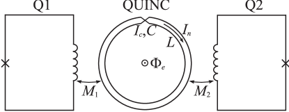
Figure 1: The QUINC with ScS quantum point contact which mediates coupling between the qubits Q1 and Q2. The loop of the coupler has inductance $L$ and the contact of the coupler has self-capacitance $C$ and critical current $I_{c}$.

It was shown in Ref. Brink, , that energy of Ising-type ZZ interaction of two flux qubits, mediated by a coupler as a nonlinear quantum element, is

$$\begin{array}[]{c}\displaystyle{J(\Phi_{e})=-\chi(\Phi_{e})M_{1}\!M_{2}I_{1}\!I_{2},\vspace{2mm}}\\ \displaystyle{\chi(\Phi_{e})\!\equiv\!\frac{1}{L_{Q}}\!=\!-\frac{dI_{n}}{d\Phi_{e}}\!=\!\frac{d^{2}E_{n}}{d\Phi_{e}^{2}}\!=\!\frac{1}{L}\!\left(\!1\!-\!\frac{d\Phi}{d\Phi_{e}}\right)\!,}\end{array}$$ (1)

where $I_{1},I_{2}$ are the superconducting currents of the basis states $\left\{\left|\uparrow\right\rangle_{i};\left|\downarrow\right\rangle_{i}\right\}$ ($i\!=\!1,2$) of the first and the second qubits; $E_{n}(\Phi_{e})$ and $I_{n}(\Phi_{e})$ are the energy of the coupler operation level and circulating in its loop superconducting current as functions of magnetic flux $\Phi_{e}$ applied to the loop, respectively; $\Phi(\Phi_{e})\!=\!\Phi_{e}\!-\!LI_{n}(\Phi)$ is the internal magnetic flux in the loop; $\chi(\Phi_{e})\!=\!E_{n}^{\prime\prime}(\Phi_{e})$ is the local curvature of the coupler operation level called the susceptibility or, equivalently, the reciprocal quantum inductance $L_{Q}^{-1}$ of the level. As seen from Eq. (1), interaction energy $J(\Phi_{e})$ between two flux qubits is determined by the susceptibility function $\chi(\Phi_{e})$, to within constant coefficients of mutual inductances and qubit currents. So we calculate the $\chi(\Phi_{e})$ function of the QUINC with ScS atomic-size contact to analyze its specific coupling properties. Note that positive values of the curvature ($\chi\!>\!0$) correspond to ferromagnetic coupling of qubits (FM, $J\!<\!0$), while negative values ($\chi\!<\!0$) to antiferromagnetic coupling (AFM, $\!J>\!0$).

It should be emphasized that a quantum inductance coupler, being a quantum element, must function in one-dimensional Hilbert space, so as not to get entangled with the qubits, thus resulting in effective four-dimensional Hilbert state space of the qubit subsystem. It can be achieved provided that (i) the operation level $E_{n}(\Phi_{e})$ is weakly-superpositional, (ii) the distances between $E_{n}$ and the neighboring levels $E_{n-1},E_{n+1}$ substantially exceed the splittings $\Delta\!E_{01}^{(1)},\Delta\!E_{01}^{(2)}$ of the qubits. Note that quantum coherent adiabatic regime of the coupler functioning allows to eliminate decohering influence of quasiparticle currents, inherent to a classical system (SQUID), on the qubit dynamics.

To analyze the QUINC with ScS atomic-size contact (such that the parameter $g\!=\!E_{J}/E_{C}\!=\!\Phi_{0}I_{c}C/(2\pi e^{2})\!\gg\!1$) at the bath temperature $T$ considerably less than any distances between adjacent energy levels of the quantum system (thus validating a zero-temperature approximation), we use the flux-representation Hamiltonian in the form Shnyrkov1 ; Leggett

$$\begin{array}[]{c}\displaystyle{\hat{H}_{C}=\frac{\hat{P}^{2}}{2M}+\hat{U}(f;f_{e})=\vspace{2mm}}\\ \displaystyle{=-\frac{\hbar^{2}}{2M}\frac{\partial^{2}}{\partial f^{2}}+\frac{\Phi_{0}I_{c}}{2\pi}\!\left[-2\left|\cos(\pi f)\right|+\frac{2\pi^{2}(f-f_{e})^{2}}{\beta_{L}}\right],}\end{array}$$ (2)

where $f=\Phi/\Phi_{0}$ and $f_{e}=\Phi_{e}/\Phi_{0}$ are the normalized internal magnetic flux $\Phi$ in the coupler loop and external magnetic flux $\Phi_{e}$ applied to the loop, $M=\Phi_{0}^{2}C$ is the respective effective mass. The quantum dynamical observable of the internal magnetic flux in the coupler loop is given by an operator $\hat{\Phi}$ conjugated to an operator $\hat{Q}$ of charge in the contact capacitance: $[\hat{\Phi},\hat{Q}]=i\hbar$ Leggett . The key feature of Hamiltonian (2) is its singular potential $U(f;f_{e})$ following from the non-sine current-phase relation of ScS quantum point contact Beenakker :

$$I_{s}(\varphi)=I_{c}\sin(\varphi/2)\,\textrm{sgn}[\cos(\varphi/2)],\,\,I_{c}=\frac{\pi\Delta_{0}}{eR_{N}}=N\frac{e\Delta_{0}}{\hbar},$$

where $\Delta_{0}$ is the superconducting energy gap, $R_{N}$ is the normal-state resistance of the contact, $N$ is an integer ($\varphi$-dependence is identical with that of the classical ScS contact Kulik ). The critical current of ScS atomic-size contact is quantized in consequence of quantization of the contact conductance $R_{N}^{-1}$ in units of $G_{0}\!=\!2e^{2}/h$, that was observed experimentally Agrait . Note that such an effective quantum Hamiltonian (2) of the superconducting loop closed by the ScS contact, with its Josephson energy ($U_{J}(\varphi)\!=\!-(I_{c}\Phi_{0}/\pi)|\cos(\varphi/2)|$) having the singular peculiarity and the dissipation vanishing at zero temperature, satisfactorily describes the experiments both (i) on macroscopic quantum tunneling phenomena in the loop with the clean ScS contact Shnyrkov3 ; Shnyrkov4 and (ii) on coherent quantum superposition of macroscopically distinct states in the three-well potential of the superconducting qutrit Shnyrkov2 . It is important to note with regard to the inner quasiparticle mechanism of dissipation in superconductors with Josephson contacts at zero temperature, that quantum fluctuations in both the ScS and SIS contacts with characteristic frequencies $\omega\ll\Delta_{0}$ were shown Khlus ; Eckern to correspond to equilibrium fluctuations of a quantum oscillator without damping and with a renormalized contact capacitance. In the opposite limit of high frequencies $\omega\gg\Delta_{0}$ the impact of quasiparticle excitations in the contacts gives rise to an effective linear dissipation described by the Caldeira-Leggett model. Due to large magnitude of the Nb gap ($\Delta_{0}/h=330\,$GHz), the quasiparticle dissipation can be neglected in the considered coupler.

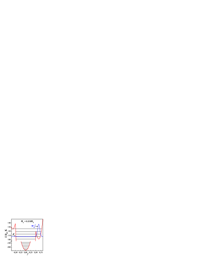
Figure 2: The coupler potential $U(f)/k_{\rm B}$ (in units of temperature) at $\beta_{L}=4.4$, $C=3.1\,$fF, $f_{e}=0.018$; $E_{n}$ is the operation level of the coupler, $|\Psi_{n}|^{2}$ is the squared wave function of the respective quantum state.

The solutions of the stationary Schrödinger equation

$$\hat{H}_{C}(f;f_{e})\,\Psi(f)=E(f_{e})\,\Psi(f)$$ (3)

with Hamiltonian (2) describe wave functions $\Psi(f)$ and energies $E(f_{e})$ of the stationary states of the coupler at a specified external magnetic flux $f_{e}$. Let us consider solutions of Eq. (3) with the following coupler parameters: $L\!=\!0.3\,$nH, $C\!=\!3.1\,$fF, $\beta_{L}\!=\!4.4$ ($I_{c}\!\approx\!4.8\,$$\mu A$) and $f_{e}\!=\!0.018$, corresponding to asymmetric three-well potential $U(f;f_{e})$, shown in Fig. 2. In this configuration, we are interested in the state with minimal energy level $E_{n}$ lying both in the right-side and the central wells of the potential. Experimentally, this state $\Psi_{n}(f)$ may be obtained from the initial ground state in the three-well symmetric potential at $\Phi_{e}\!=\!\Phi_{0}$ as a result of decreasing $\Phi_{e}$ to the required value. With decreasing $\Phi_{e}$, a central potential well transforms into a side well, where the quasiclassical state with a large quantum number ($n\!=\!25$ for $E_{n}$ in Fig. 2) is localized. The level $E_{n}$ lies far below the potential barrier top, $(U_{b}-E_{n})/k_{\rm B}\!\approx\!12.7\,$K, and separated from neighboring energy levels by a considerable interval $\Delta\!E$: $(E_{n}\!-\!E_{n-1})/k_{\rm B}\!\approx\!(E_{n+1}\!-\!E_{n})/k_{\rm B}\!\approx\!6\,$K. As the state $\Psi_{n}(f)$ is almost entirely localized in the right well, it proves to be utterly weakly-superpositional. For the parameters in Fig. 2 [such that $\chi(f_{e})\!\approx\!0$] the probability of the state $\Psi_{n}(f)$ being in the right well $P_{R}\!=\!\int_{R}\!|\Psi_{n}(f)|^{2}df\!\approx\!0.97$, and in the central well $P_{C}\!=\!\int_{C}\!|\Psi_{n}(f)|^{2}df\!\approx\!0.03$. The quantity $P_{C}$ characterizes a superpositional leakage of the state $\Psi_{n}(f)$ to the central well. Further the coupler is characterized in an operation $f_{e}$-range which is defined by a criterion of ensuring a desired fixed range of its normed susceptibility [$(LL_{Q}^{-1}\!)\!(f_{e})\!\in\!(-10\,.\,.\,10)$, see below]. When varying $f_{e}$ away from the point $f_{0}$ of zeroing of the $\chi$-function (at a given $\beta_{L}$), the $P_{C}$ magnitude increases; for curves in Fig. 3, the maximal $P_{C}\!=\!0.04$ in the operation $f_{e}$-range. With increase in $\beta_{L}$ the potential barrier between the right and the central wells grows (and so grows the depth of the right well), that causes reducing of the $P_{C}$; e.g. for $\beta_{L}=4.6$ the maximal $P_{C}\!=\!0.02$ in the operation range. At that the $P_{R}$ approaches nearer to unity.

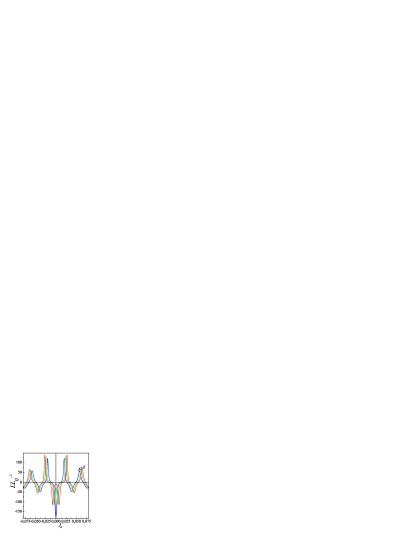
Figure 3: The function $(LL_{Q}^{-1})(f_{e})$ for $L\!=\!0.3$ nH, $\beta_{L}\!=\!4.4$, and the values of $C$: 1 – 3.0 fF, 2 – 3.05 fF, 3 – 3.10 fF.

It should be pointed out that under actual conditions the coupler state will be always to some extent decohered (being in the so-called partially-coherent state), because of finite nonzero environment temperature and influence of unavoidable decohereing (noise-originating) factors. We assume the situation in which the influence of small superpositional probability $P_{C}$ of the coupler being in the central well on its entanglement with the qubits is smoothed away due to the finite noise-induced phase dispersion of the wave function $\Psi_{n}(f)$. Thus, weak superpositionality of the coupler operation state and its large separation from the neighboring states (multiply exceeding the tunnel splittings of qubits) can make the coupler a well-defined entity not entangled with the qubits.

Because of small setting times of the operation state during variation of the external magnetic flux, estimated as $\tau\!\sim\!h/\!\Delta\!E\!\sim\!10^{-11}\,$s, the coupler will be described by the adiabatic susceptibility $\chi(\Phi_{e})$ even at rather high switching rates. Similarly to stability of the base superposition state of the qutrit toward relaxation to underlying states Shnyrkov2 , the coupler operation level will be the same stable under certain conditions. It is possible due to designing of the coupler loop in the form of a high-quality three-dimensional toroidal superconducting cavity with no resonant modes at frequencies corresponding to that of transitions from the operation level to underlying ones.

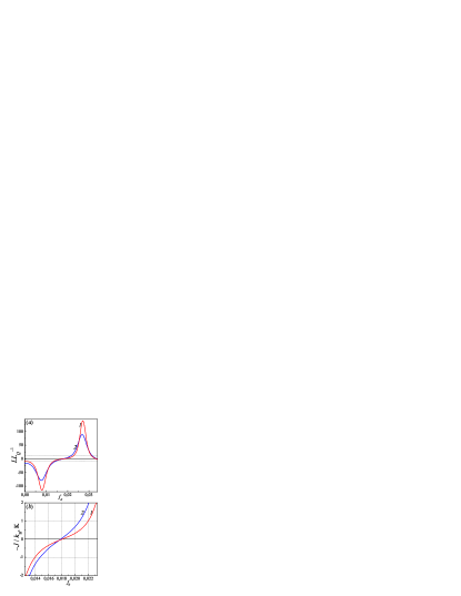
Figure 4: (a) The function $(LL_{Q}^{-1})(f_{e})$ for $L\!=\!0.3$ nH, $C\!=\!3.10$ fF and the values of $\beta_{L}$: 1 – 4.4, 2 – 4.2; (b) The function $-J(f_{e})/k_{\rm B}$ for $L\!=\!0.3$ nH, $C\!=\!3.10$ fF, $M_{1}\!=\!M_{2}\!=\!0.03\,$nH, $I_{1}\!=\!I_{2}\!=\!0.8\,\mu$A, and the values of $\beta_{L}$: 1 – 4.4, 2 – 4.2.

For practical analysis, the function $(LL_{Q}^{-1}\!)\!(f_{e})$ of the susceptibility (i.e. $L_{Q}^{-1}$) normed to the loop inductance $L$ is convenient Shnyrkov2 . It is obtained by numerical solving Eq. (3), finding $E_{n}(f_{e})$ and its double differentiation by the $f_{e}$ parameter: $(LL_{Q}^{-1}\!)\!(f_{e})\!=\!(L/\Phi_{0}^{2})d^{2}E_{n}\!/\!df_{e}^{2}$. In Fig. 3 the function $(LL_{Q}^{-1}\!)\!(f_{e})$ is shown for $\beta_{L}\!=\!4.4$ and several values of the ScS-contact capacitance. With increasing $C$, the curve $(LL_{Q}^{-1}\!)\!(f_{e})$ shifts right parallel to the x-axis. At that a form of the curve does not change qualitatively in the operation $f_{e}$-range of the coupler. In Fig. 4(a) the function $(LL_{Q}^{-1}\!)\!(f_{e})$ is shown for two different values of $\beta_{L}$. As discussed above, with increasing $\beta_{L}$ the state $\Psi_{n}(f)$ still more localizes in the right well. Nonlinearity of the $E_{n}(f_{e})$ function increases, and so the $(LL_{Q}^{-1}\!)\!(f_{e})$ rises in absolute value, with its slope at the x-axis decreased. This decrease of the susceptibility slope about the $f_{0}$ point can be compensated by widening of the coupler operation range as necessary. Fig. 4(b) shows the function $-J(f_{e})/k_{\rm B}$ (see Eq. (1)) of the mediated by the coupler inter-qubit interaction energy (in temperature units and with minus sign for convenience) for the same set of the coupler parameters as in Fig. 4(a) and the characteristic absolute values of coupler-qubit mutual inductances $M_{1}\!=\!M_{2}\!=\!0.1L$ and of the basis currents in qubits. It is seen that at chosen parameters the variation of the control external flux in the relatively small range $f_{e}\!\in\!(0.014\,.\,.\,0.022)$ ensures the wide range of variation $(-J/k_{\rm B})\!\in\!(-1\,.\,.\,1$ K) of the inter-qubit coupling energy.

III Entanglement measures

Let us now analyze properties of the two-qubit system with ZZ interaction $J(f_{e})$ mediated by the considered coupler (see Fig. 1). Having obtained eigenstates and density matrix of the system, we will explicitly find entanglement measures, widely used for characterization of the entangled states Wootters ; SM ; Bennett , and consider an example of the entanglement time variation in the studied system.

The effective Hamiltonian of the system in the tensor-product basis

$$\begin{array}[]{c}\displaystyle{\left\{\left|\uparrow\right\rangle_{1};\left|\downarrow\right\rangle_{1}\right\}\!\otimes\!\left\{\left|\uparrow\right\rangle_{2};\left|\downarrow\right\rangle_{2}\right\}=\left\{\left|\uparrow\uparrow\right\rangle;\left|\uparrow\downarrow\right\rangle;\left|\downarrow\uparrow\right\rangle;\left|\downarrow\downarrow\right\rangle\right\}}\end{array}$$ (4)

(the numbers of arrows correspond to omitted qubit indices in ”two-arrow”  states) of the four-dimensional state space, close to qubits’ degeneracy points, has the form

$$\begin{array}[]{c}\displaystyle{\hat{H}_{12}=(-\varepsilon_{1}\hat{\sigma}_{z}\!-\!\Delta_{1}\hat{\sigma}_{x})\otimes\hat{\sigma}_{0}+\hat{\sigma}_{0}\otimes(-\varepsilon_{2}\hat{\sigma}_{z}\!-\!\Delta_{2}\hat{\sigma}_{x})+\vspace{1.5mm}}\\ \displaystyle{+J(f_{e})\,\hat{\sigma}_{z}\!\otimes\hat{\sigma}_{z}=\vspace{2mm}}\\ \displaystyle{=\!\!\left(\!\begin{array}[]{cccc}-\varepsilon_{1}\!-\!\varepsilon_{2}\!+\!J&-\!\Delta_{2}&-\!\Delta_{1}&0\\ -\!\Delta_{2}&-\varepsilon_{1}\!+\!\varepsilon_{2}\!-\!J&0&-\!\Delta_{1}\\ -\!\Delta_{1}&0&\varepsilon_{1}\!-\!\varepsilon_{2}\!-\!J&-\!\Delta_{2}\\ 0&-\!\Delta_{1}&-\!\Delta_{2}&\varepsilon_{1}\!+\!\varepsilon_{2}\!+\!J\\ \end{array}\!\right)\!.}\end{array}$$ (5)

Here $\varepsilon_{1}$, $\varepsilon_{2}$ are the energy biases of first and second qubits relative to their degenerate energy levels in symmetric two-well qubit potentials, $\hat{\sigma}_{x},\hat{\sigma}_{z},\hat{\sigma}_{0}$ are the Pauli matrices. The fourth-order characteristic equation for finding eigenvalues of $\hat{H}_{12}$ [Eq.(5)]

$$\begin{array}[]{c}\displaystyle{E^{4}-2(\varepsilon_{1}^{2}\!+\!\varepsilon_{2}^{2}\!+\!\Delta_{1}^{2}\!+\!\Delta_{2}^{2}\!+\!J^{2})E^{2}-(8\varepsilon_{1}\varepsilon_{2}J)E\vspace{1mm}}\\ \displaystyle{+[\varepsilon_{1}^{4}\!+\!\varepsilon_{2}^{4}\!+\!J^{4}\!+\!(\Delta_{1}^{2}\!-\!\Delta_{2}^{2})^{2}\!+\!2J^{2}\!(\Delta_{1}^{2}\!+\!\Delta_{2}^{2})+\vspace{1mm}}\\ \displaystyle{+2(\Delta_{1}^{2}\!-\!\Delta_{2}^{2})(\varepsilon_{1}^{2}\!-\!\varepsilon_{2}^{2})\!-\!2(\varepsilon_{1}^{2}\varepsilon_{2}^{2}\!+\!\varepsilon_{1}^{2}J^{2}\!+\!\varepsilon_{2}^{2}J^{2})]=0}\end{array}$$ (6)

can be solved in radicals, e.g. by Ferrari’s method. The most interesting with relation to the quantum mechanics is the symmetric case of unbiased qubits ($\varepsilon_{1}\!=\!\varepsilon_{2}\!=\!0$) with maximal superposition and entanglement effects. In this case Eq. (6) is simplified to a biquadratic equation and the two-qubit system has the eigenenergies

$$\begin{array}[]{c}\displaystyle{E_{i}=\mp\sqrt{J^{2}+(\Delta_{1}\pm\Delta_{2})^{2}},\quad i=1,2,3,4.}\end{array}$$ (7)

We focus on the still more symmetric and indicative case of unbiased qubits with equal tunnel amplitudes ($\Delta_{1}\!=\!\Delta_{2}\!=\!\Delta\!=\!\Delta\!E_{01}/2$), in which the eigenvalues of $\hat{H}_{12}$ are

$$\begin{array}[]{c}\displaystyle{E_{1}\!=\!-\sqrt{J^{2}+4\Delta^{2}}},\,\displaystyle{E_{2}\!=\!-J},\,\displaystyle{E_{3}\!=\!J},\,\displaystyle{E_{4}\!=\!\sqrt{J^{2}+4\Delta^{2}}},\end{array}$$ (8)

and the corresponding normed eigenstates are

$$\begin{array}[]{c}\displaystyle{\left|\Psi_{1}\right\rangle=a\left|\uparrow\uparrow\right\rangle+b\left|\uparrow\downarrow\right\rangle+b\left|\downarrow\uparrow\right\rangle+a\left|\downarrow\downarrow\right\rangle},\,2(a^{2}+b^{2})\!=\!1,\vspace{1mm}\\ a\!=\!\frac{\Delta}{\sqrt{J^{2}\!+\!4\Delta^{2}}}\left(\!1+\frac{J}{\sqrt{J^{2}+4\Delta^{2}}}\right)^{\!-\frac{1}{2}}\!,\,b\!=\!\frac{1}{2}\left(\!1+\frac{J}{\sqrt{J^{2}+4\Delta^{2}}}\right)^{\!\frac{1}{2}};\vspace{3mm}\\ \displaystyle{\left|\Psi_{2}\right\rangle=\frac{1}{\sqrt{2}}\left(\left|\uparrow\downarrow\right\rangle-\left|\downarrow\uparrow\right\rangle\right);\hskip 5.69054pt\left|\Psi_{3}\right\rangle=\frac{1}{\sqrt{2}}\left(\left|\uparrow\uparrow\right\rangle-\left|\downarrow\downarrow\right\rangle\right);\vspace{3mm}}\\ \displaystyle{\left|\Psi_{4}\right\rangle=a^{\prime}\!\left|\uparrow\uparrow\right\rangle+b^{\prime}\!\left|\uparrow\downarrow\right\rangle+b^{\prime}\!\left|\downarrow\uparrow\right\rangle+a^{\prime}\!\left|\downarrow\downarrow\right\rangle},\,2(a^{\prime 2}+b^{\prime 2})\!=\!1,\vspace{1mm}\\ a^{\prime}\!=\!\frac{\Delta}{\sqrt{J^{2}\!+\!4\Delta^{2}}}\left(\!1-\frac{J}{\sqrt{J^{2}+4\Delta^{2}}}\right)^{\!-\frac{1}{2}}\!,b^{\prime}\!=\!-\frac{1}{2}\left(\!1-\frac{J}{\sqrt{J^{2}+4\Delta^{2}}}\right)^{\!\frac{1}{2}}\!.\par\end{array}$$ (9)

The density operator of the system in pure (at zero temperature) eigenstates $\left|\Psi_{i}\right\rangle$ (i=1,2,3,4) has the form

$$\begin{array}[]{c}\displaystyle{\hat{\rho}=|\Psi_{i}\rangle\langle\Psi_{i}|}\,.\end{array}$$ (10)

For definiteness sake, we focus on the ground state $|\Psi_{1}\rangle$ of the system. Taking into account Eqs. (9), we obtain the density matrix $\rho_{kl}=\langle k|\hat{\rho}|l\rangle$ (in the basis (4)) in the ground state

$$\begin{array}[]{c}\displaystyle{\rho_{kl}=\begin{pmatrix}a^{2}&ab&ab&a^{2}\\ ab&b^{2}&b^{2}&ab\\ ab&b^{2}&b^{2}&ab\\ a^{2}&ab&ab&a^{2}\\ \end{pmatrix}}\end{array}$$ (11)

(note that components of $\rho_{kl}$ are real as the initial tunneling amplitudes $\Delta_{1},\Delta_{2}$ were chosen real, without loss of generality for considering stationary states and entanglement measures). The density matrix of a pure state, such as (11), has the only nonzero eigenvalue $\lambda=1$ (as $\hat{\rho}^{2}=\hat{\rho}$ for it and thus $\lambda^{2}=\lambda$). The reduced density operators for either of the two qubits are defined as partial traces of $\hat{\rho}$ over basis vectors of the other qubit, that is

$$\begin{array}[]{c}\displaystyle{\hat{\rho}_{1}\!=\!{\rm Tr}_{(2)}\hat{\rho}=\left\langle k|\hat{\rho}|k\right\rangle\!,\,\,|k\rangle=\left|\uparrow\right\rangle_{2},\left|\downarrow\right\rangle_{2},\vspace{2mm}}\\ \displaystyle{\hat{\rho}_{2}\!=\!{\rm Tr}_{(1)}\hat{\rho}=\left\langle k|\hat{\rho}|k\right\rangle\!,\,\,|k\rangle=\left|\uparrow\right\rangle_{1},\left|\downarrow\right\rangle_{1}.}\end{array}$$ (12)

So, the reduced density matrices of the first and the second qubits in the system described by (11) are

$$\begin{array}[]{c}\displaystyle{\rho_{1}\!=\!\rho_{2}\!=\!\begin{pmatrix}1/2&2ab\vspace{1.0mm}\\ 2ab&1/2\\ \end{pmatrix}\!;\,\,\lambda_{1}\!=\!2ab+\frac{1}{2},\lambda_{2}\!=\!-2ab+\frac{1}{2},}\end{array}$$ (13)

with $\lambda_{1},\lambda_{2}$ being the eigenvalues of the equal matrices.

Now we proceed to analysis of entanglement measures. A two-qubit state

$$\begin{array}[]{c}\displaystyle{\left|\Psi\right\rangle=A\left|\uparrow\uparrow\right\rangle+B\left|\uparrow\downarrow\right\rangle+C\left|\downarrow\uparrow\right\rangle+}D\left|\downarrow\downarrow\right\rangle\end{array}$$

is entangled, that is by definition not decomposable as a tensor product of states of two qubits

$$\begin{array}[]{c}\displaystyle{(\alpha\left|\uparrow\right\rangle_{1}+\beta\left|\downarrow\right\rangle_{1})\otimes(\gamma\left|\uparrow\right\rangle_{2}+\delta\left|\downarrow\right\rangle_{2}),}\end{array}$$

if and only if the inequality $AD-BC\neq 0$ is fulfilled, which follows straight from the definition (4) of the two-qubit basis. Entanglement measure of two-qubit states

$$\begin{array}[]{c}\displaystyle{{\mathcal{E}}_{0}={\rm 4}|AD-BC|^{{\rm 2}},}\end{array}$$ (14)

is called the tangle, having such plain structure Wootters . For the ground state $\left|\Psi_{1}\right\rangle$, given by (9), we have:

$$\begin{array}[]{c}\displaystyle{{\mathcal{E}}_{0}=4(a^{2}-b^{2})^{2}=\frac{J^{2}}{J^{2}+4\Delta^{2}}=\frac{J_{0}^{2}}{1+J_{0}^{2}},}\end{array}$$ (14^′)

where $J_{0}\equiv J/(2\Delta)=J/\Delta\!E_{01}$ is the two-qubit interaction energy $J$ normed to the tunnel splitting $\Delta\!E_{01}$ of the qubits.

There is a widespread density-matrix formalism measure of entanglemet SM :

$$\begin{array}[]{c}\displaystyle{{\mathcal{E}}_{D}=\frac{4}{3}{\rm Tr}\!\left\{(\hat{\rho}-\hat{\rho}_{1}\!\otimes\!\hat{\rho}_{2})^{2}\right\}}.\end{array}$$ (15)

It quantifies the Hilbert-Schmidt distance between a density matrix and a tensor-product matrix from reduced density matrices of the two qubits. Substituting matrices (11), (13) into (15) we get for the state $\left|\Psi_{1}\right\rangle$:

$$\begin{array}[]{c}\displaystyle{{\mathcal{E}}_{D}\!=\!1\!-\!\frac{32}{3}b^{2}\!+\!\frac{128}{3}b^{4}\!-\!\frac{256}{3}b^{6}\!+\!\frac{256}{3}b^{8}\!=\!\frac{{\mathcal{E}}_{0}(2+{\mathcal{E}}_{0})}{3}.}\end{array}$$ (15^′)

The relation between ${\mathcal{E}}_{D}$ and ${\mathcal{E}}_{0}$ in (15^′) is strict for the pure states KSB .

One more popular measure is information-theoretic one called the entanglement of formation, defined as Bennett :

$$\begin{array}[]{c}\displaystyle{{\mathcal{E}}_{S}\!=\!S(\hat{\rho}_{1}\!)=\!S(\hat{\rho}_{2})\!=\!-{\rm Tr}\!\left\{\hat{\rho}_{1}{\rm log}_{2}\hat{\rho}_{1}\right\}\!=\!-\sum_{i=1}^{2}\lambda_{i}{\rm log}_{2}\lambda_{i}.}\end{array}$$ (16)

With $\lambda_{1},\lambda_{2}$ from (13), Eq.(16) gives ${\mathcal{E}}_{S}$ for the state $\left|\Psi_{1}\right\rangle$. The measure ${\mathcal{E}}_{S}$ is related to the tangle ${\mathcal{E}}_{0}$ for the pure states as well Wootters . As follows from (16), the pure states themselves have ${\mathcal{E}}_{S}\!=\!0$, seeing that their density matrices have one nonzero eigenvalue $\lambda\!=\!1$. On the other hand, the reduced density matrices of two subsystems of a system in an entangle pure state correspond to the mixed states. This property of efficient states of the subsystems is treated as their mutual ”measuring”  each other as parts of an entangled system.

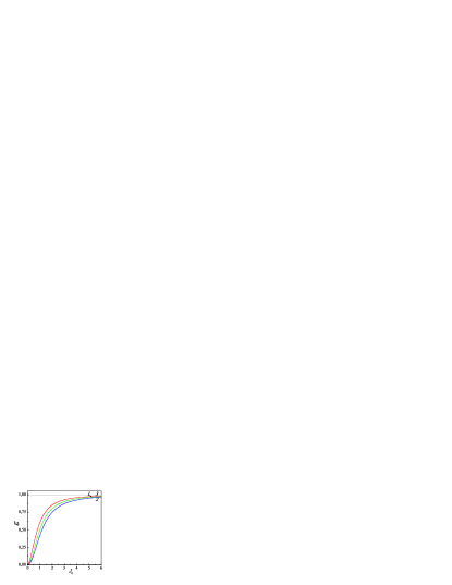
Figure 5: The entanglement measures of the two-qubit system in the ground state $\left|\Psi_{1}\right\rangle$ as functions of the dimensionless interaction parameter $J_{0}$: $\textit{1}-{\mathcal{E}}_{0}(J_{0})$, $\textit{2}-{\mathcal{E}}_{D}(J_{0})$, $\textit{3}-{\mathcal{E}}_{S}(J_{0})$.

All the entanglement measures ${\mathcal{E}}_{0},{\mathcal{E}}_{D}$ and ${\mathcal{E}}_{S}$ vanish in the tensor-product states, being positive otherwise, and maximize to unity in the most entangled states (such as states of the Bell’s basis). In Fig. 5, the ${\mathcal{E}}_{0},{\mathcal{E}}_{D},{\mathcal{E}}_{S}$ as functions of the qubits’ interaction parameter $J_{0}$, given by Eqs. (14^′), (15^′), (16), are shown for the considered two-qubit system in the ground state $\left|\Psi_{1}\right\rangle$. Due to symmetry, exactly the same expressions hold for the highest excited state $\left|\Psi_{4}\right\rangle$. At $J_{0}\!=\!0$ ($a\!=\!b\!=\!1/2$, $a^{\prime}\!=\!-b^{\prime}\!=\!1/2$), i.e. at vanishing interaction strength between the qubits, the states $|\Psi_{1}\rangle$, $|\Psi_{4}\rangle$ decompose into the product of the form

$$\begin{array}[]{c}\left|\Psi_{1}\right\rangle=\frac{1}{\sqrt{2}}(\left|\uparrow\right\rangle_{1}+\left|\downarrow\right\rangle_{1})\!\otimes\!\frac{1}{\sqrt{2}}(\left|\uparrow\right\rangle_{2}+\left|\downarrow\right\rangle_{2}),\vspace{1mm}\\ \left|\Psi_{4}\right\rangle=\frac{1}{\sqrt{2}}(\left|\uparrow\right\rangle_{1}-\left|\downarrow\right\rangle_{1})\!\otimes\!\frac{1}{\sqrt{2}}(\left|\uparrow\right\rangle_{2}-\left|\downarrow\right\rangle_{2}),\end{array}$$ (17)

so that all the entanglement measures vanish, the qubits are disentangled. Note, the reduced density matrices $\rho_{1}$ and $\rho_{2}$ in Eq.(13) describe pure states in this case (otherwise mixed ones). With increasing absolute value of $J_{0}$, all the entanglement measures steadily increase. In the characteristic point $J_{0}\!=\!1$: ${\mathcal{E}}_{0}(1)\!=\!0.5$, ${\mathcal{E}}_{D}(1)\!=\!0.4$, ${\mathcal{E}}_{S}(1)\!=\!0.6$. At $J_{0}\!\rightarrow\!\infty$, ${\mathcal{E}}_{0}=1\!-\!J_{0}^{-2}\!+\!\mbox{o}(J_{0}^{-4})$. And so, at increasing $|J|\!\gg\!\Delta$ (FM-coupling), the ground and the highest excited states tend to

$$\begin{array}[]{c}\left|\Psi_{1}\right\rangle\!\rightarrow\!\frac{1}{\sqrt{2}}(\left|\uparrow\uparrow\right\rangle\!+\!\left|\downarrow\downarrow\right\rangle),\,\,\left|\Psi_{4}\right\rangle\!\rightarrow\!\frac{1}{\sqrt{2}}(\left|\uparrow\downarrow\right\rangle\!+\!\left|\downarrow\uparrow\right\rangle),\end{array}$$ (18)

the Bell’s states having the maximal unity entanglement (while the eigenstates $\left|\Psi_{2}\right\rangle\!,\!\left|\Psi_{3}\right\rangle$, being the Bell’s states, have the unity entanglement at arbitrary $J$).

The eigenstates $\left|\Psi_{i}\right\rangle$ (9) are stationary, varying in time as $\exp(-iE_{i}t/\hbar)$ with the eigenenergies $E_{i}$ (8) (i=1,2,3,4). So the entanglement of the eigenstates is constant in time, as seen from Eq.(14) for ${\mathcal{E}}_{0}$. Let’s consider a simple dynamical model in which the two-qubit interaction under study can be turned on and off instantly. It simulates a situation, when interaction turning on/off timespan is much less than the system’s characteristic dynamical time. Suppose, the interaction $J$ is turned on between the qubits which are initially disentangled, specifically, in the product state $\left|\Psi_{1}\right\rangle$ from Eq.(17). Applying eigendecomposition of the Hamiltonian, we get the time-varying state vector

$$\begin{array}[]{c}\displaystyle{\left|\Psi\!(t)\right\rangle\!=\!e^{-i\hat{H}_{12}t/\hbar}\!\left|\Psi\!(0)\right\rangle\,,\langle k\left|\Psi\!(t)\right\rangle\!=\!(A,B,B,A),\vspace{1mm}}\\ \displaystyle{A\!=\!a(a+b)e^{-iE_{1}t/\hbar}+a^{\prime}\!(a^{\prime}+b^{\prime})e^{iE_{1}t/\hbar}},\vspace{0mm}\\ \displaystyle{B\!=\!b(a+b)e^{-iE_{1}t/\hbar}+b^{\prime}\!(a^{\prime}+b^{\prime})e^{iE_{1}t/\hbar}\,,}\end{array}$$ (19)

and the tangle

$$\begin{array}[]{c}\displaystyle{{\mathcal{E}}_{0}(t)\!=\!\frac{J_{0}^{2}}{1+J_{0}^{2}}\!\left[\!\frac{(\cos(2\pi t/t_{0}\!)-1)^{2}}{1+J_{0}^{2}}+\sin^{2}(2\pi t/t_{0}\!)\right]},\vspace{0mm}\\ \end{array}$$ (20)

where $t_{0}\!=\!h/\!(2\sqrt{J^{2}\!+\!\Delta\!E_{01}^{2}})$ is its oscillation period. At $J_{0}\!\leq\!1$, time of transition from the initial disentangled state to the maximally entangled one, with ${\mathcal{E}}_{0}^{max}\!=\![2/\!(J_{0}+J_{0}^{-1}\!)]^{2},$ is $t_{\varepsilon}\!=\!t_{0}/2$ (otherwise, $t_{\varepsilon}=(t_{0}/\!2\pi)\arccos(-J_{0}^{-2}\!)\!>\!t_{0}/4$ and ${\mathcal{E}}_{0}^{max}\!=\!1$). So, from a dynamical viewpoint, characteristic time of entangling of two initially disentangled subsystems is determined by their interaction energy $J$: $t_{\varepsilon}\!\sim\!\hbar/J$ at $J\!\sim\!\Delta$. And the mere fact of entanglement between subsystems becomes possible because of their interaction (${\mathcal{E}}_{0}(t)\!=\!0$ at $J\!=\!0$). Suppose that the interaction $J_{0}\!=\!1$ is turned off at the moment $t_{\varepsilon}$. Then the respective state vector $(0,\frac{i}{\sqrt{2}},\frac{i}{\sqrt{2}},0)$ will start to oscillate as $\langle k\left|\Psi(t)\right\rangle\!=\!(a_{f},b_{f},b_{f},a_{f})$, with $a_{f}\!=\!-\frac{\sin 2\pi t/t_{f}}{\sqrt{2}}$, $b_{f}\!=\!\frac{i\cos 2\pi t/t_{f}}{\sqrt{2}}$ and the period $t_{f}\!=\!h/\!\Delta\!E_{01}$, having constant ${\mathcal{E}}_{0}(t)\!=\!1$, that illustrates the conception of quantum nonlocality (though the latter suggesting that consistent non-paradoxical description of interaction of quantum systems requires the theoretical setting of relativistic quantum field theoryRQFT ).

IV Summary

We have analyzed the quantum inductance coupler based on a superconducting loop with ScS quantum point contact, which is intended to provide the tunable ZZ interaction between superconducting flux qubits. The following features of this coupler should be pointed out that favorably distinguish it from the analogues by principle of operation. These are (i) the relatively small operation range $\Delta f_{e}\!\sim\!0.01$ of the coupler controlling flux, ensuring the wide range of strengths $J(f_{e})$ and hence promoting reduction in operational times of the coupler; (ii) almost symmetric form of the function $J(f_{e})$ relative to the point of its vanishing in the operation range; (iii) large attainable absolute values of the inter-qubit interaction strength $|J(f_{e})/k_{\rm B}|\!\sim 1\!$ K. These features of the QUINC with ScS QPC make it optimal for coupling the superconducting niobium flux qubits with ScS QPCs as well having the tunnel splittings $\Delta\!E_{01}/k_{\rm B}\!\sim\!1\!-\!2$ K, or $\Delta\!E_{01}/h\!\sim\!20\!-\!40$ GHz Shnyrkov1 (notice that properly designed superconducting Josephson circuits with QPCs may serve as high-quality qubits, qutrits, couplers and quantum detectorsShnyrkov2 thus having great potential for the quantum information science). In such a way, having available flux qubits with the splittings $\Delta\!E_{01}/k_{\rm B}\!\simeq\!1\!$ K and couplers providing energies $|J/\!k_{\rm B}|\!\simeq\!1$ K, a multi-qubit quantum system with tunable inter-qubit coupling energies can be constructed, which will behave strongly coherently at temperatures $T\!\sim\!10^{-2}$ K, enabling implementation of quantum gates.

We showed behavior of the widely-used entanglement measures for the eigenstates of the symmetric two-qubit system with ZZ inter-qubit interaction as functions of the interaction strength $J$. With different formal definitions, all the considered measures behave qualitatively similarly in agreement with physical intuition, viz. steadily increase with increasing $J$ in the system’s ground and highest excited states. Also time variation of the entanglement (${\mathcal{E}}_{0}$-measure) in the analyzed two-qubit system was illustrated within an elementary model of piecewise-constant $J(t)$ function. With increasing $J$, the entanglement time $t_{\varepsilon}$ reduces that favors to increase the rate of computational operations in the system of coupled qubits. Simultaneously, the considered instance shows that time-controlling of the entanglement is not simple problem requiring modeling of the time dependence of inter-qubit interaction strength and realizing it experimentally to perform desired two-qubit gates.

- (1) A. Steane, Quantum Computing, Rep. Prog. Phys. 61, 117–173 (1998); arXiv:quant-ph/9708022v2.
- (2) S.Y. Kilin, Quantum information, Phys. Usp. 42, 435–452 (1999).
- (3) K.A. Valiev, Quantum computers and quantum computations, Phys. Usp. 48, 1–36 (2005).
- (4) J.L. Brylinski, R. Brylinski, Universal quantum gates, in Mathematics of Quantum Computation (Chapman and Hall/CRC Press, 1994), P. 124; arXiv:quant-ph/0108062v1.
- (5) A. Barenco, C.H. Bennett, R. Cleve, D.P. DiVincenzo, N. Margolus, P. Shor, T. Sleator, J.A. Smolin, and H. Weinfurter, Elementary gates for quantum computation, Phys. Rev. A 52, 3457 (1995).
- (6) L.H. Kauffman and S.J. Lomonaco, Braiding operators are universal quantum gates, New J. Phys. 6, 134 (2004).
- (7) D.P. DiVincenzo, The physical implementation of quantum computation, Fortschr. Phys. 48, 771 (2000).
- (8) J. Clarke, F.K. Wilhelm, Superconducting quantum bits, Nature 453, 1031 (2008).
- (9) A. Izmalkov, M. Grajcar, E. Il’ichev, Th. Wagner, H.-G. Meyer, A.Yu. Smirnov, M.H.S. Amin, A.M. van den Brink, and A.M. Zagoskin, Evidence for entangled states of two coupled flux qubits, Phys. Rev. Lett. 93, 037003 (2004).
- (10) J.B. Majer, F.G. Paauw, A.C.J. ter Haar, C.J.P.M. Harmans, and J.E. Mooij, Spectroscopy on two coupled superconducting flux qubits, Phys. Rev. Lett. 94, 090501 (2005).
- (11) B.L.T. Plourde, J. Zhang, K.B. Whaley, F.K. Wilhelm, T.L. Robertson, T. Hime, S. Linzen, P.A. Reichardt, C.-E. Wu, and John Clarke, Entangling flux qubits with a bipolar dynamic inductance, Phys. Rev. B 70, 140501(R) (2004).
- (12) A.M. van den Brink, A.J. Berkley, M. Yalowsky, Mediated tunable coupling of flux qubits, New J. Phys. 7, 230 (2005).
- (13) M.J. Storcz and F.K. Wilhelm, Design of realistic switches for coupling superconducting solid-state qubits, Appl. Phys. Lett 83, 2387 (2003).
- (14) T. Hime, P.A. Reichardt, B.L.T. Plourde, T.L. Robertson, C.-E. Wu, A.V. Ustinov, J. Clarke, Solid-state qubits with current-controlled coupling, Science 314, 1427 (2006).
- (15) R. Harris, A.J. Berkley, M.W. Johnson, P. Bunyk, S. Govorkov, M.C. Thom, S. Uchaikin, A.B. Wilson, J. Chung, E. Holtham, J.D. Biamonte, A.Yu. Smirnov, M.H.S. Amin, and A.M. van den Brink, Sign- and magnitude-tunable coupler for superconducting flux qubits, Phys. Rev. Lett. 98, 177001 (2007).
- (16) V.I. Shnyrkov, A.A. Soroka, A.M. Korolev, and O.G. Turutanov, Superposition of states in flux qubits with a Josephson junction of the ScS type, Low Temp. Phys. 38, 301 (2012).
- (17) V.I. Shnyrkov, A.A. Soroka, O.G. Turutanov, Quantum superposition of three macroscopic states and superconducting qutrit detector, Phys. Rev. B 85, 224512 (2012); arXiv:1111.6571v3 [cond-mat.supr-con].
- (18) N. Agraït, A.L. Yeyati, J.M. van Ruitenbeek, Quantum properties of atomic-sized conductors, Phys. Rep. 377, 81–279 (2003).
- (19) C.W.J. Beenakker, H. van Houten, Josephson current through a superconducting quantum point contact shorter than the coherence length, Phys. Rev. Lett. 66, 3056 (1991); C.W.J. Beenakker, H. van Houten, The superconducting quantum point contact, arXiv:cond-mat/0512610v1.
- (20) I.O. Kulik and A.N. Omelyanchouk, Josephson effect in superconducting bridges: microscopic theory, Sov. J. Low Temp. Phys. 4, 142 (1978).
- (21) A.J. Leggett, Testing the limits of quantum mechanics: motivation, state of play, prospects, J. Phys.: Condens. Matter 14, R415-R451 (2002).
- (22) I.M. Dmitrenko, V.A. Khlus, G.M. Tsoi, V.I. Shnyrkov, Quantum decay of metastable current states in RF SQUIDs, Sov. J. Low Temp. Phys. 11, 77 (1985).
- (23) I.M. Dmitrenko, V.A. Khlus, G.M. Tsoi, V.I. Shnyrkov, Macroscopic quantum tunnelling in the r.f. SQUID with S-c-S point contacts, Il Nuovo Cimento D 9, 1057 (1987).
- (24) V.A. Khlus, Quantum fluctuations in superconducting point contacts, Sov. J. Low Temp. Phys. 12, 25 (1986).
- (25) U. Eckern, G. Schön, and V. Ambegaokar, Quantum dynamics of a superconducting tunnel junction, Phys. Rev. B 30, 6419 (1984).
- (26) W.K. Wootters, Quantum entanglement as a quantifiable resource, Phil. Trans. R. Soc. Lond. A 356, 1717 (1998); W.K. Wootters, Entanglement of formation of an arbitrary state of two qubits, Phys. Rev. Lett. 80, 2245 (1998).
- (27) J. Schlienz and G. Mahler, Description of entanglement, Phys. Rev. A 52, 4396 (1995).
- (28) C.H. Bennett, H.J. Bernstein, S. Popescu, and B. Schumacher, Concentrating partial entanglement by local operations, Phys. Rev. A 53, 2046 (1996).
- (29) C. Kothe, I. Sainz, and G. Bjrk, Detecting entanglement through correlations between local observables, J. Phys: Conf. Ser. 84, 012010 (2007).
- (30) D. Buchholz and J. Yngvason, There are no causality problems for Fermi’s two-atom system, Phys. Rev. Lett. 73, 613 (1994).