Implicit embedding of prior probabilities in optimally efficient neural populations

Abstract

We examine how the prior probability distribution of a sensory variable in the environment influences the optimal allocation of neurons and spikes in a population that represents that variable. We start with a conventional response model, in which the spikes of each neuron are drawn from a Poisson distribution with a mean rate governed by an associated tuning curve. For this model, we approximate the Fisher information in terms of the density and amplitude of the tuning curves, under the assumption that tuning width varies inversely with cell density. We consider a family of objective functions based on the expected value, over the sensory prior, of a functional of the Fisher information. This family includes lower bounds on mutual information and perceptual discriminability as special cases. For all cases, we obtain a closed form expression for the optimum, in which the density and gain of the cells in the population are power law functions of the stimulus prior. Thus, the allocation of these resources is uniquely specified by the prior. Since perceptual discriminability may be expressed directly in terms of the Fisher information, it too will be a power law function of the prior. We show that these results hold for tuning curves of arbitrary shape and correlated neuronal variability. This framework thus provides direct and experimentally testable predictions regarding the relationship between sensory priors, tuning properties of neural representations, and perceptual discriminability.

1 Introduction

Many bottom up theories of neural encoding posit that sensory systems are optimized to represent signals that occur in the natural environment of an organism [1, 2]. A precise specification of the optimality of a sensory representation requires four components: (1) the family of neural transformations (that dictate how natural signals are encoded in neural activity), over which the optimum is to be taken; (2) the types of signals that are to be encoded, and their prior distribution in the natural environment; (3) the noise present in the input signals, and the additional noise that is introduced by the neural transformations; and (4) the costs (e.g., metabolic) of building, operating, and maintaining the system [3]. Although an optimal solution can be computed for some simple choices of these components (e.g., Linear response models and Gaussian signal and noise distributions [4, 5]), the general problem is intractable.

A substantial literature has considered simple population coding models in which each neuron’s mean response to a scalar variable is characterized by a tuning curve [6, 7, 8, 9, 10, 11, 12, 13, 14, e.g., ]. For these models, several papers have examined the optimization of Fisher information, which expresses a bound on the mean squared error of an unbiased estimator [15, 16, 17, 18]. In these results, the distribution of sensory variables was assumed to be uniform, and the populations were assumed to be homogeneous with regard to tuning curve shape, spacing, and amplitude.

The distribution of sensory variables encountered in the environment is often non-uniform, and it is thus of interest to understand how these variations in probability affect the design of optimal populations. It would seem natural that a neural system should devote more resources to regions of sensory space that occur with higher probability, analogous to results in coding theory [19]. At the single neuron level, several publications describe solutions in which monotonic neural response functions allocate greater dynamic range to higher probability stimuli [20, 21, 22, 23]. At the population level, non-uniform allocations of neurons with identical tuning curves have been shown to be optimal for non-uniform stimulus distributions [24, 25].

Here, we examine the influence of a sensory prior on the optimal allocation of neurons and spikes in a population, and the implications of this optimal allocation for subsequent perception. Given a prior distribution over a scalar stimulus parameter, and a resource budget of $N$ neurons with an average of $R$ spikes/sec for the entire population, we seek the optimal shapes, positions, and amplitudes of the tuning curves. We assume a population with Poisson-like spiking (which may include correlations), and consider a family of objective functions based on Fisher information. This family includes lower bounds on mutual information, and the minimum attainable perceptual discrimination performance as special cases. We then approximate the Fisher information in terms of two continuous resource variables, the density and gain of the tuning curves. This approximation allows us to obtain a closed form solution for the optimal population. For all objective functions, we find that the optimal tuning curve properties (cell density, tuning width, and gain) are power-law functions of the stimulus prior, with exponents dependent on the specific choice of objective function. Through the Fisher information, we also derive a bound on perceptual discriminability, again in the form a power-law of the stimulus prior. Thus, our framework provides direct and experimentally testable links between sensory priors, tuning properties of optimal neural representations, and perceptual discriminability. This work was initially presented in  [26, 27], and portions appear in the doctoral dissertation of the first author [28].

2 Encoding model and resource constraints

We begin with a conventional model for a population of $N$ neurons responding to a single scalar variable, $s$ [6, 7, 8, 9, 10, 11, 12, 13, 14, e.g., ]. We assume initially that the number of spikes emitted (per unit time) by the $n$th neuron is a sample from an independent Poisson process, with mean rate determined by its tuning function, $h_{n}(s)$. The probability density of the population response can be written as

$$p(\vec{r}|s)=\prod_{n=1}^{N}\frac{h_{n}(s)^{r_{n}}\ e^{-h_{n}(s)}}{r_{n}!}.$$ (1)

For now, we also assume that the tuning functions can be described by unimodal functions of arbitrary shape. We generalize this analysis to the case of monotonic (saturating) tuning curves of arbitrary shape in section 5.1. And in section 5.2, we consider more general response models that can include non-Poisson and correlated spiking.

We assume the total expected spike rate, $R$, of the population is fixed, which places a constraint on the tuning curves:

$$\int p(s)\sum_{n=1}^{N}h_{n}(s)\ \,\mathrm{d}s=R,$$ (2)

where $p(s)$ is the probability distribution of stimuli in the environment, and can have an arbitrary form. We refer to this as a sensory prior, in anticipation of its future use in Bayesian decoding of the population response.

3 Objective function

We now ask: what is the best way to represent values drawn from $p(s)$ given the limited resources of $N$ neurons and $R$ total spikes? To formulate a family of objective functions which depend on both $p(s)$, and the tuning curves, we first rely on Fisher information, $I_{f}(s)$, which is defined as [29]

$$I_{f}(s) =-\sum_{\vec{r}}p(\vec{r}|s)\ \frac{\partial^{2}}{\partial s^{2}}\log p(\vec{r}|s).$$

The Fisher information provides a measure of how accurately the population response represents the stimulus parameter, based on the encoding model. It has been used to answer theoretical questions about the influence of tuning curve shapes [15, 16, 30] and response variability [31, 32] on the representational accuracy of population codes. It has also been used in neurophysiological studies to quantify changes in coding accuracy resulting from changes in tuning curve shapes during adaptation [33, 34, 35]. For the independent Poisson noise model, the Fisher information can be expressed analytically as [6]

$$I_{f}(s)=\sum_{n=1}^{N}\frac{h_{n}^{\prime 2}(s)}{h_{n}(s)},$$

where $h^{\prime}_{n}(s)$ is the derivative of the $n^{\text{th}}$ tuning curve.

The Fisher information can also be used to express lower bounds on mutual information [24], the variance of an unbiased estimator [29], and perceptual discriminability [36]. Specifically, the mutual information, $I(\vec{r};s)$, is bounded by:

$$I(\vec{r};s)\geq H(s)-\frac{1}{2}\int p(s)\ \log\left(\frac{2\pi e}{I_{f}(s)}\right)\,\mathrm{d}s,$$ (3)

where $H(s)$ is the entropy, or amount of information inherent in $p(s)$, which is independent of the neural population. The bound is tight in the limit of low noise, which can occur as $N$ increases, $R$ increases, or both [24].

The Cramer-Rao inequality allows us to express the minimum expected squared stimulus discriminability achievable by any decoder:

$$\delta^{2}\geq\Delta^{2}\int\frac{p(s)}{I_{f}(s)}\,\mathrm{d}s.$$ (4)

The constant $\Delta$ determines the performance level at threshold in a discrimination task. The conventional Cramer-Rao bound expresses the minimum mean squared error of any estimator, and in general requires a correction for the estimator bias [29]. Here, we use it to bound the squared discriminability of the estimator, as expressed in the stimulus space. This has the advantage that it is independent of bias [36], and that it is easily (and commonly) measured in perceptual experiments.

We formulate a generalized objective function that includes the Fisher bounds on information and discriminability as special cases:

$$\mathop{\scriptstyle\arg\max}_{h_{n}(s)}\int p(s)\ f\left(\sum_{n=1}^{N}\frac{h_{n}^{\prime 2}(s)}{h_{n}(s)}\right)\,\mathrm{d}s,\qquad\quad\text{s.t.}\quad\int p(s)\sum_{n=1}^{N}h_{n}(s)\ \,\mathrm{d}s=R,$$ (5)

where $f(\cdot)$ is either the logarithm, or a power function. When $f(x)=\log(x)$, optimizing Eq. (5) is equivalent to maximizing the lower bound on mutual information given in Eq. (3). We refer to this as the infomax objective function. Otherwise, we assume $f(x)=x^{\alpha}$, for some exponent $\alpha$. Optimizing Eq. (5) with $\alpha=-1$ is equivalent to minimizing the squared discriminability bound expressed in Eq. (4). We refer to this as the discrimax objective function.

4 How to optimize?

The objective function expressed in Eq. (5) is difficult to optimize because it is non-convex. To facilitate the optimization, we first parameterize a heterogeneous neural population by warping and rescaling a homogeneous population, as specified by a cell density function, $d(s)$, and a gain function, $g(s)$. In the resulting warped population, the tuning widths are inversely proportional to the cell density. Second, we show that Fisher information can be closely approximated by a continuous function of density and gain. Finally, re-writing the objective function and constraints in these terms allows us to obtain closed-form solutions for the optimal tuning curves.

4.1 Density and gain for a homogeneous population

If $p(s)$ is uniform, then by symmetry, the Fisher information for an optimal neural population should also be uniform. We assume a convolutional population of unimodal tuning curves, evenly spaced on the unit lattice, such that they approximately “tile” the space:

$$\sum_{n=1}^{N}h(s-n)\approx 1.$$

We also assume that this population has an approximately constant Fisher information:

$$I_{f}(s) =\sum_{n=1}^{N}\frac{h^{\prime 2}(s-n)}{h(s-n)}$$

$$=\sum_{n=1}^{N}\phi(s-n)\approx I_{\rm conv}.$$ (6)

That is, we assume that the Fisher information curves for the individual neurons, $\phi(s-n)$, also tile the stimulus space. The value of the constant, $I_{\rm conv}$, is dependent on the details of the tuning curve shape, $h(s)$, which we leave unspecified. As an example, Fig. 1(a-b) shows (through numerical simulation) that the Fisher information for a convolutional population of Gaussian tuning curves, with appropriate width, is approximately constant.

Figure 1: Construction of a heterogeneous population of neurons. (a) Homogeneous population with Gaussian tuning curves on the unit lattice. The tuning width of $\sigma=0.55$ is chosen so that the curves approximately tile the stimulus space. (b) The Fisher information of the convolutional population (green) is approximately constant. (c) Inset shows $d(s)$, the tuning curve density. The cumulative integral of this density, $D(s)$, alters the positions and widths of the tuning curves in the convolutional population. (d) The warped population, with tuning curve peaks (aligned with tick marks, at locations $s_{n}=D^{-1}(n)$), is scaled by the gain function, $g(s)$ (blue). A single tuning curve is highlighted (red) to illustrate the effect of the warping and scaling operations. (e) The Fisher information of the inhomogeneous population is approximately proportional to $d^{2}(s)g(s)$.

Now we introduce two variables, a gain ($g$), and a density ($d$), that affect the convolutional population as follows:

$$h_{n}(s)=g\ h\left(d(s-\frac{n}{d})\right).$$ (7)

The gain modulates the maximum average firing rate of each neuron in the population. The density controls both the spacing and width of the tuning curves: as the density increases, the tuning curves become narrower, and are spaced closer together so as to maintain their tiling of stimulus space. The effect of these two parameters on Fisher information is:

$$I_{f}(s) =d^{2}g\sum_{n=1}^{N(d)}\phi(ds-n)$$

$$\approx d^{2}g\ I_{\rm conv}.$$

The second line follows from the assumption of Eq. (6), that the Fisher information of the convolutional population is approximately constant with respect to $s$.

The total resources, $N$ and $R$, naturally constrain $d$ and $g$, respectively. If the original (unit-spacing) convolutional population is supported on the interval $(0,Q)$ of the stimulus space, then the number of neurons in the modulated population must be $N(d)=Qd$ to cover the same interval. Under the assumption that the tuning curves tile the stimulus space, Eq. (2) implies that $R=g$ for the modulated population.

4.2 Density and gain for a heterogeneous population

Intuitively, if $p(s)$ is non-uniform, the optimal Fisher information should also be non-uniform. But note that this could potentially be achieved through inhomogeneities in either the tuning curve density or gain, and it is not obvious a priori what combination of these two functions would yield the best solution.

To solve for an optimal heterogeneous population, we generalize density and gain to be continuous functions of the stimulus, $d(s)$ and $g(s)$, that warp and scale the convolutional population:

$$h_{n}(s) =g(s_{n})\ h(D(s)-n).$$ (8)

Here, $D(s)=\int_{-\infty}^{s}d(t)dt$, the cumulative integral of $d(s)$, warps the shape of the prototype tuning curve. The value $s_{n}=D^{-1}(n)$ represents the preferred stimulus value of the (warped) $n$th tuning curve (Fig. 1(b-d)). Note that the warped population retains the tiling properties of the original convolutional population. As in the uniform case, the density controls both the spacing and width of the tuning curves. This can be seen by rewriting Eq. (8) as a first-order Taylor expansion of $D(s)$ around $s_{n}$:

$$h_{n}(s) \approx g(s_{n})\ h(d(s_{n})(s-s_{n})),$$

which is a generalization of Eq. (7).

We can now write the Fisher information of the heterogeneous population of neurons in Eq. (8) as

$$I_{f}(s) =\sum_{n=1}^{N}d^{2}(s)\ g(s_{n})\ \phi(D(s)-n)$$ (9)

$$\approx d^{2}(s)\ g(s)\ I_{\rm conv}.$$ (10)

In addition to assuming that the Fisher information is approximately constant (Eq. (6)), we have also assumed that $g(s)$ is smooth relative to the width of $\phi(D(s)-n)$ for all $n$, so that we can approximate $g(s_{n})$ as $g(s)$ and remove it from the sum. The end result is an approximation of Fisher information in terms of the continuous parameterization of cell density and gain. As earlier, the constant $I_{\rm conv}$ is determined by the precise shape of the tuning curves.

As in the homogeneous case, the global resource values $N$ and $R$ will place constraints on $d(s)$ and $g(s)$, respectively. In particular, we require that $D(\cdot)$ map the entire input space onto the range $[1,N]$. Thus, for an input space covering the real line, we require $D(-\infty)=1$ and $D(\infty)=N$ (or equivalently, $\int d(s)\,\mathrm{d}s=N$). To attain the proper rate, we use the fact that the warped tuning curves sum to unity (before multiplication by the gain function), along with Eq. (2), to obtain the constraint $\int p(s)g(s)\,\mathrm{d}s=R$.

4.3 Objective function and solution for a heterogeneous population

Approximating Fisher information as proportional to squared density and gain allows us to re-write the objective function and resource constraints of Eq. (5) as

$$\mathop{\scriptstyle\arg\max}_{d(s),g(s)}\int p(s)\ f\left(d^{2}(s)\ g(s)\right)\,\mathrm{d}s,\quad\quad\text{s.t.}\quad\int d(s)\,\mathrm{d}s=N,\quad\text{and}\quad\int p(s)g(s)\,\mathrm{d}s=R.$$ (11)

A closed-form optimum of this objective function is easily determined using calculus of variations. Specifically, one can compute the gradient of the Lagrangian, set to zero, and solve the resulting system of equations (see Appendix A). Solutions are provided in Table 1 for the infomax, discrimax, and the general power cases.

	Infomax	Discrimax	General
Optimized function:	$f(x)=\log x$	$f(x)=-x^{-1}$	$f(x)=-x^{\alpha}$, $\alpha<\frac{1}{3}$
Density (Tuning width)-1 $d(s)$	$Np(s)$	$\propto Np^{\frac{1}{2}}(s)$	$\propto Np^{\frac{\alpha-1}{3\alpha-1}}(s)$
Gain $g(s)$	$R$	$\propto Rp^{-\frac{1}{2}}(s)$	$\propto Rp^{\frac{2\alpha}{1-3\alpha}}(s)$
Fisher information $I_{f}(s)$	$\propto RN^{2}p^{2}(s)$	$\propto RN^{2}p^{\frac{1}{2}}(s)$	$\propto RN^{2}p^{\frac{2}{1-3\alpha}}(s)$
Discriminability bound    $\delta_{\rm min}(s)$	$\propto p^{-1}(s)$	$\propto p^{-\frac{1}{4}}(s)$	$\propto p^{\frac{1}{3\alpha-1}}(s)$

Table 1: Optimal heterogeneous population properties, for objective functions specified by Eq. (11).

In all cases, the solution specifies a power-law relationship between the prior, and the density and gain of the tuning curves. In general, all solutions allocate more neurons, with correspondingly narrower tuning curves, to higher-probability stimuli. In particular, the infomax solution corresponds to a population with constant gain, and allocates an approximately equal amount of probability mass to each neuron, as one might intuitively expect from coding theory (Fig. 2(a-b)). The shape of the optimal gain function depends on the objective function: for $\alpha<0$, neurons with lower firing rates are used to represent stimuli with higher probabilities, and for $\alpha>0$, neurons with higher firing rates are used for stimuli with higher probabilities. Note also that the global resource values, $N$ and $R$, enter only as scale factors on the overall solution. As a result, if one or both of these factors are unknown, the solution still provides a unique specification of the shapes of $d(s)$ and $g(s)$, which can be tested against experimental data (Fig. 2(c-e)).

In addition to power-law relationships between tuning properties and sensory priors, our formulation offers a direct relationship between the sensory prior and perceptual discriminability. This can be obtained by substituting the optimal solutions for $d(s)$ and $g(s)$ into Eq. (9), and using the resulting Fisher information to bound the discriminability, $\delta(s)\geq\delta_{\rm min}(s)\equiv\Delta/\sqrt{I_{f}(s)}$ [36]. The resulting expressions are provided in Table 1. In general, the solutions predict that discrimination thresholds should be lower for more frequently occurring stimuli. In particular, the infomax solution predicts that inverse thresholds (discriminability) should be directly proportional to the prior (Fig. 2(f)).

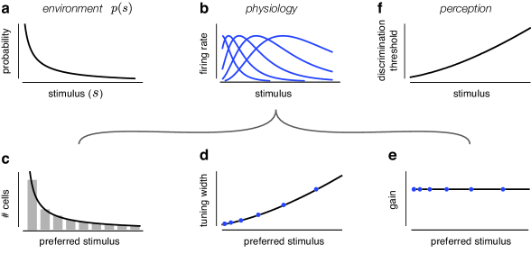
Figure 2: Infomax predictions of the relationship between environment, physiology, and perceptual discriminability. (a) An example of a probability distribution over a sensory attribute, $s$, which can be directly measured from the environment. (b) Tuning curves of a neural population designed to maximize the amount of information transmitted about stimuli drawn from the prior distribution in Panel a. (c-e) Experimentally accessible attributes of the infomax population in Panel b, and their corresponding predictions in terms of the prior distribution (black), as expressed in Table 1. (c) A histogram of the preferred stimuli (stimuli associated with the peaks of the tuning curves) of the neurons is an estimate of local cell density, which should be proportional to the prior distribution. (d) The tuning widths of the neurons (measured as the full width at half maximum of the tuning curves) should be inversely proportional to the prior distribution. (e) The gain, measured as the maximum average firing rate of each of the neurons, should be constant. (f) Minimum achievable discrimination thresholds of a perceptual system operating on the responses of an infomax population should be inversely proportional to the prior distribution.

5 Extensions

5.1 Monotonic tuning curves

Thus far we have solved for the optimal cell density and gain for warping and scaling a homogeneous population of unimodal tuning curves. However, many neurons exhibit monotonic tuning to intensity variables such as contrast, or sound pressure level. The influence of continuous cell density and gain on the Fisher information of a homogeneous population of monotonic tuning curves is the same as in the unimodal case (Eq. (10)), again assuming that the Fisher information curves of the homogeneous population tile. The constraint on $N$ is also same. However, the total spiking cost fundamentally differs. Neurons with monotonic tuning curves saturate, and thus the entire population will be active at the high range of stimulus values, which incurs a large metabolic cost for encoding these values. Intuitively, this metabolic penalty can be reduced by lowering the gains of neurons tuned to the low end of the stimulus range, or by adjusting the cell density such that there are more tuning curves tuned to the high end of the stimulus range. It is not obvious how the reductions in metabolic cost for these coding strategies should trade off with the optimal coding of sensory information.

To derive the optimal monotonic coding scheme, we first parameterize a heterogeneous population of monotonic tuning curves by warping and scaling the derivatives of a homogeneous population of monotonic tuning curves:

$$h_{n}(s)=\int_{-\infty}^{s}h_{n}^{\prime}(t)\,\mathrm{d}t=\int_{-\infty}^{s}g(s_{n})d(t)h^{\prime}(D(t)-n)\,\mathrm{d}t.$$ (12)

This expression is similar to the parameterization of a heterogeneous population of unimodal tuning curves (Eq. (8)), except here, $h(\cdot)$ is now a prototype monotonic tuning curve. The density controls both the number of tuning curves and their slopes, which are inversely proportional to the cell density. The derivatives of the (warped) monotonic tuning curves, $h^{\prime}(D(t)-n)$, will be unimodal functions, allowing us to use similar approximations and intuitions developed for the unimodal case. In particular, we assume that the derivatives of the tuning curves tile such that $\sum_{n=1}^{N}h^{\prime}(D(t)-n)\approx 1$.

The total spike count can be expressed from Eqs. (2 & 12) as,

$$R =\int_{-\infty}^{\infty}p(s)\int_{-\infty}^{s}d(t)\sum_{n=1}^{N}g(s_{n})h^{\prime}(D(t)-n)\,\mathrm{d}t\,\mathrm{d}s.$$

We define a continuous version of the gain as $g(t)=\sum_{n=1}^{N}g(s_{n})h^{\prime}(D(t)-n)$ which allows us to approximate the total number of spikes as

$$R =\int_{-\infty}^{\infty}p(s)\int_{-\infty}^{s}d(t)g(t)$$

$$=\int_{-\infty}^{\infty}\left(1-P(s)\right)d(s)g(s)\,\mathrm{d}s$$

In the second step, we performed integration by parts and defined $P(s)=\int_{-\infty}^{s}p(t)\,\mathrm{d}t$ as the cumulative density function of the sensory prior. The constraint on the total number of spikes is very different than the bell-shaped tuning curve case, as it now depends on the cell density and the cumulative distribution of the sensory prior, and will thus affect the optimal solutions for cell density and gain.

We reformulate the original optimization problem of Eq. (5) for monotonic tuning curves as:

$$\mathop{\scriptstyle\arg\max}_{d(s),g(s)}\int p(s)\ f\left(d^{2}(s)\ g(s)\right)\,\mathrm{d}s,\quad\quad \text{s.t.}\quad\hskip 5.0pt\int d(s)\,\mathrm{d}s=N,$$ (13)

$$\text{and}\quad\int\left(1-P(s)\right)d(s)g(s)\,\mathrm{d}s=R.$$

A closed-form optimum of this objective function is easily determined by taking the gradient of the Lagrangian, setting to zero, and solving the resulting system of equations. Solutions are provided in Table. 2 for the infomax, discrimax, and general power cases, in addition to solutions for the optimal Fisher information and minimum achievable discrimination thresholds achievable by a subsequent perceptual system.

	Infomax	Discrimax	General
Optimized:	$f(x)=\log x$	$f(x)=-x^{-1}$	$f(x)=-x^{\alpha}$, $\alpha<\frac{1}{3}$
Density $d(s)$	$Np(s)$	$\propto Np(s)^{\frac{1}{3}}\left[1-P(s)\right]^{\frac{1}{3}}$	$\propto Np(s)^{\frac{1}{1-2\alpha}}\left[1-P(s)\right]^{\frac{\alpha}{2\alpha-1}}$
Gain $g(s)$	$RN^{-1}\left[1-P(s)\right]^{-1}$	$RN^{-1}\left[1-P(s)\right]^{-1}$	$RN^{-1}\left[1-P(s)\right]^{-1}$
Fisher. $I_{f}(s)$	$\propto RNp^{2}(s)\left[1-P(s)\right]^{-1}$	$\propto RNp^{\frac{2}{3}}(s)\left[1-P(s)\right]^{-\frac{1}{3}}$	$\propto RNp^{\frac{2}{1-2\alpha}}(s)\left[1-P(s)\right]^{\frac{1}{2\alpha-1}}$
Discrim.    $\delta_{\rm min}(s)$	$\propto p^{-1}(s)\left[1-P(s)\right]^{\frac{1}{2}}$	$\propto p^{-\frac{1}{3}}(s)\left[1-P(s)\right]^{\frac{1}{6}}$	$\propto p^{\frac{1}{2\alpha-1}}(s)\left[1-P(s)\right]^{\frac{1}{2-4\alpha}}$

Table 2: Optimal heterogeneous population properties, for objective functions specified by Eq. (13).

For all objective functions, the solutions for the optimal density, gain, and discriminability are products of power law functions of the sensory prior, and its cumulative distribution. In general, all solutions allocate more neurons with greater dynamic range to more frequently occurring stimuli. Unlike the solutions for unimodal tuning curves (Table 1), the optimal gain is the same for all objective functions: for a neuron tuned to a particular stimulus value, the optimal gain is inversely proportional to the probability of all stimuli occurring after that stimulus value. Intuitively, this solution allocates lower gains to neurons tuned to the low end of the stimulus range, which is metabolically less costly. The global resource values $N$ and $R$ again only appear as scale factors in the overall solution, allowing us to easily compare the predicted relationships to experimental data, even when $N$ and $R$ are not known.

5.2 Generalization to Poisson-like noise distributions

Our results depend on the assumption that neuronal variability is Poisson distributed and neural responses are statistically independent. In a Poisson model, the variance of the neural responses is directly proportional to the mean responses, which has been observed experimentally in some cases [37], but may not be true in general. In addition, the assumption that neuronal responses are statistically independent conditioned on the stimulus value is often violated [38, 39].

Here, we generalize the results to a family of “Poisson-like” response models [14, 40], that allow for stimulus dependent correlations and an arbitrary linear relationship between mean and variance of the population response. We assume the probability density of the population response can be written as

$$p(\vec{r}|s) =f(\vec{r})\exp\left[\boldsymbol{\eta}(s)^{T}\vec{r}-A(\boldsymbol{\eta})\right].$$ (14)

This distribution belongs to the exponential family with linear sufficient statistics where the parameter $\boldsymbol{\eta}(s)$ is a matrix of the natural parameters of the distribution with the $n^{\text{th}}$ column equal to $\eta_{n}(s)$, $A(\boldsymbol{\eta})$ is a (log) normalizing constant that ensures the distribution integrates to one, and $f(\vec{r})$ is an arbitrary function of the firing rates. The independent Poisson noise model considered in Eq. (1) is a member of this family of distributions with parameters: $\boldsymbol{\eta}(s)=\log{\bf h(s)}$ where ${\bf h(s)}$ is a matrix of tuning curves with the $n^{\text{}th}$ column given $h_{n}(s)$, $A(\boldsymbol{\eta})=\sum_{n=1}^{N}\exp(\eta_{n})$, and $f(\vec{r})=\prod_{n=1}^{N}\frac{1}{r_{n}!}$.

All of our objective functions depend on an analytical form for the Fisher information in terms of tuning curves, which is then expressed in terms of density and gain. To derive the Fisher information for the response model in Eq. (14), we start by noting that the derivative of natural parameters is related to the stimulus dependent covariance matrix of the population responses, $\Sigma(s)$, and the derivative of the tuning curves as [14, 40],

$$\frac{\partial\boldsymbol{\eta}}{\partial s}=\Sigma^{-1}(s)\frac{\partial{\bf h}}{\partial s}.$$ (15)

The term $\Sigma^{-1}(s)$ is the inverse of the covariance matrix, and is often referred to as a precision matrix.

The Fisher information matrix about the natural parameters is simply equal to the covariance matrix [29],

$$I_{f}\left[\boldsymbol{\eta}(s)\right]=\Sigma(s).$$ (16)

The local Fisher information about the stimulus, $s$, can be derived from the chain rule as,

$$I_{f}(s) =\frac{\partial\boldsymbol{\eta}}{\partial s}^{T}I_{f}\left[\boldsymbol{\eta}(s)\right]\frac{\partial\boldsymbol{\eta}}{\partial s}.$$

After substituting the relationships in Eq. (15 & 16) into this expression we obtain the final expression for the local Fisher information

$$I_{f}(s) =\frac{\partial{\bf h}}{\partial s}^{T}\Sigma^{-1}(s)\frac{\partial{\bf h}}{\partial s}.$$ (17)

The influence of Fisher information on coding accuracy is now directly dependent on knowledge of stimulus dependent (inverse) covariance matrix. Estimating such a precision matrix from experimental data is technically challenging (although see [39]). Here, we assume a biologically plausible precision matrix that allows for neuronal variability to be proportional to the mean firing rate, and the responses of nearby neurons to be correlated [31]. For a homogeneous neural population, $h_{n}(s)=h(s-n)$, we express each element in the precision matrix as,

$$\Sigma_{n,m}^{-1}(s)=\frac{\alpha\delta_{n,m}+\beta(\delta_{n,m+1}+\delta_{n+1,m})}{\sqrt{h(s-n)h(s-m)}}.$$ (18)

The parameter $\alpha$ controls a linear relationship between the mean response and the variance of the response for all the neurons. The parameter $\beta$ controls the degree of the correlations, and $\delta_{n,n}=1$ for all $n$ while $\delta_{n,m}=0$ if $n\neq m$. The Fisher information of a homogeneous population may now be expressed from Eqs. (17 &18) as,

$$I_{f}(s) =\alpha\sum_{n=1}^{N}\phi(s-n)\hskip 6.0pt+\beta\sum_{n,m=n\pm 1}\frac{h^{\prime}(s-n)h^{\prime}(s-m)}{\sqrt{h(s-n)h(s-m)}}$$

$$\approx\alpha I_{\text{conv}}+\beta I_{\text{corr}}$$

In the last step we make two assumptions. First, we assume (as for the independent Poisson case) the Fisher information curves, $\phi(s-n)$, of the homogeneous population tile such that they sum to the constant, $I_{\text{conv}}$. Second, we assume that the cross terms, $\frac{h^{\prime}(s-n)h^{\prime}(s-m)}{\sqrt{h(s-n)h(s-m)}}$, also tile such that they sum to the constant, $I_{\text{corr}}$.

The Fisher information for a heterogeneous population, obtained by warping and scaling the homogeneous population by the density and gain is

$$I_{f}(s) =d^{2}(s)\alpha\sum_{n=1}^{N}g(s_{n})\phi(D(s)-n)$$ (19)

$$\hskip 12.0pt+d^{2}(s)\beta\sum_{n,m=n\pm 1}\frac{g(s_{n})g(s_{m})}{\sqrt{g(s_{n})g(s_{m})}}\frac{h^{\prime}(D(s)-n)h^{\prime}(D(s)-m)}{\sqrt{h(D(s)-n)h(D(s)-m)}}$$

$$\approx d^{2}(s)g(s)\left[\alpha I_{\text{conv}}+\beta I_{\text{corr}}\right].$$ (20)

In the second step we make three assumptions. First, (as for the independent Poisson case) we assume $g(s)$ is smooth relative to the width of $\phi(D(s)-n)$ for all $n$, so that we can approximate $g(s_{n})$ as $g(s)$. Second, we assume that the neurons are sufficiently dense such that $\frac{g(s_{n})g(s_{m})}{\sqrt{g(s_{n})g(s_{m})}}\approx g(s_{n})$. Finally, we assume $g(s)$ is also smooth relative to the width of the cross terms. As a result, the gain factors can be approximated by same the continuous gain function, $g(s)$, and can be pulled out of both sums.

Given the form of the Fisher information (Eq. (20)), we conclude that the optimal solutions for the density and gain are the same as those expressed in Tables 2 & 1, which were derived for an independent Poisson noise model ($\alpha=1,\beta=0$). The values of the Fisher information, and minimum achievable discrimination thresholds now depend on three additional scale factors, $\alpha$, $\beta$, and $I_{\text{corr}}$, that characterize the correlated variability of the population code.

6 Discussion

We have examined the influence of sensory priors on the optimal allocation of neural resources, as well as the implications of this optimal allocation on subsequent perception. For a family of objective functions, we obtain closed-form solutions specifying power law relationships between the prior probability distribution of a variable in the environment, the tuning properties of a population that encodes that variable, and the minimum perceptual discrimination thresholds achievable for that variable. The predictions are easily testable, and preliminary evidence indicates that the infomax solution is consistent with physiological and perceptual data for several sensory attributes [27, 28].

Our analysis requires several approximations and assumptions in order to arrive at an analytical solution. First, we rely on lower bounds on mutual information and discriminability, each based on Fisher information. Fisher information is known to provide a poor bound on mutual information when there are a small number of neurons, a short decoding time, or non-smooth tuning curves [24, 41]. It also provides a poor bound on supra-threshold discriminability [30, 42]. It is worth noting, however, we do not require the bounds on either information or discriminability to be tight, but rather that their optima be close to that of their corresponding true objective functions. In addition, our preliminary evidence indicates that, at least for typical experimental settings, both physiological and perceptual data appear to be consistent with the infomax version of our theory [27, 28]. We also made several assumptions in deriving our results: (1) the tuning curves, $h(D(s)-n)$, or in the monotonic case their derivatives, $h^{\prime}(D(s)-n)$, evenly tile the stimulus space; (2) the single neuron Fisher informations, $\phi(D(s)-n)$, evenly tile the stimulus space; and (3) the gain function, $g(s)$, varies slowly and smoothly over the width of $\phi(D(s)-n)$. These assumptions allow us to approximate Fisher information in terms of cell density and gain (Fig.  1(e)), to express the resource constraints in simple form, and to obtain a closed-form solution to the optimization problem.

Our framework offers an important generalization of the population coding literature, allowing for non-uniformity of sensory priors, and corresponding heterogeneity in tuning and gain properties. Nevertheless, it suffers from the main simplification found throughout that literature: the tuning curve response model is restricted to a single (one-dimensional) stimulus attribute. Real sensory neurons exhibit selectivity for multiple attributes. If the environmental distribution (prior) for those attributes is separable (i.e., if the values of those attributes are statistically independent) then an efficient code can be constructed separably. That is, each neuron could have joint tuning arising from the product of a tuning curve for each attribute. But extending the theory to handled multiple attributes with statistical dependencies is not straightforward.

Our formulation assumes the sensory attribute of interest is drawn from a fixed and stable distribution. However, the distribution of sensory inputs can vary according to context, and it is of interest to consider how the theory might be generalized to adjust to such changes. A potential clue comes from the physiology: a large body of literature describes adaptive changes in neural gain at time scales ranging from milliseconds to hours. These have been interpreted as homeostatic mechanisms whose purpose is to maintain a high level of information transmission [43, 44, 45]. How does this fit with our predictions? A potential interpretation is that tuning curves, which presumably arise from the strength of synaptic connections, are established and adjusted over slow time scales, so as to efficiently capture the heterogeneities in stable environmental distributions, whereas the gains of individual neurons are adjusted more rapidly, so as to adapt to fluctuating heterogeneities in input intensity, local metabolic resources, or task-related requirements.

Finally, the structure of our optimal population has direct implications for Bayesian decoding, a problem that has received much attention in recent literature [46, 14, 13, 47, 48, e.g., ]. A Bayesian decoder must have knowledge of prior probabilities, but an often-overlooked issue is how such knowledge is obtained and represented in the brain [47]. Our efficient coding solution provides a mechanism whereby the prior is implicitly encoded in the arrangement and gains of tuning curves. Recent publications [49, 50, 51, 52] have proposed that a population-vector computation (i.e., the average of the preferred stimuli of the neurons, weighted by their corresponding responses), coupled with an inhomogeneous arrangement of tuning curves, could provide a simple means for the brain to approximate a Bayesian estimate. For the case of an infomax population, we have derived a decoder that more closely approximates a Bayesian least-squares estimator. Similar to the population vector, it computes a weighted average of the preferred stimuli, but the weights are constructed by linearly combining and then exponentiating the responses [53, 28]. Thus, efficient population representations may offer unforeseen benefits for explaining subsequent stages of sensory processing.

Appendix A Solution for the infomax objective function with bell-shaped tuning curves

The optimum of the objective function in Eq. (11) is easily determined using the method of Lagrange multipliers. As an example, consider the case when $f(\cdot)=\log(\cdot)$, which corresponds to optimization of the Fisher bound on mutual information between the input signal and the population response. The Lagrangian for this case is expressed as:

$$L(d(s),g(s),\lambda_{1},\lambda_{2})=\int p(s)\log{\left(d^{2}(s)g(s)\right)}\,\mathrm{d}s+\lambda_{1}\left(\int d(s)\,\mathrm{d}s-N\right)+\lambda_{2}\left(\int p(s)g(s)\,\mathrm{d}s-R\right).$$

The optimal cell density and gain that satisfy the resource constraints are determined by setting the variational gradient of the Lagrangian to zero, and solving the resulting system of equations:

$$\frac{\partial L}{\partial d(s)} =2p(s)d^{-1}(s)+\lambda_{1}=0$$ (21)

$$\frac{\partial L}{\partial g(s)} =p(s)g^{-1}(s)+\lambda_{2}p(s)=0$$ (22)

$$\frac{\partial L}{\partial\lambda_{1}} =\int d(s)\,\mathrm{d}s-N=0$$ (23)

$$\frac{\partial L}{\partial\lambda_{2}} =\int p(s)g(s)-R=0.$$ (24)

The optimal cell density and gain are determined from Eqs. (21 & 22) as:

$$d(s) =-2\lambda_{1}^{-1}p(s)$$ (25)

$$g(s) =-1\lambda_{2}^{-1}$$ (26)

The unknown Lagrange multipliers can be determined by substituting these expressions into Eqs. (23 & 24) and solving. The result is:

$$\lambda_{1} =-2N^{-1}$$

$$\lambda_{2} =-R^{-1}$$

Substituting these expressions into Eqs. (25 & 26) yields the Infomax solution expressed in Table 1. The same method was used to derive the rest of the solutions expressed in Tables 1 & 2.

References

- [1] F Attneave. Some informational aspects of visual perception. Psychological Review, 61(3):183–193, 1954.
- [2] H Barlow. Possible principles underlying the transformation of sensory messages. Sensory Communication, pages 217–234, 1961.
- [3] EP Simoncelli and BA Olshausen. Natural image statistics and neural representation. Annual Review of Neuroscience, 24(1):1193–1216, 2001.
- [4] JJ Atick and AN Redlich. Towards a theory of early visual processing. Neural Computation, 2(3):308–320, 1990.
- [5] E. Doi, J. Gauthier, G. Field, J. Shlens, A. Sher, M. Greschner, T. Machado, L. Jepson, K. Mathieson, D. Gunning, A. Litke, L. Paninski, E. J. Chichilnisky, and E. P. Simoncelli. Efficient coding of spatial information in the primate retina. J. Neuroscience, 2012. To appear.
- [6] HS Seung and H Sompolinsky. Simple models for reading neuronal population codes. Proceedings of the National Academy of Sciences, 90(22):10749–10753, November 1993.
- [7] E Salinas and LF Abbott. Vector reconstruction from firing rates. Journal of Computational Neuroscience, 1(1-2):89–107, June 1994.
- [8] HP Snippe. Parameter extraction from population codes: A critical assessment. Neural Computation, 8(3):511–529, 1996.
- [9] TD Sanger. Probability density estimation for the interpretation of neural population codes. J Neurophysiol, 76(4):2790–2793, October 1996.
- [10] K Zhang, I Ginzburg, BL McNaughton, and TJ Sejnowski. Interpreting neuronal population activity by reconstruction: Unified framework with application to hippocampal place cells. Journal of Neurophysiology, 79(2):1017–1044, February 1998.
- [11] RS Zemel, P Dayan, and A Pouget. Probabilistic interpretation of population codes. Neural Computation, 10(2):403–430, February 1998.
- [12] A Pouget, P Dayan, and RS Zemel. Inference and computation with population codes. Annu Rev Neurosci, 26:381–410, 2003.
- [13] M Jazayeri and JA Movshon. Optimal representation of sensory information by neural populations. Nature Neuroscience, 9(5):690–696, 2006.
- [14] WJ Ma, JM Beck, PE Latham, and A Pouget. Bayesian inference with probabilistic population codes. Nature Neuroscience, 9(11):1432–1438, October 2006.
- [15] K Zhang and TJ Sejnowski. Neuronal tuning: To sharpen or broaden? Neural Computation, 11(1):75–84, January 1999.
- [16] A Pouget, S Deneve, JC Ducom, and PE Latham. Narrow versus wide tuning curves: What’s best for a population code? Neural Computation, 11(1):85–90, January 1999.
- [17] WM Brown and A Bäcker. Optimal neuronal tuning for finite stimulus spaces. Neural Computation, 18(7):1511–1526, July 2006.
- [18] MA Montemurro and S Panzeri. Optimal tuning widths in population coding of periodic variables. Neural Computation, 18(7):1555–1576, July 2006.
- [19] A Gersho and RM Gray. Vector quantization and signal compression. Kluwer Academic Publishers, Norwell, MA, 1991.
- [20] SB Laughlin. A simple coding procedure enhances a neuron’s information capacity. Zeitschrift Für Naturforschung., 36(9-10):910–912, 1981.
- [21] JP Nadal and N Parga. Non linear neurons in the low noise limit: A factorial code maximizes information transfer. Network: Computation in Neural Systems, 1994.
- [22] T von der Twer and DI MacLeod. Optimal nonlinear codes for the perception of natural colours. Network, 12(3):395–407, August 2001.
- [23] MD McDonnell and NG Stocks. Maximally informative stimuli and tuning curves for sigmoidal rate-coding neurons and populations. Physical Review Letters, 101(5):58103, 2008.
- [24] N Brunel and JP Nadal. Mutual information, fisher information, and population coding. Neural Computation, 10(7):1731–1757, September 1998.
- [25] NS Harper and D McAlpine. Optimal neural population coding of an auditory spatial cue. Nature, 430(7000):682–686, August 2004.
- [26] D. Ganguli and E. P. Simoncelli. Representation of environmental statistics by neural populations. In Computational and Systems Neuroscience (CoSyNe), Salt Lake City, Utah, February 2010.
- [27] D Ganguli and EP Simoncelli. Implicit encoding of prior probabilities in optimal neural populations. In J Lafferty, CKI Williams, J Shawe-Taylor, RS Zemel, and A Culotta, editors, Advances in Neural Information Processing Systems (NIPS), volume 23, pages 658–666, Salt Lake City, Utah, 2010.
- [28] Deep Ganguli. Efficient coding and Bayesian inference with neural populations. PhD thesis, Center for Neural Science, New York University, New York, NY, September 2012.
- [29] D Cox and D Hinkley. Theoretical statistics. London: Chapman and Hall., 1974.
- [30] M Shamir and H Sompolinsky. Implications of neuronal diversity on population coding. Neural Computation, 18(8):1951–1986, 2006.
- [31] LF Abbott and P Dayan. The effect of correlated variability on the accuracy of a population code. Neural Computation, 11(1):91–101, January 1999.
- [32] P Seriès, PE Latham, and A Pouget. Tuning curve sharpening for orientation selectivity: coding efficiency and the impact of correlations. Nature neuroscience, 7(10):1129–1135, October 2004.
- [33] I Dean, NS Harper, and D McAlpine. Neural population coding of sound level adapts to stimulus statistics. Nature Neuroscience, 8(12):1684–1689, 2005.
- [34] S Durant, CWG Clifford, NA Crowder, NSC Price, and MR Ibbotson. Characterizing contrast adaptation in a population of cat primary visual cortical neurons using fisher information. Journal of the Optical Society of America, 24(6):1529–1537, June 2007.
- [35] DA Gutnisky and V Dragoi. Adaptive coding of visual information in neural populations. Nature, 452(7184):220–224, March 2008.
- [36] P Seriès, AA Stocker, and Simoncelli EP. Is the homunculus “aware” of sensory adaptation? Neural Computation, 21(12):3271–3304, September 2009.
- [37] KH Britten, MN Shadlen, WT Newsome, and JA Movshon. Responses of neurons in macaque MT to stochastic motion signals. Visual neuroscience, 10(6):1157–1169, December 1993.
- [38] E Zohary, MN Shadlen, and WT Newsome. Correlated neuronal discharge rate and its implications for psychophysical performance. Nature, 370(6485):140–143, July 1994. PMID: 8022482.
- [39] A Kohn and MA Smith. Stimulus dependence of neuronal correlation in primary visual cortex of the macaque. The Journal of Neuroscience, 25(14):3661–3673, April 2005.
- [40] JM Beck, WJ Ma, PE Latham, and A Pouget. Probabilistic population codes and the exponential family of distributions. Prog Brain Res, 165:509–519, 2007.
- [41] M Bethge, D Rotermund, and K Pawelzik. Optimal short-term population coding: When fisher information fails. Neural Computation, 14(10):2317–2351, October 2002.
- [42] P Berens, S Gerwinn, A Ecker, and M Bethge. Neurometric function analysis of population codes. In Advances in Neural Information Processing Systems 22, page 90–98, 2009.
- [43] MJ Wainwright. Visual adaptation as optimal information transmission. Vision research, 39(23):3960–3974, November 1999.
- [44] N Brenner, W Bialek, and R de Ruyter van Steveninck. Adaptive rescaling maximizes information transmission. Neuron, 26(3):695–702, June 2000.
- [45] AL Fairhall, GD Lewen, W Bialek, and RR de Ruyter van Steveninck. Efficiency and ambiguity in an adaptive neural code. Nature, 412(6849):787–792, 2001.
- [46] David C Knill and Alexandre Pouget. The bayesian brain: the role of uncertainty in neural coding and computation. Trends in neurosciences, 27(12):712–719, December 2004. PMID: 15541511.
- [47] EP Simoncelli. Optimal estimation in sensory systems. In M Gazzaniga, editor, The Cognitive Neurosciences, IV, pages 525–535. MIT Press, October 2009.
- [48] J Fiser, P Berkes, G Orbán, and M Lengyel. Statistically optimal perception and learning: from behavior to neural representations. Trends Cogn Sci, 14(3):119–130, March 2010.
- [49] L Shi and TL Griffiths. Neural implementation of hierarchical bayesian inference by importance sampling. In NIPS, pages 1669–1677, 2009.
- [50] BJ Fischer and JL Peña. Owl’s behavior and neural representation predicted by bayesian inference. Nature Neuroscience, 14(8):1061–1066, August 2011.
- [51] AR Girshick, MS Landy, and EP Simoncelli. Cardinal rules: visual orientation perception reflects knowledge of environmental statistics. Nature Neuroscience, 14(7):926–932, June 2011.
- [52] X. X. Wei and A. A. Stocker. Bayesian inference with efficient neural population codes. In Int’l Conf on Artificial Neural Networks (ICANN), Lausanne, Switzerland, September 2012.
- [53] D Ganguli and EP Simoncelli. Neural implementation of bayesian inference using efficient population codes. In Computational and Systems Neuroscience (CoSyNe), Salt Lake City, Utah, February 2012.