WZ production beyond NLO for high-$p_{T}$ observables

Abstract

We use the LoopSim and VBFNLO packages to investigate a merged sample of partonic events that is accurate at NLO in QCD simultaneously for the WZ and WZ+jet production processes. In certain regions of phase space such a procedure is expected to account for the dominant part of the NNLO QCD corrections to the WZ production process. For a number of commonly used experimental observables, we find that these corrections are substantial, in the $30-100\%$ range and in some cases their inclusion can reduce scale uncertainties by a factor of two. As in the underlying VBFNLO calculations, we include the leptonic decays of the vector bosons and all off-shell and finite-width effects.

I Introduction

The study of di-boson production processes at the LHC is important both to test the Standard Model (SM) and because they constitute relevant backgrounds to the beyond standard physics (BSM) searches. They are for example sensitive to tri-linear gauge couplings (TGC) fixed by the underlying electroweak gauge group in the SM. Any deviation in the values observed at experiments would indicate new physics effects. In particular, WZ production measurements ATLAS-WZ-measure ; CMS-WZ are relevant to constrain the WWZ  tri-linear coupling and to search for charged heavy bosons from BSM sector via Jacobian peaks ATLAS-WZ-reso ; CMS-WZ-reso ; Bagger:1993zf ; Englert:2008tn .

To match the experimental accuracy, precise and reliable predictions beyond the leading order approximation are required. The next-to-leading order (NLO) QCD corrections for WZ production were computed in Ohnemus:1991gb ; Frixione:1992pj and turned out to be sizable. These large corrections are a well known fact for colorless production channels. At NLO QCD, new topologies and new partonic sub-processes appear, Fig. 1, e.g. those with a W or Z emitted from a jet or an initial-state parton. These new configurations can have partonic luminosities (e.g. $qg$) that are enhanced over those present at LO (e.g. $q\bar{q}$), which can lead to large corrections in differential distributions. They also permit soft or collinear bosons emissions from a quark which results in $\alpha_{s}\alpha_{\text{EW}}^{2}\ln^{2}\left(p_{T,j}/m_{V}\right)$ enhancement for a number of observables.

LO

NLO

NNLO

Figure 1: Example diagram contributing to WZ production at LO, NLO and NNLO.

At the next-to-next-to-leading order (NNLO) further new sub-processes and topologies, including those with soft and collinear bosons, start to contribute, Fig. 1, which might also lead to large corrections in some regions of phase space.

Therefore, using only the NLO results to compute the WZ backgrounds may lead to a misinterpretation of a possible excess observed in data, which could be wrongly attributed to new physics. Thus, it is of great interest to try to assess the genuine NNLO QCD contributions for this process. The current state of the art is that the virtual two-loop corrections for WZ production are unknown. However, recently, the NLO QCD corrections for WZ+jet were computed in Campanario:2010hp , including anomalous couplings Campanario:2010xn , and they are available in the VBFNLO package Arnold:2012xn . This result provides the mixed real-virtual and the double real $\mathcal{O}\!\left(\alpha_{s}^{2}\right)$ contributions to the WZ production including the NLO corrections to the $qg$ channel. This opens the possibility to merge the results for WZ@NLO and WZj@NLO and obtain the part of the NNLO result for WZ production that is associated with channels absent at LO, which is the dominant contribution for a range of differential distributions at high $p_{T}$.

This can be done in a consistent way by employing the LoopSim method Rubin:2010xp which uses unitarity to cancel infrared and collinear divergences that arise when one adds tree level results with different multiplicities. The LoopSim prescription is general and it has been found to work well for Z+jet and Drell-Yan production, especially for observables which receive significant corrections at NLO Rubin:2010xp . The method supplements a set of real and real-virtual diagrams with approximate contributions from loop diagrams. The result at a given order is denoted with $\bar{n}$ to distinguish it from the exact result.

In this paper, we compute the $\bar{n}$NLO corrections (according to the notation introduced above) to WZ production at the LHC

$$pp \rightarrow W^{\pm}Z+X\rightarrow\ell_{1}^{\pm}\stackrel{{\scriptstyle\text{\tiny(}-\text{\tiny)}}}{{\nu_{1}}}\ell_{2}^{+}\ell_{2}^{-}+X\,,$$ (1)

including the leptonic decays and full off-shell and finite width effects.

We organize this paper as follows: In Section II, we give technical details of our computation including a short description of the LoopSim method. In Section III, we present numerical results and the impact of the $\bar{n}$NLO QCD corrections on various differential distributions. In Section IV, we summarize our findings.

II Calculational details

For the calculation of WZ@$\bar{n}$NLO, we used the implementations of WZ@NLO and WZj@NLO from the VBFNLO package Arnold:2012xn , with the latter providing the double-real and the real-virtual parts of the NNLO result. Then the missing two-loop contributions are approximated by LoopSim from the tree-level and one-loop parts of WZj@NLO. To allow for communication between VBFNLO and LoopSim, we developed an interface between the two programs. On one hand, it consists of an extension of VBFNLO which enables it to write events in the Les Houches (LH) format at NLO and, on the other hand, of a class which reads the Les Houches events and passes them to LoopSim. Then LoopSim assigns an approximate angular-ordered branching structure to each LH event, with the help of the Cambridge/Aaachen (C/A) Dokshitzer:1997in ; Wobisch:1998wt jet algorithm. By default, it uses a radius $R_{\text{LS}}=1$ and by varying $R_{\text{LS}}$, one probes one class of uncertainty of the method. As we shall see in the next section, except for the very low $p_{T}$ region, this uncertainty is significantly smaller than that coming from renormalization and factorization scale variation.

The error that we make for an observable (A) is a finite constant associated with the LO topology and it is free of infrared and collinear divergences since these are, by construction, suitably treated by LoopSim. This implies

$$\sigma^{(A)}_{\text{$\bar{n}$\text{NLO}}}-\sigma^{(A)}_{\text{NNLO}}={\cal O}\left(\alpha_{s}^{2}\sigma^{(A)}_{\text{LO}}\right)\,.$$ (2)

Thus, differential distributions sensitive to new channels and new kinematically enhanced configurations resulting in large NLO K-factors, should be close to the full NNLO result, providing predictions more precise than the pure NLO corrections to WZ.

III Numerical Results

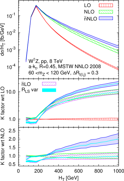
Figure 2: Differential cross sections and K factors for the effective mass observable, defined in Eq. (4), for the LHC at $\sqrt{s}=8\,\text{TeV}$. The bands correspond to varying $\mu_{F}=\mu_{R}$ by factors 1/2 and 2 around the central value from Eq. (3). The cyan solid bands give the uncertainty related to the $R_{\text{LS}}$ parameter varied between 0.5 and 1.5. The distribution is a sum of contributions from two unlike flavor decay channels, $ee\mu\nu_{\mu}$ and $\mu\mu e\nu_{e}$.

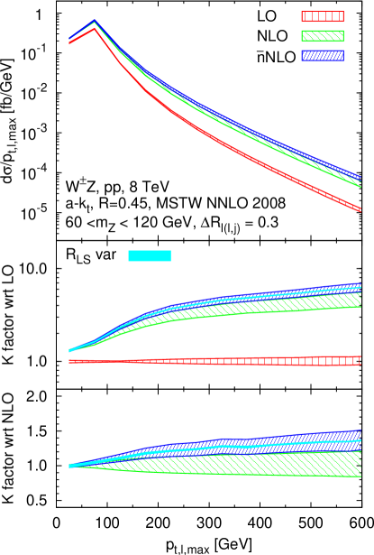
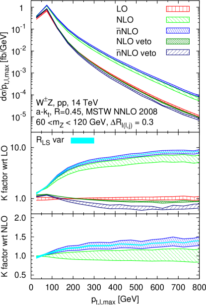
Figure 3: Differential cross sections and K factors for the $p_{T}$ of the hardest lepton for the LHC at $\sqrt{s}=8\,\text{TeV}$ (left) and $\sqrt{s}=14\,\text{TeV}$ (right). The bands correspond to varying $\mu_{F}=\mu_{R}$ by factors 1/2 and 2 around the central value from Eq. (3). The cyan solid bands give the uncertainty related to the $R_{\text{LS}}$ parameter varied between 0.5 and 1.5. The distribution are sums of contributions from two unlike flavor decay channels, $ee\mu\nu_{\mu}$ and $\mu\mu e\nu_{e}$.

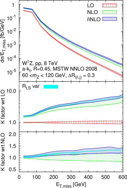
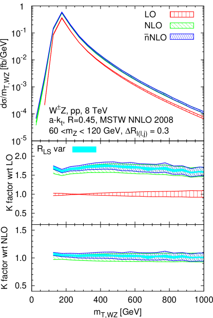
Figure 4: Differential cross sections and K factors for the missing transverse energy (left) and the transverse mass of the WZ system (right) for the LHC at $\sqrt{s}=8\,\text{TeV}$. The bands correspond to varying $\mu_{F}=\mu_{R}$ by factors 1/2 and 2 around the central value from Eq. (3). The cyan solid bands give the uncertainty related to the $R_{\text{LS}}$ parameter varied between 0.5 and 1.5. The distribution are sums of contributions from two unlike flavor decay channels, $ee\mu\nu_{\mu}$ and $\mu\mu e\nu_{e}$.

In our computations, regardless of the order, we use the MSTW NNLO 2008 Martin:2009iq PDFs with $\alpha_{s}(M_{Z})=0.11707$. We choose $m_{Z}=91.1876\,\mathrm{GeV}$, $m_{W}=80.398\,\mathrm{GeV}$ and $G_{F}=1.16637\times 10^{-5}\,\mathrm{GeV}^{-2}$ as electroweak input parameters and derive the weak mixing angle from the Standard Model tree level relations. The center-of-mass energy is fixed to $\sqrt{s}=8\,\mathrm{TeV}$ if not specified otherwise. As in the underlying VBFNLO WZ@NLO and WZj@NLO calculations, only the channels with W and Z/$\gamma^{*}$ decaying into unlike flavor leptons are considered, i.e. $pp\rightarrow W^{\pm}Z+X\rightarrow\ell_{1}^{\pm}\stackrel{{\scriptstyle\text{\tiny(}-\text{\tiny)}}}{{\nu_{1}}}\ell_{2}^{+}\ell_{2}^{-}+X$. From the theoretical perspective, to take into account all possible decay channels, i.e. $eee\nu_{e}$, $ee\mu\nu_{\mu}$, $\mu\mu e\nu_{e}$, $\mu\mu\mu\nu_{\mu}$, one can safely multiply the single flavor result by a factor four, since the Fermi interferences due to identical particles in the final state are below per mille level Campanario:2010hp . However, as explained later, we shall only apply a cut on the reconstructed mass of the opposite charge same flavor lepton pair. Therefore, all the results shown in Figs. 2–4 correspond to the sum of contributions from the two decay channels, $ee\mu\nu_{\mu}$ and $\mu\mu e\nu_{e}$. All off-shell effects are included, which takes into account spin correlations and also virtual photons. Finite width effects, related to leptonic decays of the electroweak gauge bosons, are accounted for with a fixed-width scheme Campanario:2010hp . Top quark effects are not considered and all other quarks are taken massless. Effects from generation mixing are neglected since the CKM matrix is set to the identity matrix. As the central value for the factorization and renormalization scales we choose

$$\mu_{F,R}=\frac{1}{2}\sum p_{T,\text{partons}}+\frac{1}{2}\sqrt{p_{T,W}^{2}+m_{W}^{2}}+\frac{1}{2}\sqrt{p_{T,Z}^{2}+m_{Z}^{2}}$$ (3)

where $p_{T,V}$ and $m_{V}$ have to be understood as the reconstructed transverse momenta and invariant masses of the decaying bosons. To study the impact of the QCD corrections, we choose inclusive cuts. The charged leptons are required to be hard and central: $p_{T,\ell}\geq 15(20)$, for $l$ coming from Z(W), and $|y_{l}|\leq 2.5$. The missing transverse energy must satisfy the cut $E_{T,\text{miss}}>30\,\mathrm{GeV}$. The reconstructed mass from the opposite-charge same-flavor leptons has to lie in the window $60<m_{l^{+}l^{-}}<120\,\mathrm{GeV}$, which also avoids singularities coming from off-shell photons, $\gamma^{*}\to\ell^{+}\ell^{-}$. We cluster all final state partons with $|y_{p}|\leq 5$ to jets with the anti-$k_{t}$ algorithm Cacciari:2008gp , as implemented in FastJet Cacciari:2005hq ; FastJet , with the radius $R=0.45$. For observables that involve jets, we consider only those jets that lie in the rapidity range $|y_{\text{jet}}|\leq 4.5$ and have transverse momenta $p_{T,\text{jet}}\geq 30\,\mathrm{GeV}$. In addition, we impose a requirement on the lepton-lepton and lepton-jet separation in the azimuthal angle-rapidity plane $\Delta R_{l(l,j)}>0.3$.

As a first check of our setup, we have merged WZ@LO and WZj@LO to produce WZ@$\bar{n}$LO, which can be tested against the full WZ@NLO result. In Fig. 2, we show the effective mass defined by

$$H_{T}=\sum p_{T,\text{jets}}+\sum p_{T,l}+E_{T,\text{miss}}\,,$$ (4)

which often enters in super-symmetry searches CMS-ss ; Aad:2011vj . This distribution is very sensitive to the enhancements from soft or collinear emissions of the electroweak bosons as well as to additional parton radiation coming from new channels.

In the middle panel of Fig. 2, we show the K factors with respect to the LO result and, in the bottom, the corresponding ratios to NLO. At low $H_{T}$ values, the difference between $\bar{n}$LO and NLO is at the level of 30$-40\%$. This is due to the fact that we do not have control over the finite virtual constant terms which are missing in our $\bar{n}$LO approximation. However, as the $H_{T}$ increases, the $\bar{n}$LO result converges to the full NLO, providing a prediction more accurate than a simple LO calculation. Note in the middle panel the large $\bar{n}\text{LO}$ corrections and fast convergence to the NLO result, yielding K-factors of order of 10. The $\bar{n}\text{NLO}$ corrections can be as large as 100$\%$ compared to NLO (bottom panel of Fig. 2) and they are clearly beyond the NLO scale uncertainties. We observe that the R${}_{\text{LS}}$ uncertainties are small and there is only a marginal reduction in the scale uncertainties at $\bar{n}$NLO. The latter is due to the fact that we are favoring regions of the phase space associated with new topologies entering at NNLO which are only computed at LO.

The integrated cross section for one lepton flavor, $\sigma(pp\to l_{1}\nu_{l_{1}}l_{2}l_{2})$, dominated by the low $H_{T}$ region, increases only by about 5$\%$ from 25.7 $\pm$ 1.0 (scale) fb at NLO to 26.9 $\pm$ 0.9 (scale) $\pm$ 0.4 (R${}_{\text{LS}}$) fb at $\bar{n}$NLO. We have also computed the total cross sections for 7 TeV at NLO and the result agrees with this quoted in CMS-WZ .

In Fig. 3, we show differential distributions for the lepton with maximum $p_{T}$ for $\sqrt{s}=$ 8 and $\sqrt{s}=$ 14 $\,\mathrm{TeV}$, left and right panels respectively. We observe that the $\bar{n}\text{NLO}$ corrections are large at both energies. For the 14 $\,\mathrm{TeV}$ run, these corrections are beyond the renormalization and factorization scale uncertainties above $p_{T}=$ 150 GeV. The same is true for the 8 $\,\mathrm{TeV}$ case only at slightly higher $p_{T}$. Even though the effect is less pronounced than at 14 TeV, due to the smaller relative importance of additional parton radiation, the corrections are at the 15$\%$ level already at 200 $\,\mathrm{GeV}$. In addition, for the 14 TeV case, we show the curves with a veto on the jets at NLO and $\bar{n}\text{NLO}$ where we require the absence of any jets with $p_{T}>50$ GeV. The $\bar{n}\text{NLO}$-veto corrections are negative and beyond the scale uncertainties of the NLO-vetoed predictions. This might be of relevance for anomalous coupling searches since vetoed distributions are often used to suppress additional radiation. The entire $\bar{n}\text{NLO}$-veto result has larger scale uncertainties than the NLO-vetoed curves, thus revealing, partially, accidental cancellation happening at NLO. Such a feature has been extensively discussed for jet vetoes also in the context of NNLO calculations of Higgs-boson production, e.g. Banfi:2012yh and references therein.

In Fig. 4 (left), we show the differential distributions for the missing transverse energy. We see that the $\bar{n}\text{NLO}$ corrections to this observable can be as large as the 30$\%$, exceeding the scale uncertainty of the NLO result. In the right-hand plot of Fig. 4, we show the cluster energy (transverse mass of the WZ system) defined by

$$m_{T,\text{WZ}}=\sqrt{(E_{T}^{W}+E_{T}^{Z})^{2}-(p_{x}^{W}+p_{x}^{Z})^{2}-(p_{y}^{W}+p_{y}^{Z})^{2}}\,,$$ (5)

where $E^{W,Z}_{T}$ and $p^{W,Z}_{x,y}$ are the transverse energy and the transverse momentum components of the bosons reconstructed from the four-momenta of the leptons. The $\bar{n}$NLO corrections to this observable are small, which means that this distribution is not particularly sensitive to the new topologies that appear at NNLO. For the same reason, the finite terms from the two-loop diagrams, which are missing in the $\bar{n}$NLO result, are of larger relative importance for this observable than they are for $H_{T}$, $p_{T,l,\max}$ or $E_{T,\text{miss}}$, which is also reflected in larger $R_{\text{LS}}$ uncertainties in the $m_{T,\text{WZ}}$ case.

The reason behind the marked difference in the relative size of the $\bar{n}$NLO corrections between $m_{T,\text{WZ}}$ and all the other observables which we have discussed is the following. For observables like $p_{T,l,\max}$ or $E_{T,\text{miss}}$, to receive large contributions in the high-$p_{T}$ region, it is enough that only one of the two bosons is produced at high $p_{T}$. This high-$p_{T}$ boson recoils against a high-$p_{T}$ QCD parton. The other boson can be in particular soft and collinear to a quark and such configurations, one of which is depicted in the bottom diagram of Fig. 1, come with the $\alpha_{s}^{2}\alpha_{\text{EW}}^{2}\ln^{2}\left(p_{T,j}/m_{V}\right)$ enhancement. In the case of $m_{T,\text{WZ}}$, however, the favored configurations are those in which both bosons have sizable $p_{T}$s and are preferably back to back therefore do not lead to logarithmic enhancements at NNLO.

IV Conclusions

In this letter, we have used LoopSim together with VBFNLO to compute an approximation to the NNLO QCD corrections for the process $pp\rightarrow\ell_{1}^{\pm}\smash{\stackrel{{\scriptstyle\text{\tiny(}-\text{\tiny)}}}{{\nu_{1}}}}\ell_{2}^{+}\ell_{2}^{-}+X$. Our result, referred to as $\bar{n}$NLO, is expected to be accurate in the regions of phase space dominated by the topologies other than those present at LO. As in the underlying VBFNLO WZ@NLO and WZj@NLO calculations, our treatment includes the leptonic decays of the vector bosons and all off-shell and finite-width effects.

We found that the $\bar{n}\text{NLO}$ corrections to a number of observables are sizable at high $p_{T}$ and have non-trivial kinematic dependence. It is therefore important to take them into account in searches for physics beyond the SM and other physics analyses that involve WZ production. The VBFNLO+LoopSim code is available from the authors on request and it will be made public in the near future.

References

- (1) G. Aad et al. [ATLAS Collaboration], arXiv:1208.1390 [hep-ex].
- (2) [CMS Collaboration], CMS-PAS-EWK-11-010.
- (3) G. Aad et al. [ATLAS Collaboration], Phys. Rev. D 85 (2012) 112012.
- (4) [CMS Collaboration], CMS PAS EXO-11-095.
- (5) J. Bagger, V. D. Barger, K. -m. Cheung, J. F. Gunion, T. Han, G. A. Ladinsky, R. Rosenfeld and C. P. Yuan, Phys. Rev. D 49 (1994) 1246 [hep-ph/9306256].
- (6) C. Englert, B. Jager, M. Worek and D. Zeppenfeld, Phys. Rev. D 80 (2009) 035027 [arXiv:0810.4861 [hep-ph]].
- (7) J. Ohnemus, Phys. Rev. D 44 (1991) 3477.
- (8) S. Frixione, P. Nason and G. Ridolfi, Nucl. Phys. B 383 (1992) 3.
- (9) S. Catani, L. Cieri, D. de Florian, G. Ferrera and M. Grazzini, Phys. Rev. Lett. 108 (2012) 072001.
- (10) F. Campanario, C. Englert, S. Kallweit, M. Spannowsky and D. Zeppenfeld, JHEP 1007 (2010) 076.
- (11) F. Campanario, C. Englert and M. Spannowsky, Phys. Rev. D 82 (2010) 054015.
- (12) K. Arnold, J. Bellm, G. Bozzi, F. Campanario, C. Englert, B. Feigl, J. Frank and T. Figy et al., arXiv:1207.4975 [hep-ph]; Comput. Phys. Commun. 180 (2009) 1661
- (13) M. Rubin, G. P. Salam and S. Sapeta, JHEP 1009 (2010) 084.
- (14) Y. L. Dokshitzer, G. D. Leder, S. Moretti and B. R. Webber, JHEP 9708 (1997) 001 [arXiv:hep-ph/9707323].
- (15) M. Wobisch and T. Wengler, arXiv:hep-ph/9907280.
- (16) A. D. Martin, W. J. Stirling, R. S. Thorne and G. Watt, Eur. Phys. J. C 63 (2009) 189 [arXiv:0901.0002 [hep-ph]].
- (17) M. Cacciari, G. P. Salam and G. Soyez, JHEP 0804 (2008) 063 [arXiv:0802.1189 [hep-ph]].
- (18) M. Cacciari and G. P. Salam, Phys. Lett. B 641 (2006) 57 [hep-ph/0512210].
- (19) M. Cacciari, G. P. Salam and G. Soyez, http://fastjet.fr/ .
- (20) [CMS Collaboration], CMS-PAS-SUS-12-017.
- (21) G. Aad et al. [ATLAS Collaboration], JHEP 1110 (2011) 107 [arXiv:1108.0366 [hep-ex]].
- (22) A. Banfi, G. P. Salam and G. Zanderighi, JHEP 1206 (2012) 159 [arXiv:1203.5773 [hep-ph]].