Stellar Energy Relaxation around A Massive Black Hole

Abstract

Orbital energy relaxation around a massive black hole (MBH) plays a key role in establishing the stellar dynamical state of galactic nuclei, and the nature of close stellar interactions with the MBH. The standard description of this process as diffusion in phase space provides a perturbative 2nd-order solution in the weak two-body interaction limit. We carry out a suite of $N$-body simulations, and find that this solution fails to describe the non-Gaussian short timescale evolution of the energy, which is strongly influenced by extreme events (a “heavy-tailed” distribution with diverging moments) even in the weak limit, and is thus difficult to characterize and measure reliably. We address this problem by deriving a non-perturbative solution for energy relaxation as an anomalous diffusion process driven by two-body interactions, and by developing a robust estimation technique to measure it in $N$-body simulations. These make it possible to analyze and fully model our numerical results, and thus empirically validate in detail, for the first time, this theoretical framework for describing energy relaxation around an MBH on all timescales. We derive the relation between the energy diffusion time, $t_{E}$, and the time for a small density perturbation to return to steady state, $t_{r}$, in a relaxed, single mass $n(r)\propto r^{-7/4}$ cusp around a MBH. We constrain the modest contribution from strong stellar encounters, and measure with high precision that of the weakest encounters, thereby determining the value of the Coulomb logarithm, and providing a robust analytical estimate for $t_{E}$ in a finite nuclear stellar cusp. We find that $t_{r}\simeq 10t_{E}\simeq(5/32)Q^{2}P_{h}/N_{h}\log Q$, where $Q=M_{\bullet}/M_{\star}$ is the MBH to star mass ratio, the orbital period $P_{h}$ and number of stars $N_{h}$ are evaluated at the energy scale corresponding to the MBH’s sphere of influence, $E_{h}=\sigma_{\infty}^{2}$, where $\sigma_{\infty}$ is the velocity dispersion far from the MBH. We conclude, scaling $\sigma_{\infty}$ by the observed cosmic $M_{\bullet}/\sigma_{\infty}$ correlation, that stellar cusps around lower-mass MBHs ($M_{\bullet}\lesssim 10^{7}M_{\odot}$), which have evolved passively over a Hubble time, should be dynamically relaxed. We briefly consider the implications of anomalous energy diffusion for orbital perturbations of stars observed very near the Galactic MBH.

1. Introduction

1.1. Background

Observations of our own Galactic Center (GC) reveal that stars there move on Keplerian orbits in the potential of a central compact object, which is consistent with a massive black hole (MBH) of mass $M_{\bullet}\sim 4\times 10^{6}M_{\odot}$ (Eisenhauer et al., 2005; Ghez et al., 2005, 2008; Gillessen et al., 2009a, b). It is widely assumed that the Milky Way is not unique in this sense, and that there is an MBH in the center of most, if not all, galaxies.

The GC, with its relatively low-mass MBH, represents a sub-class of galactic nuclei where the dynamical relaxation time is expected to be shorter than the Hubble time (Alexander, 2007), so that the stellar distribution near the MBH could have had time to reach a relaxed state that is independent of initial conditions. Moreover, because of its proximity, it is the only system to date where the dynamical state can be directly probed by observations. However, recent star counts in the GC (Buchholz et al., 2009; Do et al., 2009; Bartko et al., 2010) indicate that the radial density profile of the spectroscopically identified low-mass red giants on the $\sim 0.5$ pc scale, thought to trace the long-lived population there, rises inward much less steeply (or even decreases) than is expected for a dynamically relaxed stellar population (Bahcall & Wolf, 1976, 1977; Alexander & Hopman, 2009; Preto & Amaro-Seoane, 2010). The simplest interpretation is that, contrary to expectations, the GC is not dynamically relaxed by two-body interactions. This could be due, for example, to a cosmologically recent major merger event with another MBH, which carved out a central cavity in the stellar distribution (Merritt, 2010), or due to the presence of faster competing dynamical processes that drain stars into the MBH (Madigan et al., 2011).

This interpretation is however further complicated by a recent study of the diffuse light density distribution in the GC (Yusef-Zadeh et al., 2012), which is thought to track the low-mass, long-lived main-sequence stars that are too faint and numerous to be individually resolved, and consist of the bulk of the stellar mass. In contrast with the stellar number counts, the diffuse light distribution appears to rise inward rather steeply down to the $\sim O(0.01)$ pc scale, where destructive stellar collisions (not accounted for in the purely gravitational treatment of two-body relaxation), can plausibly suppress the stellar density profile (Alexander, 1999).

These uncertainties about the dynamical state of the GC, and by implication, the state of galactic nuclei in general, have far-reaching ramifications. The possibility that the GC is unrelaxed severely limits the validity of extrapolating results derived from the unique observations of the GC to other galactic nuclei. While a relaxed system can be understood and modeled from first principles, independently of initial conditions, an unrelaxed one reflects its particular formation history, which is expected to vary substantially from galaxy to galaxy. This, and the possibility that the GC lacks the predicted high-density central stellar cusp, have in particular crucial implications for attempts to understand the dynamics of extra-galactic gravitational wave (GW) sources and to predict their rates, since the low-mass MBH in the GC has long been considered the archetype of low-frequency extra-galactic targets for planned space-borne GW observatories (Amaro-Seoane et al., 2007).

The study of dynamical relaxation around a MBH has a long history, beginning with the seminal studies of Peebles (1972); Bahcall & Wolf (1976, 1977); Cohn & Kulsrud (1978); Shapiro & Marchant (1978), who used various simplifying approximations (Nelson & Tremaine, 1999) to enable analytical and numerical approaches, and continuing more recently with studies of the time to approach steady state near a MBH in large $N$-body simulations (e.g. Preto et al., 2004; Preto & Amaro-Seoane, 2010). A complementary approach of extracting the diffusion coefficients (DCs) from stellar energy evolution in $N$-body simulations was carried out in several studies (Lin & Tremaine, 1980; Rauch & Tremaine, 1996; Eilon et al., 2009; Madigan et al., 2011), leading to widely differing predictions about the dynamical state of galactic nuclei, especially very close to the MBH (Madigan et al., 2011). These open questions, and the fundamental importance of the process of orbital energy relaxation, motivate a re-examination of the analytic description of energy relaxation, coupled to detailed comparisons with carefully controlled simulations.

1.2. Objectives and overview of this study

In this study we use analytical considerations and high-accuracy $N$-body simulations to address the following open questions: What is the relation between local energy relaxation and the approach to a global steady state? What are the properties of evolution due to energy relaxation on the short and intermediate timescales? How rare are extreme energy exchange events, and what is their contribution to relaxation? What is the physical meaning, and the correct value, of the Coulomb cutoffs introduced to control the formal divergences in the relaxation rates? In practical terms, these questions all reduce to the problem of relating the analytical / statistical description of local two-body interactions, to the global measurable properties of a stellar system. These issues must be addressed in order to better understand dynamical processes in galactic nuclei, improve their modeling, and reliably apply results from $N$-body simulations to real physical systems.

Our approach to these problems is complementary to that of Preto et al. (2004). Preto et al. (2004) simulated a very large system with a non-Keplerian, and non-self-similar initial DF and potential and a relatively low mass ratio $Q=M_{\bullet}/M_{\star}$ over a relaxation timescale. Preto et al. (2004) show that there is an agreement between the $N$-body and Fokker-Planck (FP) simulations by comparing the evolution of a small inner sub-system where the potential is dominated by that of the MBH and where the analytical/ numerical solution of Bahcall & Wolf (1976) (henceforth the BW cusp) is relevant.

Here, we carry out a suite of small $N$-body simulations of a system with realistically high values of $Q$ and a potential that is dominated by the MBH, designed specifically to simplify the analytic treatment and to allow complete modeling of the time-dependent evolution on short timescales. This allows us to rigorously test and verify the theoretical predictions, and in particular the scaling of the relaxation with energy and with the slope of the cusp.

The choice of focusing on short timescales is to a large extent forced by the high computational cost of the simulations, since we model a high mass ratio system ($Q=10^{6}$, comparable to the mass ratio in the GC) with $N\geq 10^{4}$ particles which are strongly bound to the MBH. The short timescale behavior is however also of interest in itself, since dynamical processes near a MBH can be limited by the lifetime of the stars (for example, the massive stars in the GC), or by fast destructive processes (for example, collisional destruction or tidal disruption).

The elementary description of energy relaxation is by the energy transition probability, $K_{E,J}\left(\Delta E\right)$ (Eq. 24), which is the orbit-averaged probability per unit time, per unit energy, for the energy of a star to change from $E$ to $E+\Delta E$ in a single scattering event. The resulting distribution of the accumulated change in energy over a finite time $t$, $\Delta_{t}E$, is represented by the propagator, $W_{E,J}(\Delta_{t}E,t)$, which describes the energy distribution of an initially mono-energetic system of test stars, after a time $t$.

Past standard treatments of energy relaxation in stellar systems (e.g. Bahcall & Wolf, 1976) with the FP formalism implicitly assumed that only the two lowest moments of the energy transition probability (i.e. the 1st and 2nd DCs) play part in the evolution of the system. This is equivalent to assuming that the free propagator is a Gaussian with width proportional to $\sqrt{t}$, that is, energy evolves by normal diffusion. However, as we show, the $\sim 1/|\Delta E|^{3}$ divergence of the transition probability (Goodman, 1983) implies that higher order DCs do play a role, which is dominant on short timescales, and diminishes with time, but still remains non-negligible even when the system relaxes to steady state. The implications are that energy relaxation progresses somewhat faster than $\sqrt{t}$, as an anomalous diffusion process.

Our approach of measuring energy relaxation in $N$-body simulations on short timescales forces us to develop a robust statistical model for describing these timescales. By treating the problem in Fourier space, we are able to derive the full propagator explicitly. It can then be evaluated either numerically in non-perturbative form, or analytically in a perturbative manner. This enables us to show that the propagator is a heavy-tailed DF that evolves as $\sim\sqrt{t\log(t)}$ on timescales much shorter than the FP energy diffusion timescale. This short timescale behavior is an example of an anomalous diffusion process (Metzler & Klafter, 2000). One consequence is the much higher probability of events that would be expected to be extremely rare for a Gaussian probability distribution. Another implication of the very slow convergence of this propagator to the central limit is that attempts to measure relaxation in relatively short $N$-body experiments can yield very misleading results, which reflect more the method used, than the quantity probed. By analyzing the scaling properties of the energy propagator we suggest a robust statistical estimator, using fractional moments, which is independent of the high energy cutoff. With it we measure the rate of energy relaxation on short timescales and confirm our analytical treatment, and in particular, the validity of the propagator and the DCs used in the standard FP approximation. Finally, we use the propagator to evolve a system by MC simulations up to steady state, and thereby confirm the approximate validity of the FP results on long timescales.

The paper is organized as follows: In Section 2 we summarize the process of energy relaxation around a massive object in terms of a normal diffusion process described by the FP equation, and derive an analytical solution for the evolution of a stellar cusp to steady state. In Section 3 we present an elementary description of energy relaxation in terms of the transition probability and its integrated propagator, and describe the emergence of anomalous diffusion that ultimately approaches normal diffusion on long timescales. In section 4 we formulate a method to analyze our $N$-body simulations and use it to confirm and calibrate our analytical description of relaxation. In section 5 we briefly discuss the observable effects of anomalous diffusion on short period stars orbiting the Galactic MBH, perturbed by a dark cusp of stellar remnants. We summarize and discuss our results in section 6.

2. Energy relaxation as a diffusion process

The standard approach (Chandrasekhar, 1943) of treating relaxation in a self-gravitating system involves several simplifying assumptions (e.g. Nelson & Tremaine, 1999). The 2-body perturbations experienced by a test star are assumed to be independent of each other, that is, non-coherent. The encounter is assumed to be between two unbound stars, approaching each other from infinity. The perturbations are assumed to be local in two respects. (1) The exchange of energy and angular momentum occurs over a very short time at the point of closest approach. (2) The local conditions (stellar density and velocity) at the position of the test star, at the time of interaction, apply to all perturbers irrespective of their impact parameter, which is equivalent to assuming an infinite homogeneous system around the point of interaction. These assumptions cannot be satisfied for arbitrarily large impact parameters, and therefore require the introduction of a large-distance cutoff, which enters in the Coulomb factor $\Lambda$. Note however that it is far from obvious that these assumptions hold near a MBH. The potential there is dominated by the central mass, and on intermediate scales (close to the MBH, but far enough to ignore relativistic effects) is approximately Keplerian, $\phi=GM_{\bullet}/r$; the stellar density decreases steeply with radius; and there is strong energy-dependent stratification of dynamical timescales. We discuss here the implications of these factors on energy relaxation near a MBH. Finally, it is commonly assumed that this Markovian process is also a diffusive processes, and can therefore described by the FP equation.

2.1. The FP description of relaxation around an MBH

Determining the stellar distribution in the vicinity of an MBH is a classical problem in stellar dynamics, first discussed in the context of an MBH embedded in a globular cluster (Peebles, 1972; Bahcall & Wolf, 1976). The general time evolution of the phase-space distribution function (DF) of test particles with mass $m_{T}$, $f_{T}(\mathbf{v},\mathbf{x},t)$, due to two-body interaction with field stars in a local velocity-mass distribution $f_{F}(\mathbf{v},m_{F})$, is given by the master equation (Goodman, 1985)

$$\frac{D}{Dt}f_{T}(\mathbf{v},\mathbf{x},t) = \int d^{3}\mathbf{v}^{\prime}f_{T}(\mathbf{v}^{\prime},\mathbf{x},t)K(\mathbf{v}^{\prime},\mathbf{v})$$ (1)

$$-f_{T}(\mathbf{v},\mathbf{x},t)\int d^{3}\mathbf{v}^{\prime}K(\mathbf{v},\mathbf{v}^{\prime})\,,$$

where $D/Dt\equiv(\partial/\partial t)+\mathbf{v}\cdot(\partial/\partial\mathbf{x})-(\partial\phi/\partial\mathbf{x})\cdot(\partial/\partial\mathbf{v})$ and $K(\mathbf{v},\mathbf{v}^{\prime})$ is the transition probability per unit time per unit velocity volume that a test star changed its velocity from $\mathbf{v}$ to $\mathbf{v}^{\prime}=\mathbf{v}+\Delta\mathbf{v}$ as a result of a single encounter with a field star

$$K(\mathbf{v},\mathbf{v}^{\prime}) = \frac{4G^{2}}{|\Delta v|^{5}}\int dm_{F}m_{F}^{2}\int_{\mathbf{w}\cdot\Delta\mathbf{v}}d^{2}\mathbf{w}$$ (2)

$$f_{F}\left(\mathbf{w}+\mathbf{v}+\Delta\mathbf{v}\frac{m_{T}+m_{F}}{2m_{F}},m_{F}\right)\,.$$

This description of stellar dynamics as a relaxation process assumes that changes in energy and angular momentum result from uncorrelated velocity deflections, which are local in time and space (e.g. Nelson & Tremaine, 1999; Freitag, 2008). Dynamical mechanisms that involve long timescale correlations, e.g. resonant relaxation (Rauch & Tremaine, 1996), are not taken into account here.

Assume that $f_{T}$ and $f_{F}$ are functions only of orbital energy $E$ and time $t$; the potential is dominated by a massive central object $\phi=GM_{\bullet}/r$; and the field stars and the test stars have the same mass, $M_{\star}$. The master equation (1) is then reduced to an equation of energy only (here and below the energy and potential of bound stars is defined as positive),

$$\frac{\partial N(E,t)}{\partial t} = \int d\Delta E\{N(E-\Delta E)K_{E-\Delta E}(\Delta E)$$ (3)

$$-N(E)K_{E}(\Delta E)\}\,,$$

where $K_{E}\left(\Delta\epsilon\right)$ is the orbit- and eccentricity-averaged energy transition probability, and $N(E)$ is the stellar number density in energy space

$$N(E,t)=4\pi^{2}J_{c}^{2}(E)P(E)f(E,t)\,.$$ (4)

By assuming weak encounters, $\Delta E\ll E$, and expanding $N\left(E-\Delta E\right)$ and $K_{E-\Delta E}\left(\Delta E\right)$ around $E-\Delta E=E$, the master equation can be expressed as a Kramers-Moyal expansion (e.g. Weinberg, 2001)

$$\frac{\partial N(E,t)}{\partial t}=\sum\frac{1}{n!}\left(-\frac{\partial}{\partial E}\right)^{n}N(E)\Gamma_{n}^{\Lambda}\left(E\right)\,,$$ (5)

where the DCs are the moments of the transition probability $K_{E}\left(\Delta E\right)$,

$$\Gamma_{n}^{\Lambda}\left(E\right)=\int_{\Delta E_{\min}}^{\Delta E_{\max}}\Delta E^{n}K_{E}\left(\Delta E\right)d\Delta E\,,$$ (6)

and where $\Lambda=\Delta E_{\max}/\Delta E_{\min}$. For $n=1,2$, $\Gamma_{n}^{\Lambda}$ is proportional to the Coulomb logarithm $\log\Lambda$ (Eqs. 10, 11) ; for higher moments the dependence is much weaker, $\propto(1-\Lambda^{-\left\lfloor(n-1)/2\right\rfloor})$ (Eq. 31), and can usually be ignored.

By truncating the sum after the first two terms, the Kramers-Moyal expansion is reduced to the FP equation (e.g. Rosenbluth et al., 1957)

$$\frac{dN(E,t)}{dt} = \frac{1}{2}\frac{\partial^{2}}{\partial E^{2}}\{N(E,t)\Gamma_{2}^{\Lambda}(E)\}$$ (7)

$$-\frac{\partial}{\partial E}\{N(E,t)\Gamma_{1}^{\Lambda}(E)\}=-\frac{\partial F(E)}{\partial E}\,,$$

where $F(E)$ is the stellar flux.

The FP approximation is valid only if the higher order terms can be neglected. This is usually justified by arguing that the $n>2$ terms of the expansion are of the order of the $n>2$ DCs themselves, which are smaller than the first two DCs by a factor of $1/\log\Lambda$ (e.g. Binney & Tremaine, 2008; Hénon, 1960). However, as we show in Section 3.2, such a comparison is meaningful only when $\partial/\partial E\sim 1/\Delta E\sim 1/E$ (Eq. 31), i.e. the change in energy has accumulated to an order unity change. This is a valid assumption only over long timescales; on short timescales the system cannot be described by the first two DCs only.

It is further commonly assumed that stars that are unbound to the MBH ($E<0$) are drawn from a Maxwell-Boltzmann distribution,

$$f(E)=\frac{n_{0}}{\left(2\pi\sigma_{0}^{2}\right)^{3/2}}e^{E/\sigma_{0}^{2}},\quad E<0\,,$$ (8)

where $n_{0}$ and $\sigma_{0}$ are the stellar number density and velocity dispersion of this simplified model of the host galaxy. The inner energy boundary is determined by the maximal orbital energy $E_{d}$ where stars can survive against any of the various disruption mechanisms that operate in the extreme environment near a MBH (e.g. tidal disruption, tidal heating, orbital decay by gravitational wave emission, stellar collisions),

$$f(E)=0,\quad E<E_{d}\,.$$ (9)

The steady state solution ($\partial N/\partial t=0$) of the FP equation can be simply obtained if a cusp solution $f(E)=CE^{p}$ is assumed (e.g. Peebles, 1972). Although this solution does not satisfy the boundary conditions (Eqs. 8, 9), it is in fact a reasonable approximation of the full solution far from the boundaries at $0\ll E\ll E_{d}$, (e.g. Bahcall & Wolf, 1976). For a full analytic solution see Keshet et al. (2009).

Approximating the DF by a pure power-law, $-1<p<1/2$, the DCs are

$$\Gamma_{1}^{\Lambda}(E)=-\frac{4(1-4p)\log\Lambda}{1+p}\frac{N(<E)}{Q^{2}P(E)}E\propto E^{p+1}$$ (10)

and

$$\Gamma_{2}^{\Lambda}(E)=\frac{16\left(3-2p\right)\log\Lambda}{(1+p)(1-2p)}\frac{N(<E)}{Q^{2}P(E)}E^{2}\propto E^{p+2}\,.$$ (11)

The steady state solution is then (Eq. 7)

$$(4p-1)(4p-3)\frac{2}{1-2p}=0\,,$$ (12)

whose solutions are either $p=3/4$ (Peebles, 1972), which is unphysical since $\Gamma_{2}^{\Lambda}(E)$ diverges with $E_{d}\to\infty$ leading to huge stellar flux away from the MBH (Bahcall & Wolf, 1976), or $p=1/4$, the so-called BW cusp solution (Bahcall & Wolf, 1976). The BW cusp solution has zero net flow ($F=0$) since the term in the equation that contains the second DC is independent of energy, and since there is no drift (Lightman & Shapiro, 1977). This solution was confirmed by integrating the FP equation, both numerically (e.g. Bahcall & Wolf, 1976; Cohn & Kulsrud, 1978; Preto et al., 2004) and statistically (e.g. Shapiro & Marchant, 1978), by Monte-Carlo (MC) simulations.

2.2. Relaxation to steady state

Stellar systems out of equilibrium evolve by redistributing their energy and angular momentum. When this proceeds by diffusion, the timescales associated with the various DCs generally reflect the dynamical evolution timescale. One such timescale is the energy diffusion time $t_{E}$,

$$t_{E}(E)\equiv E^{2}/\Gamma_{2}^{\Lambda}(E)$$ (13)

which expresses the timescale for a test star to change its orbital energy by order unity. Another commonly used quantity is the Chandrasekhar relaxation time (Chandrasekhar, 1942; Spitzer, 1987),

$$t_{{\rm Ch}}\equiv\frac{\sigma^{2}}{\langle\left.(\Delta v_{\parallel})^{2}\rangle\right|_{v=\sqrt{3}\sigma}}=0.34\frac{\sigma^{3}}{G^{2}m^{2}n\ln\Lambda}\,,$$ (14)

where the second equality expresses the timescale for a typical test star with velocity $v=\sqrt{3}\sigma$, to change its kinetic energy by order unity, in a Maxwellian, isotropic and homogeneous stellar system with stellar mass $m$, number density $n$ and velocity dispersion $\sigma$. The Coulomb logarithm is defined by the ratio of maximal and minimal impact parameters $\ln\Lambda=\ln(p_{\max}/p_{\min})$, where $p_{\min}=Gm/\sigma^{2}$ (small angle approximation), and $p_{\max}$ is the size of the system.

These two timescales are related, but different, since $t_{{\rm Ch}}$ is local in physical space ($\mathbf{r},\mathbf{v}$), whereas $t_{E}$ is local in $(E,J)$ space, and hence is orbit-averaged over all ($\mathbf{r},\mathbf{v}$) values along the orbit, and often samples a wide range of conditions in the stellar cluster. It is therefore to be expected that the values of the two timescales can be quite different, even though they express the same basic property of the system: systems with short relaxation timescales evolve rapidly, and those with long timescales evolve slowly. For example, when the two timescale are compared at $E\sim\sigma^{2}$, typically $t_{\mathrm{Ch}}\gg t_{E}$ (Eq. 21).

The diffusive timescales cannot be used in themselves to estimate how long it takes an out-of-equilibrium system to approach steady state, assuming that such exists. This generally depends on the specific initial conditions, and the operative definition of convergence to steady state. Numeric experiments show that in many cases $t_{\mathrm{Ch}}$, evaluated at the radius of MBH influence, is a reasonable estimator for the relaxation time to steady state, $t_{r}$.

We now proceed to use the FP equation to demonstrate analytically why that is so, and to derive the relation between $t_{E}$, $t_{\mathrm{Ch}}$ and $t_{r}$ in a power-law stellar cusp around a MBH. In Section 3.3 we verify that our analysis is not limited by the approximate nature of the FP treatment, by numerically integrating the system using MC simulations where the individual energy steps are generated using the isotropic propagator $W_{E}(\Delta_{t}E)$. Moreover, we show that strong encounters, which are ignored in the FP treatment, reduce the time to reach steady state by a factor of only $\lesssim 4/3$.

Consider a background stellar population in steady state with a power-law cusp $N_{bg}(E)=(5/4)N(E/E_{p})^{-9/4}$, where $N$ is the total number of stars with $E>E_{h}$ . The DCs (Eqs. 10, 11) are $\Gamma_{1}^{\Lambda}(E)=0$ and $\Gamma_{2}^{\Lambda}(E)\propto E^{9/4}$. Assume a small initial perturbation superimposed at energy $E_{0}$ on the steady state background, $N_{p}(E)=N_{\star}\delta(E-E_{0})$. This system describes, for example, test stars that are scattered by a steady state distribution of field stars. Over time, the perturbation will spread out until it relaxes to the $\propto E^{-9/4}$ steady state distribution.

The dimensionless FP equation for the evolution of $N_{p}$ is

$$\frac{dN_{p}(x,\tau)}{d\tau} = \frac{1}{2}\frac{\partial^{2}}{\partial x^{2}}\{N_{p}(x,\tau)x^{9/4}\}\,,$$ (15)

where $x=E/E_{h}$ and $\tau=t/t_{E}(E_{h})$. We assume that the number of stars with $E>E_{h}$ is constant (i.e.  there is a reflective boundary at $E_{h}$). The perturbation then evolves as (see Eq. C11)

$$\eta(x,\tau) \equiv\frac{N_{p}(x,\tau)}{N_{p}^{\infty}(x)}\!-\!1 =\sum_{n=1}^{\infty}\!Q_{n}(x)Q_{n}(x_{0})e^{-j_{5,n}^{2}\tau/128}\,,$$ (16)

where $N_{p}^{\infty}(x)=N_{bg}(x)/N$, $Q_{n}(x)=\sqrt{x/5}J_{4}(j_{5,n}x^{-1/8})/J_{4}(j_{5,n})$, $J_{n}(x)$ is the Bessel function of the first kind and $j_{n,m}$ is the $m$’th zero of $J_{n}(x)$. Similar solutions for a power-law background cusps with $p>0$ are presented in Appendix C.

The time it takes for the small perturbation to decay, and for the system to converge back to its steady state, depends on the location of the initial perturbation, and on the operative definition of the convergence. The dynamical evolution back to steady state is slower for higher $x_{0}$ (closer to the MBH), in spite of the fact that the relaxation time decreases in that limit as $t_{E}(x)\sim x^{-p}$ ($p=1/4)$. This counter-intuitive result can be understood by considering a perturbation of mass $\Delta M$ at $x\geq x_{0}$, where the enclosed steady state mass scales as $x_{0}^{p-3/2}$. It then follows the fractional perturbation scales as $\delta M\propto x_{0}^{3/2-p}$, and the rate for relaxing the perturbation scales as $\delta M/t_{E}\propto x_{0}^{3/2}$. We therefore conservatively define the relaxation time as the time it takes a $\delta$-function perturbation in the limit $x_{0}\to\infty$ to decay to an order unity perturbation, $\eta(x_{0,}t_{r})=1$, where

$$\eta(t) = \lim_{x_{0}\to\infty}\sum_{n=1}^{\infty}Q_{n}^{2}(x_{0})e^{-j_{5,n}^{2}t/(128t_{E})}\,$$ (17)

$$\approx \frac{1}{1128\Gamma(5)^{2}}\frac{j_{5,1}^{8}}{J_{4}^{2}(j_{5,1})}e^{-j_{5,1}^{2}t/(128t_{E})}\,,$$

where here $\Gamma$ is the Gamma function. This corresponds to the relaxation time

$$t_{r}=\frac{128}{j_{5,1}^{2}}\log\left(\frac{1}{1128\Gamma(5)^{2}}\frac{j_{5,1}^{8}}{J_{4}^{2}(j_{5,1})}\right)t_{E}\simeq 11.1t_{E}\,.$$ (18)

The conclusion that $t_{r}\sim O(10)t_{E}$ is robust, since it mostly reflects the time it takes the perturbation to propagate down to $x=1$, rather than the exact details of the convergence criterion. For example, an alternative definition of $t_{r}$ in terms of evaporation, leads to a similar result. Consider the evaporation of a perturbation through the outer boundary $x=1$, and define the relaxation time to steady state as the time it takes the number of stars still in the system to decrease by a factor $P_{\star}=0.1$ (the conclusions depend only logarithmically on the exact value of $P_{\star}$). In this setting the probability to find the test star in the system is given by (see Eq. C15)

$$\frac{N_{p}(x>1,\tau)}{N_{\star}}=\frac{2}{\sqrt{x_{0}}}\sum_{n=1}^{\infty}\frac{J_{5}(j_{4,n})J_{4}(j_{4,n}/x_{0}^{1/8})}{j_{4,n}J_{5}^{2}(j_{4,n})}e^{-j_{4,n}^{2}\tau/128}\,,$$ (19)

and the relaxation time (in the limit $x_{0}\to\infty)$ is given by

$$t_{r}\approx\frac{128}{j_{4,1}^{2}}\log\left(\frac{P_{\star}^{-1}j_{4,1}^{3}}{8J_{5}(j_{4,1})\Gamma(5)}\right)t_{E}\simeq 10t_{E}\,,$$ (20)

similar to the relaxation time we obtained before.

This simple model can also explain the behavior seen in a variety of dynamical simulations of relaxation around a MBH (Bahcall & Wolf (1976) Figure 2; Hopman & Alexander (2006) Figure 1; Madigan et al. (2011) Figure 30): the initial relaxation to steady state is extremely rapid (super-exponential), while at later times it slows down to exponential decay. Eq. (17) indeed shows that the perturbation converges to steady state as a series of exponential decaying terms with progressively faster rates $128/j_{5,n}^{2}=\{0.601,\,1.19,\,1.93,\,2.81,\,3.86,\,\dots\}$. Thus, the higher terms vanish rapidly in a combined super-exponential rate, leaving last only the first and slowest term, which decays exponentially on a timescale $\gtrsim t_{E}$.

The relaxation time to steady state, $t_{r}$, can be related to the Chandrasekhar time $t_{{\rm Ch}}$ in the host galaxy (idealized here as an isotropic and homogeneous system). Beyond the MBH radius of influence at $r_{h}=GM_{\bullet}/\sigma_{0}^{2}$, where $\sigma_{0}$ is the asymptotic velocity dispersion and the stars are unbound to the MBH ($E<0$). The velocity distribution is Maxwellian, the DF is given by Eq. (8), and therefore $t_{{\rm Ch}}$ is given by Eq. (14), with the asymptotic stellar density $n_{0}$. The typical orbital energy at $r_{h}$ is $\sim\sigma_{0}^{2}/2$. Closer to the MBH, within the radius of influence where the dynamics are Keplerian, the steady state DF for bound stars with $E>\sigma_{0}^{2}$ ($\sim r_{h}/2$) is $f\approx 2f\left(0\right)\left(E/\sigma_{0}\right)^{p}$ (e.g. Bahcall & Wolf, 1976). The energy diffusion timescale is then (Eqs. 13, 11)

$$t_{E}(\sigma_{0}^{2})=\frac{1}{64}\frac{Q^{2}}{N\left(>\sigma_{0}^{2}\right)\log\Lambda}P\left(\sigma_{0}^{2}\right)\approx T_{{\rm Ch}}/44\,.$$ (21)

It then follows that $t_{r}\sim 10t_{E}\sim T_{{\rm Ch}}/4$ (Eqs. 18, 21). The large numeric pre-factors that relate these different diffusion timescales highlight the point discussed above. While these timescales all generally reflect the tendency of the system to evolve, they measure different aspects of it: $t_{{\rm Ch}}$ is a local quantity in physical space, estimated outside the evolving region; $t_{E}$ is an orbit-averaged quantity, estimated at some typical radius inside the evolving region; $t_{r}$ describes the timescale to reach global steady state. In many cases of interest, $t_{r}$ is not very different from the age of the stellar system (or the Hubble time, a commonly assumed upper limit). Inferences about the dynamical state of such systems should be mindful of the large differences between the meanings and values of the various diffusion timescales. The result $t_{r}\sim T_{{\rm Ch}}/4$ is consistent with numerical studies that show that a stellar system around a MBH approaches steady state in about $T_{{\rm Ch}}/3$ to $T_{{\rm Ch}}/2$ (e.g. Bahcall & Wolf, 1976; Hopman & Alexander, 2006).

The scaling of $t_{r}$ with MBH mass $M_{\bullet}$ can be obtained from the relation $t_{r}\simeq 10t_{E}$, the empirical $M/\sigma$ relation (Ferrarese & Merritt, 2000; Gebhardt et al., 2000; Tremaine et al., 2002),

$$M_{\bullet}=M_{0}\left(\sigma/\sigma_{0}\right)^{\alpha}\,,$$ (22)

and the stellar number parametrization $N\left(>E\right)=Q\left(E/\xi\sigma^{2}\right)^{-5/4}$, where $\xi$ is an order unity factor. The time to steady state is then $t_{r}=\left(5\sqrt{2}\pi/64\right)\xi^{-5/4}\left(M_{0}/M_{\bullet}\right)^{3/\alpha}\left(GM_{\bullet}/\sigma_{0}^{3}\right)Q/\log Q$. For $\alpha=4$, $M_{0}=1.3\times 10^{8}M_{\odot}$, and $\sigma_{0}=200\,\mathrm{km}\mathrm{s}^{-1}$ (Tremaine et al., 2002)

$$t_{r}=\left(7.8\times 10^{9}\,\mathrm{yr}\right)\xi^{-5/4}\left(\frac{M_{\star}}{M_{\odot}}\right)^{1/4}\frac{\left(Q/10^{7}\right){}^{5/4}}{\left(\log Q/\log 10^{7}\right)}\,.$$ (23)

This indicates that stellar cusps around lower-mass MBHs ($M_{\bullet}\lesssim 10^{7}M_{\odot}$ with $M_{\star}=1\,M_{\odot}$), which have evolved passively over a Hubble time, should be dynamically relaxed.

3. Beyond the diffusion approximation

3.1. Kinematic limits on energy exchange

The transition probability encodes the full description of energy evolution in the system due to 2-body encounters on all energy scales. For hyperbolic Keplerian interactions between two stars, its general form is $K_{r,E}\sim F_{r,E}(\Delta E)/|\Delta E|^{3}$, where $F_{r,E}$ is a non-diverging function of $\Delta E$, the energy change in an encounter (see Appendix A). The singularity of $K_{r,E}$ at $\Delta E\rightarrow 0$ is never reached in practice, because the finite size of the system sets a lower limit on $\Delta E$. In fact, an even stronger limit is implied by the restriction to hyperbolic orbits. A test star on an orbit with energy $E$ has radial orbital period $P(E)\sim GM_{\bullet}E^{-3/2}$ and a typical velocity $v\sim\sqrt{E}$. An encounter with another star at impact parameter $b$ leads to an exchange of energy of order $\Delta E\sim GM_{\star}/b$ and lasts a time $\sim b/v$. Since the weakest encounter that can still be approximated by a hyperbolic one, must have $b/v<P$, it follows that $\Delta E_{\min}\sim E/Q$ (i.e. $\Delta\epsilon_{\min}\sim 1/Q$ for $\Delta\epsilon\equiv\Delta E/E$) (Bahcall & Wolf, 1976). This approximate effective low-$\Delta E$ cutoff assumes that the contribution of distant and slow interactions is negligible. It is estimated below empirically by $N$-body simulations (see Section 4.2).

Kinematics introduce an inherent high-$\Delta E$ limit (Goodman, 1985). Strong encounters occur in the impulsive limit, where the distance between the test star at $r$ and the background star at $r_{b}$ is very small. The energy is then exchanged over a short time and the test star’s position remains almost fixed. In that limit, the energy one star can transfer to the other is at most its total kinetic energy. Let the test star be on an initial Keplerian orbit with semi-major axis $a$, energy $E=GM_{\bullet}/2a$ eccentricity $e$ and the eccentric anomaly $\omega$, is at radius $r=a\left(1-e\cos\omega\right)$ at the moment of the encounter. The most bound orbit it can be deflected to at fixed $r$ has $a_{\min}^{\prime}=r/2$ and $E_{\max}^{\prime}>E$. Thus, the maximal change in the relative energy of the test star is $\Delta\epsilon_{\max}^{(+)}=\max\left|E^{\prime}-E\right|/E=\left(2a/r-1\right)$. Conversely, the least bound orbit the test star can be deflected to at fixed $r$ involves kicking a background star with an initial energy $E_{b}$ to a maximally bound orbit with $a_{b}^{\prime}=r_{b}/2\approx r/2$. Since typically the least bound (or unbound) background stars have $E_{b}\sim 0$, the maximal change in the relative energy in this case is $\Delta\epsilon_{\max}^{(-)}\approx 2a/r$. Figure (1) shows the full transition probability for a specific value of $a/r$ and a power-law DF; the kinematic high-$\Delta E$ limit is clearly seen. The high-$\Delta E$ limit is ultimately set by physical (inelastic) collisions between stars of finite size, where orbital energy is not conserved due to tidal interactions, mass loss, or stellar destruction. Orbit-averaging over the phase of the test star yields $\left\langle\Delta\epsilon_{\max}^{(+)}\right\rangle=1$ and $\left\langle\Delta\epsilon_{\max}^{(-)}\right\rangle=2$, close to the commonly assumed value $\Delta\epsilon_{\max}=1$. It is interesting to note that these averaged kinematic limits are consistent with the small angle regime, conventionally defined by an impact parameter $b>2GM_{\star}/\left\langle v\right\rangle^{2}$ (e.g. Binney & Tremaine, 2008), which corresponds to $\Delta\epsilon<1$ .

Note however, that in the limit $e\rightarrow 1$, $\Delta\epsilon$ diverges, and therefore the eccentricity-averaged transition probability has finite contributions from arbitrarily large $\Delta\epsilon$. In particular, the isotropic average transition probability, and the resulting isotropic propagator, involve integrations over $\Delta\epsilon\rightarrow\infty$.

Figure 1.— The transition probability $K_{r,E}$ (Eq. A2) for the case of $a/r=1$ and a BW cusp ($p=1/4$), as function of $\Delta\epsilon$. The full transition probability (solid line) is compared to the approximate form (Eq. A3) (dashed line).

Note that the actual value of $\Delta\epsilon_{\max}$ may be lower than the kinematical one, when destructive physical collisions between stars play a role. In that case the maximal energy exchange is given by $\Delta\epsilon_{\max}^{\star}\sim 4a/QR_{\star}\approx 45\left(Q/4\times 10^{6}\right)^{-1}\left(a/\mathrm{pc}\right)\left(R_{\star}/R_{\odot}\right)^{-1}$, where $R_{\star}$ is the stellar radius. However, this is relevant only extremely close to the MBH. For example, in the Galactic center $\Delta\epsilon_{\max}<1$ for $a\lesssim 22\,\mathrm{mpc}$, and even then the effect of the collisional limit on the relaxation of the surviving stars is small; for example at $a\sim 0.22\,\mathrm{mpc}$, $\log\Lambda$ is reduced by only a factor of two.

3.2. Relaxation on short timescales

In order to measure short-timescale evolution in $N$-body simulation, it is necessary to derive the energy propagator in the short time limit. Consider a test star with an initial energy $E$ and angular momentum $J$, where the energy and angular momentum change as a result of two-body interactions over a period of time $P(E)<t<t_{E}$. In the small deflection angle limit (equivalently, $\Delta E/E<1$), the orbit averaged energy transition probability, $K_{E,J}(\Delta E)=\int d\Delta JK_{E,J}(\Delta E,\Delta J)$, can be approximated as (See Appendix A and Goodman (1983))

$$K_{E,J}(\Delta E)=\frac{\Gamma_{2}(E,J)+\Gamma_{1}(E,J)\Delta E+O(\Delta E^{2})}{2\left|\Delta E\right|^{3}}\,,$$ (24)

for $\Delta E_{\min}<|\Delta E|<E$, where $\Gamma_{2}(E,J)$ and $\Gamma_{1}(E,J)$ are given by Eqs. (A6) and (A7). Note that $\Gamma_{1,2}$ are shape parameters of the transition probability, $K_{E,J}\left(\Delta E\right)$, and are not by themselves the DCs $\Gamma_{1,2}^{\Lambda}$, which are related to them by

$$\Gamma_{1,2}^{\Lambda}\left(E,J\right)=\Gamma_{1,2}(E,J)\log\Lambda\,.$$ (25)

This distinction is important because $\log\Lambda\sim\log Q$ is typically a large, $O(10)$ factor, which is determined by our assumptions that strong encounters are ignored. Later is section 3.3 we will address this assumption and estimate the contribution of strong encounters. However we show below that the short timescales evolution of the system does not depend on the high $\Delta E$-limit.

Assume that $t$ is short enough so that the background remains fixed, and changes in $E$ and $J$ are small enough so that $K_{E,J}(\Delta E)$ is approximately constant along the trajectory of the test star in ($E$, $J$) space. Let $W_{E,J}(\Delta_{t}E,t)$ be the energy propagator. In that case the master equation is

$$\frac{\partial W_{E,J}(\Delta_{t}E,t)}{\partial t} = \int K_{E,J}(\Delta E)W_{E,J}(\Delta_{t}E-\Delta E,t)d\Delta E$$ (26)

$$-q_{2b}(E,J)W_{E,J}(\Delta_{t}E,t)\,,$$

where $W_{E,J}(\Delta_{t}E,0)=\delta(\Delta_{t}E)$ and $q_{2b}$ is the total rate at which 2-body encounters scatter the test star

$$q_{2b}\left(E,J\right)=\int d\Delta EK_{E,J}(\Delta E)=\frac{1-\Lambda^{-2}}{2\Delta E_{\min}^{2}}\Gamma_{2}(E,J)\,.$$ (27)

The energy propagator $W_{E,J}(\Delta_{t}E,t)$ can then be used to integrate the master equation in a MC scheme (e.g. Shapiro & Marchant, 1978).

The Fourier transform of Eq. (26) is

$$\left(\frac{\partial}{\partial t}-\tilde{K}_{E,J}(k)+q_{2b}(E,J)\right)\tilde{W}_{E,J}(k,t)=0\,,$$ (28)

where the solution is simply

$$W_{E,J}(\Delta_{t}E,t) = \int_{-\infty}^{\infty}\frac{dk}{2\pi}e^{ik\Delta_{t}E}e^{\left(\tilde{K}_{E,J}(k)-q_{2b}\right)t}$$ (29)

and $\tilde{K}_{E,J}(k)$ is the Fourier transform of $K_{E,J}(\Delta E)$

$$\tilde{K}_{J,E}(k) = q_{2b}-ik\Gamma_{1}^{\Lambda}-\frac{k^{2}}{2}\Gamma_{2}^{\Lambda}+\sum_{n=3}^{\infty}\frac{(-ik)^{n}}{n!}\Gamma_{n}^{\Lambda}\,,$$ (30)

where $\Gamma_{n}^{\Lambda}$ are the $n$’th (non-central) moments of $K_{J,E}(\Delta E)$. The higher odd and even moments are

$$\Gamma_{2n+1}^{\Lambda}=\frac{E^{2n}\Gamma_{1}}{2n}\frac{1-\Lambda^{-2n}}{\Delta\epsilon_{\max}^{2n}}\,,\,\,\,\,\,\Gamma_{2n+2}^{\Lambda}=\frac{E^{2n}\Gamma_{2}}{2n}\frac{1-\Lambda^{-2n}}{\Delta\epsilon_{\max}^{2n}}\,.$$ (31)

Note that Eq. (30) has an analytical expression in terms of cosine and sine integrals (see Eq. B2). Thus a full, non-perturbative, evaluation of the propagator $W_{E,J}(\Delta E,t)$ is obtained by numerically evaluating Eq. (29). This is equivalent to including in the master equation DCs of all orders (i.e. all moments of the transition probability), albeit calculated using an approximate transition probability, which incorporates the large angle limit only as an effective cutoff. This is to be contrasted with the standard FP treatment where only the first two DCs are included (often also only as approximations).

Neglecting the contribution of the $n>2$ moments in Eq. (30) results in the FP propagator

$$W_{E,J}^{FP}(\Delta_{t}E,t)=\frac{1}{\sqrt{2\pi\Gamma_{2}^{\Lambda}t}}e^{-\frac{(\Delta_{t}E-\Gamma_{1}^{\Lambda}t)^{2}}{2\Gamma_{2}^{\Lambda}t}}\,,$$ (32)

which can be related to the non-pertubative energy propagator (Eq. 29) via Eq. (30),

$$W_{E,J}(\Delta_{t}E,t) = W_{E,J}^{FP}(\Delta_{t}E,t)\left\{1+\right.\,$$ (33)

$$-\frac{1}{2}\frac{1}{3!}\frac{1}{\log\Lambda}\frac{E\Gamma_{1}}{\Gamma_{2}}\sqrt{\frac{t_{E}}{t}}H\!e_{3}\left(\frac{\Delta_{t}E-t\Gamma_{1}^{\Lambda}}{\sqrt{t\Gamma_{2}^{\Lambda}}}\right)$$

$$+\frac{1}{2}\frac{1}{4!}\frac{1}{\log\Lambda}\frac{t_{E}}{t}H\!e_{4}\left(\frac{\Delta_{t}E-t\Gamma_{1}^{\Lambda}}{\sqrt{t\Gamma_{2}^{\Lambda}}}\right)$$

$$\left.+\dots\right\}\,,$$

where $H\!e_{n}\left(x\right)$ are the Hermite polynomials and $t_{E}(E,J)=E^{2}/(\Gamma_{2}(E,J)\log\Lambda)$ is the energy diffusion time. Therefore, for $t>t_{E}/\log\Lambda$, the higher moments can be neglected, as expected from the central limit theorem.

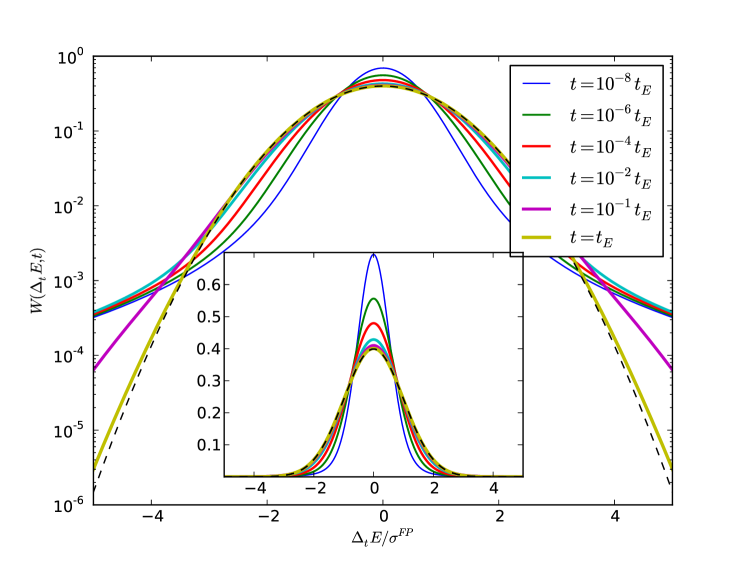
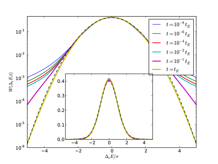
Figure 2.— Numerical evaluation of the propagator (Eq. 29) with $\Delta E_{\max}=E$ and $\Delta E_{\min}=E/10^{6}$ for several time lags (solid lines). On the left the pdf is normalized by $\sigma^{FP}=\sqrt{t\Gamma_{2}^{\Lambda}}=E\sqrt{t/t_{E}}$ as expected from the FP approximation (Eq. 32), on the right the pdf is normalized by $\sigma=\sqrt{t\Gamma_{2}^{L}(t)}$ as expected from the asymptotic analysis (first term in Eq. 34). A normalized Gaussian $\mathcal{N}(0,1)$ (dashed line) is shown for comparison. The non-perturbative propagator converges to the approximate FP one by $t\gtrsim 0.1t_{E}$. The convergence is faster in the central part of the distribution. The short timescale evolution of the central part is well approximated by a Gaussian with $\sigma=\sqrt{t\Gamma_{2}^{L}(t)}$, a clear demonstration of anomalous-diffusive evolution, which is faster than the $\sigma\propto\sqrt{t}$ of a standard random walk process.

On short timescales, the deviation from the FP propagator can be significant, as seen in Figure 2. Figure 3 shows the evolution of the energy propagator. On short timescales ($t\lesssim 0.01t_{E}$), the FP approximation overestimates the contribution of small energy changes and underestimates the contribution of large energy changes to the accumulated change. Thus, formally rare events (i.e. $>3\sigma$ for a Gaussian) have a much larger probability than expected by the FP treatment. For example, the probability of a $5\sigma$ Gaussian event ($2.9\times 10^{-7}$) can be actually as high as $1.6\times 10^{-2}$.

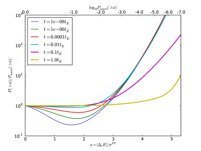
Figure 3.— The probability $P(>x)$ for a $\left|\Delta_{t}E\right|>x\sigma^{FP}$ event normalized by the probability to have such an event in a normal distribution, where $\sigma^{FP}=E\sqrt{t\Gamma_{2}^{\Lambda}}$ defined by the FP propagator. The FP propagator underestimates large $\sigma$ events, but over estimates the small $\sigma$ events.

It should be emphasized that the non-Gaussian, super-diffusive short-timescale behavior occurs in spite of the fact that the physical energy transition probability (in contrast to its simplified power-law approximation) is in fact bounded by $\Delta E_{\max}$, and therefore does have non-diverging moments. This seeming contradiction is reconciled by noting that on short timescales, this cutoff is irrelevant, since it is too far away in the wings of the distribution — the system does not evolve enough to “be aware” of its existence. This is a typical behavior for distributions whose variance would diverge were it not for physical cutoffs, for example truncated Levy-flights (e.g. Zumofen & Klafter, 1994). Only on long enough timescales, when repeated scattering populates the wings all the way to the cutoffs, does the variance converge, the conditions for the application of the central limit theorem are satisfied, and the propagator converges to its asymptotic $\sigma\propto\sqrt{t}$ behavior, independently of the functional form of $K_{E,J}(\Delta E)$.

In Appendix B we derive the effective untruncated ($\Delta\epsilon_{\max}\rightarrow\infty$) propagator $W_{E,J}^{s}(\Delta_{t}E,t)$. Since it includes arbitrarily strong energy exchanges, we refer to it at the “strong propagator” (SP). This propagator is given by a heavy tailed probability distribution

$$W_{E,J}^{s}(\Delta_{t}E,t) = W_{E,J}^{0}(\Delta_{t}E,t)+\frac{W_{E,J}^{1}(\Delta_{t}E,t)}{4\log L\left(q_{2b}t\right)}\,,$$ (34)

whose leading term is a Gaussian

$$W_{E,J}^{0}(\Delta_{t}E,t)=\frac{1}{\sqrt{2\pi t\Gamma_{2}^{L}(t)}}e^{-\frac{\left(\Delta_{t}E-t\Gamma_{1}^{L}(t)\right)^{2}}{2t\Gamma_{2}^{L}(t)}}\,,$$ (35)

where

$$\Gamma_{1,2}^{L}(t)=\Gamma_{1,2}(E,J)\log L\left(q_{2b}(E,J)t\right)\,$$ (36)

and $L\left(x\right)\approx\sqrt{e^{3-2\gamma_{E}}x}$, where $\gamma_{E}$ is the Euler constant. On long timescales approaching $t_{E}$, $L\left(q_{2b}t\right)\sim\Lambda$. The second, correction term in (34) is the higher order (in $1/\log L\left(q_{2b}t\right)$) even function that contributes an asymptotic tail of $\sim|\Delta_{t}E|^{-3}$ as $|\Delta_{t}E|\to\infty$,

$$W_{E,J}^{1}(\Delta_{t}E,t) = \frac{W_{c}^{1}\left(\frac{\Delta_{t}E-t\Gamma_{1}^{L}(t)}{\sqrt{t\Gamma_{2}^{L}(t)}}\right)}{\sqrt{t\Gamma_{2}^{L}(t)}}\,,$$ (37)

where $W_{c}^{1}(x)$ is defined in Eq. (B7). The next order odd correction function corresponds to the drift term (see Eq. B12) which is small on short timescales and is omitted here. Unlike a Gaussian, which scales self-similarly as $\sigma(t)$, the propagator in Eq. (34) is not self-similar and thus does not have a single scaling. However, its central part scales like $\sqrt{t\Gamma_{2}^{L}(t)}$, which increases with time faster than $\sqrt{t\Gamma_{2}^{\Lambda}}$, that is, in a super-diffusive manner. On longer timescales, when the cutoffs become important and the limit $\Lambda\to\infty$ is not valid, Eq. (34) is no longer a good approximation of the propagator. Note that on all timescales this approximation is valid only for some central part of the propagator and it is never a good approximation of the very far tails. Therefore this approximated propagator can not be used in the MC simulation even if the time steps of the MC are very short.

3.3. Relaxation on long timescales

The steady state configuration of a system, if such is attained on cosmologically relevant timescales, has a special significance since it is independent of the initial dynamical conditions, which are usually unknown, and is typically the most likely configuration to be observed. It is therefore important to understand how, and on what timescale, a system reaches steady state, and how short-timescale evolution by anomalous diffusion asymptotically approaches normal diffusion, as described by the FP approximation.

Table 1Summary of properties of isotropic propagators

	Strong (SP)	Exact (EP)	Weak (WP)	Fokker-Planck (FP)
Strong encounters	Overestimated	Exact	Not included
Relaxation time	$t_{r}(\mathrm{SP})\,\,\,\,\,\leq$	$t_{r}(\mathrm{EP})\,\,\,\,\,\leq$	$t_{r}(\mathrm{WP})\,\,\,\,\,=$	$t_{r}(\mathrm{FP})$
Moments	All diverge	Only $n=1,2$ finite	All finite	$n=1,2$ finite, $n>2$ zero
Gaussianity	Only central part, $\sigma^{2}\sim t\log t$	On long timescales, $\sigma^{2}\propto t$		Always, $\sigma^{2}\propto t$

On short timescales, rare strong encounters ($\Delta\epsilon>1$) can be neglected. However, as time progresses, even these rare events contribute significantly, and the kinematic limit (Section 3.1) must be taken into account. A key issue is to estimate their effect on the relaxation rate. In principle, the exact propagator (EP) provides a full description of all encounters. However, from a practical point of view it is difficult to implement it in an analytical or numerical scheme, due to the required triple integration (but see Goodman 1983). Instead, as we show below, the EP can be bracketed by two limiting approximations. The first, the SP $W_{E}^{s}(\Delta_{t}E)$ (Eq. 34), over-estimates the contribution of strong encounters by taking the weak-limit transition probability (Eq. 24), and integrating it to $\Delta\epsilon_{\max}\rightarrow\infty$, i.e. beyond the weak limit (Eq. B2). The second, the weak propagator (WP) $W_{E}(\Delta_{t}E)$, integrates only up to $\Delta\epsilon_{\max}=1$, where the weak limit is valid (Eq. 30). As argued below (see Figures 4, 5), the SP, WP and FP propagator all lead to evolution to the same steady state, on similar timescales. This then proves that so must the EP, and that the contribution of strong encounters to reaching steady state is not crucial. Table 1 summarizes the properties of the four isotropic propagators that enter our analysis of relaxation.

The inclusion of strong encounters in the transition probability can only accelerate relaxation. Therefore, the SP is expected to lead to the fastest relaxation, followed by the EP, while the WP and the FP are slowest, since they assume the weak limit. The question of the existence and values of the moments of the propagators reflect the form assumed for the transition probability, and in turn are related to the nature of the long-term evolution of the system. The weak limit assumption introduces a cutoff on the energy exchange, which ensures that all moments exist. In particular, the neglect of all $n>2$ moments assumed for the FP propagator, implies that it must be a Gaussian. Both the WP and the exact one are guaranteed by the Central Limit Theorem to converge to a Gaussian. The WP, by construction ($\Delta\epsilon_{\max}=1$) converges to the FP Gaussian. This is not the case for the EP, which takes into account the actual kinematic limits. These can be shown to correspond in the asymptotic (Gaussian) long timescale limit to an effective $\Delta\epsilon_{\max}^{\mathrm{eff}}\gg 1$. However, as we demonstrate below (Eq. 39), this limit is approached only on timescales much longer than the time for the stellar system to relax to steady state, and therefore has little effect on the actual time to reach steady state. This even holds for the SP ($\Delta\epsilon_{\max}\to\infty$), where all the moments diverge and the propagator never converges to a Gaussian with width $\propto\sqrt{t}$.

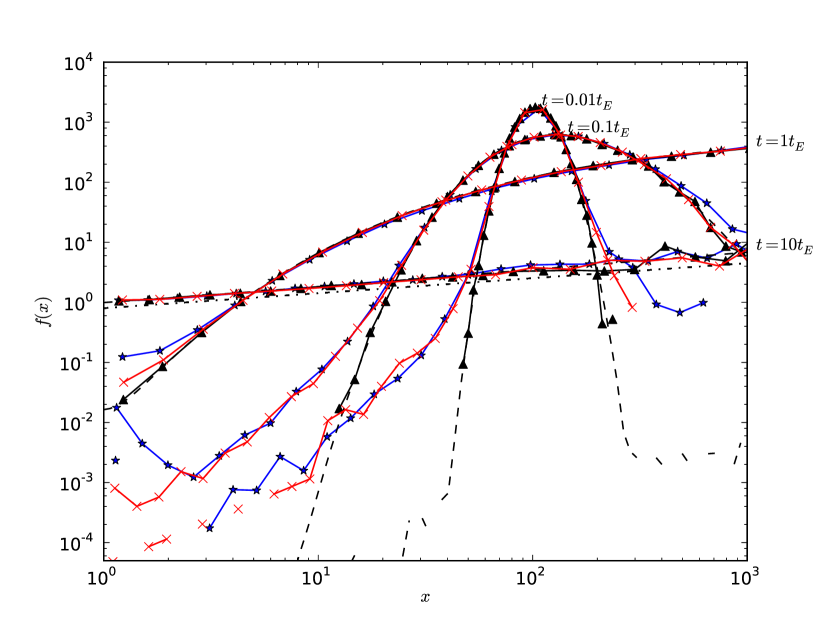
Figure 4.— Time evolution of the perturbation’s DF $f_{p}(x,t)$ for initial perturbation at $x_{0}=100$. The system is integrated by MC, with individual energy steps drawn from the FP propagator (triangles), the isotropic WP $W_{E}(\Delta_{t}E)$ (crosses), and the isotropic SP $W_{E}^{s}(\Delta_{t}E)$ (asterisks). The analytically derived DF $f_{p}(x,t)$ (Eq. 16) is shown for comparison (solid lines). All propagators converge to the FP DF for $t>t_{E}$. The asymptotic steady state $f_{p}(x)\propto x^{1/4}$ is also shown for reference (dash-dotted line).

The long-term evolution of the system can be described by repeated application of the propagator on short-enough timescales. Computationally, this can be realized by a MC simulation, which follows the evolution of the orbital energy of individual stars as it changes by small random increments, drawn from the distribution function described by the propagator. Figure 4 shows snapshots from a set of such simulations. In each, a different propagator is used to follow the evolution of an initial $\delta$-function distribution of test stars around a MBH, assuming a relaxed stellar background, and a reflecting boundary condition at the outer edge of the system. In all cases, the perturbation relaxes to the steady-state BW solution after $t_{r}\sim 10t_{E}$. This provides numeric validation of the analytical treatment of this process (Section 2.2). As expected, the evolving DFs resulting from the WP and SP are significantly broader at early times than the FP one. This reflects their heavy-tailed probability distributions (e.g. Figure 2).

Another demonstration of the near equivalence of the different propagators is shown in Figure 5. where the different propagators are used to follow the evolution of an initial $\delta$-function distribution, assuming an absorbing boundary condition at the outer edge of the system. In this configuration, the time to relaxation can be defined as the time it takes the system to evaporate some large fraction of its stars. Since we are interested here mainly in comparing the evolution due to the different propagators, our conclusions do not depend on the exact fraction. For definitiveness, we choose $0.9$. Both the FP and the WP drive evaporation on almost the same timescale, while the SP drives it only slightly faster, by a factor of $\sim 1.1$ (for $\Delta\epsilon_{\min}=Q^{-1}=10^{-6}$).

This modest acceleration in the evaporation rate by the SP, despite the inclusion of arbitrarily strong encounters, can be explained by the fact that the system evolves to its steady state much faster than the rate at which $\Delta\epsilon>1$ events contribute to relaxation. This can be shown in a quantitative way by defining an effective, time-dependent diffusion timescale for the SP.

On long timescales, the SP is dominated by its central Gaussian, and therefore its width, $\sigma^{2}=t\Gamma_{2}\log\left[L\left(q_{2b}t\right)\right]$ (Eq. 34), can be used to estimate an instantaneous diffusion timescale, $t_{E}^{\mathrm{ins}}(t)=E_{\min}^{2}/\Gamma_{2}\log L(q_{2b}t)$. Therefore, at time $t$, the evolution of the system up to this time can be described by the FP equation with an effective (time-averaged) diffusion time

$$\frac{1}{t_{E}^{\mathrm{eff}}\left(t\right)}=\frac{1}{t}\int_{0}^{t}\frac{1}{t_{E}^{\mathrm{ins}}(t^{\prime})}dt^{\prime}$$ (38)

The analytic solution of the FP equation (see Section 2.2), $t_{r}\approx 10t_{E}(E_{\min})$ then suggests to associate the time for relaxation to steady state by the SP with the solution of the ansatz $t_{r}\approx 10t_{E}^{\mathrm{eff}}(t_{r})$,

$$t_{r}^{SP}\approx 10E_{\min}^{2}\left/\left[\Gamma_{2}\left(E_{\min}\right)\log\left(\sqrt{10}e^{3/2-\gamma_{E}}/\Delta\epsilon_{\min}\right)\right]\right.\,,$$ (39)

which corresponds to an effective $\Delta\epsilon_{\max}=\sqrt{10}e^{3/2-\gamma_{E}}\approx 8$. This implies that by time $t_{r}$, the SP can be represented by an FP propagator with a Coulomb logarithm that is formally increased to $\approx\log(8/\Delta\epsilon_{\min})$ (Figure 5), thereby providing a lower limit on the time to relaxation due to the inclusion of strong encounters, $t_{r}\gtrsim t_{r}^{FP}\log(1/\Delta\epsilon_{\min})/\log(8/\Delta\epsilon_{\min})$.

This lower limit is to be compared to the time for relaxation that can be formally defined for the EP through its $\Gamma_{2}^{\Lambda}$ diffusion coefficient, where for the $p=1/4$ cusp, $\Lambda\approx 56/\Delta\epsilon_{\min}$ (see Eq. A16). Assuming that the EP has already converged to the diffusive limit, this then implies that $t_{r}^{EP}/t_{r}^{SP}\approx\log(8/\Delta\epsilon_{\min})/\log(56/\Delta\epsilon_{\min})<1$. This is in contradiction with $t_{r}^{SP}$ being the lower limit on the time to relaxation, which means that the EP does not reach the diffusive limit by time $t_{r}$, and therefore cannot be fully described by an FP equation. Nevertheless, the FP equation remains a reasonable approximation for describing relaxation around a MBH, since the discrepancy in timescales is not very large. For example, for $\Delta\epsilon_{\min}=Q^{-1}$ (Section 3.1), $0.76<t_{r}^{FP}/t_{r}^{SP}<0.92$ in the range $Q=10^{3}-10^{10}\,M_{\odot}$.

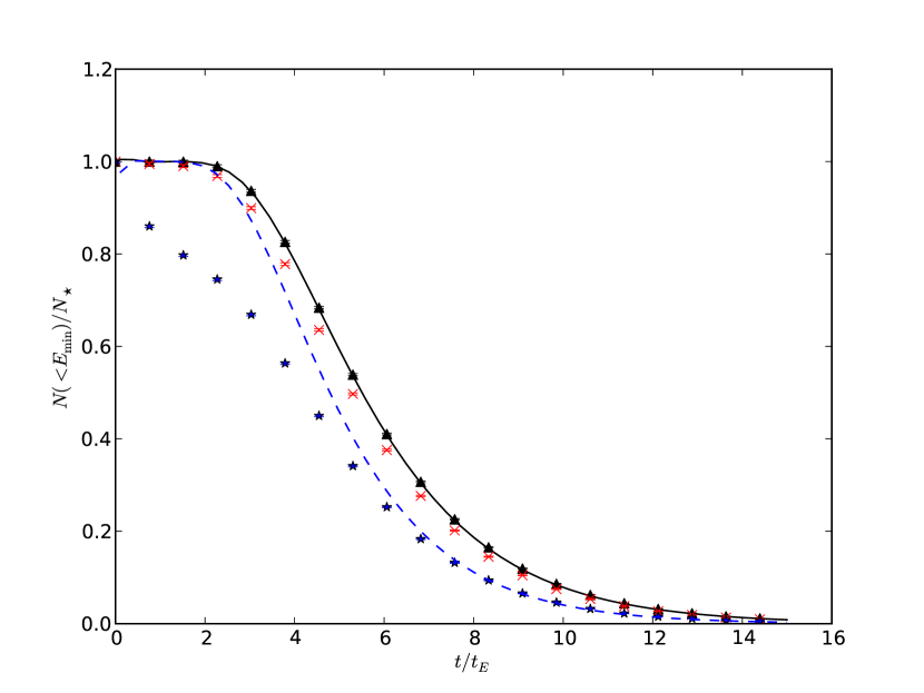
Figure 5.— Time evolution of the perturbation’s $N_{p}\left(x>1\right)/N_{\star}$ for initial perturbation at $x_{0}=10^{5}$ as a function of time. The system is integrated by MC, with individual energy steps drawn from the FP propagator (triangles), the isotropic WP $W_{E}(\Delta_{t}E)$ (crosses), and the isotropic SP $W_{E}^{u}(\Delta_{t}E)$ (asterisks). The analytically derived $N_{p}\left(x>1\right)/N_{\star}$ (Eq. 19) is shown for comparison (solid line). The analytically derived $N_{p}\left(x>1\right)/N_{\star}$ (Eq. 19) with $\Delta\epsilon_{\max}^{\mathrm{eff}}=e^{3/2-\gamma_{E}}\sqrt{10}$ is shown for comparison (dashed line).

4. Measuring energy relaxation

4.1. Overview of the best fit procedure

The propagator $W_{E,J}(\Delta_{t}E,t)$ (Eq. 29) is determined by the shape of the stellar cusp through the known functions $\Gamma_{1}(E,J)$ and $\Gamma_{2}(E,J)$ (Eqs. A6, A7), and by the parameters $\Delta\epsilon_{\min}$ and $\Delta\epsilon_{\max}$. However, on the short timescales accessible through our $N$-body simulations, the propagator is fully determined by $\Gamma_{1}$, $\Gamma_{2}$ and the parameter $\Delta\epsilon_{\min}$ only (see Eq. 34). In practice, $\Gamma_{1}(E,J)$ has a vanishing contribution to energy relaxation on short timescales, so that the propagator can be approximated as a functional of $\Gamma_{2}$ with one free parameter, $\Delta\epsilon_{\min}$.

As shown below, careful analysis of the $N$-body results reveals that the propagator model provides an excellent description of the data (Figures 7 and 8). We thereby validate the functional form of $\Gamma_{2}$, and determine the value of $\Delta\epsilon_{\min}$. In principle, if it were also possible to validate $\Gamma_{1}$ and determine $\Delta\epsilon_{\max}$, then the full shape and range of the transition probability (Eq. 24) could be determined, and the DCs $\Gamma_{1,2}^{\Lambda}=\Gamma_{1,2}(E,J)\log\Lambda$ could be calculated reliably. As it is, we have to rely on the fact that both $\Gamma_{1}$ and $\Gamma_{2}$ were derived in the same theoretical framework, and therefore assume that the excellent fit for $\Gamma_{2}$ also implies a validation of $\Gamma_{1}$. Furthermore, since in the small deflection angle limit $\Delta\epsilon_{\max}\sim O(1)$, setting $\Delta\epsilon_{\max}=1$ is expected to have only a small effect on the numerical value of $\log\Lambda=\log\left(\Delta\epsilon_{\max}/\Delta\epsilon_{\min}\right)$. We find that with this empirically-motivated calibration, the numerical values of the DCs lie within $\lesssim 20\%$ of their theoretically predicted values.

4.2. Analysis of the $N$-body results

To test and calibrate the analytic formulation of energy relaxation, we carried out a suite of Newtonian $N$-body simulations. Each simulation consisted of $10^{4}$ stars of equal mass $M_{\star}$, and a central massive object of mass $M_{\bullet}=10^{6}M_{\star}$. The initial semi-major axes of the stars were drawn from a $\rho(a)da\propto a^{2-\gamma}da$ distribution for $\gamma=1.0$, $1.25$, $1.5$ and $1.75$, with random phases and isotropic orientations. The initial eccentricities were drawn from an isotropic $\rho(e)de=2ede$ distribution. In the Keplerian limit, these models approximately correspond to a power-law density cusp, $n(r)\propto r^{-\gamma}$. The simulations were carried out with the parallel Nbody6++ code (implementing Hermite integration with hierarchical block time steps, the Ahmad-Cohen neighbor scheme for efficient calculation of accelerations, and the Kustaanheimo-Stiefel regularization method for dealing with close few-body sub-systems) (Spurzem et al., 2001; Khalisi & Spurzem, 2006).

Measuring energy relaxation in short-timescale $N$-body simulations is challenging, since the distribution of energy jumps is heavy-tailed, but the large energy exchange cutoff is not reached on these timescales (Section 3.2). Consequently, commonly used measures of evolution, such as the rms of the energy change, are strongly affected by rare strong exchanges and do not offer a robust characterization of the evolving energy distribution. After some experimentation, we adopted a statistically robust method, described below, whose key idea is to estimate the width of the central Gaussian component of the energy distribution as the limit of fractional moments.

Snapshots of the $N$-body simulation results are recorded at equally spaced times $\{t_{i}=i\delta t\}_{i=0,1,2,\ldots}$. For each star $n$ of the total $N$, the orbital energy at $t_{i}$, $E_{i}^{n}$, is calculated and recorded. The stars are assigned to logarithmically-spaced energy bins by their initial orbital energy. For each star, and for each time-lag $\{\Delta t_{k}=k\delta t\}_{k=1,2,3,\ldots}$, the relative energy changes are collected on non-overlapping, consecutive intervals: $\{\Delta\epsilon_{k}^{n}\}=\{(E_{i+k}^{n}-E_{i}^{n})/E_{i}^{n}\}_{i=0,k,2k,3k,\ldots}$, thereby avoiding the complications of statistical inter-dependencies and correlations. The measured relative energy differences, $\{\Delta\epsilon_{k}^{n}\}$, are drawn from the heavy-tailed parent distribution $W_{E_{i},J_{i}}(\Delta\epsilon_{k}^{n},\Delta t_{k})$, whose characteristic parameters need to be estimated from the numerical data. We use the fact that the central part of $W(\Delta\epsilon,t)$ is Gaussian to a good approximation with a scale parameter $\sigma_{\Delta E}^{2}(t)=t\Gamma_{2}^{L}(t)$ (Eq. 34). Since most of the data lies within the central Gaussian (Figure 8), its width can be robustly measured. As shown in Appendix B, the scale parameter can be robustly estimated by fractional moments $\delta<1$ (e.g. Zumofen & Klafter, 1994), which give a larger weight to the central part of the distribution and a smaller one to the diverging tails,

$$\sigma_{\Delta E}^{2} (t)= \lim_{\delta\to 0}\frac{\langle|E(0)-E(t)|^{\delta}\rangle^{2/\delta}}{2\pi^{-1/\delta}\Gamma\left(\frac{1+\delta}{2}\right)^{2/\delta}}\,,$$ (40)

where $\Gamma(x)$ is the Gamma function and we assumed that $W_{E_{i},J_{i}}(\Delta\epsilon,t)$ is symmetric since in our case, $t\Gamma_{1}^{2}\ll\Gamma_{2}$ (negligible drift). In particular, this relation also holds for a pure Gaussian (for any $\delta$). We verified that the results converge rapidly as $\delta\rightarrow 0$; the results below are estimated with $\delta=10^{-3}$.

Over the short timescales of our simulations, $E$ and $J$ for each star can be approximated as fixed at their initial values $E_{\star}$, $J_{\star}$. Using Eq. 40, we define for each star a dimensionless scale parameter, which we measure directly from the data,

$$\sigma_{\Delta\epsilon,\star}^{2}=\frac{\Gamma_{2}^{L}(E_{\star},J_{\star},\tau P_{\star})\tau P_{\star}}{E_{\star}^{2}}=\lim_{\delta\to 0}\frac{\langle|\Delta\epsilon_{i,k}|^{\delta}\rangle^{2/\delta}}{2\pi^{-1/\delta}\Gamma\left(\frac{1+\delta}{2}\right)^{2/\delta}}\,,$$ (41)

where $\Delta t_{k}=\tau P_{\star}$, $P_{\star}=P(E_{\star})$ and we use the minimal lag $\tau=1$ in order to obtain maximal statistics (Figure 6).

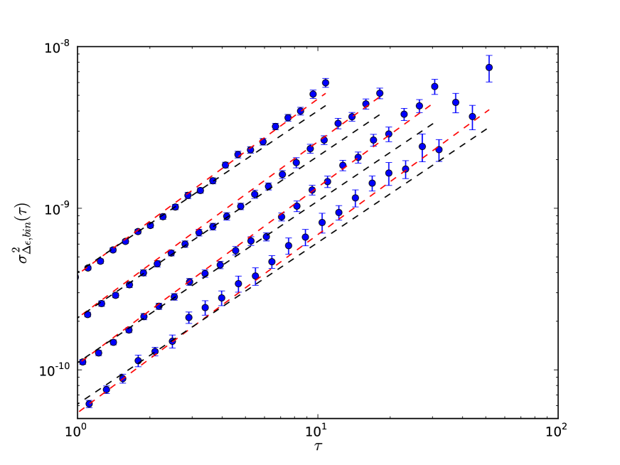
Figure 6.— The evolution of the energy scatter $\sigma_{\Delta\epsilon,\mathrm{bin}}^{2}(\tau)$ (Eq. 42) (blue circles) in $N$-body simulations for several energy bins (displayed shifted on the $y$-axis for convenience). On time-lags $\tau>1$ the scatter grows as $\tau\log\tau$ (red dashed lines), as expected from our analysis. This is somewhat faster than the $\propto\tau$ rise expected for normal diffusion (black dashed lines).

We choose the energy bins to be wide enough so that the bin average over $J$ is close enough to the isotropic average. Using Eq. (41), we define the bin averaged dimensionless scale parameter

$$\sigma_{\Delta\epsilon,\mathrm{bin}}^{2}(\tau) \equiv \left\langle\frac{\Gamma_{2}^{L}(E_{\star},J_{\star},\tau P_{\star})\tau P_{\star}}{E_{\star}^{2}}\right\rangle_{{}_{bin}}$$ (42)

$$\approx \frac{\Gamma_{2}(E_{bin})\tau P_{\mathrm{bin}}}{E_{\mathrm{bin}}^{2}}\log L\left(\frac{\tau P_{\mathrm{bin}}\Gamma_{2}(E_{\mathrm{bin}})}{2\Delta\epsilon_{\min}^{2}E_{\mathrm{bin}}^{2}}\right)\,,$$

where $E_{bin}$ and $P_{bin}$ are the bin averaged values. The second approximate equality relates the measured quantity to the theoretical model (Eq. 36), under the assumption that the weak dependence of $\log L(x)$ on $x$ allows $\left\langle x\log L(x)\right\rangle_{\mathrm{bin}}$ to be approximated by $\left\langle x\right\rangle_{\mathrm{bin}}\log L\left(\left\langle x\right\rangle_{\mathrm{bin}}\right)$ . Finally, we calculate $\Gamma_{2}$ from Eq. (D2), and fit $\sigma_{\Delta\epsilon,\mathrm{bin}}^{2}$ to the $N$-body data to obtain the best fit estimate of $\Delta\epsilon_{\min}$ and a goodness of fit score for the model (Figure 7).

Our estimated best fit values for $\Delta\epsilon_{\min}$, averaged over $\sim 10$ simulations each for various values of the power-law cusp, are presented in Table 2. We also list the relative errors resulting from the simple approximation $\Lambda=Q$, assuming $\Delta\epsilon_{\max}=1$. Figure 6 shows the growth of the width of the central Gaussian, $\sigma_{\Delta\epsilon,\mathrm{bin}}^{2}$ as function of the time-lag $\tau$. Pure diffusion would lead to a $\propto\tau$ behavior at $\tau>1$. However, the clear trend of a steeper than linear growth $\sim\tau\log\tau$, a signature of anomalous diffusion.

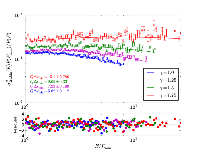
Figure 7.— The energy diffusion rate as measured by $\sigma_{\Delta\epsilon,\mathrm{bin}}^{2}\left(\tau=1\right)P(E_{\min})/P\left(E_{\mathrm{bin}}\right)$ as a function of $E_{\mathrm{bin}}/E_{\min}$ for different cusps. The analytical prediction (solid lines) is fitted to the measured values in the $N$-body simulations (dots), using $\Delta\epsilon_{\min}$ as a free parameter (see Eq. 42).

Table 2Measured $\Delta\epsilon_{\min}$

$\gamma$	$\bar{\Delta\epsilon}_{\min}/Q^{-1}$ (1)	$\bar{\Lambda}/Q$ (1,2)	$\overline{\log\Lambda}/\log Q$(1,2)	$\overline{\chi_{\mathrm{red}}^{2}}(\bar{\Delta\epsilon}_{\min})$	$n_{\mathrm{sim}}$
$1.0$	$5.3\pm 0.5$	$0.19\pm 0.02$	$0.88\pm 0.01$	$1.2\pm 0.3$	$8$
$1.25$	$6.7\pm 0.7$	$0.15\pm 0.02$	$0.86\pm 0.01$	$1.3\pm 0.2$	$12$
$1.5$	$9.2\pm 1.3$	$0.11\pm 0.02$	$0.84\pm 0.01$	$1.5\pm 0.5$	$9$
$1.75$	$13.7\pm 3.6$	$0.07\pm 0.02$	$0.81\pm 0.02$	$2.0\pm 0.6$	$9$
1 For $Q=10^{6}$, best fit values for $N$-body results (Section 4.2).
2 $\bar{\Lambda}=\Delta\epsilon_{\max}/\bar{\Delta\epsilon}_{\min}$, where $\Delta\epsilon_{\max}=1$

Finally, to verify our analysis we plot the histogram of the orbital energy jumps $\Delta\epsilon_{i,k}$ in a given energy bin and compare it to the bin-averaged propagator

$$W_{E_{\mathrm{bin}}}(\Delta\epsilon,t) \simeq \left\langle W_{E_{\star},J_{\star}}(\Delta\epsilon,t)\right\rangle_{E_{\mathrm{bin}}},$$ (43)

where we evaluated $W_{E_{\star},J_{\star}}(\Delta\epsilon,t)$ numerically for each star using the fitted $\Delta E_{\min}$, and Eq. (A7). An example is shown in Figure 8. For comparison we also show the expected bin-averaged FP propagator $\langle W_{E_{\star},J_{\star}}^{FP}(\Delta\epsilon,t)\rangle$ and the bin- averaged central Gaussian of the short timescale propagator (Eq. 34).

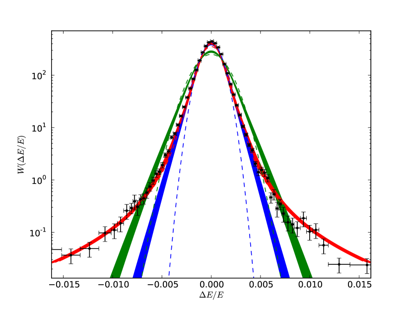
Figure 8.— The distribution of energy jumps (gray crosses) measured in the $N$-body simulations, at one energy bin. Red strip: exact numerical evaluation of the full propagator (Eq. 29), for the range of stellar angular momenta in the bin. Blue strip: the central Gaussian of the full propagator (first order term in Eq. 34). Green strip: the FP propagator (Eq. 32).

5. Application example: Stellar orbits around the Galactic MBH

The dynamical effects of stellar encounters between stars in the GC may be detectable by next-generation telescopes (e.g. Weinberg et al., 2005; Bartko et al., 2009), and be used to probe the existence of the hypothesized stellar cusp there. Since the relaxation time in the inner GC is many orders of magnitude longer than the $O(10\,\mathrm{yr})$ observational timescale, such encounters will be in the anomalous diffusion regime.

The question of the existence of the dark cusp near the MBH is closely tied to the puzzling paucity of the old luminous giants there, whose absence is in contradiction to the theoretical expectation for an old relaxed system (Bahcall & Wolf, 1976, 1977; Alexander & Hopman, 2009). A possible explanation is that a relaxed cusp does exist there, but for some reason, for example the selective destruction of extended giant envelopes (e.g. Alexander, 1999), the old giants do not trace the overall population. In that case the cusp is dark, that is, composed mainly of compact remnants and faint low-mass stars, and is expected to be dominated by $\sim 10\,M_{\odot}$ stellar mass black holes that have accumulated by the process of strong mass segregation over cosmological times (Alexander & Hopman, 2009).

Changes in orbital energy can be expressed as changes in the radial orbital period (equivalently, a phase drift). Assuming that the dominant cause of such changes is 2-body interactions, or that it is possible to model and subtract all other competing effects, then one way of detecting or constraining the dark cusp is through the stochastic orbital phase drift in the few observed luminous stars very close to the MBH.

Figure 9 shows the probability of a period change $dP/P$ after $10$ years for a test star with an orbital period of one year (semi-major axis of $0.7$ mpc), as a result of interacting with a relaxed main sequence cusp ($\rho(r)\sim r^{-7/4}$) and with a mass-segregated dark cusp ($\rho(r)\sim r^{3/2+p}$) of stellar remnants. Figure 10 shows that a change of $dP/P=0.0015$ over 10 years due to a mass segregated dark cusp, measurable by next-generation telescopes, has a non-negligible probability of $\approx 3.3\%$ per star. It should be noted that assuming only the effects of strong single encounters leads to an under-estimate of the probability (1.5%) of such an event, while the FP probability of $10.5\%$ is an over-estimate, because the event lies at the relatively under-populated intermediate wings of the propagator (Figure  9). The naive FP estimate could therefore lead to erroneous conclusions about the absence of a cusp in the case of a null result. For example, if an event of $dP/P=0.0015$ is detected, the FP $\left\{1,2,3,4,5\right\}\sigma$ confidence levels on the minimal number of stars in the cusp, $\min_{n\sigma}N_{FP}$, will differ from the true ones (due to anomalous diffusion), $\min_{n\sigma}N$, by factors $\min_{n\sigma}N_{FP}/\min_{n\sigma}N=\left\{0.52,0.55,1.7,38,2.7\times 10^{3}\right\}$, respectively. Thus, the erroneous assumption of normal diffusion may result in either over- or under-estimates of the dark cusp density, depending on the chosen confidence level.

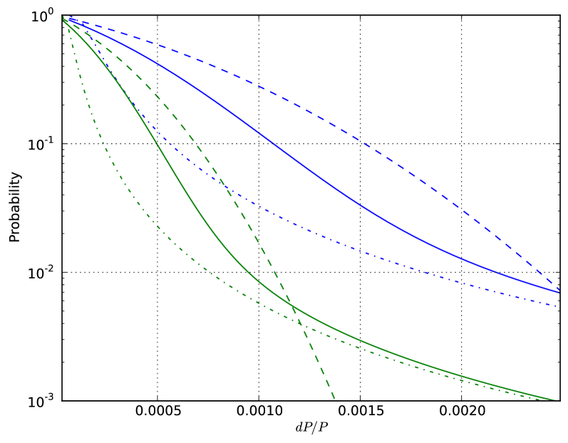
Figure 9.— Probability for a change in the orbital period of a star with a $1$ year period, over an observation time of $10$ years, for several background population models. The probability for an accumulated period change due to multiple energy changes calculated by the short time propagator (Eq. 29) (solid lines), is larger than the probability for this change due to a single energy scatter (dash-dotted lines). For comparison, we show the accumulated period change probability calculated by the FP propagator (dashed line). The background population is modeled by a cusp of $1M_{\odot}$ stars with a slope of $\gamma=1.75$ (green) with a total mass of $10^{6}M_{\odot}$ within $1$ pc, and by a cusp of $10M_{\odot}$ stellar remnants with a slope of $\gamma=1.9$ (blue) and a total mass of $10^{5}M_{\odot}$ within $1$ pc.

Figure 10.— Visualization of the orbital perturbation of a one year Keplerian orbit with an eccentricity of $0.9$ to a level of $\Delta P/P=0.0015$ (blue), $0.003$ (green) and $0.006$ (red), sampled on equal times, with respect to the original period (black). The maximal spatial shifts are $0.415$ mas, $0.824$ mas and $1.61$ mas.

6. Discussion and summary

The stochastic evolution of a stellar system is described at the most basic level by the transition probability, which expresses all the physical processes considered, and all the approximations assumed. The accumulated effect of multiple scattering events over a time that is short enough for the system to remain almost unchanged, is constructed by integration over the transition probability, and is described by the propagator. This general description of the short- or medium-term evolution can lead to a wide range of stochastic processes. Only in the specific case when the propagator asymptotes to a Gaussian, which is fully defined by its two first moments (the first and second DCs), does the evolution progress as $\propto\sqrt{t}$ and the process becomes normal diffusion, which is described by the FP equation. However, it is not at all guaranteed that this convenient and useful limit provides a valid description of the accumulated effects of the transition probability—this has to be proved case by case. There are in fact many examples of anomalous diffusive processes, whose origins can be traced to divergences of the moments of the transition probability, such as the super-diffusive Levy flights (e.g. Metzler & Klafter, 2000)

The FP equation has been applied extensively in past studies of nuclear dynamics near a MBH. However, the simplifications, assumptions and free parameters (many necessitated by the diverging, un-screened nature of the gravitational force), which are needed to justify and use this method, remained largely untested. This called for a more rigorous validation of the basic underlying assumptions. This need was further motivated by some conflicting theoretical and numerical results on the emerging timescales of diffusion and relaxation in galactic nuclei (e.g. Bahcall & Wolf, 1976; Preto et al., 2004; Merritt, 2010; Madigan et al., 2011). These impact multiple issues of interest: the rates of tidal disruptions, the rates of GW emission events from inspiralling compact objects, and the stellar distributions very close to MBHs, and in particular those of compact remnants and stars on relativistic orbits. Furthermore, the one system where the stellar distribution around an MBH can be directly observed, the GC, does not follow the FP predictions for an isolated old population, in contrast to prior expectations (Buchholz et al., 2009; Do et al., 2009; Bartko et al., 2010; Merritt, 2010).

Past studies of relaxation theory usually bypassed the use of the transition probability (but see Goodman, 1983). They assumed from the outset that the diffusion coefficients exist and only the first two are important, and calculated them by adopting cutoffs (the small angle and hyperbolic orbits approximations) for the exchanged energy in 2-body interactions. However, this procedure limits the possibility of describing the behavior on short-timescales, of verifying that relaxation does in fact converge to normal diffusion, and of estimating the contribution of strong encounters.

We focused here on the short-timescale behavior of energy relaxation, which can be directly probed by high-accuracy $N$-body simulations, and is easier to describe analytically in terms of small deviations from an almost stationary DF. We derived a rigorous analytical description of relaxation on short-timescales, which we validated by fitting to numerical results using a robust statistical analysis method. This then made it possible to tie the short-timescale evolution, calibrated by the $N$-body experiments, to the asymptotic FP one, thereby fixing the absolute timescales for diffusion and relaxation around a MBH to within $O(10\%)$. It should be emphasized that the convergence of the propagator to the central limit, and the return of the stellar system to steady state, are in principle unrelated processes, which proceed at unrelated rates. There is therefore no a-priori guarantee that the FP treatment is a good approximation for describing relaxation. However, we showed that in the weak limit, the evolution of the propagator converges to the FP description long before the system relaxes to its steady state. We also showed that the inclusion of strong collisions shortens the convergence time by less than a factor of $4/3$, because the system reaches steady state before these rare collisions have time to play a substantial role. Together these results validate the use of the FP approximation on the intermediate and long timescales, and prove that a perturbed BW cusp will regain is steady state after $t_{r}\sim 10t_{E}$, where $t_{E}$ is the diffusion time at the outer boundary. We conclude that stellar cusps around lower-mass MBHs ($M_{\bullet}\lesssim 10^{7}M_{\odot}$), which have evolved passively over a Hubble time, should be dynamically relaxed. Anomalous diffusion can affect processes observed on short timescales. As an example, we showed that if future observation of stars orbiting the Galactic MBH detect orbital energy perturbations due to the dark cusp of stellar remnants that is expected to be there, estimates of the cusp density will depend critically on accounting for the anomalous nature of the diffusion.

Several open question remain. In this study we restricted ourselves to energy relaxation in a single mass population. A mass spectrum will generally change the steady state and shorten the relaxation time (e.g. Alexander & Hopman, 2009; Amaro-Seoane & Preto, 2010). It is likely that the convergence of the propagators will depend on mass, and the use of the multi-mass FP equation will then have to be re-examined and justified. The evolution of angular momentum, which is crucial for replenishing stars destroyed by the MBH, and thus competes with energy relaxation, was not addressed here at all. The same considerations of anomalous diffusion should in principle apply also to angular momentum. This requires further study.

7. Acknowledgments

We are grateful to Rainer Spurzem for the use of the Nbody6++ code. T.A. acknowledges support by ERC Starting Grant No. 202996 and DIP-BMBF Grant No. 71–0460–0101.

Appendix A The energy transition probability

We derive here explicit expressions for the energy transition probability for several specific cases. The energy transition probability is generally given by Goodman (1983) Eq. A11

$$K_{r}\left(E,E^{\prime}\right) = \frac{2\pi^{2}G^{2}m^{2}}{v\left|\Delta E\right|^{3}}\begin{cases}\int_{E_{\min}}^{E^{\prime}}dE_{f}f\left(E_{f}\right)\left(\frac{8}{3}v^{2}-4\Delta E\right)v+\int_{E+\Delta E}^{\varphi\left(r\right)+\Delta E}dE_{f}f\left(E_{f}\right)\left(\frac{8}{3}v_{f}^{\prime 2}-4\Delta E\right)v_{f}^{\prime}&\Delta E<0\\ \int_{E_{\min}}^{E^{\prime}}dE_{f}f\left(E_{f}\right)\left(\frac{8}{3}v^{\prime 2}+4\Delta E\right)v^{\prime}+\int_{E+\Delta E}^{\varphi\left(r\right)}dE_{f}f\left(E_{f}\right)\left(\frac{8}{3}v_{f}^{2}+4\Delta E\right)v_{f}&\Delta E>0\end{cases}\ ,$$ (A1)

where $E^{\prime}=E+\Delta E$, $v_{f}=\sqrt{2(\phi-E_{f})}$, $v_{f}^{\prime}=\sqrt{2(\phi-E_{f}+\Delta E)}$, $v=\sqrt{2(\phi-E)}$ and $v^{\prime}=\sqrt{2(\phi-E^{\prime})}$. Note that here $E$ is the positively defined orbital energy and $\phi\left(r\right)$ is positively defined potential. Thus Eq. (A1) reads

$$K_{r,E}(\Delta E) = \frac{32}{3}\frac{\pi^{2}G^{2}m^{2}}{\left|\Delta E\right|^{3}}\left(\varphi-E\right)$$ (A2)

$$\begin{cases}\left(1-\frac{3}{4}\frac{\Delta E}{\varphi-E}\right)\int_{E_{\min}}^{E+\Delta E}dE_{f}f\left(E_{f}\right)\\ +\int_{E+\Delta E}^{\varphi\left(r\right)+\Delta E}dE_{f}f\left(E_{f}\right)\left(\frac{\varphi-E_{f}}{\varphi-E}\right)^{3/2}\left(1+\frac{1}{4}\frac{\Delta E}{\varphi-E_{f}}\right)\sqrt{1+\frac{\Delta E}{\varphi-E_{f}}}&\Delta E<0\\ \left(1-\frac{1}{4}\frac{\Delta E}{\varphi-E}\right)\sqrt{1-\frac{\Delta E}{\varphi-E}}\int_{E_{\min}}^{E+\Delta E}dE_{f}f\left(E_{f}\right)\\ +\int_{E+\Delta E}^{\varphi\left(r\right)}dE_{f}f\left(E_{f}\right)\left(\frac{\varphi-E_{f}}{\varphi-E}\right)^{3/2}\left(1+\frac{3}{4}\frac{\Delta E}{\varphi-E_{f}}\right)&\Delta E>0\end{cases}\,.$$

Assuming $|\Delta E|<E$ and expanding Eq. (A2) in $\Delta E$, we obtain

$$K_{r,E}(\Delta E) = \frac{32}{3}\frac{\pi^{2}G^{2}m^{2}}{|\Delta E|^{3}}\times$$ (A3)

$$\left\{(\varphi-E)\left(\int_{E_{\min}}^{E}dE_{f}f(E_{f})+\int_{E}^{\varphi(r)}dE_{f}f(E_{f})\left(\frac{\varphi-E_{f}}{\varphi-E}\right)^{3/2}\right.\right)$$

$$-\frac{3}{4}\left(\int_{E_{\min}}^{E}dE_{f}f(E_{f})-\int_{E}^{\varphi(r)}dE_{f}f(E_{f})\sqrt{\frac{\varphi-E_{f}}{\varphi-E}}\right)\Delta E$$

$$\left.-\frac{3}{4}f(E)\Delta E^{2}+O\left((\Delta E)^{3}\right)\right\}\,.$$

Taking the orbit average $K_{J,E}(\Delta E)=2P^{-1}\int_{rp}^{ra}K_{r,E}(\Delta E)dr/v_{r}$, we obtain

$$K_{E,J}\left(\Delta E\right)=\frac{1}{2}\frac{1}{|\Delta E|^{3}}\left(\Gamma_{2}(E,J)+\Gamma_{1}(E,J)\Delta E+\Gamma_{0}(E)\Delta E^{2}+O\left((\Delta E)^{3}\right)\right)\,,$$ (A4)

where

$$\Gamma_{0}(E)=-16\pi^{2}G^{2}m^{2}f(E)\,,$$ (A5)

$$\Gamma_{1}(E,J)=\frac{32\pi^{2}G^{2}m^{2}}{P}\int_{r_{p}}^{r_{a}}\frac{dr}{v_{r}}\left[\int_{E}^{\varphi\left(r\right)}dE_{f}f\left(E_{f}\right)\left(\frac{\varphi-E_{f}}{\varphi-E}\right)^{1/2}-\int_{E_{\min}}^{E}dE_{f}f\left(E_{f}\right)\right]\,,$$ (A6)

and

$$\Gamma_{2}(E,J)=\frac{128\pi^{2}G^{2}m^{2}}{3P}\int_{r_{p}}^{r_{a}}\frac{dr}{v_{r}}\left(\varphi-E\right)\left[\int_{E}^{\varphi\left(r\right)}dE_{f}f\left(E_{f}\right)\left(\frac{\varphi-E_{f}}{\varphi-E}\right)^{3/2}+\int_{E_{\min}}^{E}dE_{f}f\left(E_{f}\right)\right]\,.$$ (A7)

Assuming that the DF is isotropic in velocity space, by averaging over angular momentum

$$\langle X\rangle_{iso}=\frac{1}{J_{c}^{2}}\int_{0}^{J_{c}^{2}}XdJ^{2}=\frac{2}{J_{c}^{2}}\int_{0}^{v}Xr^{2}v_{r}dv_{r}\,,$$ (A8)

we obtain

$$\Gamma_{1}(E) = -16\pi^{2}G^{2}m^{2}\bar{f}(E)E\left[\int_{-\infty}^{1}g(s)ds-\int_{1}^{\infty}\frac{g(s)}{s^{5/2}}ds\right]\,,$$ (A9)

$$\Gamma_{2}(E) = \frac{64\pi^{2}G^{2}m^{2}}{3}\bar{f}(E)E^{2}\left[\int_{-\infty}^{1}g(s)ds+\int_{1}^{\infty}\frac{g(s)}{{s}^{3/2}}ds\right]\,,$$ (A10)

where $g(s)=\bar{f}(sE)/\bar{f}(E)$.

An isotropic averaged transition probability can be directly obtained from Eq. (A2) without assuming the weak limit,

$$K_{E}\left(\Delta E\right)=\frac{4}{PJ_{c}^{2}}\int_{0}^{v}dv_{r}\int_{r_{p}}^{r_{a}}\frac{dr}{v_{r}}r^{2}v_{r}K_{r,E}(\Delta E)=\frac{\mathcal{K}_{E}}{\left|\Delta E\right|^{3}}H\left(\Delta\epsilon\right)\,,$$ (A11)

where $\mathcal{K}_{E}=\frac{32\pi}{3}G^{2}m^{2}\bar{f}\left(E\right)E^{2}$ and

$$H\left(\Delta\epsilon\right) = \begin{cases}\left(1-\frac{3}{4}\Delta\epsilon\right)\int_{-\infty}^{1}g\left(s+\Delta\epsilon\right)ds+\int_{1}^{\infty}\left(s-\frac{3}{4}\Delta\epsilon\right)\frac{ds}{s^{5/2}}g\left(s+\Delta\epsilon\right)&\Delta\epsilon<0\\ \frac{\left(1+\frac{7}{4}\Delta\epsilon\right)}{\left(1+\Delta\epsilon\right)^{5/2}}\int_{-\infty}^{1}g\left(s+\Delta\epsilon\right)ds+\int_{1}^{\infty}\left(s+\frac{7}{4}\Delta\epsilon\right)\frac{ds}{\left(s+\Delta\epsilon\right)^{5/2}}g\left(s+\Delta\epsilon\right)&\Delta\epsilon>0\end{cases}\,.$$ (A12)

Since isotropic averaging includes $J\to 0$ where $\Delta\epsilon$ diverges, the DCs are given by

$$\Gamma_{1}^{\Lambda}\left(E\right) = \mathcal{K}_{E}\left(E\right)\left(\int_{\Delta\epsilon_{\min}}^{\infty}\left[H\left(\Delta\epsilon\right)-H\left(-\Delta\epsilon\right)\right]\frac{d\Delta\epsilon}{\Delta\epsilon^{2}}\right)\,,$$ (A13)

$$\Gamma_{2}^{\Lambda}\left(E\right) = \mathcal{K}\left(E\right)\left(\int_{\Delta\epsilon_{\min}}^{\infty}\left[H\left(\Delta\epsilon\right)+H\left(-\Delta\epsilon\right)\right]\frac{d\Delta\epsilon}{\Delta\epsilon}\right)\,.$$ (A14)

After integrating by parts, taking the limit $\Delta\epsilon_{\min}\to 0$ and using the relations $\Gamma_{2}\left(E\right)=\mathcal{K}_{E}H\left(0\right)$ and $\Gamma_{1}\left(E\right)=\mathcal{K}_{E}H^{\prime}\left(0\right)$, the DCs can be written as

$$\Gamma_{1}^{\Lambda}\left(E\right) \approx \Gamma_{1}\left(E\right)\log\left(e^{\left\{H\left(-1\right)-H\left(1\right)-\int_{0}^{1}\left[H^{\prime\prime}\left(\Delta\epsilon\right)-H^{\prime\prime}\left(-\Delta\epsilon\right)\right]\log\Delta\epsilon d\Delta\epsilon+\int_{1}^{\infty}\left[H\left(-\Delta\epsilon\right)+H\left(\Delta\epsilon\right)\right]d\Delta\epsilon/\Delta\epsilon^{2}\right\}/2H^{\prime}\left(0\right)}/\Delta\epsilon_{\min}\right)\,,$$ (A15)

$$\Gamma_{2}^{\Lambda}\left(E\right) \approx \Gamma_{2}\left(E\right)\log\left(e^{\left\{-\int_{0}^{1}\left[H^{\prime}\left(\Delta\epsilon\right)-H^{\prime}\left(-\Delta\epsilon\right)\right]\log\Delta\epsilon d\Delta\epsilon+\int_{1}^{\infty}\left[H\left(-\Delta\epsilon\right)+H\left(\Delta\epsilon\right)\right]d\Delta\epsilon/\Delta\epsilon\right\}/2H\left(0\right)}/\Delta\epsilon_{\min}\right)\,.$$ (A16)

Note that for a power law distribution, $g\left(s\right)=s^{p}$, Eq. (A12) reads

$$H\left(\Delta\epsilon\right)=\begin{cases}\frac{1}{2\sqrt{\pi}}\left(-\Delta\epsilon\right)^{p-1/2}\left(5-2p\right)\Gamma\left(\frac{1}{2}-p\right)\Gamma\left(1+p\right)&\Delta\epsilon<-1\\ \frac{1}{4}\left[\frac{(2-2p-3\Delta\epsilon)(1+\Delta\epsilon)^{1+p}}{1+p}+(5-2p)(-\Delta\epsilon)^{-\frac{1}{2}+p}\beta\left(-\Delta\epsilon,\frac{1}{2}-p,1+p\right)\right]&-1<\Delta\epsilon<0\\ \frac{3}{4(1+p)}\frac{4\left(3-2p\right)+\left[13-2p(7-4p)\right]\Delta\epsilon}{3-4(2-p)p}(1+\Delta\epsilon)^{p-3/2}&\Delta\epsilon>0\end{cases}$$ (A17)

where $\beta\left(x;a,b\right)$ is the incomplete beta function.

Appendix B Evaluation of the Strong Propagator

We derive here a perturbative expression for the SP in the limit $\Delta E_{\max}\to\infty$. In this limit, which is the relevant one for evolution on short timescales, the problem is closely related to the problem of Pareto sums with index $\alpha=2$.

Consider a star with binding energy $E$ and angular momentum $J$. The orbit-averaged rate with which the test star changes its energy is given by the transition probability (Eq. 24)

$$K_{E,J}(\Delta E)=\frac{\Gamma_{2}(E,J)+\Gamma_{1}(E,J)\Delta E}{2\left|\Delta E\right|^{3}}\,.$$ (B1)

When the timescale of interest is much shorter than the energy relaxation time, $\Gamma_{1}$ and $\Gamma_{2}$ can be approximated as constant in $E$ and $J$ and the maximal energy change in a single scattering event is much smaller than the large energy exchange cutoff $\Delta E\ll\Delta E_{\max}$. Therefore $\Delta E_{\max}$ can be taken to the limit $\Delta E_{\max}\to\infty$. In that limit the Fourier transform of $K_{E,J}(\Delta E)$ is given by

$$\tilde{K}_{E,J}(k) = \int_{\Delta E_{\min}}^{\infty}e^{-ik\Delta E}K_{E.J}\left(\Delta E\right)$$ (B2)

$$= \frac{\Gamma_{2}(E,J)}{2\Delta E_{\min}^{-2}}\left\{\cos(k\Delta E_{\min})+(k\Delta E_{\min})^{2}Ci\left(k\Delta E_{\min}\right)-k\Delta E_{\min}\sin(k\Delta E_{\min})\right.$$

$$\left.+2\eta\Delta\epsilon_{\min}i\left[\sin(k\Delta E_{\min})-(k\Delta E_{\min})Ci(k\Delta E_{\min})\right]\right\}$$

$$= q_{2b}\left\{1+\eta i\left(2-2\gamma_{E}-\log(k^{2}\Delta E_{\min}^{2})\right)(k\Delta E_{\min})\right.$$

$$\left.-\frac{1}{2}\left(3-2\gamma_{E}-\log(k^{2}\Delta E_{\min}^{2})\right)(k\Delta E_{\min})^{2}+O\left(k^{3}\Delta E_{\min}^{3}\right)\right\}\,,$$

where $\eta\Delta\epsilon_{\min}=E\Gamma_{1}(E,J)/\Gamma_{2}(E,J)\Delta\epsilon_{\min}\ll 1$, $\Delta\epsilon_{\min}=\Delta E_{\min}/E$, $q_{2b}=\int K_{E,J}\left(\Delta E\right)d\Delta E$ and $\gamma_{E}$ is the Euler’s gamma constant. The energy propagator can therefore be directly obtained from Eq. (29)

$$W(\Delta E,t) = \frac{1}{2\pi}\int_{-\infty}^{\infty}e^{-ik\Delta E}dk$$ (B3)

$$\exp\left\{\eta\Delta\epsilon_{\min}i\left(2-2\gamma_{E}-\log(k^{2}\Delta E_{\min}^{2})\right)k\Delta E_{\min}q_{2b}t\right.$$

$$\left.-\frac{1}{2}\left(3-2\gamma_{E}-\log(k^{2}\Delta E_{\min}^{2})\right)(k\Delta E_{\min})^{2}q_{2b}t\right\}\,.$$

Define $\tau=q_{2b}t$, $\sigma(\tau)=\sqrt{2\tau\log L(\tau)\Delta E_{\min}^{2}}$ and $\mu(\tau)=2\eta\Delta\epsilon_{\min}\tau\log L(\tau)\Delta E_{\min}$, where $L(\tau)$ is defined by

$$2\log L\left(\tau\right)-\log(2\log L\left(\tau\right)) = 3-2\gamma_{E}+\log(\tau)\,,$$ (B4)

and

$$L\left(\tau\right) = \exp\left\{-\frac{1}{2}W_{-1}\left(-\frac{e^{-3+2\gamma_{E}}}{\tau}\right)\right\}\approx\sqrt{e^{3-2\gamma_{E}}\tau}\exp\left\{1+\frac{\log\log\left(e^{3-2\gamma_{E}}\tau\right)}{\log\left(e^{3-2\gamma_{E}}\tau\right)}\right\}\,,$$ (B5)

where $W_{-1}(\tau)$ is the Lambert W function, and $L$ is an increasing function of time. By a change of variables to $x=(\Delta E-\mu(\tau))/\sigma(\tau)$ and $\omega=k\sigma(\tau)$, Eq. (B3) reads

$$W\left(x,\tau\right) \approx \frac{1}{2\pi}\int_{-\infty}^{\infty}d\omega e^{-i\omega x}e^{-\frac{1}{2}\omega^{2}}\exp\left\{\frac{\omega^{2}\log\omega^{2}}{4\log L\left(\tau\right)}-i\eta\Delta\epsilon_{\min}\left(\sqrt{\frac{\tau}{2\log L\left(\tau\right)}}\left(1+\log\omega^{2}\right)\right)\omega\right\}$$ (B6)

$$\approx \frac{1}{2\pi}\int_{-\infty}^{\infty}d\omega e^{-i\omega x}e^{-\frac{1}{2}\omega^{2}}\left\{1+\frac{\omega^{2}\log\omega^{2}}{4\log L\left(\tau\right)}-i\eta\Delta\epsilon_{\min}\left(\sqrt{\frac{\tau}{2\log L\left(\tau\right)}}\left(1+\log\omega^{2}\right)\right)\omega\right\}$$

$$\approx \frac{1}{\sqrt{2\pi}}e^{-\frac{x^{2}}{2}}+\frac{1}{4\log L\left(\tau\right)}\left(W_{c}^{1}(x)+2\eta\Delta\epsilon_{\min}\frac{\mu(\tau)}{\sigma(\tau)}W_{c}^{2}(x)\right)\,,$$

where

$$W_{c}^{1}(x) \equiv \mathcal{F}^{-1}\left\{e^{-\frac{\omega^{2}}{2}}\omega^{2}\log(\omega^{2})\right\}=\frac{1}{\sqrt{2\pi}}e^{-\frac{x^{2}}{2}}\left\{2+\left(x^{2}-1\right)\left[F_{2}(x^{2})+\gamma_{E}+\log 2\right]\right\}-x\mathrm{erf}\left(\frac{x}{\sqrt{2}}\right)$$ (B7)

and

$$W_{c}^{2}(x) \equiv \mathcal{F}^{-1}\left\{-ie^{-\frac{\omega^{2}}{2}}\omega(1+\log(\omega^{2}))\right\}=\frac{1}{\sqrt{2\pi}}e^{-\frac{x^{2}}{2}}x\left(\gamma_{E}-1+\log 2+F_{2}(x^{2})\right)-\mathrm{erf}\left(\frac{x}{\sqrt{2}}\right)\,,$$ (B8)

where $F_{2}(x)\equiv x{}_{2}F_{2}(1,1,3/2,2,x/2)$ and ${}_{2}F_{2}$ is a generalized Hypergeometric function.

Integrating Eqs. (B7), (B8) to obtain

$$FW_{c}^{1}\left(x\right)=\int_{-\infty}^{x}W_{c}^{1}(x^{\prime})dx^{\prime} = \mathcal{F}^{-1}\left\{i\omega e^{-\frac{\omega^{2}}{2}}\log(\omega^{2})\right\}=\mathrm{erf}\left(\frac{x}{\sqrt{2}}\right)-\frac{1}{\sqrt{2\pi}}e^{-\frac{x^{2}}{2}}x\left(\gamma_{E}+\log 2+F_{2}(x^{2})\right)\,,$$ (B9)

and

$$FW_{c}^{2}\left(x\right)=\int_{-\infty}^{x}W_{c}^{2}(x^{\prime})dx^{\prime} = \mathcal{F}^{-1}\left\{e^{-\frac{\omega^{2}}{2}}(1+\log(\omega^{2}))\right\}=-\frac{1}{\sqrt{2\pi}}e^{-\frac{x^{2}}{2}}\left[\gamma_{E}-1+\log 2+F_{2}(x^{2})\right]$$ (B10)

and therefore

$$W\left(X<x\right) \approx \frac{1}{2}\left[1+\mathrm{erf}\left(\frac{x}{\sqrt{2}}\right)\right]+\frac{1}{4\log L\left(\tau\right)}\left(FW_{c}^{1}(x)+2\eta\Delta\epsilon_{\min}\frac{\mu(\tau)}{\sigma(\tau)}FW_{c}^{2}(x)\right)$$

By Defining

$$\Gamma_{1,2}^{L}(E,J,t)\equiv\Gamma_{1,2}(E,J)\log L\left(q_{2b}\left(E,J\right)t\right)\,,$$ (B11)

we can write $\mu\left(t\right)=t\Gamma_{1}^{L}(E,J,t)$ and $\sigma^{2}\left(t\right)=t\Gamma_{2}^{L}(E,J,t)$ and Eq. (B6) reads

$$W_{E,J}\left(\Delta E,t\right) \approx \frac{1}{\sqrt{2\pi t\Gamma_{2}^{L}(E,J,t)}}e^{-\frac{\left(\Delta E-t\Gamma_{1}^{L}(E,J,t)\right)^{2}}{2t\Gamma_{2}^{L}(E,J,t)}}+\frac{1}{4\log L\left(q_{2b}t\right)}\frac{1}{\sqrt{t\Gamma_{2}^{L}(E,J,t)}}W_{c}^{1}\left(\frac{\Delta E-t\Gamma_{1}^{L}(E,J,t)}{\sqrt{t\Gamma_{2}^{L}(E,J,t)}}\right)$$ (B12)

$$+\frac{1}{\sqrt{4\log L\left(q_{2b}t\right)}}\frac{1}{\sqrt{t\Gamma_{2}^{L}(E,J,t)}}\eta\sqrt{\frac{\Gamma_{2}(E,J)t}{E^{2}}}W_{c}^{2}\left(\frac{\Delta E-t\Gamma_{1}^{L}(E,J,t)}{\sqrt{t\Gamma_{2}^{L}(E,J,t)}}\right)\,.$$

This is a modification to the impulse response of the FP propagator (Eq. (32)) that is a Gaussian with a variance of $t\Gamma_{2}\log\Lambda$. If we assume that $\Delta E_{\max}\sim E$ and $\Delta E_{\min}\sim\Lambda^{-1}E$, then the time $t_{\Lambda}$ for which the Gaussian in Eq. (B12) has the same width of the FP Gaussian is

$$t_{\Lambda}=e^{2\gamma_{E}-3}\frac{E^{2}}{\Gamma_{2}\log\Lambda}\approx t_{E}/6\,.$$ (B13)

To the first order, the asymptotic expansions of $W_{c}^{1}$ and $W_{c}^{2}$ are $x/|x|^{3}$, $2/|x|^{3}$ respectively, and thus all the moments diverge. The mean and variance are therefore not useful estimators. However, the fractional moments (i.e. $\mu_{\delta}\equiv\langle|\Delta E|^{\delta}\rangle$ where $\delta<1$) do converge, which suggest that these moments can be used as estimators. Using Eq. (B12) the fractional moments is defined as

$$\mu_{\delta}(\tau) \equiv \int d\Delta E\left|\Delta E\right|^{\delta}W_{E,J}\left(\Delta E,t\right)$$ (B14)

$$= (\sqrt{2}\sigma)^{\delta}\frac{1}{\sqrt{\pi}}\Gamma\left(\frac{1+\delta}{2}\right){}_{1}F_{1}\left(-\frac{\delta}{2},\frac{1}{2},-\frac{1}{2}\frac{\mu^{2}}{\sigma^{2}}\right)\,$$

$$+\frac{\sigma^{\delta}}{4\log L\left(\tau\right)}\int\left|x\right|^{\delta}\left[W_{c}^{1}\left(x-\frac{\mu}{\sigma}\right)+\eta\frac{\mu}{\sigma}\Delta\epsilon_{\min}W_{c}^{2}\left(x-\frac{\mu}{\sigma}\right)\right]dx\,.$$

In the limit $\delta\ll 1$ and$\mu^{2}/\sigma^{2}\ll 1$

$$\mu_{\delta}^{2/\delta} \approx 2\sigma^{2}\left(\frac{1}{\sqrt{\pi}}\Gamma\left[\frac{1+\delta}{2}\right]\right)^{2/\delta}\,,$$ (B15)

and therefore $\sigma^{2}$ can be estimated using

$$\sigma^{2}=\lim_{\delta\to 0}\frac{1}{2}\left(\frac{\left\langle\Delta E\right\rangle}{\Gamma\left(\frac{1+\delta}{2}\right)/\sqrt{\pi}}\right)^{2/\delta}\,.$$ (B16)

Appendix C Time-dependent solutions of the FP equation for a power-law cusp

We solve Here analytically the FP equation describing the evolution of a small perturbation on a fixed background distribution of a power-law cusp around a MBH. Consider a small perturbation $N_{p}(E)$ on a fixed background distribution $N_{b}(E)\propto E^{p-5/2}$. Assuming an infinite cusp, the DCs are given by $\Gamma_{1}^{\Lambda}(E)\propto E^{p+1}$ and $\Gamma_{2}^{\Lambda}(E)\propto E^{p+2}$. Define $x=E/E_{h}$, where $E_{h}$ is some reference energy, for example $E_{h}=\sigma_{0}^{2}$ where $\sigma_{0}$ is the velocity dispersion far from the MBH.

The FP equation for the small perturbation $N_{p}$ is

$$\frac{\partial N_{p}\left(x,\tau\right)}{\partial\tau}=\frac{1}{2}\frac{\partial}{\partial x^{2}}x^{p+2}N_{p}\left(x,\tau\right)-\eta\frac{\partial}{\partial x}x^{p+1}N_{p}\left(x,\tau\right)=\frac{\partial F_{p}}{\partial x}\,,$$ (C1)

where $\eta=E_{h}\Gamma_{1}^{\Lambda}(E_{h})/\Gamma_{2}^{\Lambda}(E_{h})=-(1-4p)(1-2p)/(4(3-2p))$ and $\tau=t/t_{E}^{h}$ where $t_{E}^{h}=E_{h}^{2}/(\Gamma_{2}(E_{h})\log\Lambda)$. The steady state solution (assuming $p+2-2\eta>0$) is $N_{p}^{\infty}(E)\propto E^{2\eta-p-2}$. Assuming particles cannot leave the system and are restricted to energies $E>E_{h}$, the steady state is given by $N_{p}^{\infty}\left(x\right)=\left(p+1-2\eta\right)x^{2\eta-p-2}$.

The time dependent solution can be obtained by the eigenfunction method (e.g. Gardiner, 2004). Let $N_{p}(x,\tau)=N_{p}^{\infty}(x)q(x,\tau)$. We are looking solutions of the form $N_{p}(x,\tau)=P_{\lambda}(x)e^{-\lambda\tau}$ and $q(x,\tau)=Q_{\lambda}(x)e^{-\lambda\tau}$, which satisfy

$$\frac{1}{2}\frac{\partial}{\partial x^{2}}\{x^{p+2}P_{\lambda}(x)\}-\eta\frac{\partial}{\partial x}\{x^{p+1}P_{\lambda}(x)\} = -\lambda P_{\lambda}(x)\,,$$ (C2)

$$\frac{1}{2}x^{p+2}\frac{\partial^{2}}{\partial x^{2}}Q_{\lambda}(x)+\eta x^{p+1}\frac{\partial}{\partial x}Q_{\lambda}(x) = -\lambda Q_{\lambda}(x)\,,$$ (C3)

and

$$F_{p}(x)=\frac{p+1-2\eta}{2}x^{2\eta}e^{-\lambda\tau}\frac{\partial}{\partial x}Q(x)\,.$$ (C4)

For $p>0$ the solutions of Eqs. ((C2), (C3)) is of the form

$$P_{\lambda}\left(x\right) = C_{\lambda}x^{\eta-p-3/2}J_{\alpha}\left(\frac{2\sqrt{2\lambda}}{px^{p/2}}\right)\,,$$ (C5)

$$Q_{\lambda}\left(x\right) = \frac{C_{\lambda}}{p+1-2\eta}x^{1/2-\eta}J_{\alpha}\left(\frac{2\sqrt{2\lambda}}{px^{p/2}}\right)\,,$$ (C6)

and

$$F_{p}(x)=\frac{C_{\lambda}2\sqrt{2\lambda}}{4}x^{-(1+p+2h)/2}J_{\alpha+1}\left(\frac{2\sqrt{2\lambda}}{px^{p/2}}\right)\,,$$ (C7)

where $\alpha=(1-2\eta)/p$, and $J_{v}(x)$ is the Bessel function of the first kind, and where we assumed $F_{p}(x)=0$ as $x\to\infty$. The assumption that stars cannot leave the system and are restricted to energies $E>E_{h}$ is expressed by a reflecting boundary at $E_{h}$, i.e. $F_{p}(x=1)=0$. The eigenvalues are therefore

$$\lambda_{n}=\frac{p^{2}}{8}j_{\alpha+1,n}^{2}\,,$$ (C8)

where $j_{v,n}$ is the n-th zero of $J_{v}(x)$.

By choosing $C_{\lambda}=\frac{\sqrt{p(p+2-2\eta)}}{J_{\alpha}(j_{\alpha+1,n})}$, the eigenfunctions $Q_{n}\equiv Q_{\lambda_{n}}$ and $P_{n}\equiv P_{\lambda_{n}}$ satisfy the bi-orthogonal relations

$$\int_{1}^{\infty}P_{n}(x)Q_{m}(x)=\frac{2}{J_{\alpha}(j_{\alpha+1,n})J_{\alpha}(j_{\alpha+1,m})}\int_{0}^{1}sJ_{\alpha}(j_{\alpha+1,n}s)J_{\alpha}(j_{\alpha+1,m}s)ds=\delta_{n,m}\,.$$ (C9)

Any solution can therefore be written in the form

$$N_{p}(x,t)=\sum_{n}A_{n}P_{n}(x)e^{-\lambda_{n}t}\,,$$ (C10)

where $A_{n}=\int_{1}^{\infty}Q_{n}N_{p}(x,0)$.

The time dependent distributions resulting for initial conditions of $N_{p}(x,0)=\delta(x-x_{0})$, for example, are given by

$$N_{p}\left(x,t|x_{0},0\right)=N_{p}^{\infty}(x)\left[1+\sum_{n}Q_{n}(x)Q_{n}(x_{0})e^{-\frac{p^{2}}{8}j_{\alpha+1,n}^{2}\tau}\right]\,,$$ (C11)

where

$$Q_{n}\left(x\right)=\frac{x^{1/2-\eta}}{J_{\alpha}(j_{\alpha+1,n})}\sqrt{\frac{p}{p+1-2\eta}}J_{\alpha}\left(j_{\alpha+1,n}x^{-p/2}\right)\,.$$ (C12)

A different situation is obtained when the test stars can leave the system. This can be approximated by imposing a boundary condition $N_{p}(x=1,t)=0$. In that case $\lambda=p^{2}j_{\alpha,n}^{2}/8$ and

$$Q\left(x\right)=\sqrt{\frac{p}{p+1-2\eta}}\frac{x^{1/2-\eta}}{J_{\alpha+1}\left(j_{\alpha,n}\right)}J_{\alpha}\left(j_{\alpha,n}x^{-p/2}\right)\,.$$ (C13)

The response for $\delta(x-x_{0})$ initial conditions is then given by

$$N_{p}\left(x,t|x_{0},0\right)=N_{p}^{\infty}\left(x\right)\sum_{n}Q_{n}(x)Q_{n}(x_{0})e^{-\frac{p^{2}}{8}j_{\alpha,n}^{2}\tau}\,,$$ (C14)

where the number of test stars with relative energy larger than $x$ at time $\tau$ is given by

$$N_{p}(>x,\tau)=2\left(x/x_{0}\right)^{1/2-\eta}x^{-p/2}\sum_{n}\frac{J_{\alpha+1}\left(j_{\alpha,n}x^{-p/2}\right)J_{\alpha}\left(j_{\alpha,n}x_{0}^{-p/2}\right)}{j_{\alpha,n}J_{\alpha+1}^{2}\left(j_{\alpha,n}\right)}e^{-\frac{p^{2}}{8}j_{\alpha,n}^{2}\tau}\,.$$ (C15)

Appendix D Energy DCs for a finite isotropic power-law cusp

Cusps around MBHs, whether real or in $N$-body simulations, contain a finite number of stars, and are therefore finite in extent. As we show here, these edges can substantially increase the relaxation timescale.

Consider a system with $N$ stars of mass $m$ each, with a semi-major axis distribution $\rho(a)da\propto a^{2-\gamma}da$ and eccentricity distribution $\rho(e)de=2ede$. The number of stars with energy larger than $E$ is $N(>E)=N_{tot}(E_{\min}/E)^{3-\gamma}$ where $N_{tot}$ is the total number of stars up to energy $E_{\min}$ and $\gamma=3/2+p$. Since the number of stars in the system is finite, the DF is truncated at some maximal energy $E_{\max}\approx N_{tot}^{1/(3-\gamma)}E_{\min}$, where $N(<E_{\max})=1$.

Eqs. (A9), (A10) imply (for $0.5<\gamma<2$)

$$\Gamma_{1}^{\Lambda}(E) = \log\Lambda\frac{E}{P(E)}\frac{c_{1}}{Q^{2}}N(>E)S_{E1}(E,E_{\min},E_{\max})$$ (D1)

and

$$\Gamma_{2}^{\Lambda}(E) = \log\Lambda\frac{E^{2}}{P(E)}\frac{c_{2}^{2}}{Q^{2}}N(>E)S_{E22}(E,E_{\min},E_{\max})\,,$$ (D2)

where

$$c_{1}=\frac{4(1-4p)}{1+p}\,,$$ (D3)

$$c_{2}^{2}=16\frac{3-2p}{(1+p)(1-2p)}\,,$$ (D4)

and $S_{E1}$, $S_{E2}$ are the correction functions due to the edges, whose parameters are $p$ and $N_{tot}$ (via $E_{\max}/E_{\min}=N_{tot}^{1/(3/2-p)}$),

$$S_{E1}(E)=\begin{cases}-\frac{2+2p}{1-4p}\left(1-\left(\frac{E_{\min}}{E_{\max}}\right)^{3/2-p}\right)\left(\frac{E}{E_{\min}}\right)^{3/2-p}&E<E_{\min}\\ 1-\frac{3-2p}{1-4p}\left(\frac{E_{\min}}{E}\right)^{p+1}+\frac{2+2p}{1-4p}\left(\frac{E}{E_{\max}}\right)^{3/2-p}&E_{\min}>E>E_{\max}\\ \frac{3-2p}{1-4p}\left(1-\left(\frac{E_{\min}}{E_{\max}}\right)^{1+p}\right)\left(\frac{E_{\max}}{E}\right)^{1+p}&E>E_{\max}\end{cases}$$ (D5)

and

$$S_{E22}(E)=\begin{cases}\frac{2+2p}{3}\left(\frac{E}{E_{\min}}\right)^{1/2-p}\left(1-\left(\frac{E_{\min}}{E_{\max}}\right)^{1/2-p}\right)&E>E_{\min}\\ 1-\frac{1-2p}{3}\left(\frac{E_{\min}}{E}\right)^{p+1}-\frac{2+2p}{3}\left(\frac{E}{E_{\max}}\right)^{1/2-p}&E_{\min}>E>E_{\max}\\ \frac{1-2p}{3}\left(\frac{E_{\max}}{E}\right)^{p+1}\left(1-\left(\frac{E_{\min}}{E_{\max}}\right)^{p+1}\right)&E>E_{\max}\end{cases}\,.$$ (D6)

Figure 11 shows that the truncation of the DF in a finite cusp leads to slower relaxation.

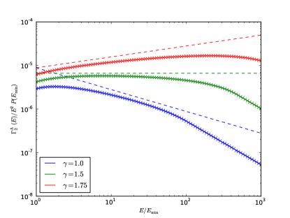
Figure 11.— Energy relaxation as function of energy, for a cusp ($N(>E)\propto E^{3-\gamma}$) with $N_{tot}=10^{4}$ stars and $Q=10^{6}$, for different power-law slopes. The solid lines are the relaxation rates calculated by Eq. (D2), the crosses are the rates calculated using the Cohn & Kulsrud (1978) integrals, the dashed lines are the rates for infinite cusps.

References

- Alexander (1999) Alexander, T. 1999, ApJ, 527, 835
- Alexander (2007) —. 2007, ArXiv e-prints 0708.0688
- Alexander & Hopman (2009) Alexander, T. & Hopman, C. 2009, ApJ, 697, 1861
- Amaro-Seoane et al. (2007) Amaro-Seoane, P., Gair, J. R., Freitag, M., Miller, M. C., Mandel, I., Cutler, C. J., & Babak, S. 2007, Classical and Quantum Gravity, 24, R113
- Amaro-Seoane & Preto (2010) Amaro-Seoane, P. & Preto, M. 2010
- Bahcall & Wolf (1976) Bahcall, J. N. & Wolf, R. A. 1976, ApJ, 209, 214
- Bahcall & Wolf (1977) —. 1977, ApJ, 216, 883
- Bartko et al. (2010) Bartko, H., et al 2010, ApJ, 708, 834
- Bartko et al. (2009) Bartko, H., et al 2009, New Astronomy Reviews, 53, 301
- Binney & Tremaine (2008) Binney, J. & Tremaine, S. 2008, Galactic Dynamics: Second Edition
- Buchholz et al. (2009) Buchholz, R. M., Schödel, R., & Eckart, A. 2009, A&A, 499, 483
- Chandrasekhar (1942) Chandrasekhar, S. 1942, Science, 96, 160
- Chandrasekhar (1943) —. 1943, Reviews of Modern Physics, 15, 1
- Cohn & Kulsrud (1978) Cohn, H. & Kulsrud, R. M. 1978, ApJ, 226, 1087
- Do et al. (2009) Do, T., Ghez, A. M., Morris, M. R., Lu, J. R., Matthews, K., Yelda, S., & Larkin, J. 2009, ApJ, 703, 1323
- Eilon et al. (2009) Eilon, E., Kupi, G., & Alexander, T. 2009, ApJ, 698, 641
- Eisenhauer et al. (2005) Eisenhauer, F., et al 2005, ApJ, 628, 246
- Ferrarese & Merritt (2000) Ferrarese, L. & Merritt, D. 2000, ApJ, 539, L9
- Freitag (2008) Freitag, M. 2008, in Lecture Notes in Physics, Vol. 760, The Cambridge N-Body Lectures, ed. S. J. Aarseth, C. A. Tout, & R. A. Mardling (Dordrecht: Springer Netherlands), 97–121
- Gardiner (2004) Gardiner, C. 2004, Handbook of Stochastic Methods: for Physics, Chemistry and the Natural Sciences (Springer Series in Synergetics) (Springer), 415
- Gebhardt et al. (2000) Gebhardt, K., et al 2000, ApJ, 539, L13
- Ghez et al. (2005) Ghez, A. M., Salim, S., Hornstein, S. D., Tanner, A., Lu, J. R., Morris, M., Becklin, E. E., & Duchene, G. 2005, ApJ, 620, 744
- Ghez et al. (2008) Ghez, et al, 2008, ApJ, 689, 1044
- Gillessen et al. (2009a) Gillessen, S., Eisenhauer, F., Fritz, T. K., Bartko, H., Dodds-Eden, K., Pfuhl, O., Ott, T., & Genzel, R. 2009a, ApJ, 707, L114
- Gillessen et al. (2009b) Gillessen, S., Eisenhauer, F., Trippe, S., Alexander, T., Genzel, R., Martins, F., & Ott, T. 2009b, ApJ, 692, 1075
- Goodman (1983) Goodman, J. 1983, ApJ, 270, 700
- Goodman (1985) —. 1985, In: Dynamics of star clusters; Proceedings of the Symposium, 179
- Hénon (1960) Hénon, M. 1960, Annales d’Astrophysique, 23
- Hopman & Alexander (2006) Hopman, C. & Alexander, T. 2006, ApJ, 645, 1152
- Keshet et al. (2009) Keshet, U., Hopman, C., & Alexander, T. 2009, ApJ, 698, L64
- Khalisi & Spurzem (2006) Khalisi, E. & Spurzem, R. 2006, NBODY6++ Features of the computer - code, ftp://ftp.ari.uni-heidelberg.de/pub/staff/spurzem/nb6mpi/nb6++manual-new.pdf
- Lightman & Shapiro (1977) Lightman, A. & Shapiro, S. 1977, ApJ, 211, 244
- Lin & Tremaine (1980) Lin, D. N. C. & Tremaine, S. 1980, ApJ, 242, 789
- Madigan et al. (2011) Madigan, A.-M., Hopman, C., & Levin, Y. 2011, ApJ, 738, 99
- Merritt (2010) Merritt, D. 2010, ApJ, 718, 739
- Metzler & Klafter (2000) Metzler, R. & Klafter, J. 2000, Physics Reports, 339, 1
- Nelson & Tremaine (1999) Nelson, R. W. & Tremaine, S. 1999, MNRAS, 306, 1
- Peebles (1972) Peebles, P. J. E. 1972, ApJ, 178, 371
- Preto & Amaro-Seoane (2010) Preto, M. & Amaro-Seoane, P. 2010, ApJ, 708, L42
- Preto et al. (2004) Preto, M., Merritt, D., & Spurzem, R. 2004, ApJ, 613
- Rauch & Tremaine (1996) Rauch, K. P. & Tremaine, S. 1996, New Astronomy, 1, 149
- Rosenbluth et al. (1957) Rosenbluth, M. N., MacDonald, W. M., & Judd, D. L. 1957, Physical Review, 107, 1
- Shapiro & Marchant (1978) Shapiro, S. L. & Marchant, A. B. 1978, ApJ, 225, 603
- Spitzer (1987) Spitzer, L. 1987, Princeton
- Spurzem et al. (2001) Spurzem, R., Baumgardt, H., & Ibold, N. 2001, A parallel implementation of an N-body integrator on general and special-purpose computers, ftp.ari.uni-heidelberg.de/pub/staff/spurzem/edinpaper.ps.gz
- Tremaine et al. (2002) Tremaine, S., et al 2002, ApJ, 574, 740
- Weinberg (2001) Weinberg, M. D. 2001, MNRAS, 328, 311
- Weinberg et al. (2005) Weinberg, N. N., Milosavljević, M., & Ghez, A. M. 2005, ApJ, 622, 878
- Yusef-Zadeh et al. (2012) Yusef-Zadeh, F., Bushouse, H., & Wardle, M. 2012, ApJ, 744, 24
- Zumofen & Klafter (1994) Zumofen, G. & Klafter, J. 1994, Chemical physics letters, 2614