]
Relativistic Spin Operator and Lorentz Transformation of the Spin State of a Massive Dirac Particle
We have shown that the covariant relativistic spin operator is equivalent to the spin operator commuting with the free Dirac Hamiltonian. This implies that the covariant relativistic spin operator is a good quantum observable. The covariant relativistic spin operator has a pure quantum contribution that does not exist in the classical covariant spin operator. Based on this equivalence, reduced spin states can be clearly defined. We have shown that depending on the relative motion of an observer, the change in the entropy of a reduced spin density matrix sweeps through the whole range.
pacs:
03.67.-a, 03.30.+pI Introduction
The spin of a massive Dirac particle is , so it can be used as a qubit under the condition that a detector is ideal in the sense that it does not respond to the momentum of the particle. The statistical prediction of measurements for a spin is provided by the reduced spin density matrix, which can be obtained by partial tracing over momentum degrees of freedom. The interesting fact is that the purity of the spin, which is described by the Von Neumann entropy of the reduced spin density matrix, changes under the Lorentz transformation Peres . This would be expected because the spin of a massive Dirac particle rotates depending on the momentum of the particle under the general Lorentz transformation as Wigner has noted Wigner . By the Wigner rotation, the entanglement of spin and momentum degrees of freedom can be changed in general.
The seminal work by Peres et al. Peres , which noticed the relativistic depurification of the spin by using two-component spinors, has not been fully appreciated. There were arguments whether the reduced spin density matrix in Ref. 1 is a proper one Peres1 . This is partly because the physical spin observable was not noted in that paper Peres . The change of the spin entropy can be described by the reduced spin density matrix which does not require the explicit form of a spin observable. For the measurement of the spin entropy, however, the physical spin observables must be specified. Because of the lack of knowledge about the relativistic spin, most later works, which have developed the new field known as the relativistic quantum information Czachor ; Alsing ; Ahn ; Czachor1 ; Peres2 ; Terashima ; Lee ; Kim ; Caban1 ; Caban2 ; Friis ; Gingrich ; Vedral ; Choi , have been done by using spins different from the one implicitly given in the paper Peres .
Gingrich and Adami have used the 4-dimensional Dirac eigen-spinors, which are the spin part of the solution for the covariant Dirac equation, because the eigen-spinors show manifest Lorentz covariance Gingrich . The Dirac eigen-spinor in a laboratory frame, where a particle is moving, has momentum-dependent components, so partial tracing over the momentum was criticized Czachor1 . The momentum dependence in the components of the Dirac eigen-spinors can be eliminated in the special representation given by Foldy and Woutheysen Foldy . We call this the Foldy-Woutheysen (FW) representation. Therefore, in the FW representation, the meaning of partial tracing over the momentum is clear so that the reduced spin density matrix can be well defined. The two spin density matrices for the same positive energy particle, one in the FW representation and the other in the covariant Dirac representation, give the same entropy. In this sense the results given by Peres et. al Peres and Gingrich and Adami Gingrich can be justified. Recently it was noticed, however, that the reduced spin density matrix was meaningless because the spin of the relativistic particle could not be measured independently of its momentum Vedral . This conclusion is erroneous because the classical spin operator, not the full quantum spin operator, had been considered ChoiNote .
In the FW representation, there is a mean spin operator that commutes with the free Dirac Hamiltonian so that
it is a good quantum observable.
We call this spin operator the FW mean spin operator. Grsey and Ryder Gursey have shown that the covariant
relativistic spin operator for positive energy states,
which is obtained by using the Lorentz transformation in the spinor representation, is
the same as a FW mean spin operator for positive energy states.
The equivalence for negative energy states, however, is not clear because the forms of two operators are different.
In this paper, we will show explicitly the equivalence between the covariant relativistic spin operator and
the FW mean spin operator for the whole of spinor space.
The difference of the covariant relativistic spin operator from the classical covariant spin operator will also be discussed.
This will clarify the long-standing controversy regarding what are the proper spin operator
and the reduced spin entropy in the laboratory frame.
We will also study the change of the relativistic spin entropy
in the FW representation in which the tracing over the momentum has a clear meaning.
The results show that the pure spin state can become a completely-mixed spin state and vice versa.
In Sections II and III, we review the covariant relativistic spin operator and
the FW mean spin for clarity and self-containedness.
In Section IV, we will show the equivalence of the two spin operators.
In Section V, we will discuss the change of reduced spin density matrices
under Lorentz transformation.
In Section VI, we will summarize our results.
II covariant relativistic spin
The spin operator in the laboratory frame can be obtained from the spin operator
in the particle rest frame by using the Lorentz transformation .
This spin operator is a good candidate for a relativistic spin operator, and
we call this spin operator the covariant relativistic spin operator.
We will review the procedure to obtain the covariant relativistic spin in a fully covariant way and discuss
its difference from the classical covariant spin used to define the covariant spin magnetic dipole
moment. For completeness, we also review another approach Ryder99 to obtain the covariant relativistic spin
operator by using Pauli-Lubanski vector.
II.1 Lorentz Covariant Approach
Let us consider the following covariant Dirac equation for a free massive Dirac particle in coordinate space:
| (1) |
where
| (6) |
and are the usual Pauli matrices. are Dirac matrices. We use the sign convention for the metric and the natural units . The summation conventions are also used. The Greek index runs and the Latin index runs . The covariant Dirac equation has two positive energy solutions, , and two negative energy solutions, , where . is the coordinate representation of the momentum eigenstate. and are the spin parts of the Dirac solutions and are called the positive energy spinor and the negative energy spinor, respectively. As is well known, negative energy solutions can be interpreted as antiparticles with opposite charges from and the same momenta as those of the particles even when their momentum eigenvalue is Ryder1 . In this paper, we will use the term negative energy spinor because its use is convenient for a one-particle state.
Using the Lorentz covariance of the Dirac equation in Eq. (1), one can obtain the solutions for a moving particle from the solutions in the particle rest frame by using the Lorentz transformation. The momentum of particle is determined from the momentum of the rest particle such as by using the standard Lorentz boost . Then, the spinors and for moving particles can be obtained by the spinors and for the rest particle multiplying by , respectively. That is, and . The is the Lorentz transformation in the spinor representation corresponding to :
| (9) |
where is the rapidity of the particle and . In the particle rest frame, the meaning of the spin index is clear because the spin operator in the particle rest frame is
| (12) |
where and are the three-dimensional vectors and , respectively. The spinors and are eigen-spinors of the 4-dimensional Pauli spin matrix with eigenvalue .
Note that the spinors and for moving particles have the same spin index as the rest spinors and . This is reasonable because Wigner rotation by a single standard Lorentz transformation becomes trivial Wigner . However, the spin operator in the laboratory frame is not clear. The spin operator in Eq. (12) is in the particle rest frame, and is the space part of the Pauli-Lubanski vector
| (13) |
where and are the angular momentum and the momentum operators, respectively. is a Levi-Civita symbol. The in the laboratory frame, however, does not satisfy the required spin commutation relations although is the second Casimir invariant of the inhomogeneous Lorentz group (Poincar group) and is the spin of the particle Ryder1 .
The proper way to obtain the relativistic spin operator in a fully covariant way is to define the following spin tensor for the particle rest frame:
| (14) |
In the standard representation, the 3-dimensional spin vector defined by becomes the Pauli spin , where is a Levi-Civita symbol. The spin operator for a moving frame can naturally be defined, by using the Lorentz transformation, from the spin tensor for the particle rest frame as
| (15) |
where is the inverse Lorentz transformation of . Then the spin operator becomes
| (16) |
which is the same as the covariant relativistic spin operator in Ref. 20. The is a matrix with off-diagonal terms. Notice that the eigenvalue equations of the covariant relativistic spin operator in the laboratory frame are
| (17) | |||||
These confirm that the spin eigenvalues in the laboratory frame are the same as the spin eigenvalues in the particle rest frame. An arbitrary positive energy spin state in the particle rest frame becomes the spin state in the moving frame. Then, the expectation value of the spin in the particle rest frame is equal to the expectation value of the spin in the moving frame , where and the relativistic invariant normalizations
| (18) |
are used. This implies that the measurements of the spin along the same axes by two observers, one in the particle rest frame and the other in the laboratory frame, will give the same spin expectation value.
It is interesting to compare the covariant relativistic spin operator in Eq. (16) with the classical covariant spin in classical electrodynamics. The classical covariant spin can be defined as by using the classical covariant magnetic dipole moment Penfield
| (19) |
where is the gyromagnetic ratio. The Lorentz factor is and
.
Notice that the classical covariant spin can also be derived by using the spin tensor
.
One can see the main difference between the covariant relativistic spin
operator and the classical spin operator
is the proportional term.
That is, without the proportional term, the covariant relativistic spin operator
becomes ,
where is the identity matrix.
Therefore, the proportional term is a purely quantum-mechanical term that is manifest
in the 4-dimensional spinor representation.
II.2 Construction by Using Commutators of Pauli-Lubanski Vectors
The Dirac particles satisfy the inhomogeneous Lorentz group (Poincar group) symmetry. There are two Casimir operators in the Poincar group, the first Casimir invariant and the second Casimir invariant . Thus, it was expected that the covariant relativistic spin operator could be constructed directly by using the Pauli-Lubanski vector. The covariant relativistic spin operator, however, cannot be obtained by using simple linear combinations of the components of the Pauli-Lubanski vector. The only candidate for the component of the angular momentum vector that is a linear function of was shown to be Bogolubov
| (20) |
In fact the above equation is the spin operator in the particle rest frame which is written in the laboratory frame by using .
Ryder has given the correct way to construct the spin operator, different from the usual Pauli spin operator , by using the Pauli-Lubanski vector Ryder99 . First, the following two antisymmetric tensor operators are defined by using the commutators of the Pauli-Lubanski vectors:
| (21) |
Then, the two tensor operators,
| (22) |
satisfy the commutation relations for the angular momentum. Therefore, these two tensor operators can be represented by matrices which cannot be irreducible representations under the parity. The 4-dimensional irreducible spin tensor including parity can be constructed as
| (23) |
Then, the spatial component defined by
becomes the same as the covariant relativistic spin operator in Eq. (16).
III Canonical approach
In this section, we will review the canonical approach given by Foldy and Woutheysen Foldy . The covariant relativistic spin operator was obtained in the last section; however, it is not clear whether the covariant relativistic spin operator is a good quantum observable in the sense that good quantum observables must commute with the Hamiltonian of a particle. In the canonical approach, the following free Dirac Hamiltonian is used to describe a massive Dirac particle in the laboratory frame:
| (24) |
The is a momentum operator such that the eigenvalues for a positive energy state and a negative energy state are , respectively. In the particle rest frame, the covariant relativistic spin operator and the free Dirac Hamiltonian commute with each other. In the laboratory frame, however, the covariant relativistic spin operator does not commute with the free Dirac Hamiltonian in Eq. (24) because the Dirac Hamiltonian in the laboratory frame cannot be obtained simply, by using the Lorentz transformation, from the Dirac Hamiltonian in the particle rest frame as a covariant relativistic spin operator.
Foldy and Woutheysen (FW) found the mean spin operator that commutes with the Dirac Hamiltonian for a moving particle by using the following canonical transformation Foldy :
| (25) |
In the new representation, the Dirac Hamiltonian has a diagonal form such as , where represents the operator that gives eigenvalues . We call this new representation the FW representation. In the FW representation, a spinor transforms as
| (26) |
where are the positive energy and the negative energy Dirac spinors in the standard representation such that . We use the symbol for objects in the FW representation. Here, the factor is required because of the different normalizations in the canonical representation and in the covariant representation. In the canonical representation, normalizations are used, but normalizations are used in the covariant representation.
Notice that the Dirac Hamiltonian of the moving particle in the FW representation has the diagonal form . Therefore, the Pauli spin operator commutes with the transformed Hamiltonian ; hence, the spin operator becomes a good spin observable in the FW representation. The spin operator for a moving particle in the FW representation, which is , has the following positive and negative energy eigen-spinors:
| (27) | |||
where the superscript T means the transpose of a vector.
The spin operator in the FW representation is transformed to the FW mean spin operator in the standard representation as
| (28) |
One can easily check that the FW spin operator commutes with
the Dirac Hamiltonian by direct calculation.
This means the FW mean spin operator is a constant of motion and
becomes a good quantum observable in the standard representation.
As mentioned in Ref. 18, the spin operator is nonlocal
because it depends on the momentum.
In fact, the eigenvalue of the FW mean spin operator represents the average spin of a rapidly oscillating particle within its
Compton wavelength. This is the meaning of the name ’FW mean spin operator.’
The FW mean spin operator has been shown to be the spin operator in the non-relativistic Pauli Hamiltonian Foldy .
This implies that the expectation value measured by experiments in non-relativistic quantum mechanics
is the expectation value of this spin operator.
IV Equivalence between relativistic spin and FW mean spin
The covariant relativistic spin has been shown by several authors to be equivalent to the Foldy-Woutheysen spin for the positive energy states Gursey . For the positive energy spinors, the spinor representation of the standard Lorentz transformation in Eq. (9) can be represented by the unitary operator in Eq. (25) with the normalization factor , so the equivalence of the two spin operators can be given at the operator level. The spinor representation of the Lorentz transformation acting on the entire spinor space, however, cannot be a unitary operator because the Lorentz group has no finite dimensional unitary representation. At this stage, therefore, it is unclear that the covariant relativistic spin operator is equivalent to the FW mean spin operator for negative energy states. In fact, the two spin operators, the covariant relativistic spin in Eq. (16) and the FW mean spin in Eq. (28), are different. This raises a question as to which spin operator is the proper spin observable for a massive Dirac particle. We will show that they are equivalent in the sense that they give the same expectation values.
The equivalence of the two spin operators can be obtained by using the relations between the actions of the Lorentz transformation and the unitary transformation on positive and negative energy spinors. The unitary operator has the momentum operator , which gives different eigenvalues for positive energy and negative energy spinors. Thus, it is convenient to use the projection operators such that
| (29) | |||||
| (30) |
One can define and , which satisfy , and . That is, and project out positive and negative energy spinors, respectively. Then, the following relations hold:
| (31) | |||||
Using these relations, we obtain the equivalences
| (32) |
and
| (33) |
because and . The sign and are due to the relativistic invariant normalization in Eq. (18).
Equations (32) and (33) guarantee that the expectation values of
the FW mean spin operator and the covariant relativistic spin operator are the same for the general spinor
, which is a linear combination of the positive and the negative eigen-spinors.
In this sense, the two spin operators are equivalent. As a result,
the covariant relativistic spin operator can be considered as a good quantum observable
because it is equivalent to the FW mean spin operator that commutes with the free Dirac Hamiltonian.
V Reduced Spin Density Operator
For the study of a reduced spin density operator, the momentum representation of the covariant Dirac equation is convenient. The solutions of the covariant Dirac equation in the momentum representation can be represented as for positive energy solutions and for negative energy solutions. is the momentum eigenstate; i.e., . The spin expectation value of a spinor in the laboratory frame has been shown to be the same as the spin expectation value of the spinor in the particle rest frame. This implies that a reduced spin density matrix can be clearly defined by a partial tracing over momentum degrees of freedom. To make this point more transparent, we will study the reduced spin density matrices in the FW representation because the spin and the momentum degrees of freedoms are decoupled in the FW representation as are those in the particle’s rest frame. In the FW representation, the meaning of the partial trace over the momentum is clear.
We consider the following state in the FW representation:
| (34) |
The normalization requires . For the density matrix , the reduced spin density matrix is well defined by a partial trace over momentum as
The reduced spin density matrix becomes the same as the non-relativistic spin density matrix for a positive energy particle.
The relativistic effects on the reduced spin density matrix of a moving particle is represented by the transformation of the reduced spin density matrix under a general Lorentz transformation The transformation of the reduced spin density matrix is given by the transformation matrix of the spinor under the Lorentz transformation. We have obtained the transformation matrix for the positive energy spinors in a previous work Choi . In this section, the complete transformation matrix for the whole of spinor space is obtained. The complete transformation matrix in the FW representation will be shown to be equivalent to the complete transformation matrix in the covariant representation.
Let us assume that the two observers and are related by an arbitrary Lorentz transformation . Lorentz transformations do not change the sign of the energy for a free particle, so we must deal with the positive and the negative energy states separately. The transformation matrix in the covariant representation and the transformation matrix in the FW representation for the positive energy spinors have the following relations:
where is the space part of the four momentum . This equation shows that the transformation matrix in the covariant representation is equivalent to the transformation matrix in the FW representation because the forms of and are the same. The transformation matrices for the negative energy spinor is obtained in a similar manner. As a result, the complete transformation matrix can effectively be written in the following block diagonal form:
| (41) |
where and . This transformation matrix shows that the irreducible representation for the Lorentz transformation is the unitary matrix . This two-dimensional matrix corresponds to the two-dimensional unitary representation of the Wigner rotation. This means the FW representation and the covariant representation are two equivalent representations for Wigner’s little group.
Now, we will consider the change in the reduced spin density matrix under the Lorentz transformation . The transformation of the spinor is obtained as
| (42) |
The reduced spin density matrix for the observer , defined by
| (43) |
shows the dependence of the rotation of the spin not only on the Lorentz transformation but also on the momentum of the particle. This momentum-dependent rotation changes the entanglement between the spin and the momentum degrees of freedom. As a result, the spin entropy, which describes the mixedness of the reduced spin density matrix, changes.
The reduced spin density matrix for the general state in Eq. (34) is too complicated to study the essential feature of the spin density matrix under the general Lorentz transformation. Therefore, we will consider a simple example that shows the nontrivial effects under the Lorentz transformation. We consider the following two initial positive energy states in the FW representation:
| (44) | |||||
| (45) |
where the four momentum and . is included due to the normalization . The space parts of the momentum are written in spherical coordinate as and . is perpendicular to and corresponds to the replacement of by . is the polar angle from the positive -axis, and is the azimuthal angle in the plane from the -axis. The action of a rotation of an observer is trivial because the rotation does not change the entanglement between the momentum degrees of freedom and the spin degrees of freedom. Therefore, we consider the Lorentz boost in the direction with rapidity . This does not reduce the generality because the general momentum vector is considered. The reduced spin density matrices can be described by matrices because the positive energy spinors in the FW representation can be represented by two-component vectors. The reduced spin density matrices and are obtained by tracing over the momentum for the density matrices and , respectively. The becomes the pure state , and the becomes the complete mixed state . Note that the two-dimensional representations of the spinors in the FW representation are described by , which are the eigenstates of the usual Pauli matrix with eigenvalues such that .
The transformed spin density matrices become
| (46) | |||||
| (49) |
and
| (50) | |||||
| (53) |
The parameters , , and are
| (54) | |||||
| (55) | |||||
| (56) |
where and .
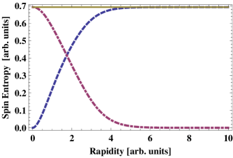
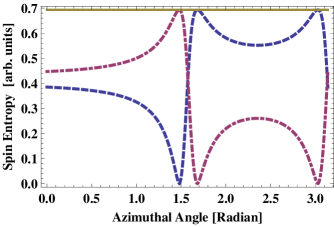
We will study the change in the purification of the spin by using the entropy of the spin density matrix. The entropy for the state is defined as Peres3
| (57) |
where is an eigenvalue of . The spin density matrices transform nontrivially under a Lorentz transformation as shown in Eq. (46) and Eq. (50), so the spin entropies will also change nontrivially. The results are shown in Fig. 1 and Fig. 2. For explicit calculations, we have set the momentum and the rest mass . Fig 1 shows the dependence on the rapidity for . The magnitude of the observer’s velocity becomes for . The changes of spin entropies with increasing rapidity in this figure show that the pure state can be changed to the completely mixed state and vice versa. Fig 2 shows the polar angle dependence of the spin entropies for the rapidity . The spin entropies in this figure show that depending on the polar angle, the Lorentz transformation changes the mixedness of the spin over the whole range.
Because the transformation matrices and
in the covariant representation and in the FW representation
are equivalent, the behaviors of the reduced spin density matrix in the two representations are the same.
The difference in the two representations are the normalizations. In the covariant representation,
the density matrix for the observer is defined as
to guarantee the Lorentz invariance of the normalization.
The trace over momentum is also represented by the Lorentz invariant measure .
VI Summary
In summary, we have shown the equivalence between the covariant relativistic spin and the FW mean spin of a Dirac particle. Based on the equivalence, the covariant relativistic spin operator is clearly a good spin operator in the covariant representation. As a result, the spin index of the Dirac spinor can be understood to represent the spin eigenvalues of the moving particle. The covariant relativistic spin is shown to have a pure quantum contribution, which cannot be given by the classical spin. In the FW representation, the Dirac Hamiltonian for a moving particle assumes a diagonal form of the Hamiltonian in the particle rest frame. This fact makes dealing with the momentum and the spin degrees of freedom separately easy.
We have studied the relativistic effects on the spin state in the FW representation.
The spin state can be defined by tracing over the momentum degrees of freedom for the complete density matrix.
The trace over the momentum is obtained by integrating over the momentum, which was considered ambiguous
in the Dirac spinor because of momentum-dependent components.
This ambiguity can be cleared by considering the problem in the FW representation, which has been shown to be
equivalent to the covariant representation.
The spin entropy, which describes the purity of the spin, changes under the Lorentz transformation.
The pure spin state can become a totally mixed spin state and vice versa under the Lorentz transformation.
Therefore, the entropy of the spin is neither a Lorentz invariant nor covariant.
ACKNOWLEDGMENTS
The authors are grateful for helpful discussions with Prof. Jaewan Kim at Korea Institute for Advanced Study. This work was supported by a National Research Foundation of Korea grant funded by the Korean Government (2011-0005740).
References
- (1) A. Peres, P. F. Scudo, and D. R. Terno, Phys. Rev. Lett. 88, 230402 (2002).
- (2) E. Wigner, Ann. Math. 40, 149 (1939).
- (3) M. Czachor, Phys. Rev. Lett. 94, 078901 (2005); A. Peres, P. F. Scudo, and D. R. Terno, Phys. Rev. Lett. 94, 078902 (2005).
- (4) M. Czachor, Phys. Rev. A 55, 72 (1997); Phys. Rev. Lett. 94, 078901 (2005).
- (5) P. M. Alsing and G. J. Milburn, Quant. Inf. Comput. 2, 487 (2002); Phys. Rev. Lett. 91, 180404 (2003).
- (6) D. Ahn, H. J. Lee, Y. H. Moon, and S. W. Hwang, Phys. Rev. A 67, 012103 (2003).
- (7) M. Czachor and M. Wilczewski, Phys. Rev. A 68, 010302(R) (2003).
- (8) H. Terashima and M. Ueda, Quantum Inf. Comput. 3, 224 (2003).
- (9) A. Peres and D. R. Terno, Rev. Mod. Phys. 76, 93 (2004), and references therein.
- (10) D. Lee and C-Y. Ee, New J. Phys. 6, 67 (2004).
- (11) W. T. Kim and E. J. Son, Phys. Rev. A 71, 014102 (2006).
- (12) P. Caban and J. Rembieliński, Phys. Rev. A 72, 012103 (2005); ibid 74, 042103 (2006).
- (13) P. Caban, A. Dziegielewska, A. Karmazyn and M. Okrasa, Phys. Rev. A 81, 032112 (2010).
- (14) N. Friis, R. A. Bertlmann, M. Huber and B. C. Hiesmayr, Phys. Rev. A 81, 042114 (2010).
- (15) R. M. Gingrich and C. Adami, Phys. Rev. Lett. 89, 270402 (2002).
- (16) P. L. Saldanha and V. Vedral, New J. Phys. 14, 023041 (2012); Phys. Rev. A 85, 062101 (2012).
- (17) T. Choi, J. Hur and J. Kim, Phys. Rev. A 84, 012334 (2011).
- (18) L. L. Foldy and S. A. Woutheysen, Phys. Rev. 78, 29 (1950).
- (19) Note that the classical magnetic dipole moment in Eq. (11) is the same as the magnetic dipole moment in Eq. (6) of Ref. 16.
- (20) F. Grsey, Phys. Lett. 14, 330 (1965); L. H. Ryder, J. Phys. A: Math. Gen. 31, 2465 (1998).
- (21) L. H. Ryder, Gen. Rel. Grav. 31, 775 (1999).
- (22) L. H. Ryder, Quantum Field Theory (Cambridge University Press, Cambridge, U.K., 1996).
- (23) P. Penfield and H. A. Haus Electrodynamics of Moving Media (MIT Press, Cambridge, MA, 1967).
- (24) N. N. Bogolubov, A. A. Logunov, and I. T. Torov, Introduction to Axiomatic Quantum Field Theory (Benjamin, Reading, MA, 1975).
- (25) A. Peres, Quantum Theory: Concepts and Methods (Kluwer Academic Publishers, Dordrecht, 1995).